Lecture 4Conduct of Monetary Policy: Goals, Instruments, and Targets;

Time Inconsistency and Targeting Rules

1. Introduction

In this chapter, we analyze the conduct of monetary policy (or the operating pro-

cedure) i.e. how is it operationalized, what is its objectives, constraints faced by central

banks etc. Central banks are normally mandated to achieve certain goals such as price sta-

bility, high growth, low unemployment etc. But central banks do not directly control these

variables. Rather they have set of instruments such as open-market operations, setting

bank rate etc. which they can use to achieve these objectives.

The problem of central bank is compounded by the fact that their instruments do not

directly affect these goals. These instruments affect variables such as money supply and

interest rates, which then affect goal variables with lag. In addition, these lags may be

uncertain. Due to above mentioned problems, in the conduct of monetary policy distinction

is made among (i) goals (or objectives), (ii) targets (or intermediate targets), (iii) indicators

(or operational targets), and (iv) instruments (or tools).

Target and indicator variables lie between goal and instrument variables. Target

variables such as money supply and interest rates have direct and predictable impact on

goal variables and can be quickly and more easily observed. In previous chapters, we

studied various theories linking target variables to goal variables. By observing these

variables, the central bank can determine whether its policies are having desired effect

or not. However, even these target variables are not directly affected by central bank

instruments. These instruments affect target variables, through another set of variables

called indicators. These indicators such as monetary base and short run interest rates

are more responsive to instruments. The conduct of monetary policy can be represented

schematically as follows:

Instruments → Indicators → Targets → Goals

Following is the list of different kinds of variables.

1

Table 1

Goals or Objectives

1. High Employment

2. Economic Growth

3. Price Stability

4. Interest-Rate Stability

5. Stability of Financial Markets

6. Stability in Foreign Exchange Markets

Targets or Intermediate Targets

1. Monetary Aggregates (M1, M2, M3 etc.)

2. Short Run and Long Run Interest Rates

Indicators or Operational Targets

1. Monetary Base or High-Powered Money

2. Short Run Interest Rate (Rate on Treasury Bill, Overnight Rate)

Instruments or Tools

1. Open Market Operations

2. Reserve Requirements

3. Operating Band for Overnight Rate

4. Bank Rate

Though we have listed six goals, it does not mean that different countries and regimes

give same weight to all these goals. Different goals may get different emphasis in different

countries and times. Currently in Canada, a lot of emphasis is put on the goal of price

and financial market stability. Also, all the goals may not be compatible with each other.

For instance, goal of price stability may conflict with the goals of high employment and

stability of interest rate at least in the short run.

2

The list of target variables raises the question: how do we choose target variables?

Three criteria are suggested: (i) measurability, (ii) controllability, and (iii) predictable

effects on goals.

Quick and accurate measurement of target variables are necessary because the target

will be useful only if it signals rapidly when policy is off track. For a target variable to

be useful, a central bank must be able to exercise effective control over it. If the central

bank cannot exercise effective control over it, knowing that it is off-track is of little help.

Finally and most importantly, target variables must have a predictable impact on goal

variables. If target variables do not have predictable impact on goal variables, the central

bank cannot achieve its goal by using target variables. Monetary aggregates and short and

long run interest rates satisfy all three criteria.

The same three criteria are used to choose indicators. They must be measurable, the

central bank should have effective control over them, and they must have predictable effect

on target variables. All the indicators listed above satisfy these criteria.

2. Money Supply Process, Asset Pricing, and Interest Rates

In previous chapters, we extensively analyzed relationships among goal variables such

employment, inflation, output and target variables such as money supply and interest

rates. Now we turn to analyze relationship among instruments, indicators, and targets.

In order to understand relationships among these three types of variables, it is instructive

to analyze the money supply process and asset pricing which throws light on relationships

among different types of interest rates.

A. Money Supply Process

So far, we have been vague about what determines money supply. We just assumed

that it is partly determined by the central bank and partly by non-policy shocks. In this

section, we take a closer look at the money supply process. It has important bearing on

the conduct of monetary policy.

There are four important actors, whose actions determine the money supply – (i)

the central bank, (ii) banks, (iii) depositors, and (iv) borrowers. Of the four players, the

3

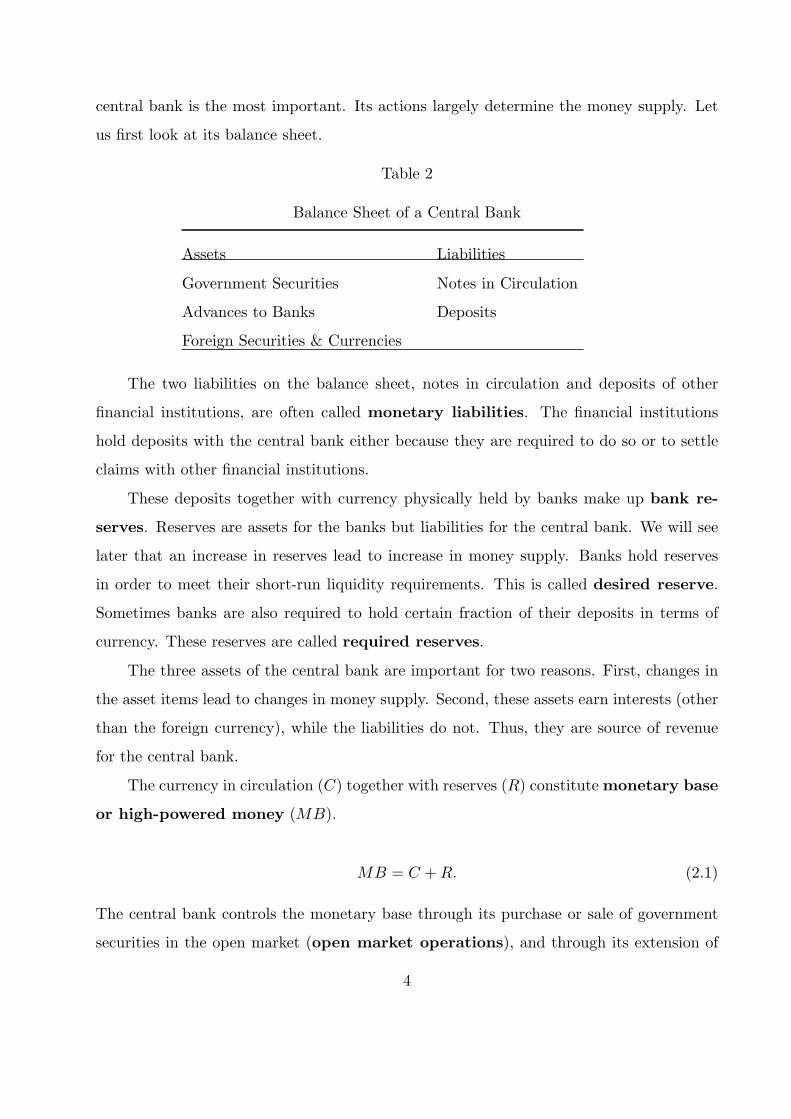
central bank is the most important. Its actions largely determine the money supply. Let

us first look at its balance sheet.

Table 2

Balance Sheet of a Central Bank

Assets Liabilities

Government Securities Notes in Circulation

Advances to Banks Deposits

Foreign Securities & Currencies

The two liabilities on the balance sheet, notes in circulation and deposits of other

financial institutions, are often called monetary liabilities. The financial institutions

hold deposits with the central bank either because they are required to do so or to settle

claims with other financial institutions.

These deposits together with currency physically held by banks make up bank re-

serves. Reserves are assets for the banks but liabilities for the central bank. We will see

later that an increase in reserves lead to increase in money supply. Banks hold reserves

in order to meet their short-run liquidity requirements. This is called desired reserve.

Sometimes banks are also required to hold certain fraction of their deposits in terms of

currency. These reserves are called required reserves.

The three assets of the central bank are important for two reasons. First, changes in

the asset items lead to changes in money supply. Second, these assets earn interests (other

than the foreign currency), while the liabilities do not. Thus, they are source of revenue

for the central bank.

The currency in circulation (C) together with reserves (R) constitute monetary base

or high-powered money (MB).

MB = C + R. (2.1)

The central bank controls the monetary base through its purchase or sale of government

securities in the open market (open market operations), and through its extension of

4

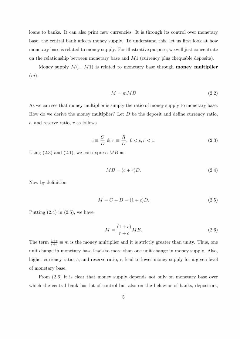
loans to banks. It can also print new currencies. It is through its control over monetary

base, the central bank affects money supply. To understand this, let us first look at how

monetary base is related to money supply. For illustrative purpose, we will just concentrate

on the relationship between monetary base and M1 (currency plus chequable deposits).

Money supply M(≡ M1) is related to monetary base through money multiplier

(m).

M = mMB (2.2)

As we can see that money multiplier is simply the ratio of money supply to monetary base.

How do we derive the money multiplier? Let D be the deposit and define currency ratio,

c, and reserve ratio, r as follows

c ≡ C

D& r ≡ R

D, 0 < c, r < 1. (2.3)

Using (2.3) and (2.1), we can express MB as

MB = (c + r)D. (2.4)

Now by definition

M = C + D = (1 + c)D. (2.5)

Putting (2.4) in (2.5), we have

M =(1 + c)r + c

MB. (2.6)

The term 1+cr+c ≡ m is the money multiplier and it is strictly greater than unity. Thus, one

unit change in monetary base leads to more than one unit change in money supply. Also,

higher currency ratio, c, and reserve ratio, r, lead to lower money supply for a given level

of monetary base.

From (2.6) it is clear that money supply depends not only on monetary base over

which the central bank has lot of control but also on the behavior of banks, depositors,

5

and borrowers which determine currency ratio, c, and reserve ratio, r. c and r depend

on rate of return on other assets and their variability, innovations in financial system and

cash management, expected deposit outflows etc. In general, broader the measure of money

supply, less control the central bank has on its supply.

B. Asset Pricing and Interest Rates

In the analysis so far, we divided financial assets in two categories – monetary and

non-monetary assets. We called the rate of return on non-monetary assets as the nominal

rate of interest. But we know that there are different types of non-monetary assets with

different rates of return. Then the question is : how justifiable is lumping together of

different non-monetary assets?

We can lump together different types of non-monetary assets provided there is stable

relationship among their rates of return. The rate of return on an asset depends on its

pay-off and price. In order to understand, the relationships among rates of return, we need

to know how assets are priced. This analysis helps us in establishing relationship among

different types of interest rates.

The price of an asset equates the marginal cost (in utility terms) to its expected

marginal benefit (in utility terms). Suppose that an asset pays off at time t + i with i ≥ 1

and its payoff is yt+i (suppose resale value is 0), which is a random variable. Then its price

at time t, qt satisfies

qtu′(ct) = βiEt [u′(ct+i)yt+i] . (2.7)

The left hand side is the marginal cost of buying the asset in utility terms and the right

hand is the expected marginal benefit. The asset pays off yt+i in period t + i, which is

converted in utility terms by multiplying it with the marginal utility of consumption at

t + i. To make it comparable to time t utility, we multiply it by βi. (2.7) can be rewritten

as

qt = βiEt

[u′(ct+i)yt+i

u′(ct)

]. (2.8)

6

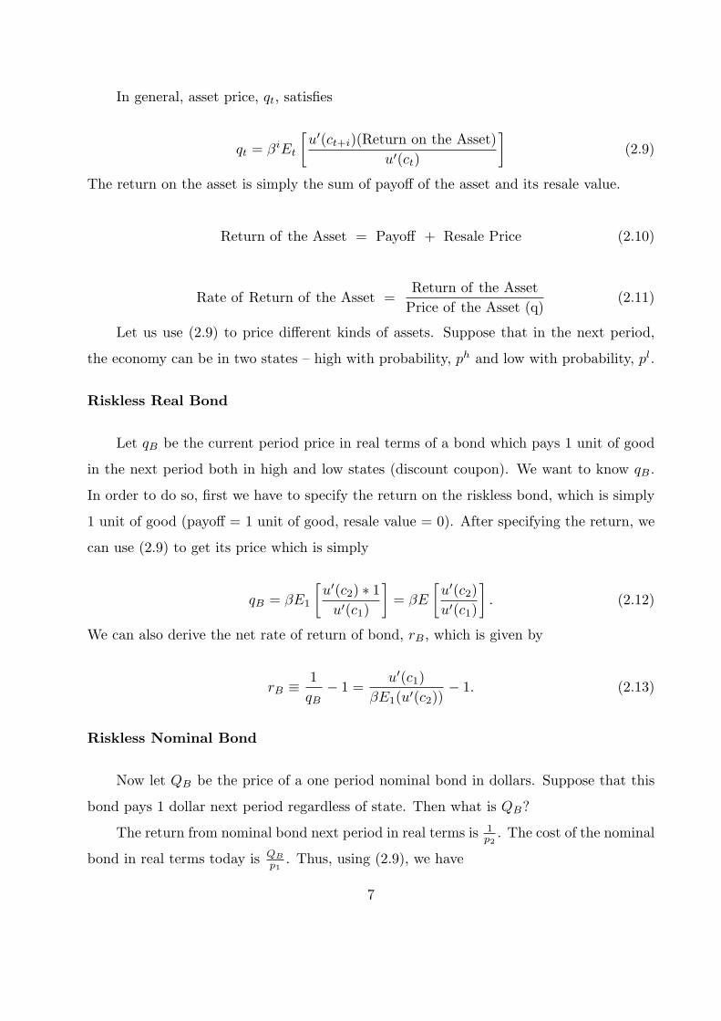
In general, asset price, qt, satisfies

qt = βiEt

[u′(ct+i)(Return on the Asset)

u′(ct)

](2.9)

The return on the asset is simply the sum of payoff of the asset and its resale value.

Return of the Asset = Payoff + Resale Price (2.10)

Rate of Return of the Asset =Return of the Asset

Price of the Asset (q)(2.11)

Let us use (2.9) to price different kinds of assets. Suppose that in the next period,

the economy can be in two states – high with probability, ph and low with probability, pl.

Riskless Real Bond

Let qB be the current period price in real terms of a bond which pays 1 unit of good

in the next period both in high and low states (discount coupon). We want to know qB .

In order to do so, first we have to specify the return on the riskless bond, which is simply

1 unit of good (payoff = 1 unit of good, resale value = 0). After specifying the return, we

can use (2.9) to get its price which is simply

qB = βE1

[u′(c2) ∗ 1

u′(c1)

]= βE

[u′(c2)u′(c1)

]. (2.12)

We can also derive the net rate of return of bond, rB , which is given by

rB ≡ 1qB

− 1 =u′(c1)

βE1(u′(c2))− 1. (2.13)

Riskless Nominal Bond

Now let QB be the price of a one period nominal bond in dollars. Suppose that this

bond pays 1 dollar next period regardless of state. Then what is QB?

The return from nominal bond next period in real terms is 1p2

. The cost of the nominal

bond in real terms today is QB

p1. Thus, using (2.9), we have

7

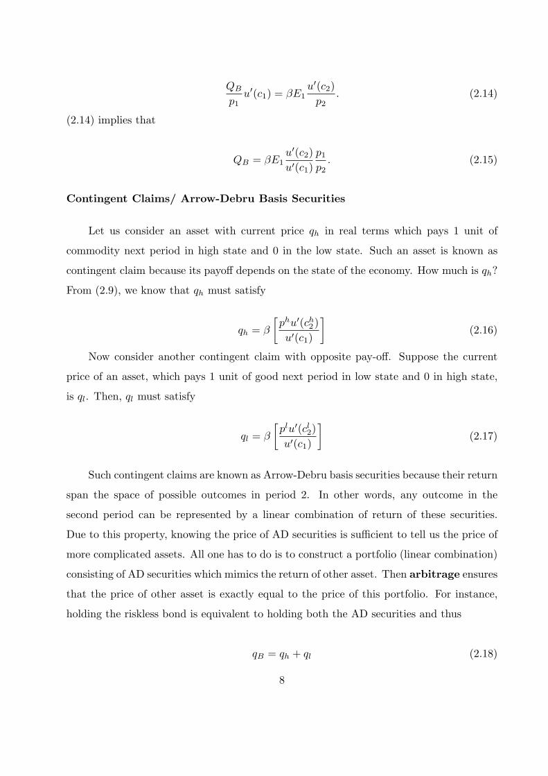
QB

p1u′(c1) = βE1

u′(c2)p2

. (2.14)

(2.14) implies that

QB = βE1u′(c2)u′(c1)

p1

p2. (2.15)

Contingent Claims/ Arrow-Debru Basis Securities

Let us consider an asset with current price qh in real terms which pays 1 unit of

commodity next period in high state and 0 in the low state. Such an asset is known as

contingent claim because its payoff depends on the state of the economy. How much is qh?

From (2.9), we know that qh must satisfy

qh = β

[phu′(ch

2 )u′(c1)

](2.16)

Now consider another contingent claim with opposite pay-off. Suppose the current

price of an asset, which pays 1 unit of good next period in low state and 0 in high state,

is ql. Then, ql must satisfy

ql = β

[plu′(cl

2)u′(c1)

](2.17)

Such contingent claims are known as Arrow-Debru basis securities because their return

span the space of possible outcomes in period 2. In other words, any outcome in the

second period can be represented by a linear combination of return of these securities.

Due to this property, knowing the price of AD securities is sufficient to tell us the price of

more complicated assets. All one has to do is to construct a portfolio (linear combination)

consisting of AD securities which mimics the return of other asset. Then arbitrage ensures

that the price of other asset is exactly equal to the price of this portfolio. For instance,

holding the riskless bond is equivalent to holding both the AD securities and thus

qB = qh + ql (2.18)

8

Long and Short Bonds

Let qL be the price of a bond today, which pays 1 unit in period 3 (long or two-

period bond), and qS1 be the price of one period bond, which pays 1 unit next period. Let

u(c) = ln c. Then,

qL = β2E1

[c1

c3

](2.19)

qS1 = βE1

[c1

c2

](2.20)

From (2.19) and (2.20), we can derive rates of interest on long and short bonds. The gross

return on long bond satisfies

(1 + rL)2 =1qL

=1

β2E1

[c1c3

] . (2.21)

Similarly, the gross return on short bond satisfies

1 + rS1 =

1qS1

=1

βE1

[c1c2

] . (2.22)

The pattern of returns on long and short bonds are known as term structure. The plot

of term structure over maturity is also known as yield curve. The term structure or yield

curve embodies the forecasts of future consumption growth. In general, yield curve slopes

up reflecting growth. Downward sloping yield curve often forecasts a recession.

What is the relationship between the prices of short and long bonds? We turn to

covariance decomposition (E(xy) = E(x)E(y) + cov(x, y)).

qL = β2E1

[c1c2

c2c3

](2.23)

which implies

qL = qS1 E1q

S2 + Cov

(βc1

c2,βc2

c3

)(2.24)

9

where qS2 is the second period price of one period bond. If we ignore the covariance term,

then in terms of returns (2.24) can be written as

(1

1 + rL

)2

=1

1 + rS1

E11

1 + rS2

. (2.25)

Taking logarithms, utilizing the fact that ln(1+r) ≈ r, and ignoring Jensen’s inequal-

ity we get

rL ≈ rS1 + E1r

S2

2. (2.26)

(2.26) suggests that the long run bond yield is approximately equal to the arithmetic mean

of the current and expected short bond yields. This is called expectation hypothesis

of the term structure. (2.24 - 2.27) imply that prices of different types of bonds and thus

their return are related to each other. Thus, if one type of rate of interest changes, its

effect spreads to other interest rates as well.

Exercise: Find out the prices of short and long term nominal bonds and their rela-

tionship.

Exercise: What is the price of bond which pays 1 unit of good in period T in all states?

Forward Prices

Suppose in period 1, you sign a contract, which requires you to pay f in period 2

in exchange for a payoff of 1 in period 3. How do we value this contract? Notice that

the price of contract, which is to be paid in period 2, is agreed in period 1. Then the

expected marginal cost of the contract in period 1 is βE1u′(c2)f . The expected benefit

of the contract is β2E1u′(c3). Since the price equates the expected marginal cost with

expected marginal benefit of the asset, we have

f =βE1u

′(c3)E1u′(c2)

=qL

qS1

(2.27)

Exercise: Show that the expectation hypothesis implies that forward rates are equal to

the expected future short rates.

10

Exercise: Find the relationship among forward, long, and short rates of return. Also

use covariance decomposition to define risk-premium on forward prices.

Share

Suppose that a share pays a stream of dividend di for i ∈ [t, T ]. The resale value of

the share at time T is zero. Then the price of the share at time t is given by

qST = Et

T−t∑

i=1

βi u′(ct+i)u′(ct)

dt+i. (2.28)

3. Choice of Instruments and Targets

A. Instruments

Having discussed the money supply process and interrelationship among different in-

terest rates, one can analyze how different tools or instruments affect the balance sheet of

the central bank and thus money supply and interest rates.

Open market operations refer to buying and selling of government bonds in the

open market by the central bank. When the central bank buys government bonds, it

increases the amount of currency. Also for a given demand for money, it leads to lower

interest rate. Opposite is the case, when central bank buys government bonds.

By changing reserve requirements as well the central bank can change money

supply and interest rates. Higher reserve requirement leads to higher reserve ratio which

in turn leads to lower money supply and higher interest rate. Opposite is the case when

the central bank reduces the reserve requirement.

The overnight interest rate refers to the rate at which financial institutions borrow

and lend overnight funds. This rate is the shortest-term rate available and forms the base

of term structure of interest rates relation. Many central banks including Bank of Canada

implement their monetary policy by announcing target overnight rate. Idea is to keep

the actual overnight rate within a narrow band (usually about 50 basis point or 0.5% wide).

This band is also known as channel or corridor or operating band. The upper

limit of this band is known as bank rate. This is the rate at which the central bank is

11

willing to lend to financial institutions for overnight. The lower limit of the band is the

rate, which the central bank pays to the overnight depositors. One can immediately see

that these operating bands put limit on the actual overnight rate. No financial institution

will borrow overnight fund for more than the bank rate because they can borrow as much

as they require from the central bank at the bank rate. Similarly no lender will lend

overnight fund at the rate below the lower limit of the operating band, because they can

always deposit their overnight fund at the central bank at that rate.

B. Choice of Instruments or Targets

Table 1 shows that the central bank has two sets of instruments (as well as indicators

and targets) – monetary aggregates and interest rates. However, these two sets of instru-

ments are not independent of each other. If the central bank chooses monetary aggregate,

then it will have to leave interest rate to be determined by the market forces (through

money market). If it chooses interest rate, then monetary aggregate is determined by the

market forces. Same is true for two sets of indicators and targets.

Now the question is: which set of instrument the central bank should choose? Answer

is: if the central bank’s target variable is money supply then use monetary aggregate tools

and if the target variable is interest rate, then choose interest rate as instrument.

But again it raises the question, which set of target variables to choose? The choice of

target variables and thus instruments depends on the stochastic structure of the economy

i.e the nature and relative importance of different types of disturbances. The general

conclusion is that if the main source of disturbance in the economy is shocks to IS curve

or goods market, then targeting money supply (or using money supply tool) is optimal.

On the other hand, if the main source of disturbance is shocks to demand for money or

financial market, then targeting interest rate is optimal.

To understand the intuition behind this conclusion, let us consider an economy where

the objective of the central bank is to stabilize output. Suppose that the central bank must

set policy before observing the current disturbances to the goods and money markets, and

assume that information on interest rate, but not on output is immediately available.

Suppose that the IS curve is given by the following equation

12

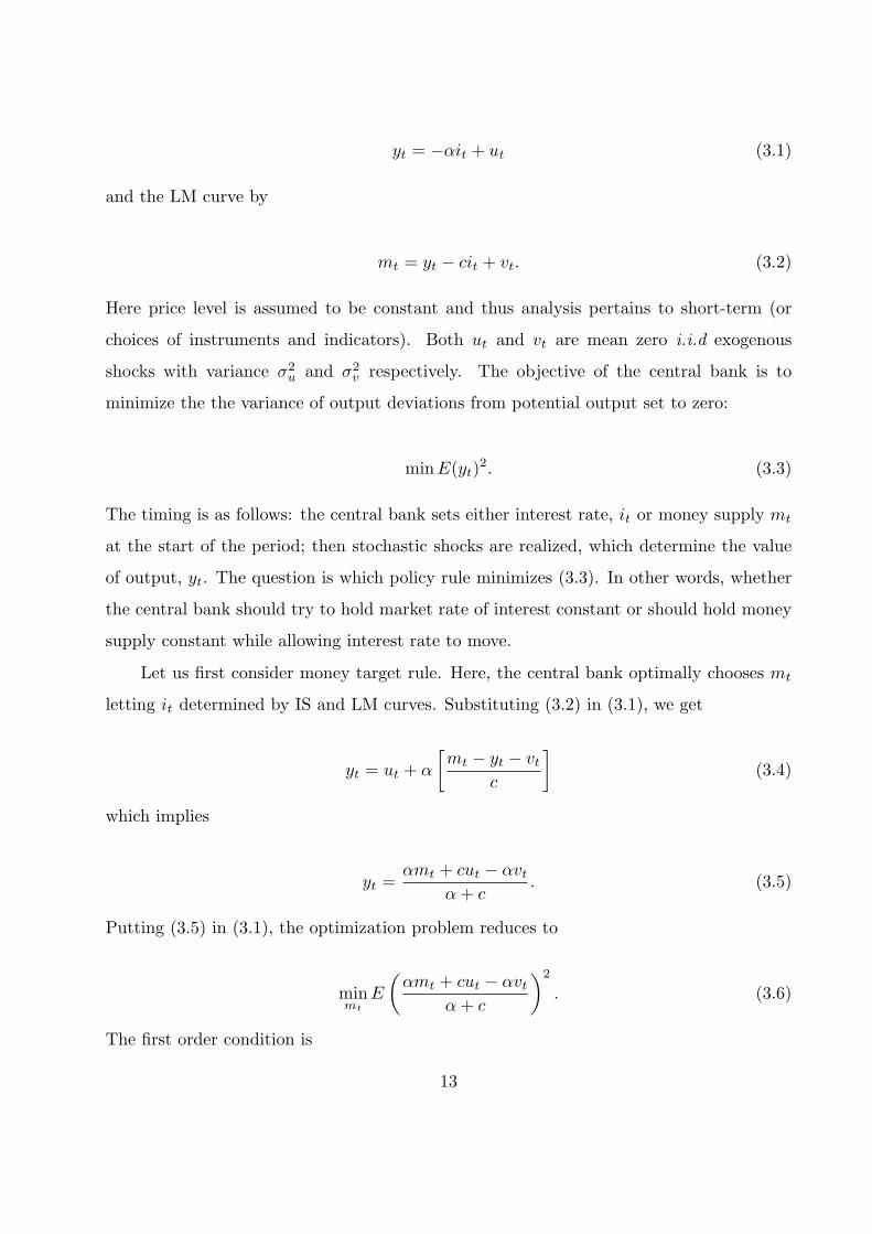
yt = −αit + ut (3.1)

and the LM curve by

mt = yt − cit + vt. (3.2)

Here price level is assumed to be constant and thus analysis pertains to short-term (or

choices of instruments and indicators). Both ut and vt are mean zero i.i.d exogenous

shocks with variance σ2u and σ2

v respectively. The objective of the central bank is to

minimize the the variance of output deviations from potential output set to zero:

min E(yt)2. (3.3)

The timing is as follows: the central bank sets either interest rate, it or money supply mt

at the start of the period; then stochastic shocks are realized, which determine the value

of output, yt. The question is which policy rule minimizes (3.3). In other words, whether

the central bank should try to hold market rate of interest constant or should hold money

supply constant while allowing interest rate to move.

Let us first consider money target rule. Here, the central bank optimally chooses mt

letting it determined by IS and LM curves. Substituting (3.2) in (3.1), we get

yt = ut + α

[mt − yt − vt

c

](3.4)

which implies

yt =αmt + cut − αvt

α + c. (3.5)

Putting (3.5) in (3.1), the optimization problem reduces to

minmt

E

(αmt + cut − αvt

α + c

)2

. (3.6)

The first order condition is

13

2E

(αmt + cut − αvt

α + c

)α

α + c= 0. (3.7)

From (3.7), we get optimal money supply rule as

mt = 0. (3.8)

With this policy rule, the value of objective function is

Em(yt)2 = Em

(cut − αvt

α + c

)2

=c2σ2

u + α2σ2v

(α + c)2. (3.9)

Let us now consider interest rate rule. Under this rule the central bank optimally

chooses it and allows money supply to adjust. In order to derive, optimal interest rate, it,

put (3.2), in (3.1). The optimization problem is now

minit

E(−αit + ut)2. (3.10)

From the first order condition, we get

it = 0. (3.11)

Putting (3.11) in the objective function, we have

Ei(yt)2 = σ2u. (3.12)

In order to find out optimal policy rule, we just have to compare (3.9) and (3.12). We

can immediately see that interest rate rule is preferred iff

Ei(yt)2 < Em(yt)2 (3.13)

which is equivalent to

σ2v >

(1 +

2c

α

)σ2

u. (3.14)

14

From (3.14) it is clear that if the only source of disturbance in the economy is money

market, σv > 0 & σu = 0, then the interest rule is preferred. In the case, the only source

of disturbance is goods market, σu > 0 & σv = 0, then the money supply rule is preferred.

If only good market shocks are present, a money rule leads to smaller variance in

output. Under interest rule, a positive IS shock leads to higher interest rate. This acts

to reduce aggregate spending, thereby partially the original shock. Since, the adjustment

of i automatically stabilizes output, preventing this interest rate adjustment by fixing i

leads to larger output fluctuations. If only money-demand shocks are present, output can

be stabilized perfectly by interest rate rule. Under a money rule, monetary shocks cause

the interest rate to move to maintain money market equilibrium, which causes output

fluctuations.

In the case, there is disturbances in both the markets, then the optimal policy rule

depends on size of variances as well as relative steepness of IS and LM curves. The interest

rate rule is more likely to be preferred when the variance of money market disturbances is

larger, the LM curve is steeper (lower c) and the IS curve is flatter (bigger α). Conversely,

the money supply rule is preferred if the variance of goods market shocks is large, the LM

curve is flat, and the IS curve is steeper.

Currently, Bank of Canada uses interest rate tool. It conducts its monetary policy by

announcing bank rate or operating band of overnight rate periodically. During 70’s and

80’s Bank of Canada used to target money supply. However, during 80’s the demand for

money function became highly unstable due to various financial innovations and Bank of

Canada abandoned monetary targeting and moved to interest rate targeting.

C. Taylor Rule

Many central banks including Bank of Canada and Federal Reserve conduct their

monetary policy through announcing bank rate or setting operating band for the overnight

rate. It raises the question, how central banks set the bank rate?

John Taylor showed that the behavior of the federal funds interest rate in the U.S.

from the mid-1980’s to 1992 could be fairly matched by a simple rule of the form

15

it = πt + 0.5(yt − yt) + 0.5(πt − πT ) + r∗ (3.15)

where πT was the target level of average inflation (assumed to be 2% per annum) and r∗

was the equilibrium level of real rate of interest (again assumed to be 2% per annum).

In the equation, the nominal interest rate deviates from the level consistent with the

economy’s equilibrium real rate and the target inflation rate if the output gap is nonzero

or if inflation deviates from target. A positive output gap leads to rise in nominal interest

rate as does actual inflation higher than the target level.

The Taylor rule for general coefficients is often written as

it = r∗ + πT + α(yt − yt) + β(πt − πT ). (3.16)

A large literature has developed that has estimated Taylor rule for different countries and

time-periods. The rule does quite well to match the actual behavior of overnight rates,

when supplemented by the addition of lagged nominal interest rate.

D. Uncertainty About the Impact of Policy Instruments or Model Uncertainty

So far we have assumed that the central bank knows the true model of the economy

with certainty or knows the true impact of its policy. Fluctuations in output and inflation

arose from disturbances that took the form of additive errors. But suppose that the central

bank does not know the true model with certainty or measures parameter values with error.

In other words, the error terms enter multiplicatively. In this case, it may be optimal for

the central bank to respond to shocks more slowly or cautiously.

To concretize this idea, suppose that the central bank’s objective function is

L =12Et(π2

t + λy2t ). (3.17)

Here for simplicity, I have assumed that social welfare maximizing output, y∗t and inflation,

π∗t are zero. Now suppose that aggregate demand evolves as follows

yt = βtπt + et (3.18)

16

where et is mean zero i.i.d. shock. Also assume that the central bank does not know the

true βt, but has to rely on estimated βt. The true β is related to estimated β as follows

βt = β + vt (3.19)

where vt is mean zero i.i.d. shock with variance σ2v and β is the true parameter. Now

suppose that the central bank observes demand shock et but not vt before choosing πt.

Now the question is: what is the optimal πt?

To derive optimal πt, put (3.18) in (3.17), then we have

minπt

=12Et

[π2

t + λ(βtπt + et)2]. (3.20)

The first order condition is

Et(πt + λ(βtπt + et)βt) = 0. (3.21)

Simplifying, we have

πt = − λβ

1 + β2

+ σ2v

et. (3.22)

As one can see that the coefficient of demand shock et is declining in σ2v . This basically

says that in the presence of multiplicative disturbances, it is optimal for the central bank

to respond less (or more cautiously) to et.

4. Time Inconsistency and Targeting Rules

Empirical literature suggests that inflation is mainly accounted for by the increase in

money supply at least in medium and long run. Given that inflation is costly, it raises

the question, why the governments follow inflationary policy or expansionary monetary

policy? One reason can be that the increase in money supply is a source of revenue for

the government (seniorage). However, this explanation does not seem to very appropriate

for the developed countries, where government revenue from money creation is not very

important.

17

The other explanation is that output-inflation trade-off faced by the central banks

induces them to pursue expansionary policy. When output is low, they may be tempted

to increase inflation. On the other hand, when inflation is high, they may be reluctant to

reduce it for the fear of reducing output. However, this explanation as stated also falls

short because there is no long run trade-off between output and inflation. If there is no

long-run tarde-off, why do we observe long run inflation?

Kydland and Presscott (1977) in a famous paper showed that when the central banks

have discretion to set inflation and if they only face short-run output-inflation trade-off,

then it gives rise to excessively expansionary policy. Intuitively, when expected inflation is

low, the marginal cost of additional inflation is low. This induces central banks to increase

inflation (for a given expected inflation), in order to increase output. However, the public

while forming their expectation take into account the incentives of the central bank and

thus do not expect low inflation. In other words, the promise of central bank to follow

low inflation is not credible. Consequently, central banks’ discretion results in inflation

without any increase in output.

A. Time Inconsistency

Lack of credibility of central bank’s low inflation policy gives rise to the problem of

dynamic inconsistency of low inflation monetary policy. Idea is that the central bank

would like public to believe that it will follow low inflation policy i.e. it will announce low

inflation target. However, once the public has formed their expectation based on central

bank’s announcement, the central bank has incentive to increase inflation as by doing so

it can increase output. Since, the central bank does not comply with its announcement,

its announcement is not time-consistent. In other words, at the time of choosing actual

inflation, the central bank deviates from its inflation target. Let us now formalize these

ideas.

Let the objective function of the central bank be

L =12λ(yt − y − k)2 +

12(πt − π∗)2 (4.1)

18

where y is the potential output, k is some constant, and π∗ is socially optimal inflation rate.

Here y + k stands for socially optimal output level. The deviation in the socially optimum

level of output and potential output can be due to distortionary taxes or imperfections in

markets.

Let the trade-off between inflation and output be given by

yt = y + a(πt − πet ). (4.2)

(4.2) is the Lucas supply curve which we discussed in chapter 1. The central chooses actual

inflation, πt, in order to minimize (4.1) subject to (4.2).

Now suppose the timing of events are as follows. The central bank first announces

its target inflation rate. After the announcement of the central bank, public form their

expectation about inflation rationally. Once public has formed its expectation, the central

bank chooses actual inflation. The key here is that the central bank chooses actual inflation

after public have formed their expectation.

Given the environment, we need to answer two questions: (i) what is the actual

inflation chosen by the central bank? (ii) what is the expected inflation? We will answer

these two questions under two policies – (i) full commitment and (ii) discretion. By full

commitment, we mean that the central bank adheres to its announcement. By discretion,

we mean that the central bank can choose actual inflation different from the announced

one.

Now under the full commitment, the socially optimal policy is

πt = π∗ = πet . (4.3)

The value of objective function is

Lc =12λk2. (4.4)

Under discretion, the optimal, πt, can be derived as follows. Putting (4.2) in (4.1),

we have

19

minπt

12λ(a(πt − πe

t )− k)2 +12(πt − π∗)2. (4.5)

The first order condition yields,

λ(a(πt − πet )− k)a = (π∗ − πt). (4.6)

Under rational expectation and no uncertainty, πet = πt and thus (4.6) becomes

−λak = π∗ − πt (4.7)

which simplifies to

πt = π∗ + λak. (4.8)

Time-consistent inflation, πt, is higher than the socially optimum inflation rate, π∗, and

the size of inflation bias is λak. The value of objective function under time-consistent

policy is

Ld =12λk2 +

12(λak)2 (4.9)

which is higher than value of the objective function under full commitment. In other

words, the economy does worse-off under discretion.

Many solutions have been proposed to address the problem of time-inconsistency. One

set of solution is to target some nominal variable – money supply, exchange rate, nominal

income, price level, inflation etc. Next we turn to analyze inflation targeting.

B. Inflation-Targeting

Inflation targeting basically involves announcing an inflation target and increasing the

weight of deviation of actual inflation from targeted inflation in the social welfare function.

The idea of inflation targeting can be captured as follows.

Suppose that the target inflation rate is equal to the optimal inflation rate. Let the

objective function of the central bank be

20

V =12λ(yt − y − k)2 +

12(πt − π∗)2 +

12h(πt − π∗)2. (4.10)

The last term in (4.10) is the additional penalty on the central bank. If h = 0, we go back

to the original case. The problem of the central bank is to choose inflation rate πt in order

to minimize (4.10) subject to (4.2). Now under the full commitment, the socially optimal

policy is still

πt = π∗. (4.11)

Under inflation-targeting regime, the optimal, πt, can be derived as follows. Putting (4.2)

in (4.10), we have

minπt

12λ(a(πt − πe)− k)2 +

12(πt − π∗)2 +

12h(πt − π∗)2. (4.12)

The first order condition yields,

λ(a(πt − πe)− k)a = (π∗ − πt)− h(πt − π∗t ). (4.13)

Under rational expectation, πt = πet and thus (4.13) becomes

−λak = (1 + h)π∗ − (1 + h)πt (4.14)

which simplifies to

πt = π∗ +λak

1 + h. (4.15)

By comparing (4.15) with (4.8), we can immediately see that the size of inflation bias is

smaller under inflation targeting.

21