Module1

Numerical Solution of Ordinary Differential Equations

Lecture 4

Runge Kutta Method

Keywords: one step algorithm, Taylor series, Runge-Kutta method

Runge Kutta Method

The solution of differential equation with desired accuracy can be achieved using

classical Taylor series method at a specified point. This means for given h, one can go

on adding more and more terms of the series till the desired accuracy is achieved. This

requires the expressions for several higher order derivatives and its evaluation. It poses

practical difficulties in the application of Taylor series method:

Higher order derivatives may not be easily obtained

Even if the expressions for derivatives are obtained, lot of computational effort may

still be required in their numerical evaluation

It is possible to develop one step algorithms which require evaluation of first derivative

as in Euler method but yields accuracy of higher order as in Taylor series. These

methods require functional evaluations of f(t,y(t)) at more than one point.on the interval

[tk,tk+1]. The Category of methods are known as Runge-Kutta methods of order 2, 3 and

more depending upon the order of accuracy. .A general Runge Kutta algorithm is given

as

( , , )k 1 k k ky y h t y h (1.7)

The function phi is termed as increment function. The mth order Runge-Kutta method

gives accuracy of order hm. The function is chosen in such a way so that when

expanded the right hand side of (1.7) matches with the Taylor series upto desired order.

This means that for a second order Runge-Kutta mehod the right side of (1.7 ) matches

up to second order terms of Taylor series.

Second Order Runge Kutta Methods

The Second order Runge Kutta methods are known as RK2 methods. For the derivation

of second order Runge Kutta methods, it is assumed that phi is the weighted average of

two functional evaluations at suitable points in the interval [tk,tk+1]:

( , , )

( , )

( , ); ,

k k 1 1 2 2

1 k k

2 k k 1

t y h w K w K

K f t y

K f t ph y qhK 0 p q 1

(1.8)

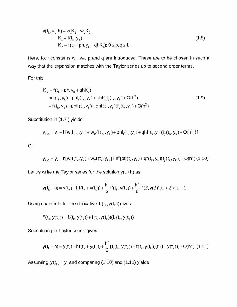
Here, four constants w1, w2, p and q are introduced. These are to be chosen in such a

way that the expansion matches with the Taylor series up to second order terms.

For this

( , )

( , ) ( , ) ( , ) ( )

( , ) ( , ) ( , )( ( , ) ( )

2 k k 1

2k k t k k 1 y k k

2k k t k k k k y k k

K f t ph y qhK

f t y phf t y qhK f t y O h

f t y phf t y qhf t y f t y O h

(1.9)

Substitution in (1.7 ) yields

[ ( , ) { ( , ) ( , ) ( , )( ( , ) ( )}]2

k 1 k 1 k k 2 k k t k k k k y k ky y h w f t y w f t y phf t y qhf t y f t y O h

Or

 [ ( , ) ( , )] [ ( , ) ( , )( ( , )] ( )2 3

k 1 k 1 k k 2 k k t k k k k y k ky y h w f t y w f t y h pf t y qf t y f t y O h (1.10)

Let us write the Taylor series for the solution y(tk+h) as

( ) ( ) ( ( )) ( , ( )) ( , ( ));2 3

k k k k k k k k

h hy t h y t hf t y t f t y t f y t t 1

2 6

Using chain rule for the derivative ( , ( ))k kf t y t gives

( , ( )) ( , ( )) ( , ( ))( ( , ( ))k k t k k k k y k kf t y t f t y t f t y t f t y t

Substituting in Taylor series gives

( ) ( ) ( ( )) [ ( , ( )) ( , ( ))( ( , ( ))] ( )2

3k k k k t k k k k y k k

hy t h y t hf t y t f t y t f t y t f t y t O h

2 (1.11)

Assuming ( )k ky t y and comparing (1.10) and (1.11) yields

, / /1 2 1 2w w 1 w p 1 2 and w q 1 2 (1.12)

Observe that four unknowns are to be evaluated from three equations. Accordingly

many solutions are possible for (1.12). Let us chose arbitrary value to constant q as

q=1, then

/ ,1 2w w 1 2 p 1 and q 1

Accordingly, the second order Runge-Kutta can be written as

( , )

[ ( , ) ( , )]

kp k k k

k 1 k k k k kp

y y hf t y

hy y f t y f t h y

2

(1.13)

This is the same as modified Euler method. It may be noted that the method reduces to

a quadrature formula [Trapezoidal rule] when f(t, y) is independent of y:

[ ( ) ( )] k 1 k k k

hy y f t f t h

2

For convenience q is chosen between 0 and 1such that one of the weights w in the

method is zero. For example choose q=1/2 makes w1=0 and (1.12) yields:

, , /1 2w 0 w 1 p q 1 2

( , )

( , )

k k k k

k 1 k k k

hy y f t y

2h

y y hf t y2

(1.14)

Choosing arbitrary constant q so as to minimize the sum of absolute values of

coefficients in the truncation error term Tj+1 gives optimal RK method. The minimum

error occurs for q=2/3. Accordingly optimal method is obtained for

/ , / , /1 2w 1 4 w 3 4 p q 2 3

This gives another second order Runge-Kutta method known as optimal RK2 method:

( , )

( , ) ( , )

k k k k

k 1 k k k k k

2hy y f t y

3h 3h 2h

y y f t y f t y4 4 3

(1.15)

Example 1.5: Solve IVP in 1<t<2 with h=0.1using Optimal Runge Kutta Method (1.15)

/ ( / ) ; ( ) 2y y t y t y 1 1

Solution: The solution is given in table 1.3

t yk f(t,y) yk0 t+2h/3 f(t+2h/3,yk0) yk+1

1 1 0 1 1.066667 0.05859375 1.004395

1.1 1.004395 0.07936 1.020267 1.166667 0.119744262 1.015359

1.2 1.015359 0.130192 1.041398 1.266667 0.159037749 1.030542

1.3 1.030542 0.164312 1.063404 1.366667 0.185456001 1.048559

1.4 1.048559 0.188014 1.086162 1.466667 0.203806563 1.068545

1.5 1.068545 0.204902 1.109525 1.566667 0.216857838 1.089932

1.6 1.089932 0.217164 1.133364 1.666667 0.226296619 1.112333

1.7 1.112333 0.226187 1.157571 1.766667 0.233198012 1.135478

1.8 1.135478 0.232886 1.182055 1.866667 0.238272937 1.15917

1.9 1.15917 0.23788 1.206746 1.966667 0.242006106 1.183268

2 1.183268 0.241603 1.231588 2.066667 0.244736661 1.207663

Table 1.3: Solution of Example 1.5 with h=0.1

[Ref modified-euler.xlsx/sheet3]