Embed Size (px)
Citation preview
1
Lecture 3 The wave equation
Mathématiques appliquées (MATH0504-1)B. Dewals, C. Geuzaine
01/10/2021
2
Learning objectives of this lecture
Understand the fundamental properties of the wave equation
Write the general solution of the wave equation
Solve initial value problems with the wave equation
Understand the concepts of causality, domain of influence, and domain of dependence in relation with the wave equation
Become aware that the wave equation ensures conservation of energy
3
Outline
1. Reminder: physical significance and derivation of the wave equation, basic properties
2. General solution of the wave equation
3. Initial value problem
4. Causality
5. Energy
6. Generalized wave equation

4
1 - Reminders
5
Reminder
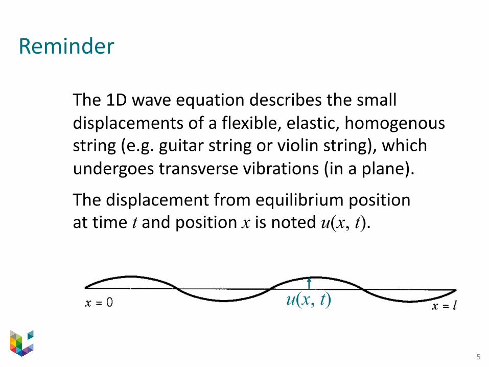
The 1D wave equation describes the small displacements of a flexible, elastic, homogenous string (e.g. guitar string or violin string), which undergoes transverse vibrations (in a plane).
The displacement from equilibrium position at time t and position x is noted u(x, t).
u(x, t)
6
Reminder
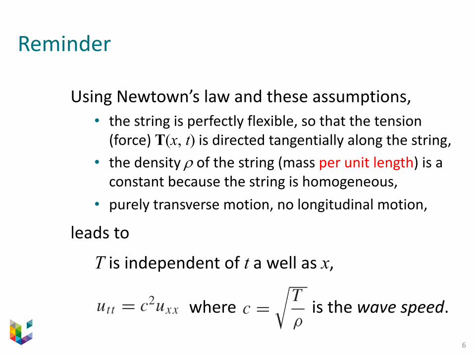
Using Newtown’s law and these assumptions,• the string is perfectly flexible, so that the tension
(force) T(x, t) is directed tangentially along the string,• the density r of the string (mass per unit length) is a
constant because the string is homogeneous,• purely transverse motion, no longitudinal motion,
leads to
T is independent of t a well as x,
where is the wave speed.
7
Reminder
The 1D wave equation, or a variation of it, describes also other wavelike phenomena, such as
• vibrations of an elastic bar, • sound waves in a pipe,• long water waves in a straight channel,• the electrical current in a transmission line …
The 2D and 3D versions of the equation describe:• vibrations of a membrane / of an elastic solid, • sound waves in air, • electromagnetic waves (light, radar, etc.), • seismic waves propagating through the earth …
8
For the sake of simplification, we consider herean infinite domain: −∞ < x < +∞
Real physical situations are often on finite intervals.
However, we do not consider boundaries here,for two reasons:
• from a mathematical perspective, the absence of a boundary is a big simplification, which does not prevent shedding light on most of the fundamental properties of PDEs;
• from a physical perspective, far away from the boundary, it will take a certain time for the boundary to have a substantial effect on the process, and until that time the solutions derived here are valid.
9
Basic properties of the wave equation
The wave equation (WE) writes:
where the following notation is used for the derivatives: …
The WE has the following basic properties:• it has two independent variables, x and t,
and one dependent variable u(i.e. u is an unknown function of x and t);
• it is a second-order PDE, since the highest derivative in the equation is second order;
• it is a homogeneous linear PDE.
10
The wave equation is a hyperbolic PDE
Comparing the wave equation
to the general formulation
reveals that
since a12 = 0, a11 = ‒ c2 and a22 = 1.
Hence, the wave equation is hyperbolic.

11
2 – Solution of the wave equationIn this section, we use two different approaches to derive the general solution of the wave equation (Section 2.1 in Strauss, 2008).
12
1st approach The operator in the wave equation factors
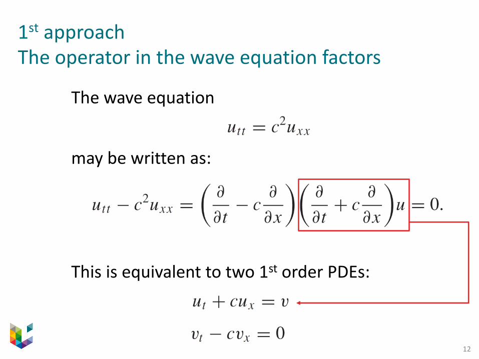
The wave equation
may be written as:
This is equivalent to two 1st order PDEs:
13
1st approach We solve each of the two 1st order PDEs
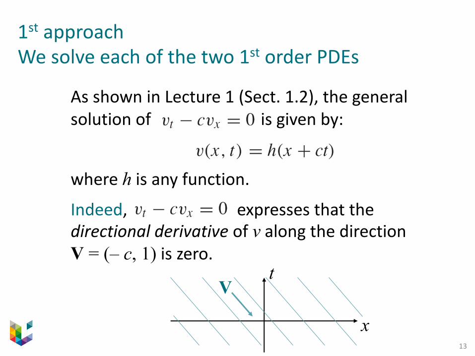
As shown in Lecture 1 (Sect. 1.2), the general solution of is given by:
where h is any function.
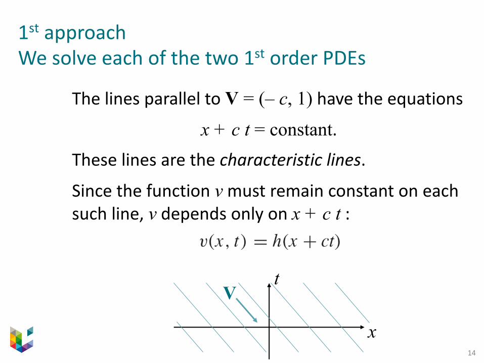
Indeed, expresses that the directional derivative of v along the direction V = (‒ c, 1) is zero.
x
tV
14
1st approach We solve each of the two 1st order PDEs
The lines parallel to V = (‒ c, 1) have the equations
x + c t = constant.These lines are the characteristic lines.
Since the function v must remain constant on each such line, v depends only on x + c t :
x
tV
15
1st approach We solve each of the two 1st order PDEs
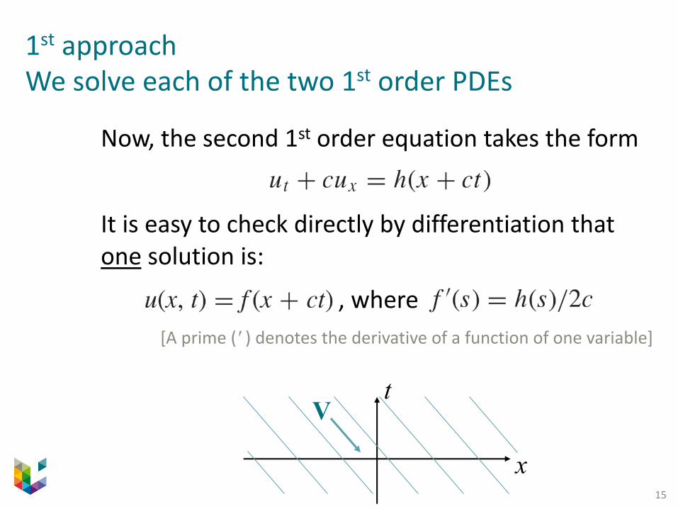
Now, the second 1st order equation takes the form
It is easy to check directly by differentiation that one solution is:
, where[A prime (ʹ ) denotes the derivative of a function of one variable]
x
tV
16
1st approach We solve each of the two 1st order PDEs
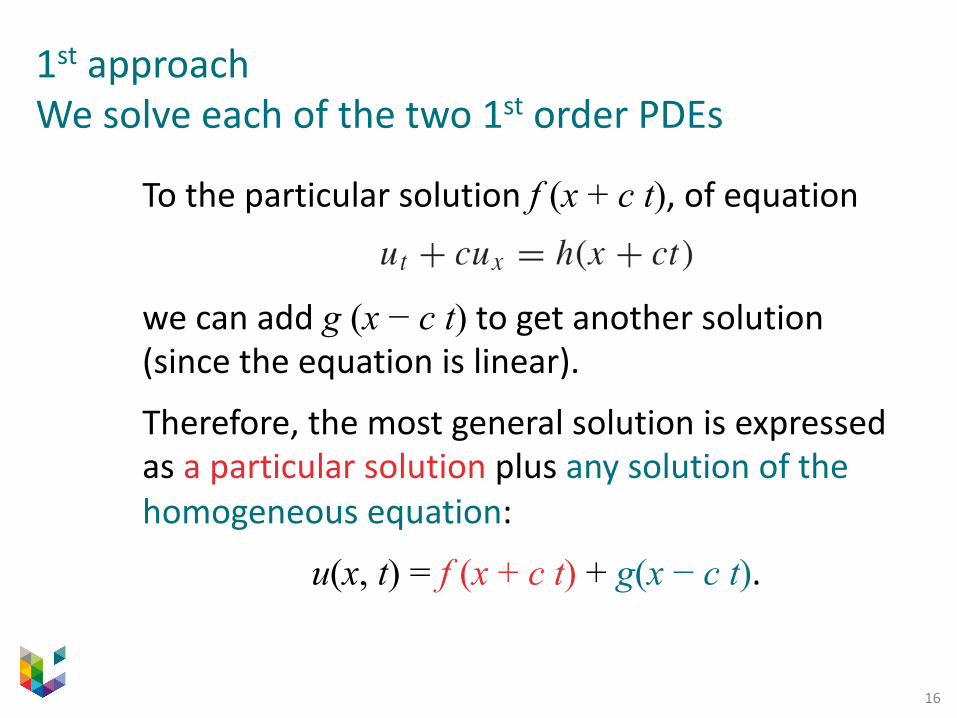
To the particular solution f (x + c t), of equation
we can add g (x − c t) to get another solution (since the equation is linear).
Therefore, the most general solution is expressed as a particular solution plus any solution of the homogeneous equation:
u(x, t) = f (x + c t) + g(x − c t).
17
2nd approach Introduce the characteristic coordinates
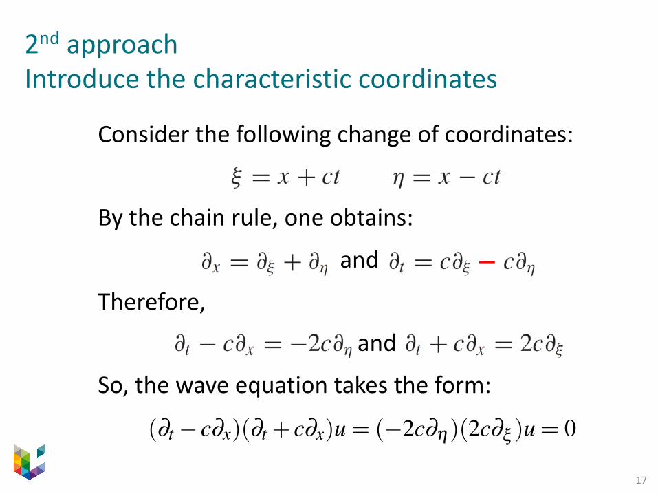
Consider the following change of coordinates:
By the chain rule, one obtains:
and
Therefore,
and
So, the wave equation takes the form:
−
(∂t � c∂x)(∂t + c∂x)u = (�2c∂h)(2c∂x )u = 0
18
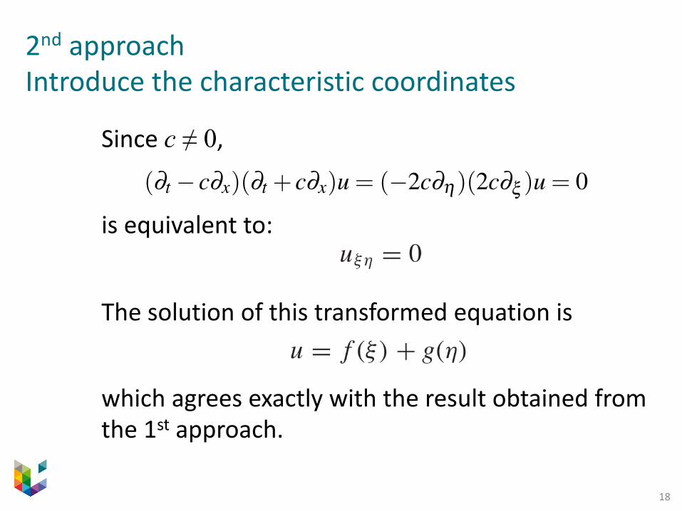
2nd approach Introduce the characteristic coordinates
Since c ≠ 0,
is equivalent to:
The solution of this transformed equation is
which agrees exactly with the result obtained from the 1st approach.
(∂t � c∂x)(∂t + c∂x)u = (�2c∂h)(2c∂x )u = 0
19
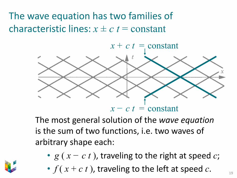
The most general solution of the wave equationis the sum of two functions, i.e. two waves of arbitrary shape each:• g ( x − c t ), traveling to the right at speed c; • f ( x + c t ), traveling to the left at speed c.
The wave equation has two families of characteristic lines: x ± c t = constant
x − c t = constant
x + c t = constant

20
Here, we anticipate the result of a numeric example detailed later on …
+
21
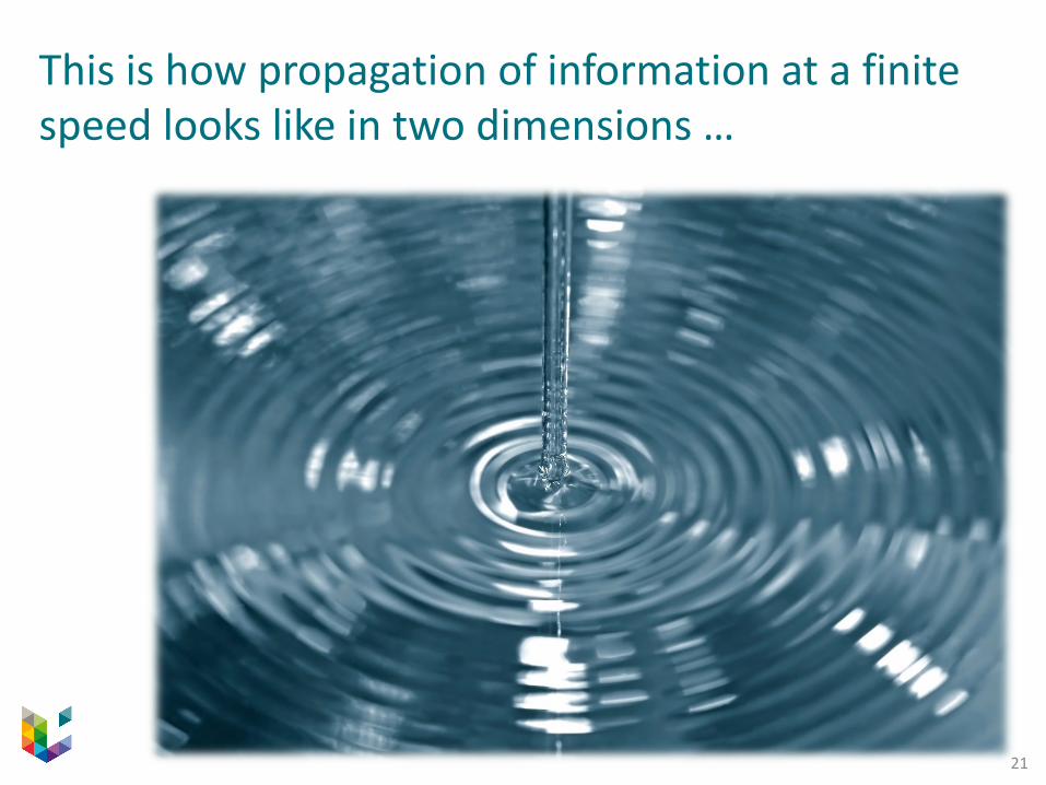
This is how propagation of information at a finite speed looks like in two dimensions …

23
3 – Initial value problemIn this section, we solve the initial value problem and present a few worked out examples(Section 2.1 in Strauss, 2008)
24
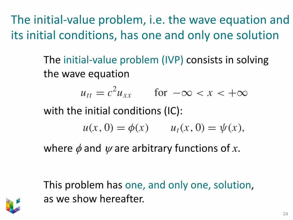
The initial-value problem, i.e. the wave equation and its initial conditions, has one and only one solution
The initial-value problem (IVP) consists in solving the wave equation
with the initial conditions (IC):
where f and y are arbitrary functions of x.
This problem has one, and only one, solution,as we show hereafter.
25
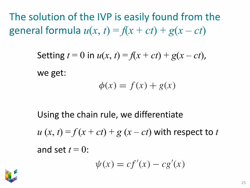
The solution of the IVP is easily found from the general formula u(x, t) = f(x + ct) + g(x – ct)
Setting t = 0 in u(x, t) = f(x + ct) + g(x – ct),
we get:
Using the chain rule, we differentiate
u (x, t) = f (x + ct) + g (x – ct) with respect to t
and set t = 0:
26
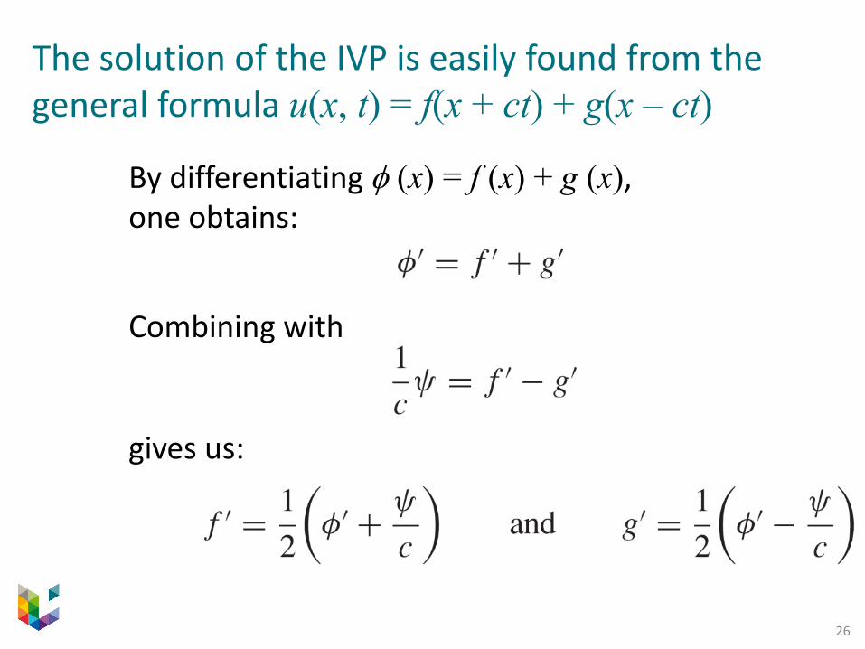
The solution of the IVP is easily found from the general formula u(x, t) = f(x + ct) + g(x – ct)
By differentiating f (x) = f (x) + g (x), one obtains:
Combining with
gives us:
27
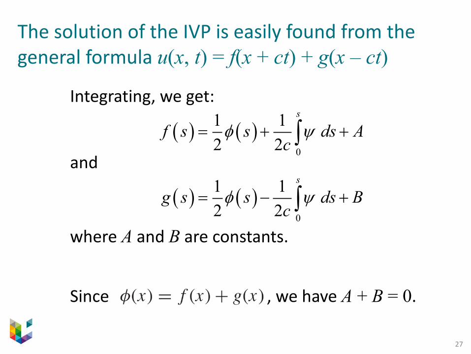
The solution of the IVP is easily found from the general formula u(x, t) = f(x + ct) + g(x – ct)
Integrating, we get:
and
where A and B are constants.
Since , we have A + B = 0.
( ) ( )0
1 12 2
s
f s s ds Ac
f y= + +ò
( ) ( )0
1 12 2
s
g s s ds Bc
f y= - +ò
28
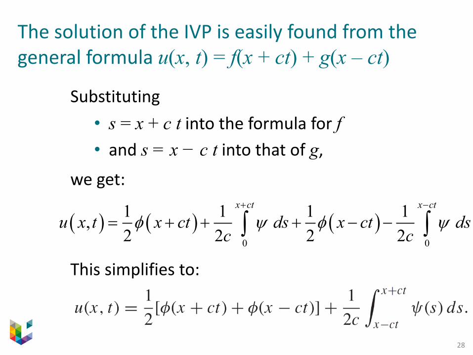
The solution of the IVP is easily found from the general formula u(x, t) = f(x + ct) + g(x – ct)
Substituting • s = x + c t into the formula for f• and s = x − c t into that of g,
we get:
This simplifies to:
( ) ( ) ( )0 0
1 1 1 1,2 2 2 2
x ct x ct
u x t x ct ds x ct dsc c
f y f y+ -
= + + + - -ò ò
29
A first worked out example
Considering f (x) = sin x and y (x) = 0, one obtains from the general solution:
u(x, t) = [ sin ( x + c t ) + sin ( x – c t ) ] / 2Hence,
u(x, t) = sin x cos ( c t ).This can be checked easily by substituting the expression found for u(x, t) into the wave equation.
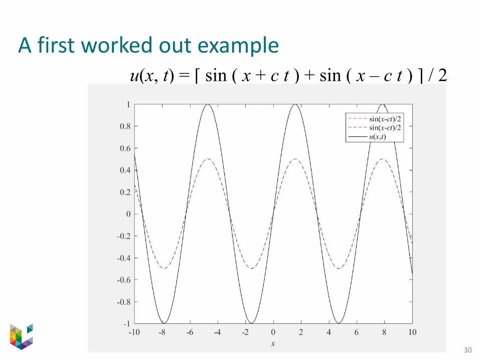
30
A first worked out exampleu(x, t) = [ sin ( x + c t ) + sin ( x – c t ) ] / 2
+
31
Another example
Let us consider now f (x) = 0 and y (x) = cos x.
The solution writes:
u(x, t) = [ sin ( x + c t ) ‒ sin ( x – c t ) ] / ( 2 c )Hence,
u(x, t) = cos x sin ( c t ) / c .Again, this can be checked easily by substituting the result into the wave equation and the IC.
32
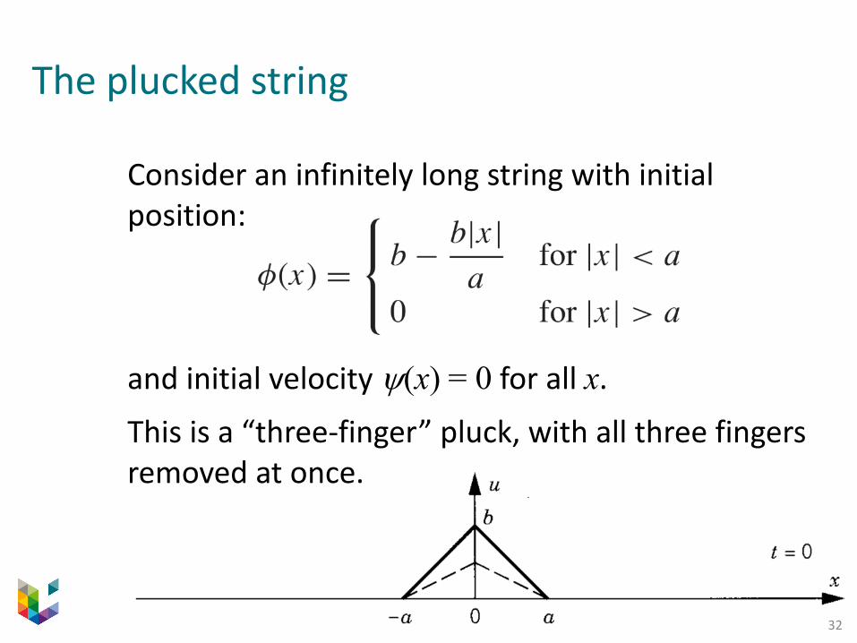
The plucked string
Consider an infinitely long string with initial position:
and initial velocity y(x) = 0 for all x.
This is a “three-finger” pluck, with all three fingers removed at once.
33
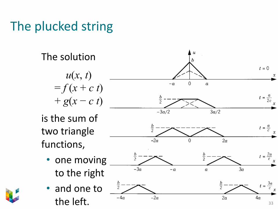
The plucked string
The solution
u(x, t) = f (x + c t) + g(x − c t)
is the sum of two triangle functions,• one moving
to the right • and one to
the left.
34
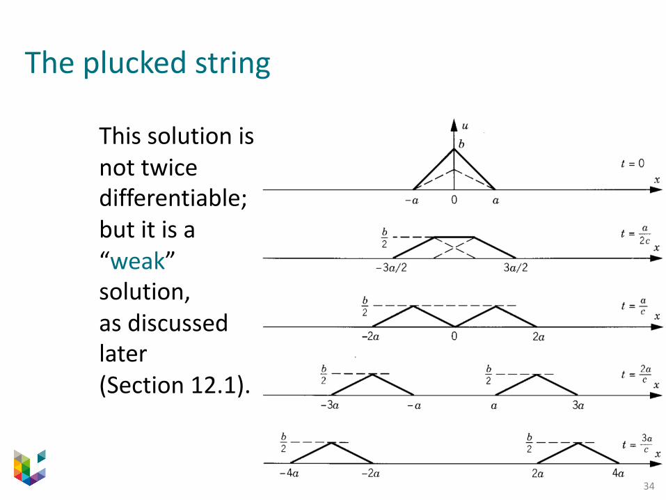
The plucked string
This solution is not twice differentiable; but it is a “weak” solution, as discussed later (Section 12.1).
35
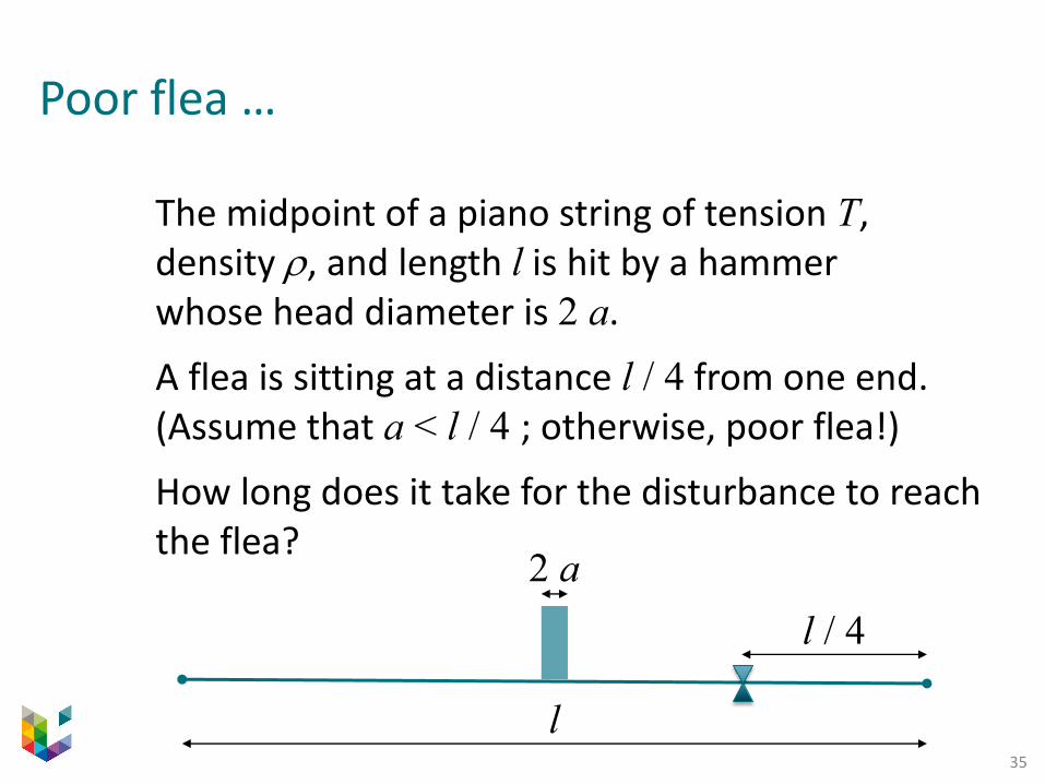
Poor flea …
The midpoint of a piano string of tension T, density r, and length l is hit by a hammer whose head diameter is 2 a.
A flea is sitting at a distance l / 4 from one end. (Assume that a < l / 4 ; otherwise, poor flea!)
How long does it take for the disturbance to reach the flea?
l
2 al / 4
36
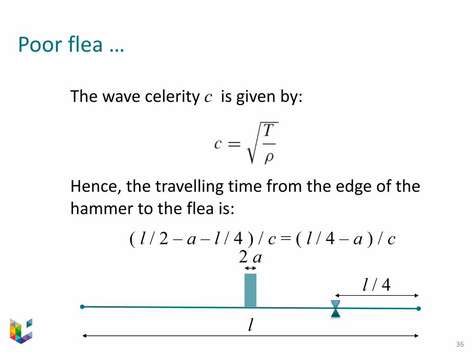
Poor flea …
The wave celerity c is given by:
Hence, the travelling time from the edge of the hammer to the flea is:
( l / 2 – a – l / 4 ) / c = ( l / 4 – a ) / c
l
2 al / 4

39
4 – Causality in the wave equationIn this section, we introduce the concepts of zones of influence and of dependence (Section 2.2 in Strauss, 2008)
40
Principle of causality: no part of the waves goes faster than speed c
We have just learned that • the effect of an initial position f(x) is a pair of
waves traveling in either direction at speed cand at half the original amplitude;
• the effect of an initial velocity y(x) is a wave spreading out at speed ≤ c in both directions.
So, part of the wave may lag behind (if there is an initial velocity), but
no part goes faster than speed c.
This is the principle of causality.
43
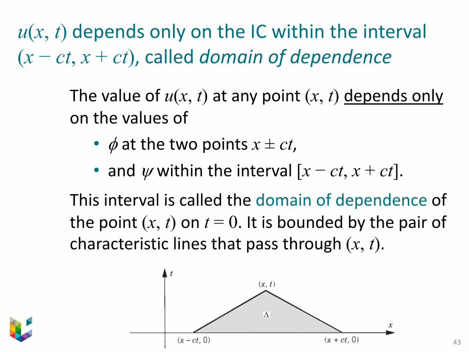
u(x, t) depends only on the IC within the interval (x − ct, x + ct), called domain of dependence
The value of u(x, t) at any point (x, t) depends onlyon the values of • f at the two points x ± ct, • and y within the interval [x − ct, x + ct].
This interval is called the domain of dependence of the point (x, t) on t = 0. It is bounded by the pair of characteristic lines that pass through (x, t).
44
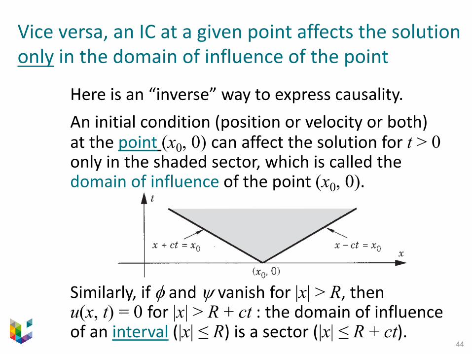
Vice versa, an IC at a given point affects the solution only in the domain of influence of the point
Here is an “inverse” way to express causality. An initial condition (position or velocity or both) at the point (x0, 0) can affect the solution for t > 0 only in the shaded sector, which is called the domain of influence of the point (x0, 0).
Similarly, if f and y vanish for |x| > R, then u(x, t) = 0 for |x| > R + ct : the domain of influence of an interval (|x| ≤ R) is a sector (|x| ≤ R + ct).

45
5 – Energy in the wave equationIn this section, we demonstrate that the wave equation ensures conservation of energy (Section 2.2 in Strauss, 2008)
46
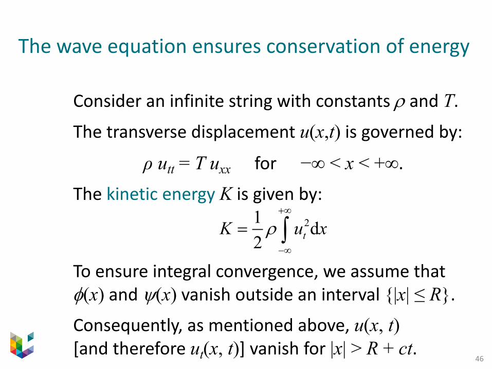
The wave equation ensures conservation of energy
Consider an infinite string with constants r and T.
The transverse displacement u(x,t) is governed by:
ρ utt = T uxx for −∞ < x < +∞.
The kinetic energy K is given by:
To ensure integral convergence, we assume that f(x) and y(x) vanish outside an interval {|x| ≤ R}.
Consequently, as mentioned above, u(x, t)[and therefore ut(x, t)] vanish for |x| > R + ct.
21 d2 tK u xr
+¥
-¥
= ò
47
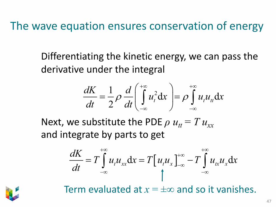
The wave equation ensures conservation of energy
Differentiating the kinetic energy, we can pass the derivative under the integral
Next, we substitute the PDE ρ utt = T uxxand integrate by parts to get
21 d d2 t t tt
dK d u x u u xdt dt
r r+¥ +¥
-¥ -¥
æ ö= =ç ÷
è øò ò
[ ]d dt xx t x tx xdK T u u x T u u T u u xdt
+¥ +¥+¥
-¥-¥ -¥
= = -ò ò
Term evaluated at x = ±∞ and so it vanishes.
48
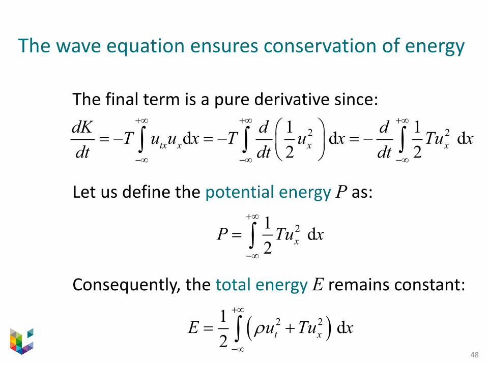
The wave equation ensures conservation of energy
The final term is a pure derivative since:
Let us define the potential energy P as:
Consequently, the total energy E remains constant:
2 21 1d d d2 2tx x x x
dK d dT u u x T u x Tu xdt dt dt
+¥ +¥ +¥
-¥ -¥ -¥
æ ö= - = - = -ç ÷è øò ò ò
21 d2 xP Tu x
+¥
-¥
= ò
( )2 21 d2 t xE u Tu xr
+¥
-¥
= +ò

49
4 – GeneralizationThrough one example, we show here that a range of more general equations can be solved in a similar way as the wave equation discussed so far.
50
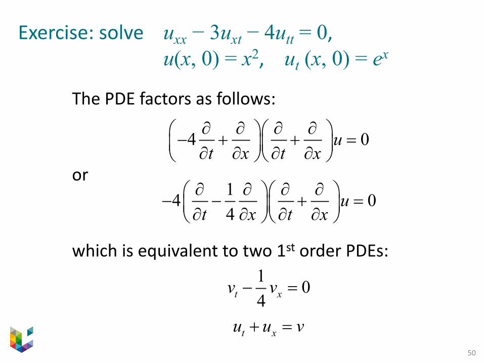
Exercise: solve uxx − 3uxt − 4utt = 0, u(x, 0) = x2, ut (x, 0) = ex
The PDE factors as follows:
or
which is equivalent to two 1st order PDEs:
4 0ut x t x¶ ¶ ¶ ¶æ öæ ö- + + =ç ÷ç ÷¶ ¶ ¶ ¶è øè ø
t xu u v+ =
1 04t xv v- =
14 04
ut x t x¶ ¶ ¶ ¶æ öæ ö- - + =ç ÷ç ÷¶ ¶ ¶ ¶è øè ø
51
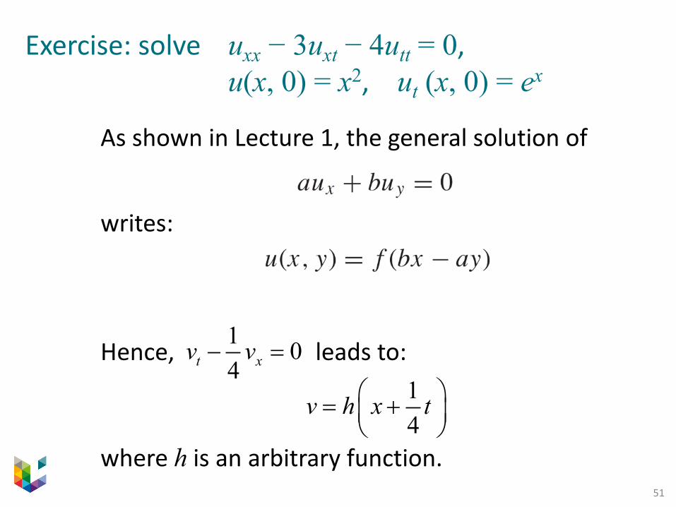
Exercise: solve uxx − 3uxt − 4utt = 0, u(x, 0) = x2, ut (x, 0) = ex
As shown in Lecture 1, the general solution of
writes:
Hence, leads to:
where h is an arbitrary function.
14
v h x tæ ö= +ç ÷è ø
1 04t xv v- =
52
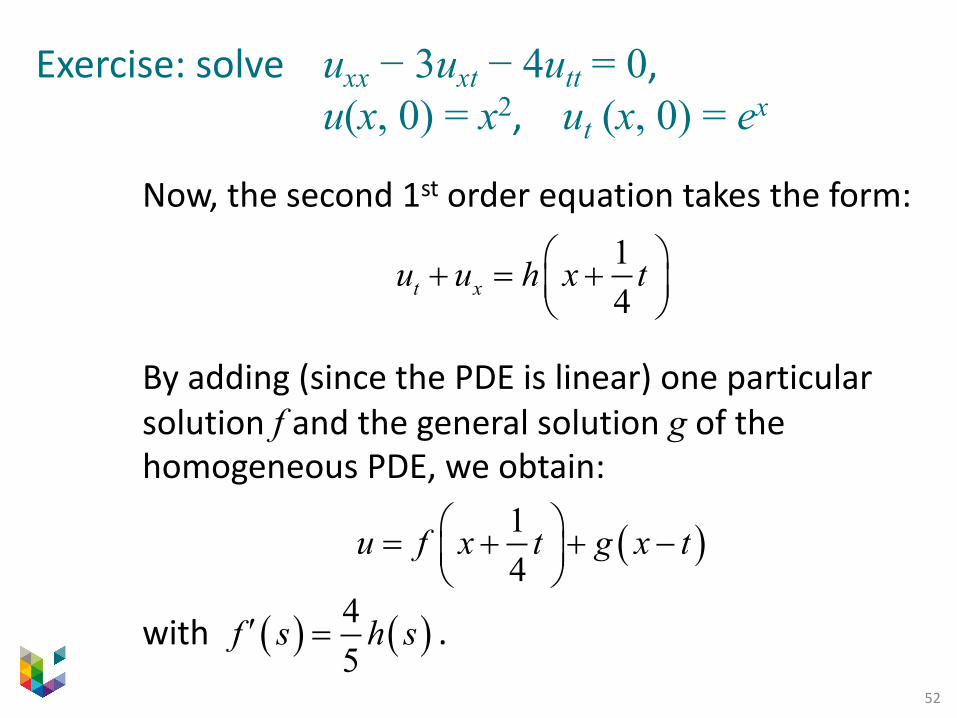
Exercise: solve uxx − 3uxt − 4utt = 0, u(x, 0) = x2, ut (x, 0) = ex
Now, the second 1st order equation takes the form:
By adding (since the PDE is linear) one particular solution f and the general solution g of the homogeneous PDE, we obtain:
with .
14t xu u h x tæ ö+ = +ç ÷
è ø
( )14
u f x t g x tæ ö= + + -ç ÷è ø
( ) ( )45
f s h s¢ =
53
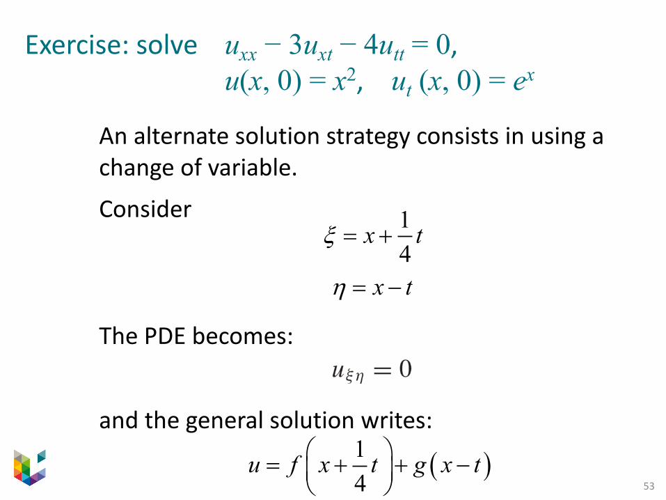
Exercise: solve uxx − 3uxt − 4utt = 0, u(x, 0) = x2, ut (x, 0) = ex
An alternate solution strategy consists in using a change of variable.
Consider
The PDE becomes:
and the general solution writes:
14
x tx = +
x th = -
( )14
u f x t g x tæ ö= + + -ç ÷è ø
54
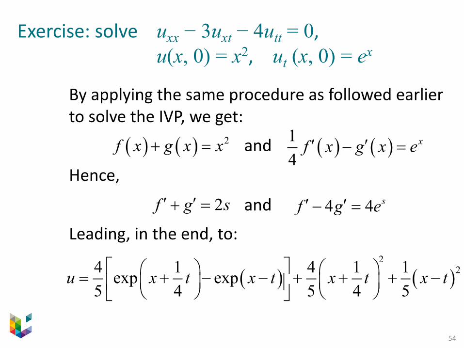
Exercise: solve uxx − 3uxt − 4utt = 0, u(x, 0) = x2, ut (x, 0) = ex
By applying the same procedure as followed earlier to solve the IVP, we get:
and
Hence,
and
Leading, in the end, to:
( ) ( ) 2f x g x x+ =
( ) ( )2
24 1 4 1 1exp exp5 4 5 4 5
u x t x t x t x té ùæ ö æ ö= + - - + + + -ç ÷ ç ÷ê úè ø è øë û
2f g s¢ ¢+ =
( ) ( )14
xf x g x e¢ ¢- =
4 4 sf g e¢ ¢- =
55
Take-home messages
The basic properties of the wave equation include:• the IVP has one, and only one, solution,• information gets transported in both directions
(along the characteristic lines) at a finite speed, • consequently, an initial condition at a given
point affects the solution only in a finite interval, called the domain of influence,
• vice-versa for the domain of dependence,• the solution in not smoothed over time, which
is reflected in the energy conservation property.
56
What will be next?
The one-dimensional diffusion equation (DE) writes:
ut = k uxxAlthough it differs from the wave equation (WE)
utt = c2 uxx“just” by one unit in the order of the time derivative, • this equation has mathematical properties
strongly contrasting with those of the WE• it also reflects a physical process which is totally
different from waves …
The DE equation is harder to solve than the WE … K