Embed Size (px)
Citation preview

Lecture 3:Propagation Modelling
Anders Västberg
08-790 44 55
Ionospheric propagation
[Slimane]
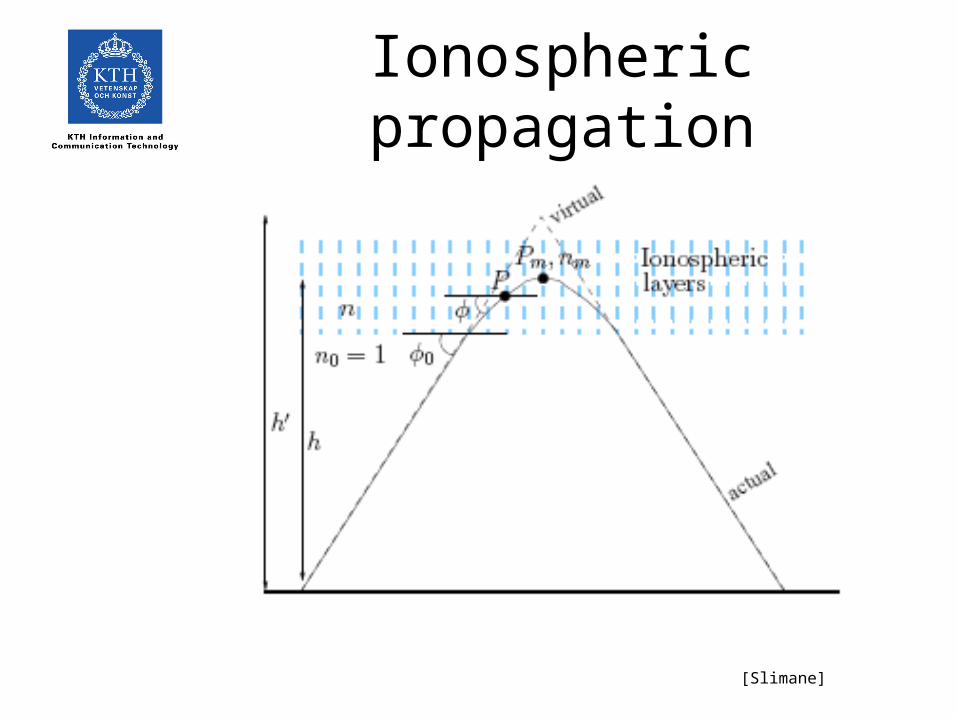
Refraction in an ionospheric layer
[Slimane]

Electron density profile
[Slimane]
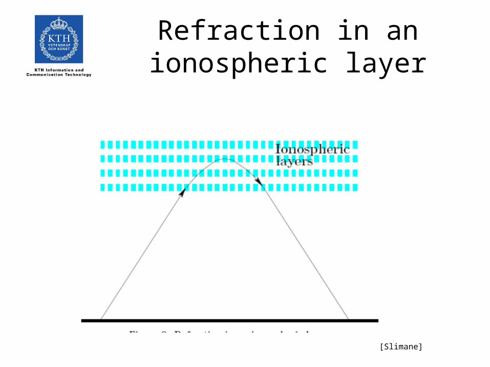
Ray paths
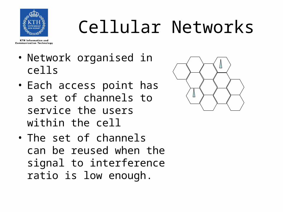
Cellular Networks
• Network organised in cells• Each access point has a set
of channels to service the users within the cell
• The set of channels can be reused when the signal to interference ratio is low enough.
Macrocells
• Give services in urban, suburban and rural areas. The cell radii varies from about 1 km to many tens of km.
• Few users per area unit.
• Base stations antennas are mounted on high buildings or on masts to get better coverage.
Microcells
• In urban or suburban areas• Cell radii is approximately 500 m• Very high traffic density (many users per
area unit).• Antennas mounted lower than the
buildings around it to decrease the cell coverage are
• More cells/unit area can services more users.
Indoor Cells (Picocells)
• High data rates and high traffic densities for both mobile and fixed users
• Coverage area influenced by– Layout of the building– Construction material (wood transparent to
radio waves, well reinforced concrete is not).– Shape of rooms
Propagation modelling
• To predict coverage areas in mobile cellular telephone systems, simple propagation models are needed.– Empirical methods– Physical models– Hybrid methods
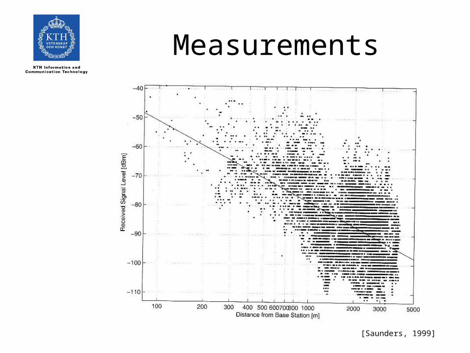
Measurements
[Saunders, 1999]
Emperical methods
• Models are usually based on actual path loss measurements.– Curve fitting is used to obtain an analytical function for
the model.– Parameters are given by: distance, frequency,
antenna heights, distance to nearest building.
• Validity of the model may be limited (dependent on the environment)
• Models are practical and easy to use but not very accurate.

Physical Models
• A physical model needs a very detailed description of the terrain and other clutter.– Large amount of data needed.– Excessive computational effort needed.
• The important parameter for the macrocell designer is the area covered, not the field strength at particular locations.
Computerised Planning Tools
• The enormous increase in the need to plan cellular systems accurately and quickly
• The development of fast, affordable computing resources
• The development of geographical information systems
• Example:– TEMS CellPlanner, Ericsson AB
Empircal Models for Macro Cells
• Power Law models
• Clutter factor models
• Okumura-Hata model
• Cost 231-Hata Model

Plane Earth Loss
[Saunders, 1999]
Physical Models for Macro Cells
• Ikegami Model
• Rooftop diffraction
• Flat Edge model
• Walfisch-Bertoni model
• COST 231/Walfisch-Ikegami model
Models for Micro Cells
• Dual Slope model (empirical model)
• Physical Models– Two-ray model– Street canyon models– Non-line-of-sight models

Picocells
• Wall and floor factor models
• COST231 Multi-wall model
• Ericsson model
• COST 231 Line-of-sight model
• Floor Gain Models
• COST 231 Non-Line-of Sight model
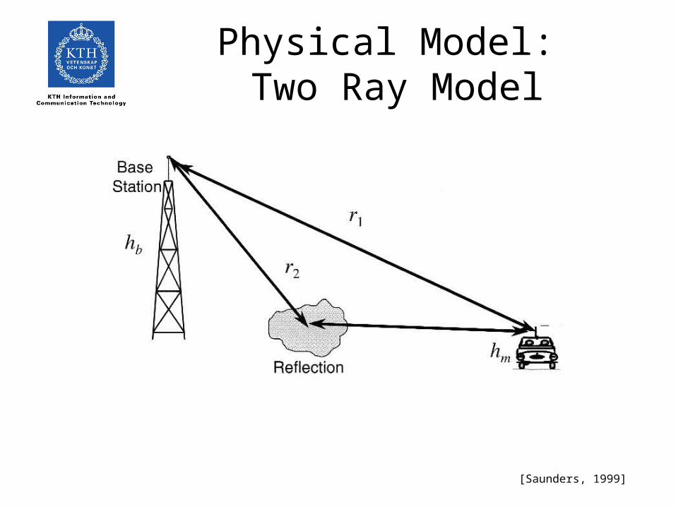
Physical Model: Two Ray Model
[Saunders, 1999]
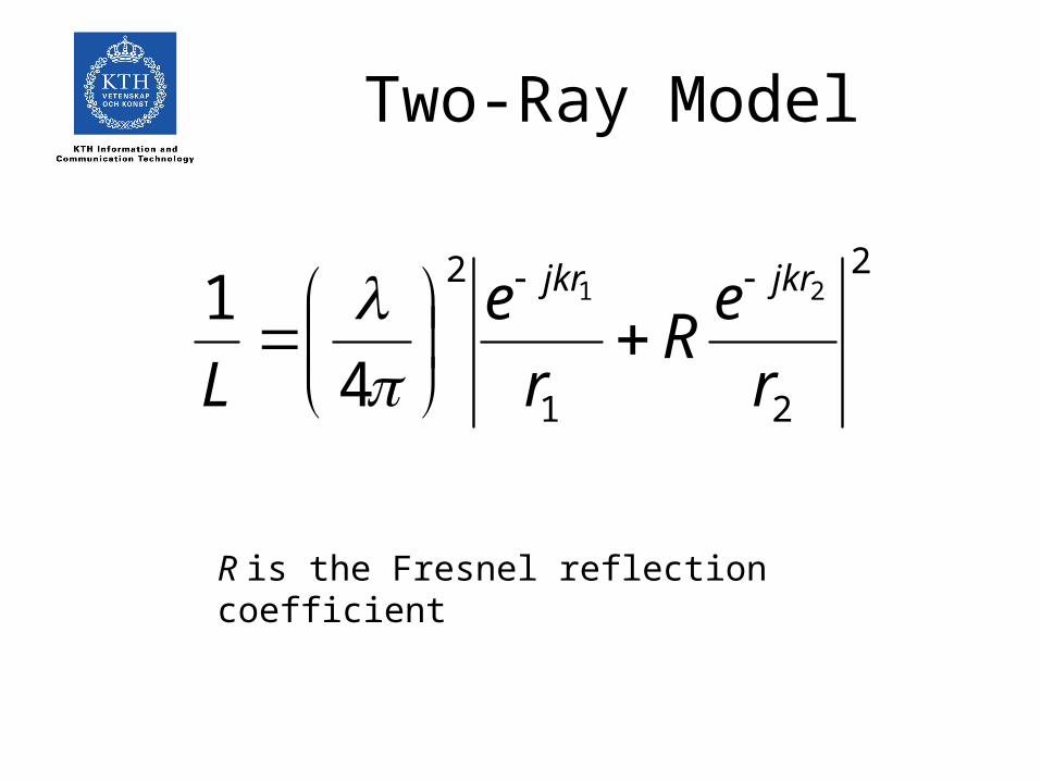
Two-Ray Model
2
21
221
4
1
r
eR
r
e
L
jkrjkr
R is the Fresnel reflection coefficient
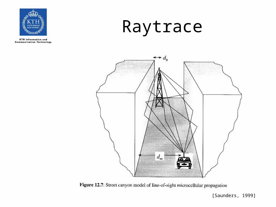
Raytrace
[Saunders, 1999]

Indoor models