Embed Size (px)
Citation preview

Lecture 3: Model-Free Policy Evaluation: PolicyEvaluation Without Knowing How the World Works1
Emma Brunskill
CS234 Reinforcement Learning
Winter 2020
1Material builds on structure from David SIlver’s Lecture 4: Model-Free Prediction.Other resources: Sutton and Barto Jan 1 2018 draft Chapter/Sections: 5.1; 5.5; 6.1-6.3
Emma Brunskill (CS234 Reinforcement Learning)Lecture 3: Model-Free Policy Evaluation: Policy Evaluation Without Knowing How the World Works1Winter 2020 1 / 56

Refresh Your Knowledge 2 [Piazza Poll]
What is the max number of iterations of policy iteration in a tabular MDP?
1 |A||S |2 |S ||A|3 |A||S|4 Unbounded5 Not sure
In a tabular MDP asymptotically value iteration will always yield a policywith the same value as the policy returned by policy iteration
1 True.2 False3 Not sure
Can value iteration require more iterations than |A||S| to compute theoptimal value function? (Assume |A| and |S | are small enough that eachround of value iteration can be done exactly).
1 True.2 False3 Not sure
Emma Brunskill (CS234 Reinforcement Learning)Lecture 3: Model-Free Policy Evaluation: Policy Evaluation Without Knowing How the World Works1Winter 2020 2 / 56

Refresh Your Knowledge 2
What is the max number of iterations of policy iteration in a tabular MDP?
Can value iteration require more iterations than |A||S| to compute theoptimal value function? (Assume |A| and |S | are small enough that eachround of value iteration can be done exactly).
In a tabular MDP asymptotically value iteration will always yield a policywith the same value as the policy returned by policy iteration
Emma Brunskill (CS234 Reinforcement Learning)Lecture 3: Model-Free Policy Evaluation: Policy Evaluation Without Knowing How the World Works1Winter 2020 3 / 56

Today’s Plan
Last Time:
Markov reward / decision processesPolicy evaluation & control when have true model (of how the world works)
Today
Policy evaluation without known dynamics & reward models
Next Time:
Control when don’t have a model of how the world works
Emma Brunskill (CS234 Reinforcement Learning)Lecture 3: Model-Free Policy Evaluation: Policy Evaluation Without Knowing How the World Works1Winter 2020 4 / 56

This Lecture: Policy Evaluation
Estimating the expected return of a particular policy if don’t have access totrue MDP models
Dynamic programming
Monte Carlo policy evaluation
Policy evaluation when don’t have a model of how the world work
Given on-policy samples
Temporal Difference (TD)
Metrics to evaluate and compare algorithms
Emma Brunskill (CS234 Reinforcement Learning)Lecture 3: Model-Free Policy Evaluation: Policy Evaluation Without Knowing How the World Works1Winter 2020 5 / 56

Recall
Definition of Return, Gt (for a MRP)
Discounted sum of rewards from time step t to horizon
Gt = rt + γrt+1 + γ2rt+2 + γ3rt+3 + · · ·
Definition of State Value Function, V π(s)
Expected return from starting in state s under policy π
V π(s) = Eπ[Gt |st = s] = Eπ[rt + γrt+1 + γ2rt+2 + γ3rt+3 + · · · |st = s]
Definition of State-Action Value Function, Qπ(s, a)
Expected return from starting in state s, taking action a and then followingpolicy π
Qπ(s, a) = Eπ[Gt |st = s, at = a]
= Eπ[rt + γrt+1 + γ2rt+2 + γ3rt+3 + · · · |st = s, at = a]
Emma Brunskill (CS234 Reinforcement Learning)Lecture 3: Model-Free Policy Evaluation: Policy Evaluation Without Knowing How the World Works1Winter 2020 6 / 56
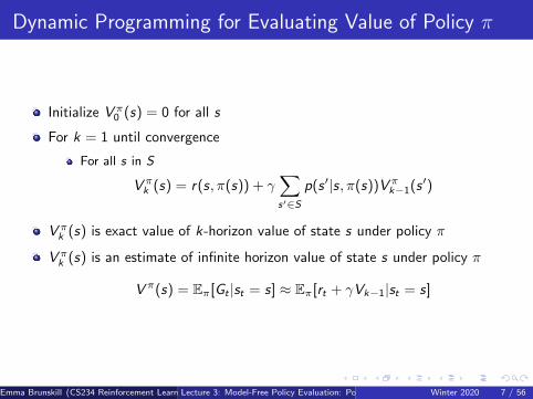
Dynamic Programming for Evaluating Value of Policy π
Initialize V π0 (s) = 0 for all s
For k = 1 until convergence
For all s in S
V πk (s) = r(s, π(s)) + γ
∑s′∈S
p(s ′|s, π(s))V πk−1(s ′)
V πk (s) is exact value of k-horizon value of state s under policy π
V πk (s) is an estimate of infinite horizon value of state s under policy π
V π(s) = Eπ[Gt |st = s] ≈ Eπ[rt + γVk−1|st = s]
Emma Brunskill (CS234 Reinforcement Learning)Lecture 3: Model-Free Policy Evaluation: Policy Evaluation Without Knowing How the World Works1Winter 2020 7 / 56

Dynamic Programming Policy EvaluationV π(s)← Eπ[rt + γVk−1|st = s]
Emma Brunskill (CS234 Reinforcement Learning)Lecture 3: Model-Free Policy Evaluation: Policy Evaluation Without Knowing How the World Works1Winter 2020 8 / 56

Dynamic Programming Policy EvaluationV π(s)← Eπ[rt + γVk−1|st = s]
Emma Brunskill (CS234 Reinforcement Learning)Lecture 3: Model-Free Policy Evaluation: Policy Evaluation Without Knowing How the World Works1Winter 2020 9 / 56

Dynamic Programming Policy EvaluationV π(s)← Eπ[rt + γVk−1|st = s]
Emma Brunskill (CS234 Reinforcement Learning)Lecture 3: Model-Free Policy Evaluation: Policy Evaluation Without Knowing How the World Works1Winter 2020 10 / 56

Dynamic Programming Policy EvaluationV π(s)← Eπ[rt + γVk−1|st = s]
Emma Brunskill (CS234 Reinforcement Learning)Lecture 3: Model-Free Policy Evaluation: Policy Evaluation Without Knowing How the World Works1Winter 2020 11 / 56
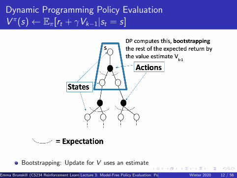
Dynamic Programming Policy EvaluationV π(s)← Eπ[rt + γVk−1|st = s]
Bootstrapping: Update for V uses an estimate
Emma Brunskill (CS234 Reinforcement Learning)Lecture 3: Model-Free Policy Evaluation: Policy Evaluation Without Knowing How the World Works1Winter 2020 12 / 56
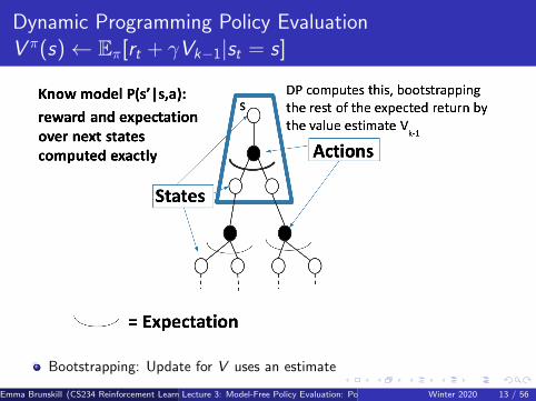
Dynamic Programming Policy EvaluationV π(s)← Eπ[rt + γVk−1|st = s]
Bootstrapping: Update for V uses an estimate
Emma Brunskill (CS234 Reinforcement Learning)Lecture 3: Model-Free Policy Evaluation: Policy Evaluation Without Knowing How the World Works1Winter 2020 13 / 56

Policy Evaluation: V π(s) = Eπ[Gt |st = s]
Gt = rt + γrt+1 + γ2rt+2 + γ3rt+3 + · · · in MDP M under policy π
Dynamic Programming
V π(s) ≈ Eπ[rt + γVk−1|st = s]Requires model of MDP MBootstraps future return using value estimateRequires Markov assumption: bootstrapping regardless of history
What if don’t know dynamics model P and/ or reward model R?
Today: Policy evaluation without a model
Given data and/or ability to interact in the environmentEfficiently compute a good estimate of a policy π
For example: Estimate expected total purchases during an online shoppingsession for a new automated product recommendation policy
Emma Brunskill (CS234 Reinforcement Learning)Lecture 3: Model-Free Policy Evaluation: Policy Evaluation Without Knowing How the World Works1Winter 2020 14 / 56

This Lecture Overview: Policy Evaluation
Dynamic Programming
Evaluating the quality of an estimator
Monte Carlo policy evaluation
Policy evaluation when don’t know dynamics and/or reward model
Given on policy samples
Temporal Difference (TD)
Metrics to evaluate and compare algorithms
Emma Brunskill (CS234 Reinforcement Learning)Lecture 3: Model-Free Policy Evaluation: Policy Evaluation Without Knowing How the World Works1Winter 2020 15 / 56

Monte Carlo (MC) Policy Evaluation
Gt = rt + γrt+1 + γ2rt+2 + γ3rt+3 + · · · in MDP M under policy π
V π(s) = ET∼π[Gt |st = s]
Expectation over trajectories T generated by following π
Simple idea: Value = mean return
If trajectories are all finite, sample set of trajectories & average returns
Emma Brunskill (CS234 Reinforcement Learning)Lecture 3: Model-Free Policy Evaluation: Policy Evaluation Without Knowing How the World Works1Winter 2020 16 / 56

Monte Carlo (MC) Policy Evaluation
If trajectories are all finite, sample set of trajectories & average returns
Does not require MDP dynamics/rewards
No bootstrapping
Does not assume state is Markov
Can only be applied to episodic MDPs
Averaging over returns from a complete episodeRequires each episode to terminate
Emma Brunskill (CS234 Reinforcement Learning)Lecture 3: Model-Free Policy Evaluation: Policy Evaluation Without Knowing How the World Works1Winter 2020 17 / 56

Monte Carlo (MC) On Policy Evaluation
Aim: estimate V π(s) given episodes generated under policy π
s1, a1, r1, s2, a2, r2, . . . where the actions are sampled from π
Gt = rt + γrt+1 + γ2rt+2 + γ3rt+3 + · · · in MDP M under policy π
V π(s) = Eπ[Gt |st = s]
MC computes empirical mean return
Often do this in an incremental fashion
After each episode, update estimate of V π
Emma Brunskill (CS234 Reinforcement Learning)Lecture 3: Model-Free Policy Evaluation: Policy Evaluation Without Knowing How the World Works1Winter 2020 18 / 56

First-Visit Monte Carlo (MC) On Policy Evaluation
Initialize N(s) = 0, G (s) = 0 ∀s ∈ SLoop
Sample episode i = si,1, ai,1, ri,1, si,2, ai,2, ri,2, . . . , si,Ti
Define Gi,t = ri,t + γri,t+1 + γ2ri,t+2 + · · · γTi−1ri,Ti as return from timestep t onwards in ith episode
For each state s visited in episode i
For first time t that state s is visited in episode i
Increment counter of total first visits: N(s) = N(s) + 1Increment total return G(s) = G(s) + Gi,t
Update estimate V π(s) = G(s)/N(s)
Emma Brunskill (CS234 Reinforcement Learning)Lecture 3: Model-Free Policy Evaluation: Policy Evaluation Without Knowing How the World Works1Winter 2020 19 / 56

Bias, Variance and MSE
Consider a statistical model that is parameterized by θ and that determinesa probability distribution over observed data P(x |θ)
Consider a statistic θ̂ that provides an estimate of θ and is a function ofobserved data x
E.g. for a Gaussian distribution with known variance, the average of a set ofi.i.d data points is an estimate of the mean of the Gaussian
Definition: the bias of an estimator θ̂ is:
Biasθ(θ̂) = Ex|θ[θ̂]− θ
Definition: the variance of an estimator θ̂ is:
Var(θ̂) = Ex|θ[(θ̂ − E[θ̂])2]
Definition: mean squared error (MSE) of an estimator θ̂ is:
MSE (θ̂) = Var(θ̂) + Biasθ(θ̂)2
Emma Brunskill (CS234 Reinforcement Learning)Lecture 3: Model-Free Policy Evaluation: Policy Evaluation Without Knowing How the World Works1Winter 2020 20 / 56

First-Visit Monte Carlo (MC) On Policy Evaluation
Initialize N(s) = 0, G (s) = 0 ∀s ∈ SLoop
Sample episode i = si,1, ai,1, ri,1, si,2, ai,2, ri,2, . . . , si,Ti
Define Gi,t = ri,t + γri,t+1 + γ2ri,t+2 + · · · γTi−1ri,Ti as return from timestep t onwards in ith episode
For each state s visited in episode i
For first time t that state s is visited in episode i
Increment counter of total first visits: N(s) = N(s) + 1Increment total return G(s) = G(s) + Gi,t
Update estimate V π(s) = G(s)/N(s)
Properties:
V π estimator is an unbiased estimator of true Eπ[Gt |st = s]
By law of large numbers, as N(s)→∞, V π(s)→ Eπ[Gt |st = s]
Emma Brunskill (CS234 Reinforcement Learning)Lecture 3: Model-Free Policy Evaluation: Policy Evaluation Without Knowing How the World Works1Winter 2020 21 / 56

Every-Visit Monte Carlo (MC) On Policy Evaluation
Initialize N(s) = 0, G (s) = 0 ∀s ∈ SLoop
Sample episode i = si,1, ai,1, ri,1, si,2, ai,2, ri,2, . . . , si,Ti
Define Gi,t = ri,t + γri,t+1 + γ2ri,t+2 + · · · γTi−1ri,Ti as return from timestep t onwards in ith episode
For each state s visited in episode i
For every time t that state s is visited in episode i
Increment counter of total first visits: N(s) = N(s) + 1Increment total return G(s) = G(s) + Gi,t
Update estimate V π(s) = G(s)/N(s)
Emma Brunskill (CS234 Reinforcement Learning)Lecture 3: Model-Free Policy Evaluation: Policy Evaluation Without Knowing How the World Works1Winter 2020 22 / 56

Every-Visit Monte Carlo (MC) On Policy Evaluation
Initialize N(s) = 0, G (s) = 0 ∀s ∈ SLoop
Sample episode i = si,1, ai,1, ri,1, si,2, ai,2, ri,2, . . . , si,Ti
Define Gi,t = ri,t + γri,t+1 + γ2ri,t+2 + · · · γTi−1ri,Ti as return from timestep t onwards in ith episode
For each state s visited in episode i
For every time t that state s is visited in episode i
Increment counter of total first visits: N(s) = N(s) + 1Increment total return G(s) = G(s) + Gi,t
Update estimate V π(s) = G(s)/N(s)
Properties:
V π every-visit MC estimator is a biased estimator of V π
But consistent estimator and often has better MSE
Emma Brunskill (CS234 Reinforcement Learning)Lecture 3: Model-Free Policy Evaluation: Policy Evaluation Without Knowing How the World Works1Winter 2020 23 / 56

Worked Example First Visit MC On Policy Evaluation
Initialize N(s) = 0, G(s) = 0 ∀s ∈ S
Loop
Sample episode i = si,1, ai,1, ri,1, si,2, ai,2, ri,2, . . . , si,Ti
Gi,t = ri,t + γri,t+1 + γ2ri,t+2 + · · · γTi−1ri,Ti
For each state s visited in episode i
For first time t that state s is visited in episode iN(s) = N(s) + 1, G(s) = G(s) + Gi,t
Update estimate V π(s) = G(s)/N(s)
Mars rover: R = [ 1 0 0 0 0 0 +10] for any action
π(s) = a1 ∀s, γ = 1. any action from s1 and s7 terminates episode
Trajectory = (s3, a1, 0, s2, a1, 0, s2, a1, 0, s1, a1, 1, terminal)
Emma Brunskill (CS234 Reinforcement Learning)Lecture 3: Model-Free Policy Evaluation: Policy Evaluation Without Knowing How the World Works1Winter 2020 24 / 56

Worked Example MC On Policy Evaluation
Initialize N(s) = 0, G(s) = 0 ∀s ∈ S
Loop
Sample episode i = si,1, ai,1, ri,1, si,2, ai,2, ri,2, . . . , si,Ti
Gi,t = ri,t + γri,t+1 + γ2ri,t+2 + · · · γTi−1ri,Ti
For each state s visited in episode i
For first or every time t that state s is visited in episode iN(s) = N(s) + 1, G(s) = G(s) + Gi,t
Update estimate V π(s) = G(s)/N(s)
Mars rover: R = [ 1 0 0 0 0 0 +10] for any action
Trajectory = (s3, a1, 0, s2, a1, 0, s2, a1, 0, s1, a1, 1, terminal)
Let γ = 1. First visit MC estimate of V of each state?
Now let γ = 0.9. Compare the first visit & every visit MC estimates of s2.
Emma Brunskill (CS234 Reinforcement Learning)Lecture 3: Model-Free Policy Evaluation: Policy Evaluation Without Knowing How the World Works1Winter 2020 25 / 56

Incremental Monte Carlo (MC) On Policy Evaluation
After each episode i = si ,1, ai ,1, ri ,1, si ,2, ai ,2, ri ,2, . . .
Define Gi,t = ri,t + γri,t+1 + γ2ri,t+2 + · · · as return from time step tonwards in ith episode
For state s visited at time step t in episode i
Increment counter of total first visits: N(s) = N(s) + 1Update estimate
V π(s) = V π(s)N(s)− 1
N(s)+
Gi ,t
N(s)= V π(s) +
1
N(s)(Gi ,t − V π(s))
Emma Brunskill (CS234 Reinforcement Learning)Lecture 3: Model-Free Policy Evaluation: Policy Evaluation Without Knowing How the World Works1Winter 2020 26 / 56

Check Your Understanding: Piazza Poll Incremental MC
First or Every Visit MC
Sample episode i = si,1, ai,1, ri,1, si,2, ai,2, ri,2, . . . , si,Ti
Gi,t = ri,t + γri,t+1 + γ2ri,t+2 + · · · γTi−1ri,Ti
For all s, for first or every time t that state s is visited in episode iN(s) = N(s) + 1, G(s) = G(s) + Gi,t
Update estimate V π(s) = G(s)/N(s)
Incremental MC
Sample episode i = si,1, ai,1, ri,1, si,2, ai,2, ri,2, . . . , si,Ti
Gi,t = ri,t + γri,t+1 + γ2ri,t+2 + · · · γTi−1ri,Ti
for i = 1 : H
V π(si ) = V π(si ) + α(Gi,t − V π(si ))
1 Incremental MC with α = 1 is the same as first visit MC
2 Incremental MC with α = 1N(s) is the same as first visit MC
3 Incremental MC with α = 1N(s) is the same as every visit MC
4 Incremental MC with α > 1N(s) could be helpful in non-stationary domains
Emma Brunskill (CS234 Reinforcement Learning)Lecture 3: Model-Free Policy Evaluation: Policy Evaluation Without Knowing How the World Works1Winter 2020 27 / 56

Check Your Understanding: Piazza Poll Incremental MC
First or Every Visit MC
Sample episode i = si,1, ai,1, ri,1, si,2, ai,2, ri,2, . . . , si,Ti
Gi,t = ri,t + γri,t+1 + γ2ri,t+2 + · · · γTi−1ri,Ti
For all s, for first or every time t that state s is visited in episode i
N(s) = N(s) + 1, G(s) = G(s) + Gi,t
Update estimate V π(s) = G(s)/N(s)
Incremental MC
Sample episode i = si,1, ai,1, ri,1, si,2, ai,2, ri,2, . . . , si,Ti
Gi,t = ri,t + γri,t+1 + γ2ri,t+2 + · · · γTi−1ri,Ti
for i = 1 : H
V π(si ) = V π(si ) + α(Gi,t − V π(si ))
Emma Brunskill (CS234 Reinforcement Learning)Lecture 3: Model-Free Policy Evaluation: Policy Evaluation Without Knowing How the World Works1Winter 2020 28 / 56

MC Policy Evaluation
V π(s) = V π(s) + α(Gi ,t − V π(s))
Emma Brunskill (CS234 Reinforcement Learning)Lecture 3: Model-Free Policy Evaluation: Policy Evaluation Without Knowing How the World Works1Winter 2020 29 / 56

MC Policy Evaluation
V π(s) = V π(s) + α(Gi ,t − V π(s))
Emma Brunskill (CS234 Reinforcement Learning)Lecture 3: Model-Free Policy Evaluation: Policy Evaluation Without Knowing How the World Works1Winter 2020 30 / 56

Monte Carlo (MC) Policy Evaluation Key Limitations
Generally high variance estimator
Reducing variance can require a lot of dataIn cases where data is very hard or expensive to acquire, or the stakes arehigh, MC may be impractical
Requires episodic settings
Episode must end before data from episode can be used to update V
Emma Brunskill (CS234 Reinforcement Learning)Lecture 3: Model-Free Policy Evaluation: Policy Evaluation Without Knowing How the World Works1Winter 2020 31 / 56

Monte Carlo (MC) Policy Evaluation Summary
Aim: estimate V π(s) given episodes generated under policy π
s1, a1, r1, s2, a2, r2, . . . where the actions are sampled from π
Gt = rt + γrt+1 + γ2rt+2 + γ3rt+3 + · · · under policy π
V π(s) = Eπ[Gt |st = s]
Simple: Estimates expectation by empirical average (given episodes sampledfrom policy of interest)
Updates V estimate using sample of return to approximate the expectation
No bootstrapping
Does not assume Markov process
Converges to true value under some (generally mild) assumptions
Emma Brunskill (CS234 Reinforcement Learning)Lecture 3: Model-Free Policy Evaluation: Policy Evaluation Without Knowing How the World Works1Winter 2020 32 / 56

This Lecture: Policy Evaluation
Estimating the expected return of a particular policy if don’t have access totrue MDP models
Dynamic programming
Monte Carlo policy evaluation
Policy evaluation when don’t have a model of how the world work
Given on-policy samples
Temporal Difference (TD)
Metrics to evaluate and compare algorithms
Emma Brunskill (CS234 Reinforcement Learning)Lecture 3: Model-Free Policy Evaluation: Policy Evaluation Without Knowing How the World Works1Winter 2020 33 / 56

Temporal Difference Learning
“If one had to identify one idea as central and novel to reinforcementlearning, it would undoubtedly be temporal-difference (TD) learning.” –Sutton and Barto 2017
Combination of Monte Carlo & dynamic programming methods
Model-free
Bootstraps and samples
Can be used in episodic or infinite-horizon non-episodic settings
Immediately updates estimate of V after each (s, a, r , s ′) tuple
Emma Brunskill (CS234 Reinforcement Learning)Lecture 3: Model-Free Policy Evaluation: Policy Evaluation Without Knowing How the World Works1Winter 2020 34 / 56

Temporal Difference Learning for Estimating V
Aim: estimate V π(s) given episodes generated under policy π
Gt = rt + γrt+1 + γ2rt+2 + γ3rt+3 + · · · in MDP M under policy π
V π(s) = Eπ[Gt |st = s]
Recall Bellman operator (if know MDP models)
BπV (s) = r(s, π(s)) + γ∑s′∈S
p(s ′|s, π(s))V (s ′)
In incremental every-visit MC, update estimate using 1 sample of return (forthe current ith episode)
V π(s) = V π(s) + α(Gi,t − V π(s))
Insight: have an estimate of V π, use to estimate expected return
V π(s) = V π(s) + α([rt + γV π(st+1)]− V π(s))
Emma Brunskill (CS234 Reinforcement Learning)Lecture 3: Model-Free Policy Evaluation: Policy Evaluation Without Knowing How the World Works1Winter 2020 35 / 56

Temporal Difference [TD(0)] Learning
Aim: estimate V π(s) given episodes generated under policy π
s1, a1, r1, s2, a2, r2, . . . where the actions are sampled from π
Simplest TD learning: update value towards estimated value
V π(st) = V π(st) + α([rt + γV π(st+1)]︸ ︷︷ ︸TD target
−V π(st))
TD error:δt = rt + γV π(st+1)− V π(st)
Can immediately update value estimate after (s, a, r , s ′) tuple
Don’t need episodic setting
Emma Brunskill (CS234 Reinforcement Learning)Lecture 3: Model-Free Policy Evaluation: Policy Evaluation Without Knowing How the World Works1Winter 2020 36 / 56

Temporal Difference [TD(0)] Learning Algorithm
Input: αInitialize V π(s) = 0, ∀s ∈ SLoop
Sample tuple (st , at , rt , st+1)
V π(st) = V π(st) + α([rt + γV π(st+1)]︸ ︷︷ ︸TD target
−V π(st))
Emma Brunskill (CS234 Reinforcement Learning)Lecture 3: Model-Free Policy Evaluation: Policy Evaluation Without Knowing How the World Works1Winter 2020 37 / 56

Worked Example TD Learning
Input: αInitialize V π(s) = 0, ∀s ∈ SLoop
Sample tuple (st , at , rt , st+1)
V π(st) = V π(st) + α([rt + γV π(st+1)]︸ ︷︷ ︸TD target
−V π(st))
Example:
Mars rover: R = [ 1 0 0 0 0 0 +10] for any action
π(s) = a1 ∀s, γ = 1. any action from s1 and s7 terminates episode
Trajectory = (s3, a1, 0, s2, a1, 0, s2, a1, 0, s1, a1, 1, terminal)
First visit MC estimate of V of each state? [1 1 1 0 0 0 0]
TD estimate of all states (init at 0) with α = 1?
Emma Brunskill (CS234 Reinforcement Learning)Lecture 3: Model-Free Policy Evaluation: Policy Evaluation Without Knowing How the World Works1Winter 2020 38 / 56

Check Your Understanding: Piazza Poll TemporalDifference [TD(0)] Learning Algorithm
Input: αInitialize V π(s) = 0, ∀s ∈ SLoop
Sample tuple (st , at , rt , st+1)
V π(st) = V π(st) + α([rt + γV π(st+1)]︸ ︷︷ ︸TD target
−V π(st))
Select all that are true
1 If α = 0 TD will value recent experience more
2 If α = 1 TD will value recent experience exclusively
3 If α = 1 TD in MDPs where the policy goes through states with multiplepossible next states, V may always oscillate
4 There exist deterministic MDPs where α = 1 TD will converge
Emma Brunskill (CS234 Reinforcement Learning)Lecture 3: Model-Free Policy Evaluation: Policy Evaluation Without Knowing How the World Works1Winter 2020 39 / 56

Check Your Understanding: Piazza Poll TemporalDifference [TD(0)] Learning Algorithm
Input: αInitialize V π(s) = 0, ∀s ∈ SLoop
Sample tuple (st , at , rt , st+1)
V π(st) = V π(st) + α([rt + γV π(st+1)]︸ ︷︷ ︸TD target
−V π(st))
Emma Brunskill (CS234 Reinforcement Learning)Lecture 3: Model-Free Policy Evaluation: Policy Evaluation Without Knowing How the World Works1Winter 2020 40 / 56

Temporal Difference Policy Evaluation
V π(st) = V π(st) + α([rt + γV π(st+1)]− V π(st))
Emma Brunskill (CS234 Reinforcement Learning)Lecture 3: Model-Free Policy Evaluation: Policy Evaluation Without Knowing How the World Works1Winter 2020 41 / 56
This Lecture: Policy Evaluation
Estimating the expected return of a particular policy if don’t have access totrue MDP models
Dynamic programming
Monte Carlo policy evaluation
Policy evaluation when don’t have a model of how the world work
Given on-policy samplesGiven off-policy samples
Temporal Difference (TD)
Metrics to evaluate and compare algorithms
Emma Brunskill (CS234 Reinforcement Learning)Lecture 3: Model-Free Policy Evaluation: Policy Evaluation Without Knowing How the World Works1Winter 2020 42 / 56

Check Your Understanding: Properties of Algorithms forEvaluation.
DP MC TD
Usable w/no models of domain
Handles continuing (non-episodic) setting
Assumes Markov process
Converges to true value in limit1
Unbiased estimate of value
DP = Dynamic Programming, MC = Monte Carlo, TD = TemporalDifference
1For tabular representations of value function. More on this in later lecturesEmma Brunskill (CS234 Reinforcement Learning)Lecture 3: Model-Free Policy Evaluation: Policy Evaluation Without Knowing How the World Works1Winter 2020 43 / 56

Some Important Properties to Evaluate Model-free PolicyEvaluation Algorithms
Bias/variance characteristics
Data efficiency
Computational efficiency
Emma Brunskill (CS234 Reinforcement Learning)Lecture 3: Model-Free Policy Evaluation: Policy Evaluation Without Knowing How the World Works1Winter 2020 44 / 56

Bias/Variance of Model-free Policy Evaluation Algorithms
Return Gt is an unbiased estimate of V π(st)
TD target [rt + γV π(st+1)] is a biased estimate of V π(st)
But often much lower variance than a single return Gt
Return function of multi-step sequence of random actions, states & rewards
TD target only has one random action, reward and next state
MC
Unbiased (for first visit)High varianceConsistent (converges to true) even with function approximation
TD
Some biasLower varianceTD(0) converges to true value with tabular representationTD(0) does not always converge with function approximation
Emma Brunskill (CS234 Reinforcement Learning)Lecture 3: Model-Free Policy Evaluation: Policy Evaluation Without Knowing How the World Works1Winter 2020 45 / 56

!" !# !$ !% !& !' !(
) !" = +1 ) !# = 0 ) !$ = 0 ) !% = 0 ) !& = 0 ) !' = 0 ) !( = +10./01/!123.2456 7214
89/:.2456 7214
Mars rover: R = [ 1 0 0 0 0 0 +10] for any action
π(s) = a1 ∀s, γ = 1. any action from s1 and s7 terminates episode
Trajectory = (s3, a1, 0, s2, a1, 0, s2, a1, 0, s1, a1, 1, terminal)
First visit MC estimate of V of each state? [1 1 1 0 0 0 0]
TD estimate of all states (init at 0) with α = 1 is [1 0 0 0 0 0 0]
TD(0) only uses a data point (s, a, r , s ′) once
Monte Carlo takes entire return from s to end of episode
Emma Brunskill (CS234 Reinforcement Learning)Lecture 3: Model-Free Policy Evaluation: Policy Evaluation Without Knowing How the World Works1Winter 2020 46 / 56

Batch MC and TD
Batch (Offline) solution for finite dataset
Given set of K episodesRepeatedly sample an episode from KApply MC or TD(0) to the sampled episode
What do MC and TD(0) converge to?
Emma Brunskill (CS234 Reinforcement Learning)Lecture 3: Model-Free Policy Evaluation: Policy Evaluation Without Knowing How the World Works1Winter 2020 47 / 56

AB Example: (Ex. 6.4, Sutton & Barto, 2018)
Two states A,B with γ = 1
Given 8 episodes of experience:
A, 0,B, 0B, 1 (observed 6 times)B, 0
Imagine run TD updates over data infinite number of times
V (B) = 0.75 by TD or MC (first visit or every visit)
Emma Brunskill (CS234 Reinforcement Learning)Lecture 3: Model-Free Policy Evaluation: Policy Evaluation Without Knowing How the World Works1Winter 2020 48 / 56

AB Example: (Ex. 6.4, Sutton & Barto, 2018)
TD Update: V π(st) = V π(st) + α([rt + γV π(st+1)]︸ ︷︷ ︸TD target
−V π(st))
Two states A,B with γ = 1
Given 8 episodes of experience:
A, 0,B, 0B, 1 (observed 6 times)B, 0
Imagine run TD updates over data infinite number of times
V (B) = 0.75 by TD or MC
What about V (A)?
Emma Brunskill (CS234 Reinforcement Learning)Lecture 3: Model-Free Policy Evaluation: Policy Evaluation Without Knowing How the World Works1Winter 2020 49 / 56

Batch MC and TD: Converges
Monte Carlo in batch setting converges to min MSE (mean squared error)
Minimize loss with respect to observed returnsIn AB example, V (A) = 0
TD(0) converges to DP policy V π for the MDP with the maximumlikelihood model estimates
Maximum likelihood Markov decision process model
P̂(s ′|s, a) =1
N(s, a)
K∑k=1
Lk−1∑t=1
1(sk,t = s, ak,t = a, sk,t+1 = s ′)
r̂(s, a) =1
N(s, a)
K∑k=1
Lk−1∑t=1
1(sk,t = s, ak,t = a)rt,k
Compute V π using this modelIn AB example, V (A) = 0.75
Emma Brunskill (CS234 Reinforcement Learning)Lecture 3: Model-Free Policy Evaluation: Policy Evaluation Without Knowing How the World Works1Winter 2020 50 / 56

Some Important Properties to Evaluate Model-free PolicyEvaluation Algorithms
Data efficiency & Computational efficiency
In simplest TD, use (s, a, r , s ′) once to update V (s)
O(1) operation per updateIn an episode of length L, O(L)
In MC have to wait till episode finishes, then also O(L)
MC can be more data efficient than simple TD
But TD exploits Markov structure
If in Markov domain, leveraging this is helpful
Emma Brunskill (CS234 Reinforcement Learning)Lecture 3: Model-Free Policy Evaluation: Policy Evaluation Without Knowing How the World Works1Winter 2020 51 / 56

Alternative: Certainty Equivalence V π MLE MDP ModelEstimates
Model-based option for policy evaluation without true models
After each (s, a, r , s ′) tuple
Recompute maximum likelihood MDP model for (s, a)
P̂(s ′|s, a) =1
N(s, a)
K∑k=1
Lk−1∑t=1
1(sk,t = s, ak,t = a, sk,t+1 = s ′)
r̂(s, a) =1
N(s, a)
K∑k=1
Lk−1∑t=1
1(sk,t = s, ak,t = a)rt,k
Compute V π using MLE MDP 2 (e.g. see method from lecture 2)
2Requires initializing for all (s, a) pairsEmma Brunskill (CS234 Reinforcement Learning)Lecture 3: Model-Free Policy Evaluation: Policy Evaluation Without Knowing How the World Works1Winter 2020 52 / 56

Alternative: Certainty Equivalence V π MLE MDP ModelEstimates
Model-based option for policy evaluation without true models
After each (s, a, r , s ′) tuple
Recompute maximum likelihood MDP model for (s, a)
P̂(s ′|s, a) =1
N(s, a)
K∑k=1
Lk−1∑t=1
1(sk,t = s, ak,t = a, sk,t+1 = s ′)
r̂(s, a) =1
N(s, a)
K∑k=1
Lk−1∑t=1
1(sk,t = s, ak,t = a)rt,k
Compute V π using MLE MDP
Cost: Updating MLE model and MDP planning at each update (O(|S |3) foranalytic matrix solution, O(|S |2|A|) for iterative methods)
Very data efficient and very computationally expensive
Consistent
Can also easily be used for off-policy evaluation
Emma Brunskill (CS234 Reinforcement Learning)Lecture 3: Model-Free Policy Evaluation: Policy Evaluation Without Knowing How the World Works1Winter 2020 53 / 56

!" !# !$ !% !& !' !(
) !" = +1 ) !# = 0 ) !$ = 0 ) !% = 0 ) !& = 0 ) !' = 0 ) !( = +10./01/!123.2456 7214
89/:.2456 7214
Mars rover: R = [ 1 0 0 0 0 0 +10] for any action
π(s) = a1 ∀s, γ = 1. any action from s1 and s7 terminates episode
Trajectory = (s3, a1, 0, s2, a1, 0, s2, a1, 0, s1, a1, 1, terminal)
First visit MC estimate of V of each state? [1 1 1 0 0 0 0]
Every visit MC estimate of V of s2? 1
TD estimate of all states (init at 0) with α = 1 is [1 0 0 0 0 0 0]
What is the certainty equivalent estimate?
Emma Brunskill (CS234 Reinforcement Learning)Lecture 3: Model-Free Policy Evaluation: Policy Evaluation Without Knowing How the World Works1Winter 2020 54 / 56
Summary: Policy Evaluation
Estimating the expected return of a particular policy if don’t have accessto true MDP models. Ex. evaluating average purchases per session of newproduct recommendation system
Dynamic Programming
Monte Carlo policy evaluation
Policy evaluation when we don’t have a model of how the world works
Given on policy samplesGiven off policy samples
Temporal Difference (TD)
Metrics to evaluate and compare algorithms
Robustness to Markov assumptionBias/variance characteristicsData efficiencyComputational efficiency
Emma Brunskill (CS234 Reinforcement Learning)Lecture 3: Model-Free Policy Evaluation: Policy Evaluation Without Knowing How the World Works1Winter 2020 55 / 56

Today’s Plan
Last Time:
Markov reward / decision processesPolicy evaluation & control when have true model (of how the world works)
Today
Policy evaluation without known dynamics & reward models
Next Time:
Control when don’t have a model of how the world works
Emma Brunskill (CS234 Reinforcement Learning)Lecture 3: Model-Free Policy Evaluation: Policy Evaluation Without Knowing How the World Works1Winter 2020 56 / 56