Embed Size (px)
Citation preview
Lecture 2.2 1 2015 Michael Stuart
Design and Analysis of ExperimentsLecture 2.2
1. Review Lecture 2.1
– Minute test– Why block?– Deleted residuals
2. Interaction
3. Random Block Effects
4. Introduction to 2-level factorial designs
– a 22 experiment– introducing the Design Matrix
Certificate in StatisticsDesign and Analysis of Experiments
Lecture 2.2 2 2015 Michael Stuart
How Much
5432
Certificate in StatisticsDesign and Analysis of Experiments
Lecture 2.2 3 2015 Michael Stuart
How Fast
4321
Certificate in StatisticsDesign and Analysis of Experiments
Lecture 2.2 4 2015 Michael Stuart
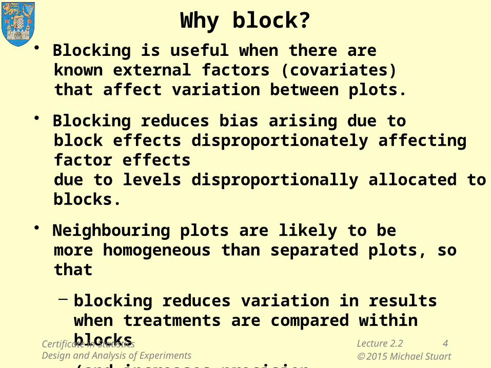
Why block?• Blocking is useful when there are
known external factors (covariates)that affect variation between plots.
• Blocking reduces bias arising due toblock effects disproportionately affecting factor effectsdue to levels disproportionally allocated to blocks.
• Neighbouring plots are likely to bemore homogeneous than separated plots, so that
– blocking reduces variation in resultswhen treatments are compared within blocks
– (and increases precisionwhen results are combined across blocks).
Certificate in StatisticsDesign and Analysis of Experiments
Lecture 2.2 5 2015 Michael Stuart
Deleted residuals
Minitab does this automatically for all cases!
They are used to allow each case to be assessed using a criterion not affected by the case.
The residuals are not deleted,
it is the case that is deleted
while the corresponding "deleted residual is calculated
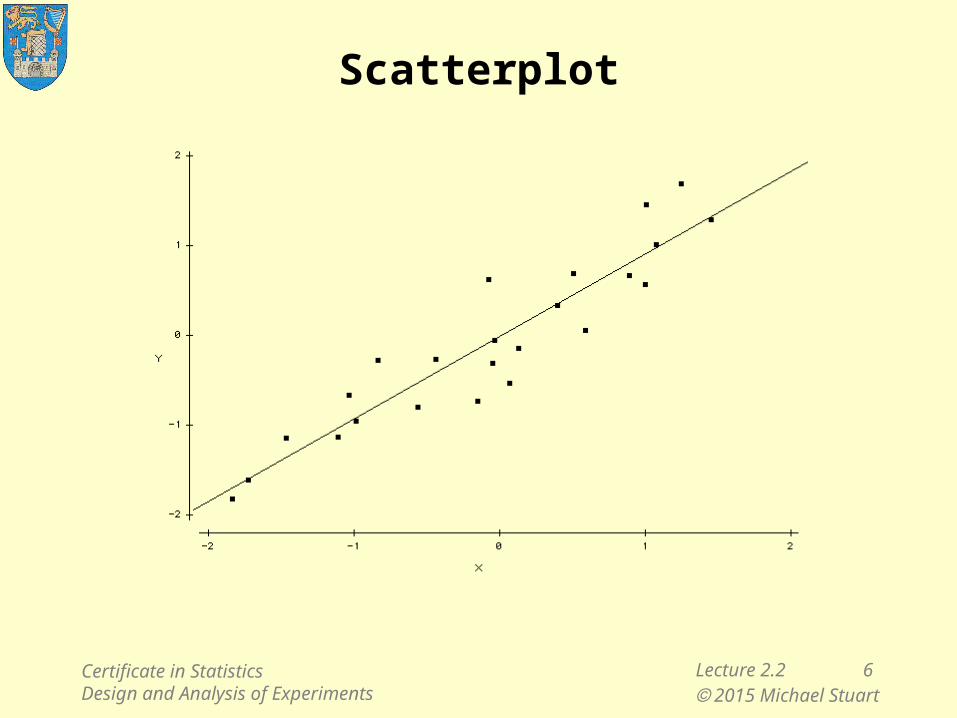
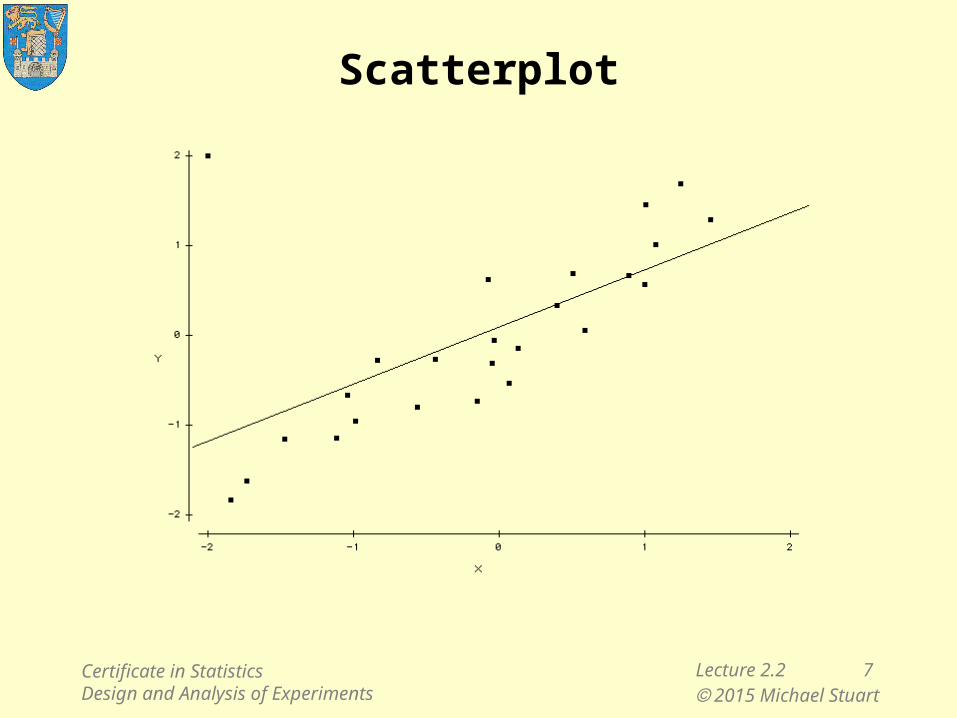
Simple linear regression illustrates:
Certificate in StatisticsDesign and Analysis of Experiments
Lecture 2.2 6 2015 Michael Stuart
Scatterplot
Certificate in StatisticsDesign and Analysis of Experiments
Lecture 2.2 7 2015 Michael Stuart
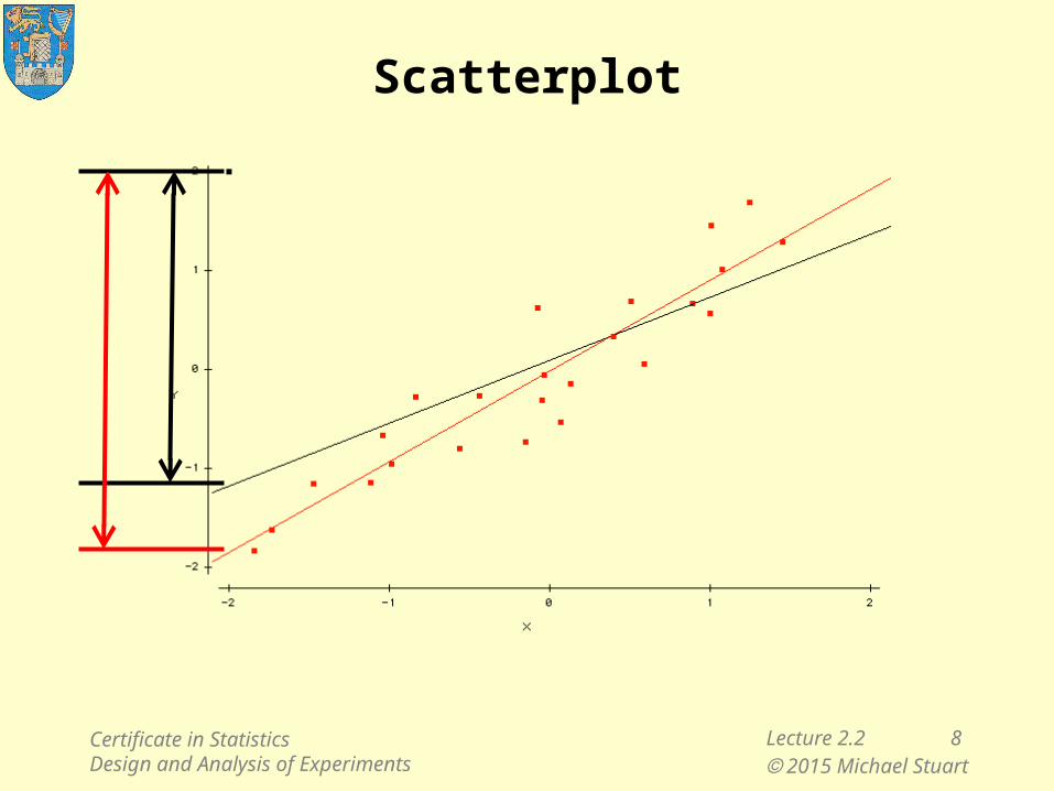
Scatterplot
Certificate in StatisticsDesign and Analysis of Experiments
Lecture 2.2 8 2015 Michael Stuart
Scatterplot
Certificate in StatisticsDesign and Analysis of Experiments
Lecture 2.2 9 2015 Michael Stuart
Deleted residual
Given an exceptional case,
deleted residual > residual using all the data
deleted s < s using all the data
deleted standardised residual
>> standardised residual using all the data
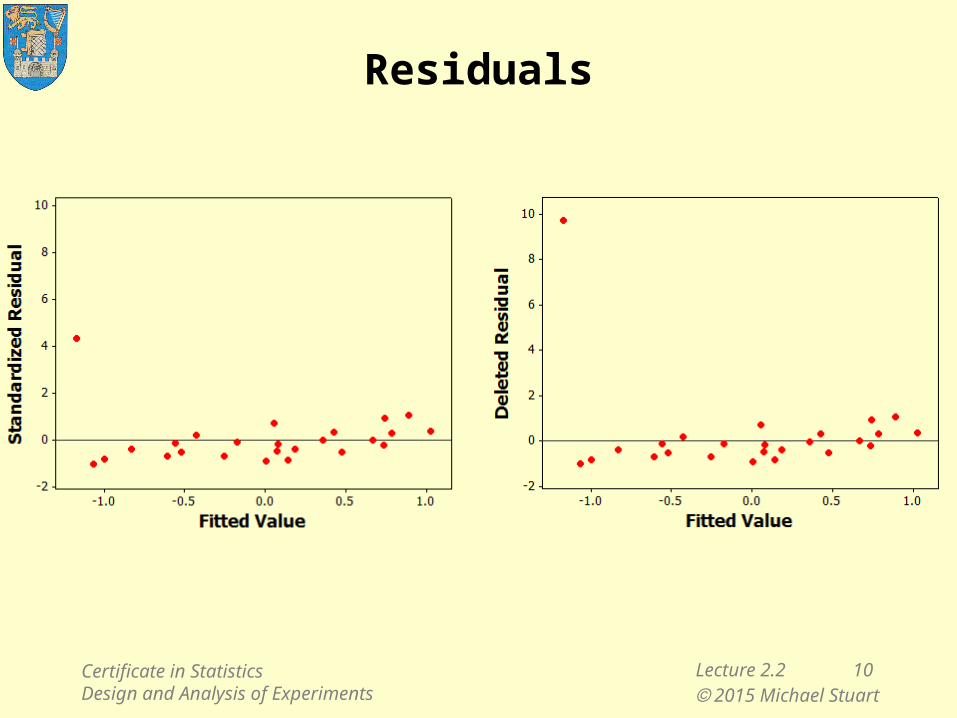
Using deleted residuals accentuates exceptional cases
Certificate in StatisticsDesign and Analysis of Experiments
Lecture 2.2 10 2015 Michael Stuart
Residuals
Certificate in StatisticsDesign and Analysis of Experiments
Lecture 2.2 11 2015 Michael Stuart
Design and Analysis of ExperimentsLecture 2.2
1. Review Lecture 2.1
– Minute test– Why block?– Deleted residuals
2. Interaction
3. Random Block Effects
4. Introduction to 2-level factorial designs
– a 22 experiment– introducing the Design Matrix
Certificate in StatisticsDesign and Analysis of Experiments
Lecture 2.2 12 2015 Michael Stuart
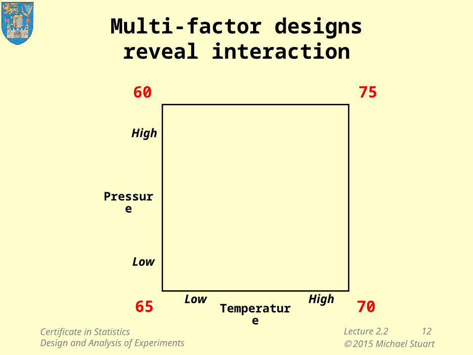
Multi-factor designsreveal interaction
Pressure
Temperature
High
High
Low
Low65
75
70
60
Certificate in StatisticsDesign and Analysis of Experiments
Lecture 2.2 13 2015 Michael Stuart
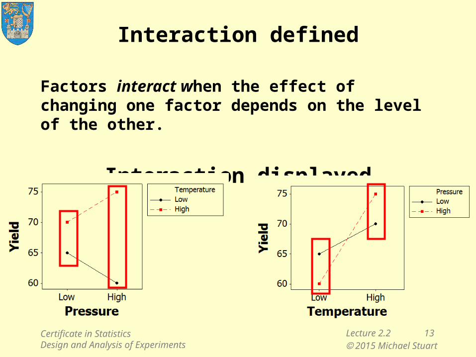
Interaction defined
Factors interact when the effect of changing one factor depends on the level of the other.
Interaction displayed
Certificate in StatisticsDesign and Analysis of Experiments
Lecture 2.2 14 2015 Michael Stuart
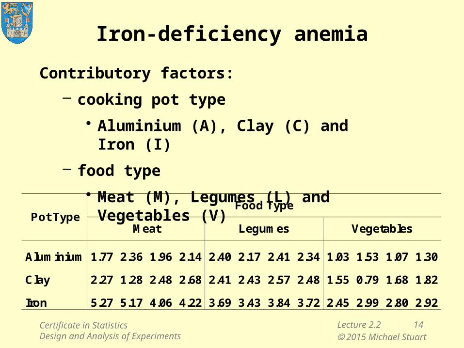
Iron-deficiency anemia
Contributory factors:
– cooking pot type
• Aluminium (A), Clay (C) and Iron (I)
– food type
• Meat (M), Legumes (L) and Vegetables (V)
Pot Type Food Type
Meat Legumes Vegetables
Aluminium 1.77 2.36 1.96 2.14 2.40 2.17 2.41 2.34 1.03 1.53 1.07 1.30
Clay 2.27 1.28 2.48 2.68 2.41 2.43 2.57 2.48 1.55 0.79 1.68 1.82
Iron 5.27 5.17 4.06 4.22 3.69 3.43 3.84 3.72 2.45 2.99 2.80 2.92
Certificate in StatisticsDesign and Analysis of Experiments
Lecture 2.2 15 2015 Michael Stuart
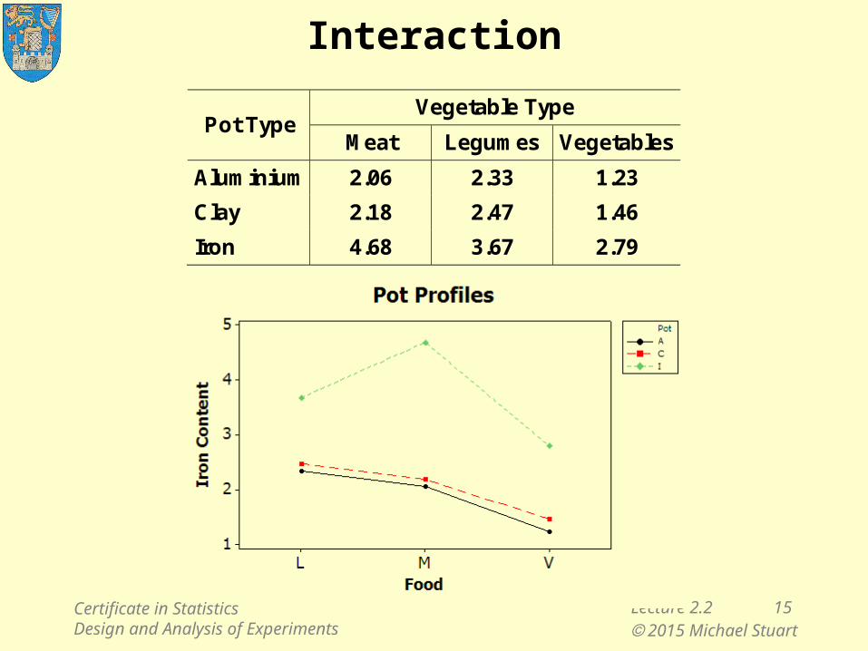
Interaction
Pot Type Vegetable Type
Meat Legumes Vegetables
Aluminium 2.06 2.33 1.23
Clay 2.18 2.47 1.46
Iron 4.68 3.67 2.79
Certificate in StatisticsDesign and Analysis of Experiments
Lecture 2.2 16 2015 Michael Stuart
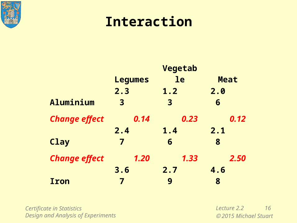
Interaction
Certificate in StatisticsDesign and Analysis of Experiments
Legumes Vegetable Meat
Aluminium 2.33 1.23 2.06
Change effect 0.14 0.23 0.12
Clay 2.47 1.46 2.18
Change effect 1.20 1.33 2.50
Iron 3.67 2.79 4.68
Lecture 2.2 17 2015 Michael Stuart
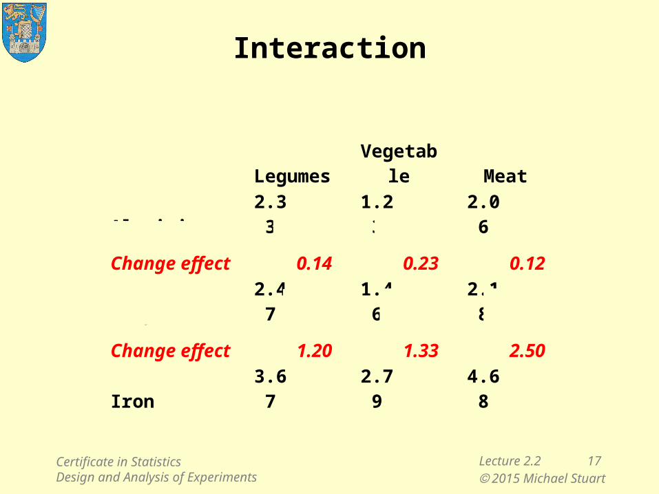
Interaction
Certificate in StatisticsDesign and Analysis of Experiments
Legumes Vegetable Meat
Aluminium 2.33 1.23 2.06
Change effect 0.14 0.23 0.12
Clay 2.47 1.46 2.18
Change effect 1.20 1.33 2.50
Iron 3.67 2.79 4.68

Lecture 2.2 18 2015 Michael Stuart
Two 2-level factors
Pressure
Temperature
High
High
Low
Low65
75
70
60 Pressure effect
Low T: 60 – 65 = –5High T: 75 – 70 = +5Diff: 5 – (–5) = 10
Temperature effect
Low P: 70 – 65 = 5High P: 75 – 60 = 15Diff: 15 – 5 = 10
Postgraduate Certificate in Statistics Design and Analysis of Experiments
Lecture 2.2 19 2015 Michael Stuart
Model for analysis
Iron content includes– a contribution for each food type
plus– a contribution for each pot type
plus– a contribution for each food type / pot type
combination
plus– a contribution due to chance variation
Certificate in StatisticsDesign and Analysis of Experiments
Lecture 2.2 20 2015 Michael Stuart
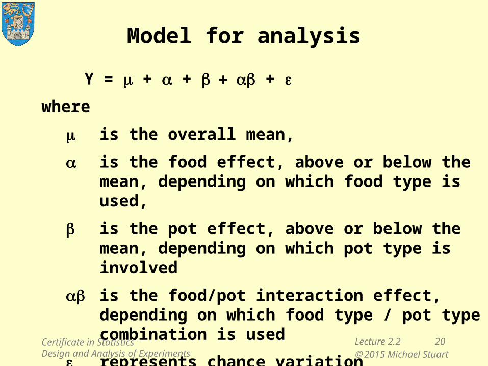
Model for analysis
Y = m + a + + b ab + e
where
m is the overall mean,
a is the food effect, above or below the mean, depending on which food type is used,
b is the pot effect, above or below the mean, depending on which pot type is involved
ab is the food/pot interaction effect, depending on which food type / pot type combination is used
e represents chance variation
Certificate in StatisticsDesign and Analysis of Experiments
Lecture 2.2 21 2015 Michael Stuart
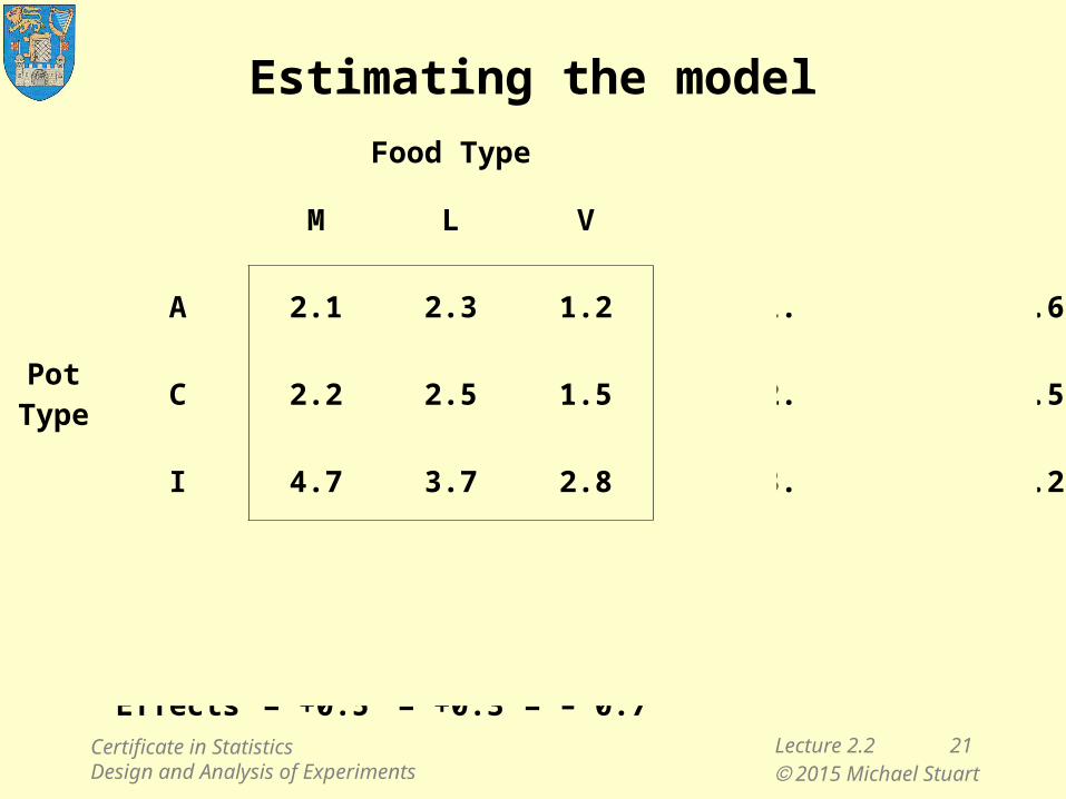
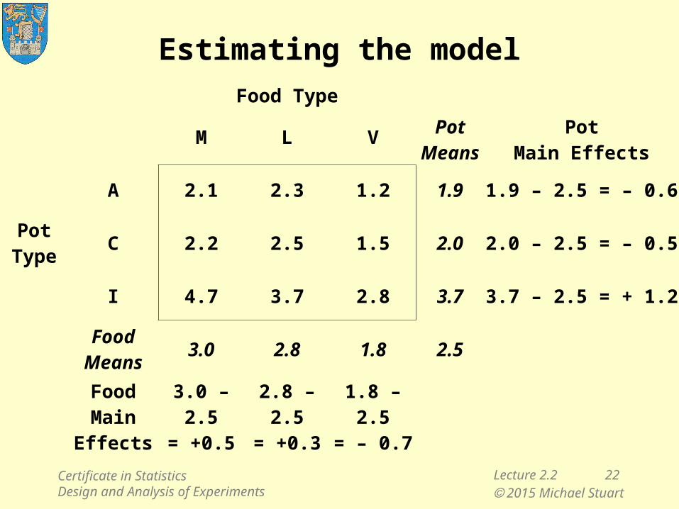
Estimating the model
Food Type
PotMeans
PotMain Effects
M L V
A 2.1 2.3 1.2 1.9 1.9 – 2.5 = – 0.6
PotType C 2.2 2.5 1.5 2.0 2.0 – 2.5 = – 0.5
I 4.7 3.7 2.8 3.7 3.7 – 2.5 = + 1.2
FoodMeans 3.0 2.8 1.8 2.5
FoodMain
Effects3.0 – 2.5= +0.5
2.8 – 2.5= +0.3
1.8 – 2.5= – 0.7
Certificate in StatisticsDesign and Analysis of Experiments
Lecture 2.2 22 2015 Michael Stuart
Estimating the model
Food Type
PotMeans
PotMain Effects
M L V
A 2.1 2.3 1.2 1.9 1.9 – 2.5 = – 0.6
PotType C 2.2 2.5 1.5 2.0 2.0 – 2.5 = – 0.5
I 4.7 3.7 2.8 3.7 3.7 – 2.5 = + 1.2
FoodMeans 3.0 2.8 1.8 2.5
FoodMain
Effects3.0 – 2.5= +0.5
2.8 – 2.5= +0.3
1.8 – 2.5= – 0.7
Certificate in StatisticsDesign and Analysis of Experiments
Lecture 2.2 23 2015 Michael Stuart
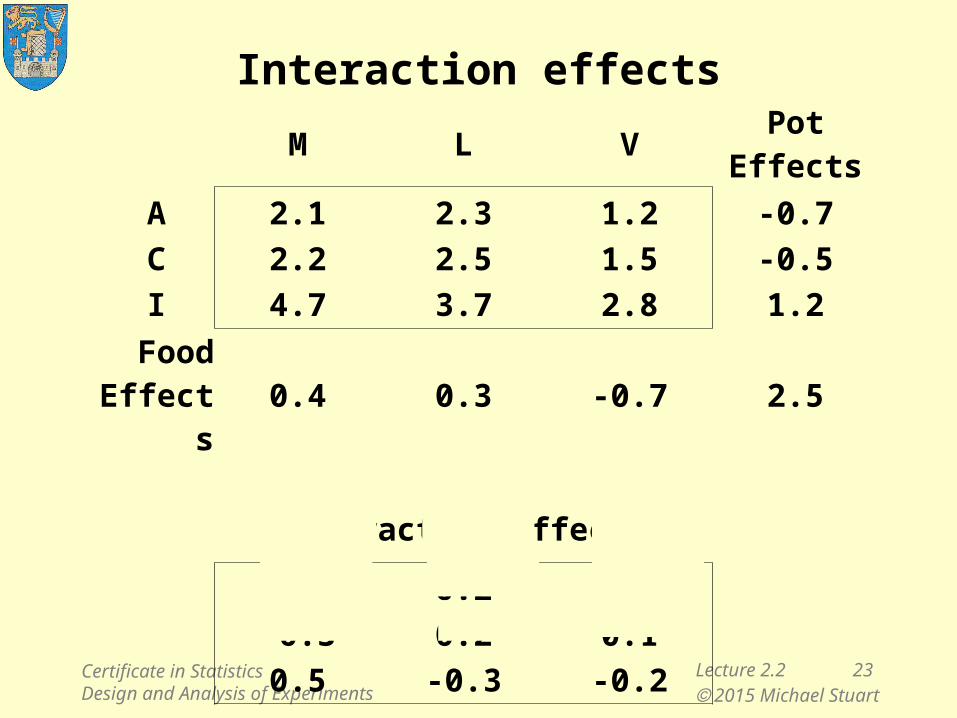
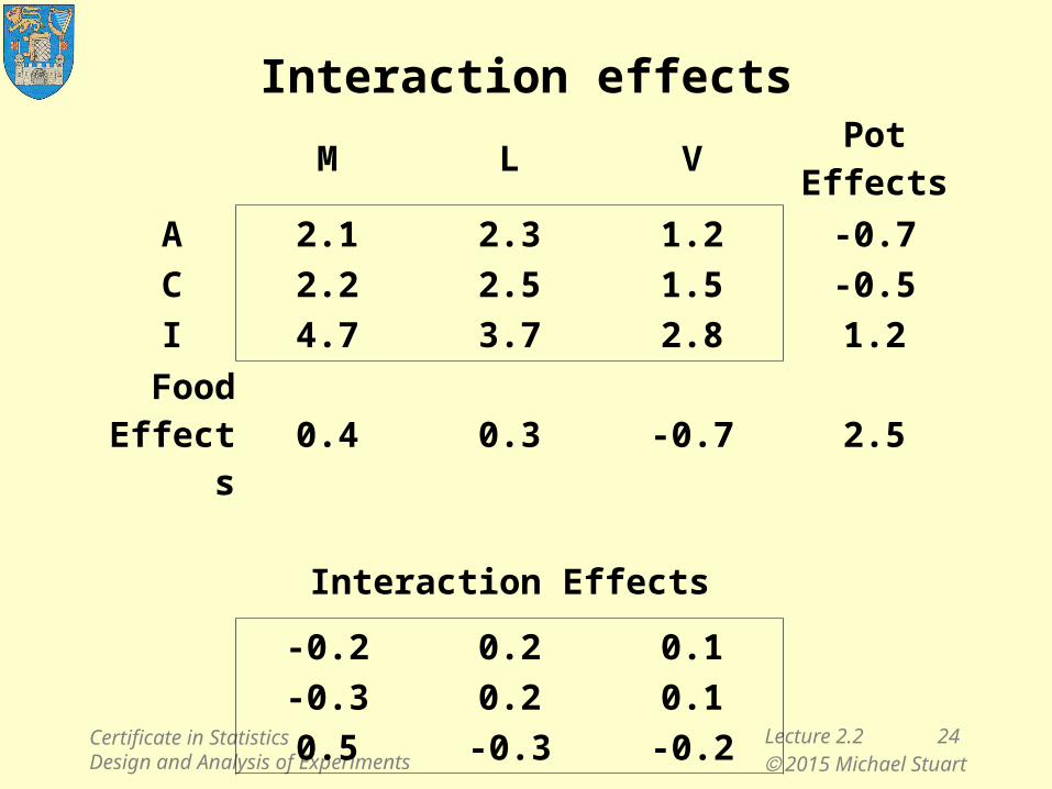
Interaction effects
Certificate in StatisticsDesign and Analysis of Experiments
M L V PotEffects
A 2.1 2.3 1.2 -0.7C 2.2 2.5 1.5 -0.5I 4.7 3.7 2.8 1.2
FoodEffects 0.4 0.3 -0.7 2.5
Interaction Effects
-0.2 0.2 0.1-0.3 0.2 0.10.5 -0.3 -0.2
Lecture 2.2 24 2015 Michael Stuart
Interaction effects
Certificate in StatisticsDesign and Analysis of Experiments
M L V PotEffects
A 2.1 2.3 1.2 -0.7C 2.2 2.5 1.5 -0.5I 4.7 3.7 2.8 1.2
FoodEffects 0.4 0.3 -0.7 2.5
Interaction Effects
-0.2 0.2 0.1-0.3 0.2 0.10.5 -0.3 -0.2
Lecture 2.2 25 2015 Michael Stuart
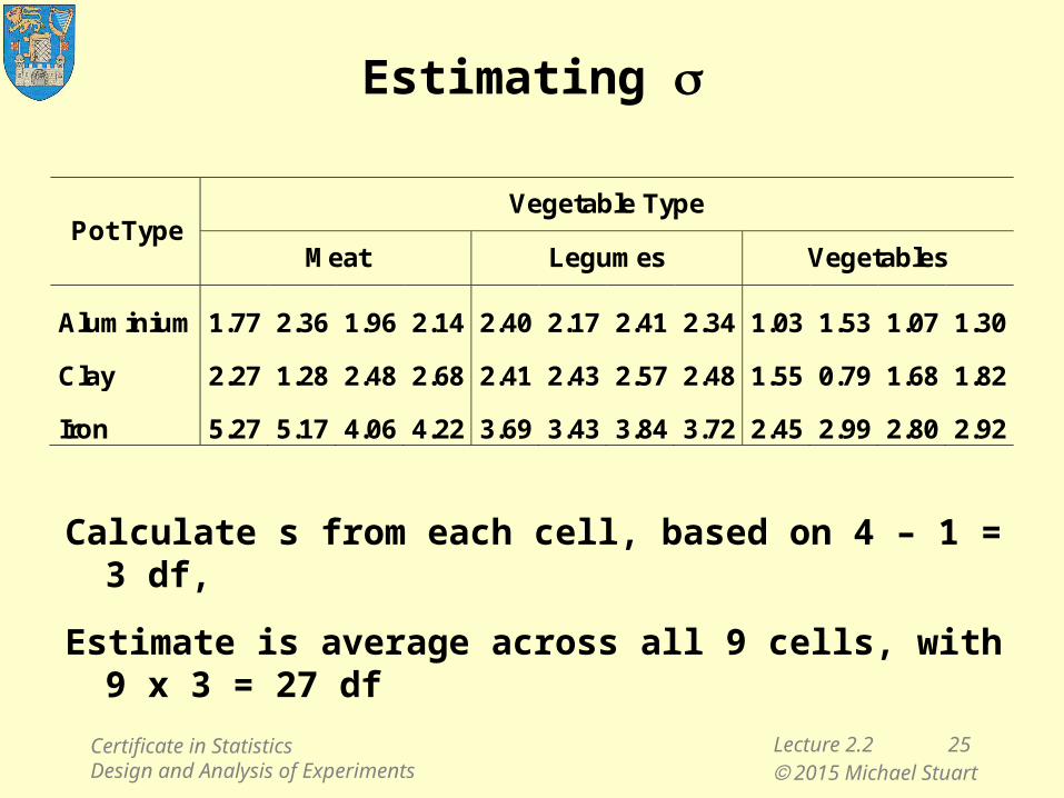
Estimating s
Calculate s from each cell, based on 4 – 1 = 3 df,
Estimate is average across all 9 cells, with 9 x 3 = 27 df
Pot Type Vegetable Type
Meat Legumes Vegetables
Aluminium 1.77 2.36 1.96 2.14 2.40 2.17 2.41 2.34 1.03 1.53 1.07 1.30
Clay 2.27 1.28 2.48 2.68 2.41 2.43 2.57 2.48 1.55 0.79 1.68 1.82
Iron 5.27 5.17 4.06 4.22 3.69 3.43 3.84 3.72 2.45 2.99 2.80 2.92
Certificate in StatisticsDesign and Analysis of Experiments
Lecture 2.2 26 2015 Michael Stuart
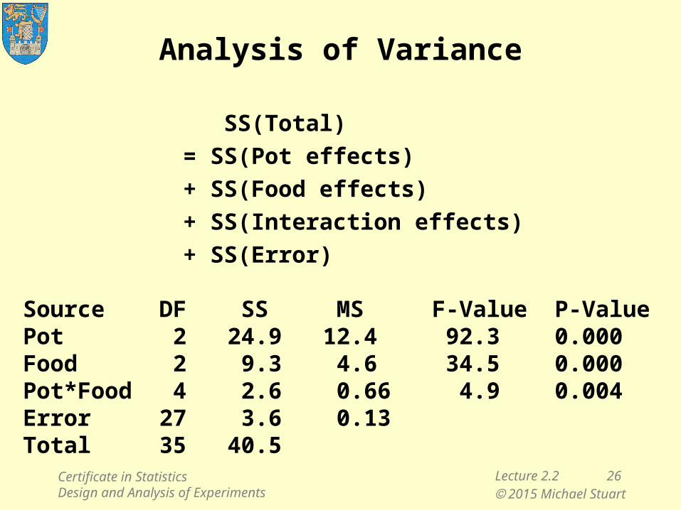
Analysis of Variance
SS(Total)
= SS(Pot effects)
+ SS(Food effects)
+ SS(Interaction effects)
+ SS(Error)
Source DF SS MS F-Value P-ValuePot 2 24.9 12.4 92.3 0.000Food 2 9.3 4.6 34.5 0.000Pot*Food 4 2.6 0.66 4.9 0.004Error 27 3.6 0.13Total 35 40.5
Certificate in StatisticsDesign and Analysis of Experiments
Lecture 2.2 27 2015 Michael Stuart
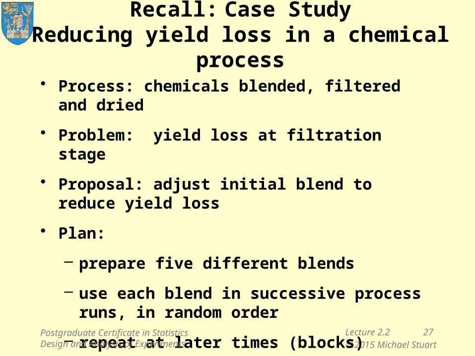
Recall: Case StudyReducing yield loss in a chemical process
• Process: chemicals blended, filtered and dried
• Problem: yield loss at filtration stage
• Proposal: adjust initial blend to reduce yield loss
• Plan:
– prepare five different blends
– use each blend in successive process runs, in random order
– repeat at later times (blocks)
Postgraduate Certificate in Statistics Design and Analysis of Experiments
Lecture 2.2 28 2015 Michael Stuart
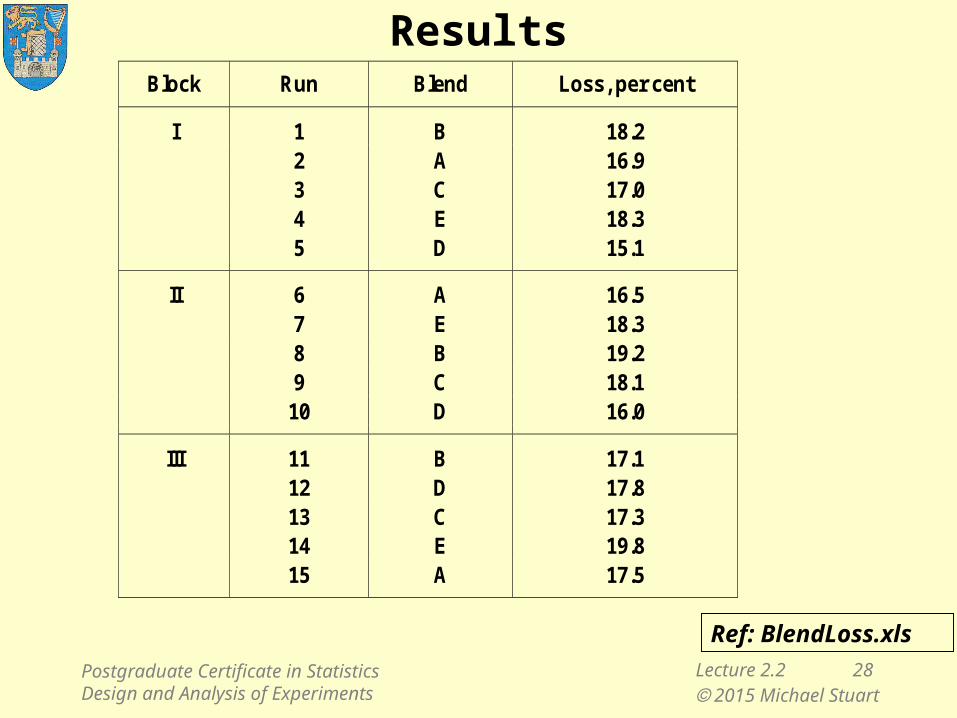
Results
Ref: BlendLoss.xls
Block Run Blend Loss, per cent
I 1 B 18.2 2 A 16.9 3 C 17.0 4 E 18.3 5 D 15.1 II 6 A 16.5 7 E 18.3 8 B 19.2 9 C 18.1 10 D 16.0 III 11 B 17.1 12 D 17.8 13 C 17.3 14 E 19.8 15 A 17.5
Postgraduate Certificate in Statistics Design and Analysis of Experiments
Lecture 2.2 29 2015 Michael Stuart
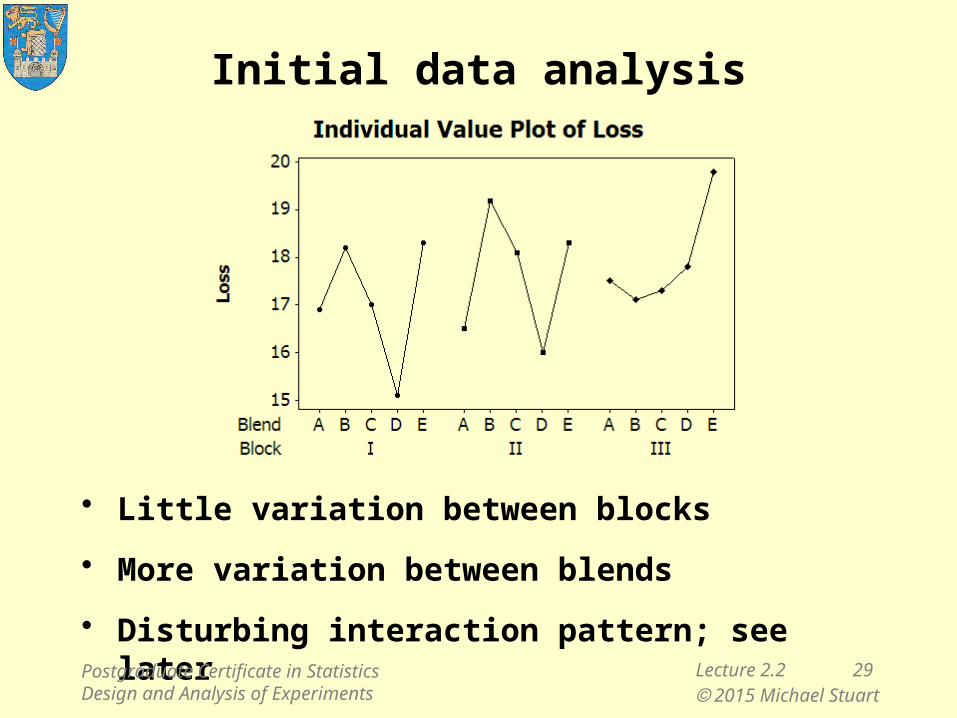
Initial data analysis
• Little variation between blocks
• More variation between blends
• Disturbing interaction pattern; see laterPostgraduate Certificate in Statistics Design and Analysis of Experiments
Lecture 2.2 30 2015 Michael Stuart
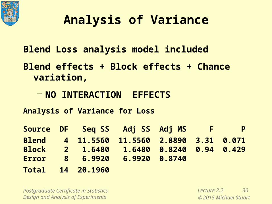
Analysis of Variance
Blend Loss analysis model included
Blend effects + Block effects + Chance variation,
– NO INTERACTION EFFECTS
Analysis of Variance for Loss
Source DF Seq SS Adj SS Adj MS F P
Blend 4 11.5560 11.5560 2.8890 3.31 0.071Block 2 1.6480 1.6480 0.8240 0.94 0.429Error 8 6.9920 6.9920 0.8740
Total 14 20.1960
Postgraduate Certificate in Statistics Design and Analysis of Experiments
Lecture 2.2 31 2015 Michael Stuart
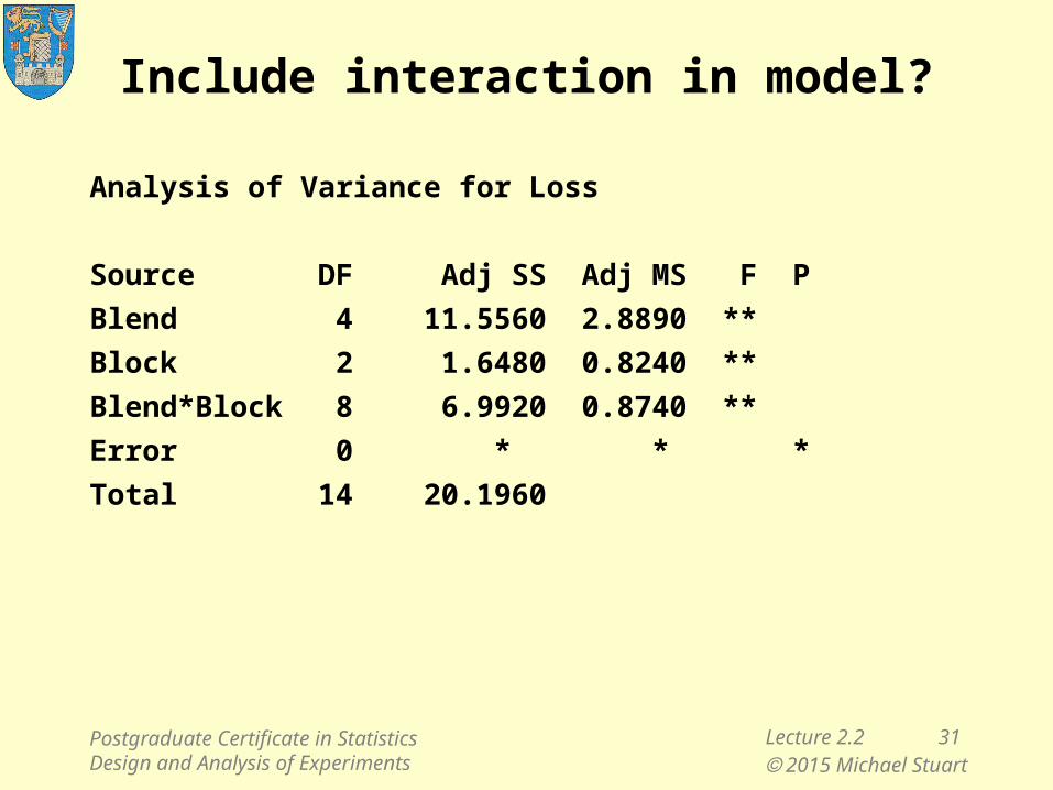
Include interaction in model?
Analysis of Variance for Loss
Source DF Adj SS Adj MS F P
Blend 4 11.5560 2.8890 **
Block 2 1.6480 0.8240 **
Blend*Block 8 6.9920 0.8740 **
Error 0 * * *
Total 14 20.1960
Postgraduate Certificate in Statistics Design and Analysis of Experiments
Lecture 2.2 32 2015 Michael Stuart
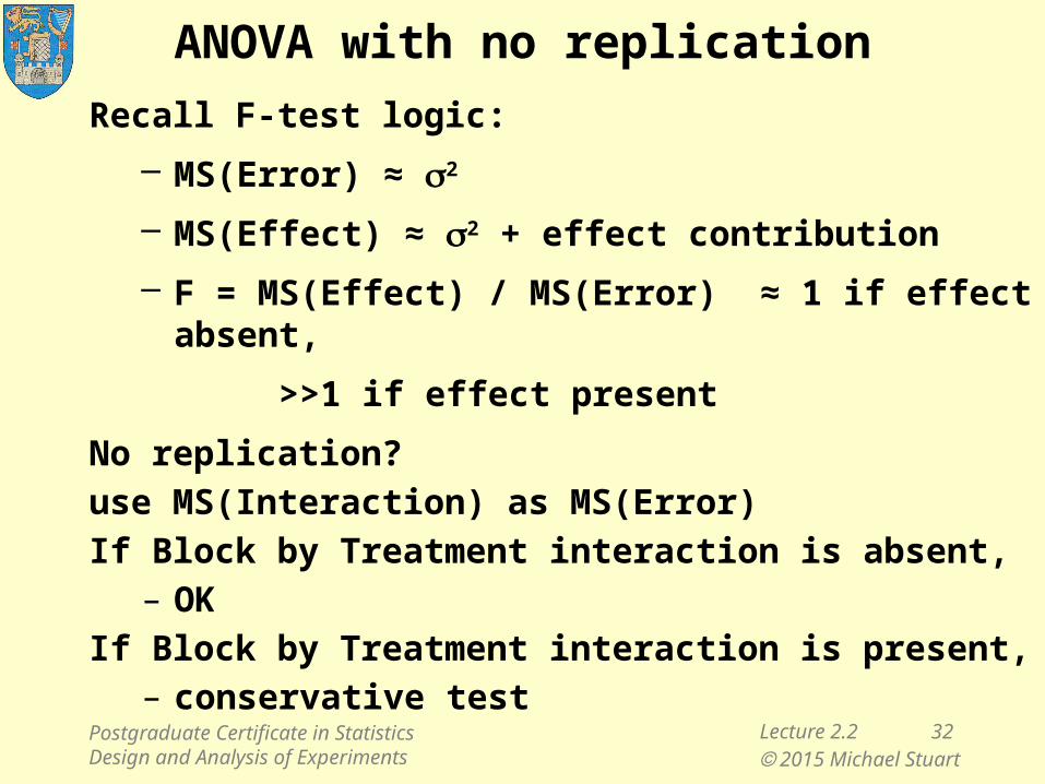
ANOVA with no replication
Recall F-test logic:
– MS(Error) ≈ s2
– MS(Effect) ≈ s2 + effect contribution
– F = MS(Effect) / MS(Error) ≈ 1 if effect absent,
>>1 if effect present
No replication?
use MS(Interaction) as MS(Error)
If Block by Treatment interaction is absent,– OK
If Block by Treatment interaction is present,– conservative test
Postgraduate Certificate in Statistics Design and Analysis of Experiments
Lecture 2.2 33 2015 Michael Stuart
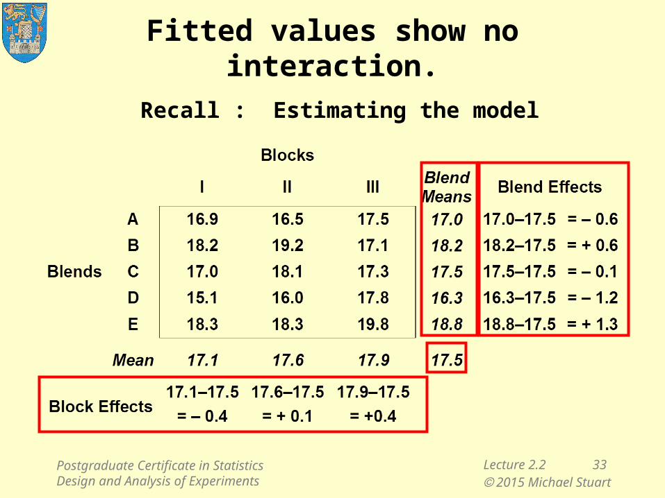
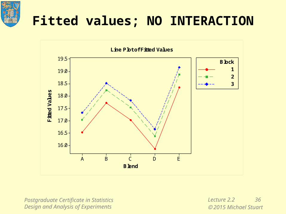
Fitted values show no interaction.
Postgraduate Certificate in Statistics Design and Analysis of Experiments
Recall : Estimating the model
Lecture 2.2 34 2015 Michael Stuart
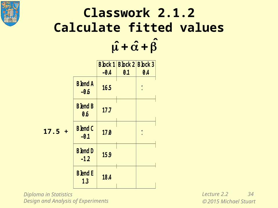
Classwork 2.1.2Calculate fitted values
Diploma in StatisticsDesign and Analysis of Experiments
Block 1
–0.4 Block 2
0.1 Block 3
0.4
Blend A –0.6
16.5 17.0 17.3
Blend B 0.6
17.7 18.2 18.5
Blend C –0.1
17.0 17.5 17.8
Blend D –1.2
15.9 16.4 16.7
Blend E 1.3
18.4 18.9 19.2
ˆˆˆ
17.5 +
Lecture 2.2 35 2015 Michael Stuart
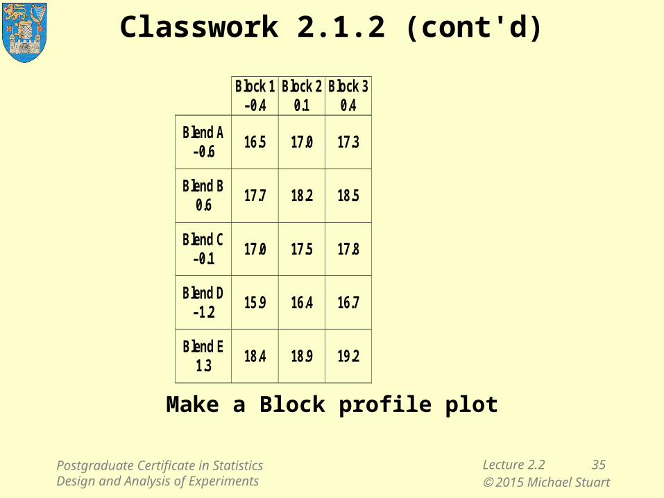
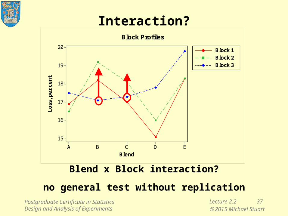
Classwork 2.1.2 (cont'd)
Make a Block profile plot
Block 1
–0.4 Block 2
0.1 Block 3
0.4
Blend A –0.6
16.5 17.0 17.3
Blend B 0.6
17.7 18.2 18.5
Blend C –0.1
17.0 17.5 17.8
Blend D –1.2
15.9 16.4 16.7
Blend E 1.3
18.4 18.9 19.2
Postgraduate Certificate in Statistics Design and Analysis of Experiments
Lecture 2.2 36 2015 Michael Stuart
Fitted values; NO INTERACTION
EDCBA
19.5
19.0
18.5
18.0
17.5
17.0
16.5
16.0
Blend
Fit
ted
Val
ue
s
1
2
3
Block
Line Plot of Fitted Values
Postgraduate Certificate in Statistics Design and Analysis of Experiments
Lecture 2.2 37 2015 Michael Stuart
Interaction?
Blend x Block interaction?
no general test without replication
EDCBA
20
19
18
17
16
15
Blend
Lo
ss, p
er
cen
tBlock 1
Block 2
Block 3
Block Profiles
Postgraduate Certificate in Statistics Design and Analysis of Experiments

Lecture 2.2 38 2015 Michael Stuart
Design and Analysis of ExperimentsLecture 2.2
1. Review Lecture 2.1
– Minute test– Why block?– Deleted residuals
2. Interaction
3. Random Block Effects
4. Introduction to 2-level factorial designs
– a 22 experiment– introducing the Design Matrix
Certificate in StatisticsDesign and Analysis of Experiments
Lecture 2.2 39 2015 Michael Stuart
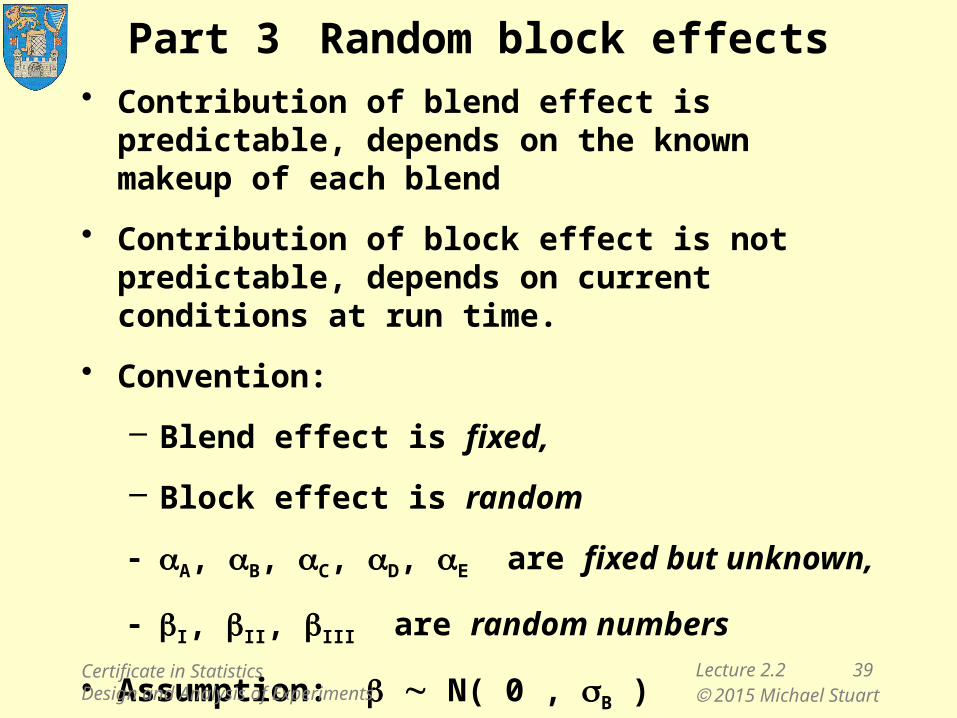
Part 3 Random block effects• Contribution of blend effect is predictable,
depends on the known makeup of each blend
• Contribution of block effect is not predictable, depends on current conditions at run time.
• Convention:
– Blend effect is fixed,
– Block effect is random
aA, aB, aC, aD, aE are fixed but unknown,
bI, bII, bIII are random numbers
• Assumption: b N( 0 , sB )
Certificate in StatisticsDesign and Analysis of Experiments
Lecture 2.2 40 2015 Michael Stuart
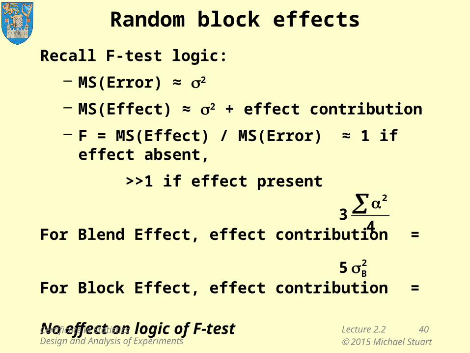
Random block effects
Recall F-test logic:
– MS(Error) ≈ s2
– MS(Effect) ≈ s2 + effect contribution
– F = MS(Effect) / MS(Error) ≈ 1 if effect absent,
>>1 if effect present
For Blend Effect, effect contribution =
For Block Effect, effect contribution =
No effect on logic of F-test
43
2
2B5
Certificate in StatisticsDesign and Analysis of Experiments
Lecture 2.2 41 2015 Michael Stuart
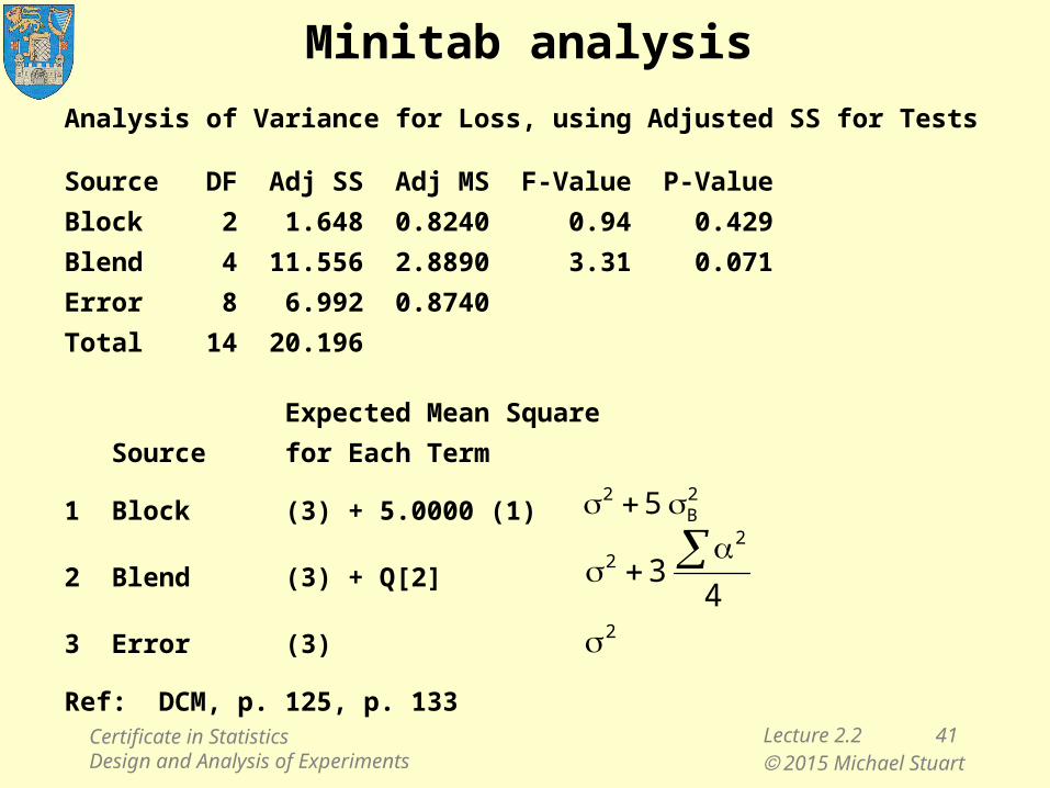
Minitab analysis
Analysis of Variance for Loss, using Adjusted SS for Tests
Source DF Adj SS Adj MS F-Value P-Value
Block 2 1.648 0.8240 0.94 0.429
Blend 4 11.556 2.8890 3.31 0.071
Error 8 6.992 0.8740
Total 14 20.196
Expected Mean Square
Source for Each Term
1 Block (3) + 5.0000 (1)
2 Blend (3) + Q[2]
3 Error (3)
Ref: DCM, p. 125, p. 133
43
22
2B
2 5
2
Certificate in StatisticsDesign and Analysis of Experiments
Lecture 2.2 42 2015 Michael Stuart
Design and Analysis of ExperimentsLecture 2.2
1. Review Lecture 2.1
– Minute test– Why block?– Deleted residuals
2. Interaction
3. Random Block Effects
4. Introduction to 2-level factorial designs
– a 22 experiment– introducing the Design Matrix
Certificate in StatisticsDesign and Analysis of Experiments
Lecture 2.2 43 2015 Michael Stuart
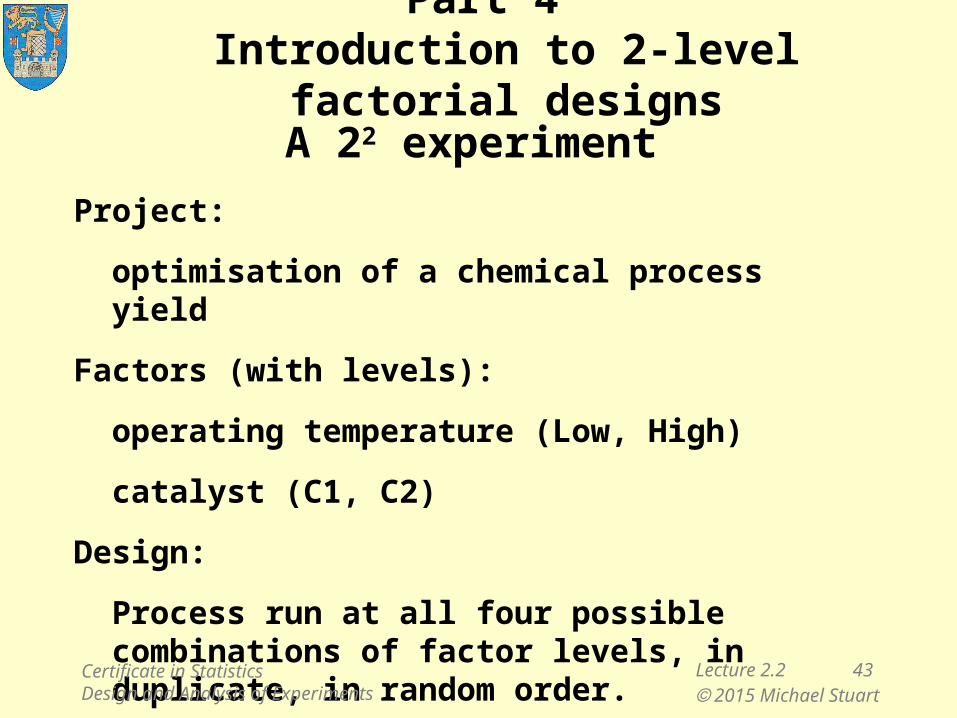
Part 4Introduction to 2-level factorial designs
A 22 experiment
Project:
optimisation of a chemical process yield
Factors (with levels):
operating temperature (Low, High)
catalyst (C1, C2)
Design:
Process run at all four possible combinations of factor levels, in duplicate, in random order.
Certificate in StatisticsDesign and Analysis of Experiments
Lecture 2.2 44 2015 Michael Stuart
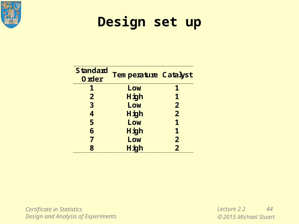
Standard Order
Temperature Catalyst
1 Low 1 2 High 1 3 Low 2 4 High 2 5 Low 1 6 High 1 7 Low 2 8 High 2
Design set up
Certificate in StatisticsDesign and Analysis of Experiments

Lecture 2.2 45 2015 Michael Stuart
Go to Excel
Standard Order
Temperature Catalyst Run
Order 1 Low 1 6 2 High 1 8 3 Low 2 1 4 High 2 4 5 Low 1 3 6 High 1 7 7 Low 2 2 8 High 2 5
Randomisation
Certificate in StatisticsDesign and Analysis of Experiments
Lecture 2.2 46 2015 Michael Stuart
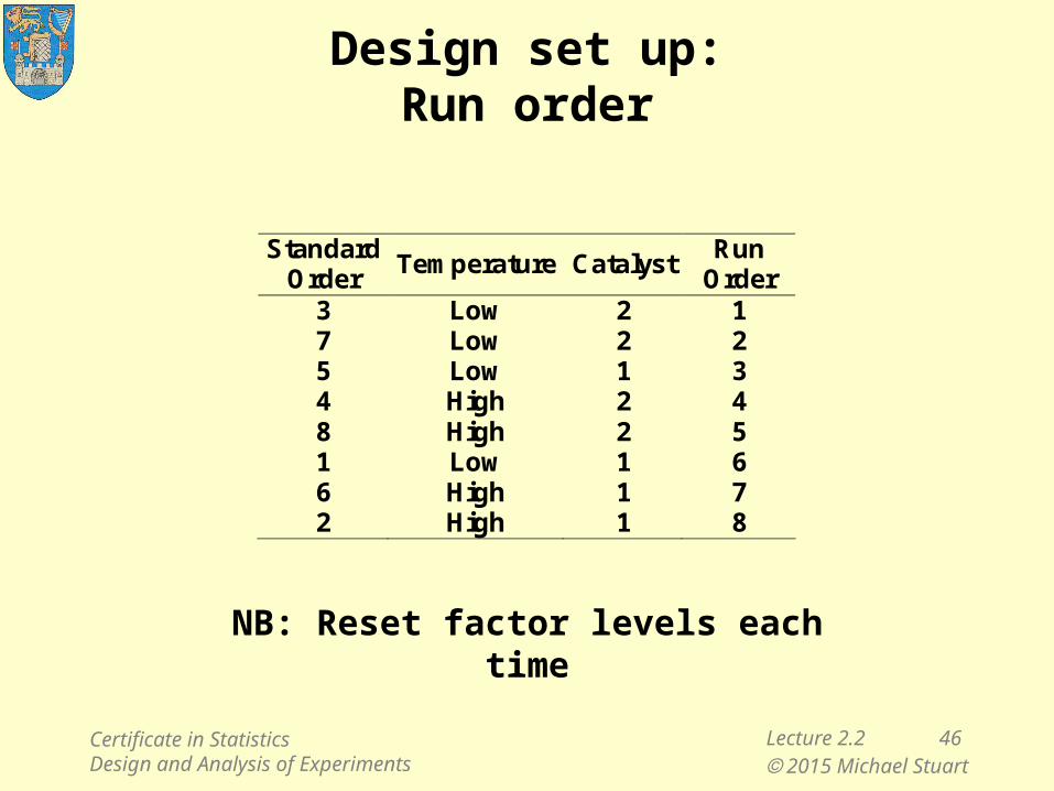
Design set up:Run order
Standard Order
Temperature Catalyst Run
Order 3 Low 2 1 7 Low 2 2 5 Low 1 3 4 High 2 4 8 High 2 5 1 Low 1 6 6 High 1 7 2 High 1 8
NB: Reset factor levels each time
Certificate in StatisticsDesign and Analysis of Experiments
Lecture 2.2 47 2015 Michael Stuart
Classwork 2.2.3
What were the
experimental units
factors
factor levels
treatments
response
blocks
allocation procedure
Certificate in StatisticsDesign and Analysis of Experiments
Lecture 2.2 48 2015 Michael Stuart
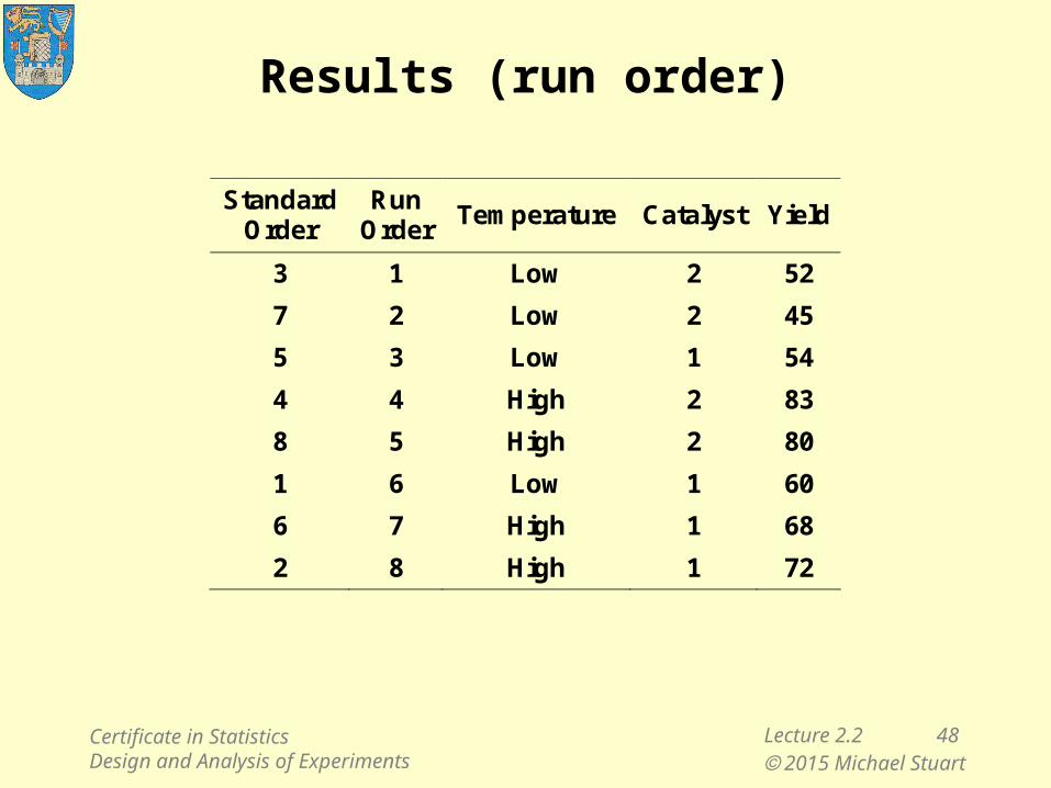
Results (run order)
Standard Order
Run Order
Temperature Catalyst Yield
3 1 Low 2 52
7 2 Low 2 45
5 3 Low 1 54
4 4 High 2 83
8 5 High 2 80
1 6 Low 1 60
6 7 High 1 68
2 8 High 1 72
Certificate in StatisticsDesign and Analysis of Experiments
Lecture 2.2 49 2015 Michael Stuart
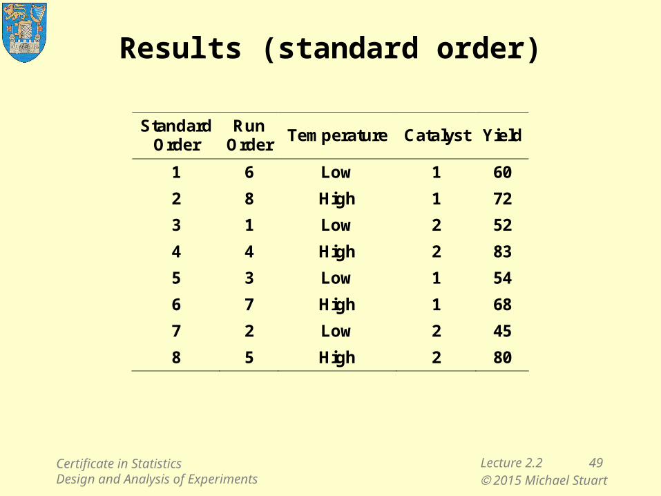
Results (standard order)
Standard Order
Run Order
Temperature Catalyst Yield
1 6 Low 1 60
2 8 High 1 72
3 1 Low 2 52
4 4 High 2 83
5 3 Low 1 54
6 7 High 1 68
7 2 Low 2 45
8 5 High 2 80
Certificate in StatisticsDesign and Analysis of Experiments
Lecture 2.2 50 2015 Michael Stuart
Analysis (Minitab)
• Main effects and Interaction plots
• ANOVA results
– with diagnostics
• Calculation of t-statistics
Certificate in StatisticsDesign and Analysis of Experiments

Lecture 2.2 51 2015 Michael Stuart
HighLow
75
70
65
60
55
50
21
Temperature
Mea
n
Catalyst
21
85
80
75
70
65
60
55
50
CatalystM
ean
Low
High
Temperature
Main Effects Plot for YieldData Means
Interaction Plot for YieldData Means
Main Effects and Interactions
Certificate in StatisticsDesign and Analysis of Experiments
Lecture 2.2 52 2015 Michael Stuart
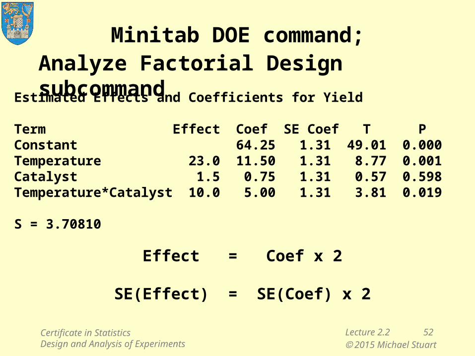
Minitab DOE command;
Estimated Effects and Coefficients for Yield
Term Effect Coef SE Coef T PConstant 64.25 1.31 49.01 0.000Temperature 23.0 11.50 1.31 8.77 0.001Catalyst 1.5 0.75 1.31 0.57 0.598Temperature*Catalyst 10.0 5.00 1.31 3.81 0.019
S = 3.70810
Effect = Coef x 2
SE(Effect) = SE(Coef) x 2
Analyze Factorial Design subcommand
Certificate in StatisticsDesign and Analysis of Experiments
Lecture 2.2 53 2015 Michael Stuart
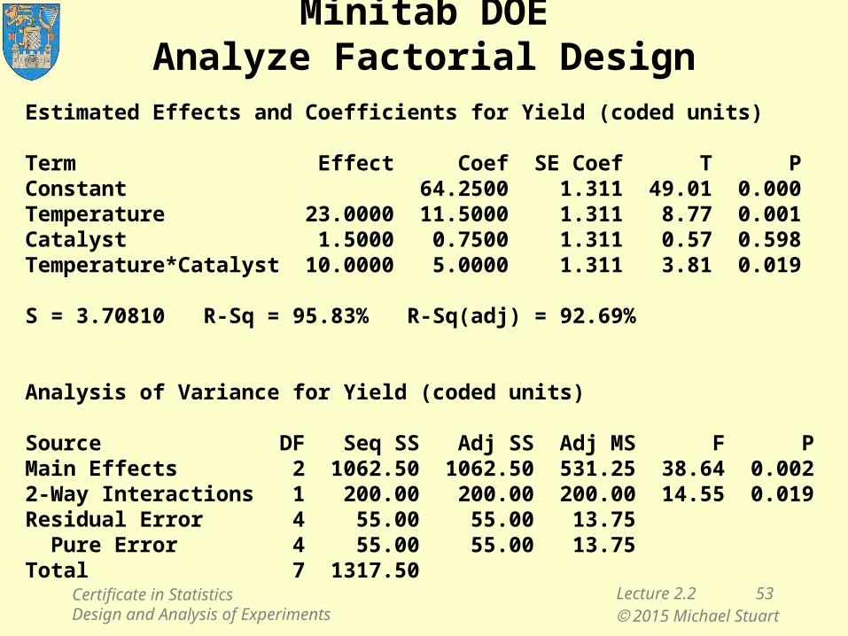
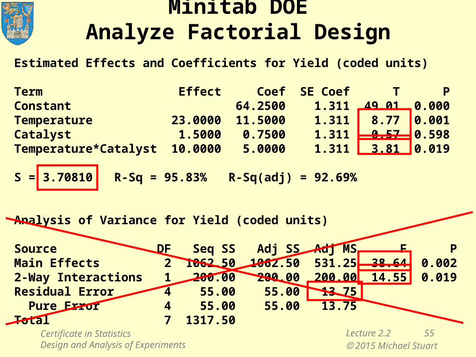
Minitab DOEAnalyze Factorial Design
Estimated Effects and Coefficients for Yield (coded units)
Term Effect Coef SE Coef T PConstant 64.2500 1.311 49.01 0.000Temperature 23.0000 11.5000 1.311 8.77 0.001Catalyst 1.5000 0.7500 1.311 0.57 0.598Temperature*Catalyst 10.0000 5.0000 1.311 3.81 0.019
S = 3.70810 R-Sq = 95.83% R-Sq(adj) = 92.69%
Analysis of Variance for Yield (coded units)
Source DF Seq SS Adj SS Adj MS F PMain Effects 2 1062.50 1062.50 531.25 38.64 0.0022-Way Interactions 1 200.00 200.00 200.00 14.55 0.019Residual Error 4 55.00 55.00 13.75 Pure Error 4 55.00 55.00 13.75Total 7 1317.50
Certificate in StatisticsDesign and Analysis of Experiments
Lecture 2.2 54 2015 Michael Stuart
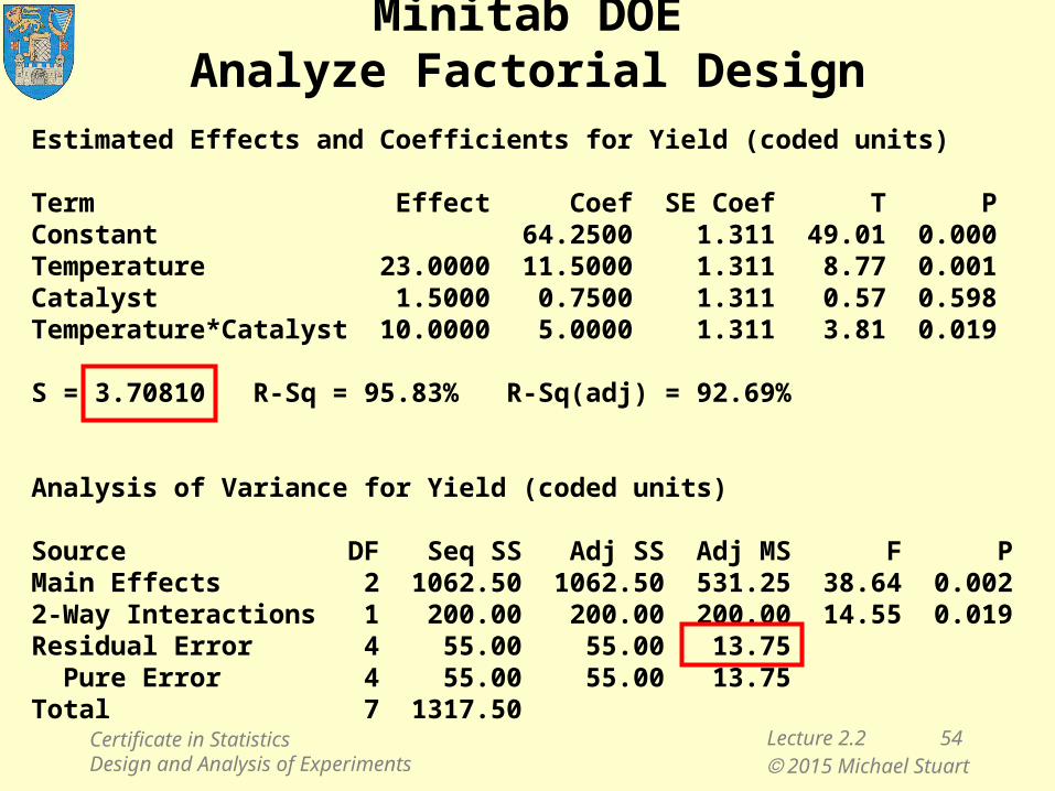
Minitab DOEAnalyze Factorial Design
Estimated Effects and Coefficients for Yield (coded units)
Term Effect Coef SE Coef T PConstant 64.2500 1.311 49.01 0.000Temperature 23.0000 11.5000 1.311 8.77 0.001Catalyst 1.5000 0.7500 1.311 0.57 0.598Temperature*Catalyst 10.0000 5.0000 1.311 3.81 0.019
S = 3.70810 R-Sq = 95.83% R-Sq(adj) = 92.69%
Analysis of Variance for Yield (coded units)
Source DF Seq SS Adj SS Adj MS F PMain Effects 2 1062.50 1062.50 531.25 38.64 0.0022-Way Interactions 1 200.00 200.00 200.00 14.55 0.019Residual Error 4 55.00 55.00 13.75 Pure Error 4 55.00 55.00 13.75Total 7 1317.50
Certificate in StatisticsDesign and Analysis of Experiments
Lecture 2.2 55 2015 Michael Stuart
Minitab DOEAnalyze Factorial Design
Estimated Effects and Coefficients for Yield (coded units)
Term Effect Coef SE Coef T PConstant 64.2500 1.311 49.01 0.000Temperature 23.0000 11.5000 1.311 8.77 0.001Catalyst 1.5000 0.7500 1.311 0.57 0.598Temperature*Catalyst 10.0000 5.0000 1.311 3.81 0.019
S = 3.70810 R-Sq = 95.83% R-Sq(adj) = 92.69%
Analysis of Variance for Yield (coded units)
Source DF Seq SS Adj SS Adj MS F PMain Effects 2 1062.50 1062.50 531.25 38.64 0.0022-Way Interactions 1 200.00 200.00 200.00 14.55 0.019Residual Error 4 55.00 55.00 13.75 Pure Error 4 55.00 55.00 13.75Total 7 1317.50
Certificate in StatisticsDesign and Analysis of Experiments
Lecture 2.2 56 2015 Michael Stuart
ANOVA results
ANOVA superfluous for 2k experiments
"There is nothing to justify this complexity other than a misplaced belief in the universal value of an ANOVA table".
BHH, Section 5.10, p.188
“The standard form of the ‘analysis of variance’ • • • does not seem to me to be useful for 2n data.
Daniel (1976), Section 7.1, p.128
Certificate in StatisticsDesign and Analysis of Experiments
Lecture 2.2 57 2015 Michael Stuart
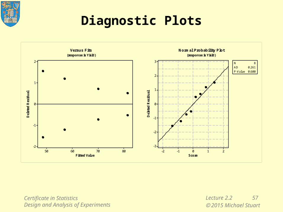
Diagnostic Plots
80706050
2
1
0
-1
-2
Fitted Value
Del
eted
Res
idu
al
3
2
1
0
-1
-2
-3
210-1-2D
elet
ed R
esid
ual
Score
N 8
AD 0.261
P-Value 0.600
Versus Fits(response is Yield)
Normal Probability Plot(response is Yield)
Certificate in StatisticsDesign and Analysis of Experiments
Lecture 2.2 58 2015 Michael Stuart
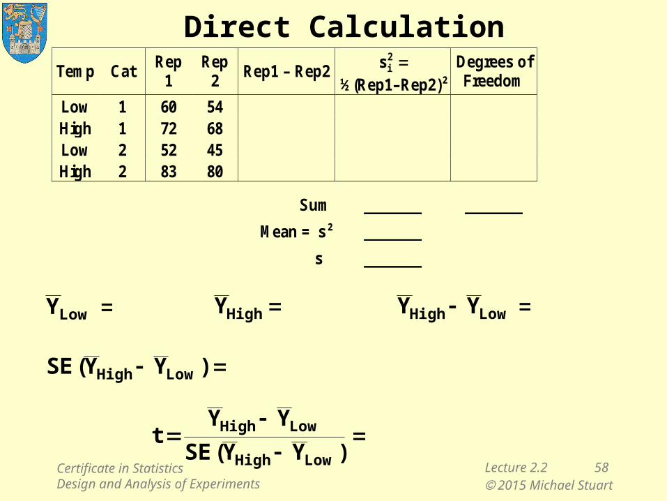
Direct CalculationTemp Cat
Rep 1
Rep 2
Rep1 – Rep2 2is
½(Rep1–Rep2)² Degrees of Freedom
Low 1 60 54 High 1 72 68 Low 2 52 45 High 2 83 80
Sum
Mean = s²
s
LowY HighY LowHigh YY
)YY(SE LowHigh
)YY(SE
YYt
LowHigh
LowHigh
Certificate in StatisticsDesign and Analysis of Experiments
Lecture 2.2 59 2015 Michael Stuart
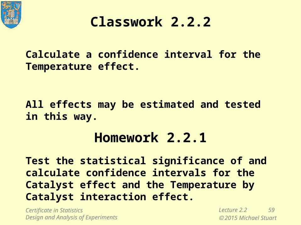
Classwork 2.2.2
Calculate a confidence interval for the Temperature effect.
All effects may be estimated and tested in this way.
Homework 2.2.1
Test the statistical significance of and calculate confidence intervals for the Catalyst effect and the Temperature by Catalyst interaction effect.
Certificate in StatisticsDesign and Analysis of Experiments
Lecture 2.2 60 2015 Michael Stuart
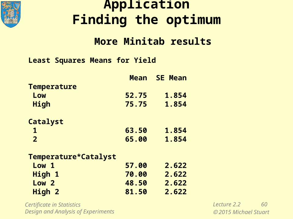
ApplicationFinding the optimum
More Minitab results
Least Squares Means for Yield
Mean SE MeanTemperature Low 52.75 1.854 High 75.75 1.854
Catalyst 1 63.50 1.854 2 65.00 1.854
Temperature*Catalyst Low 1 57.00 2.622 High 1 70.00 2.622 Low 2 48.50 2.622 High 2 81.50 2.622
Certificate in StatisticsDesign and Analysis of Experiments
Lecture 2.2 61 2015 Michael Stuart
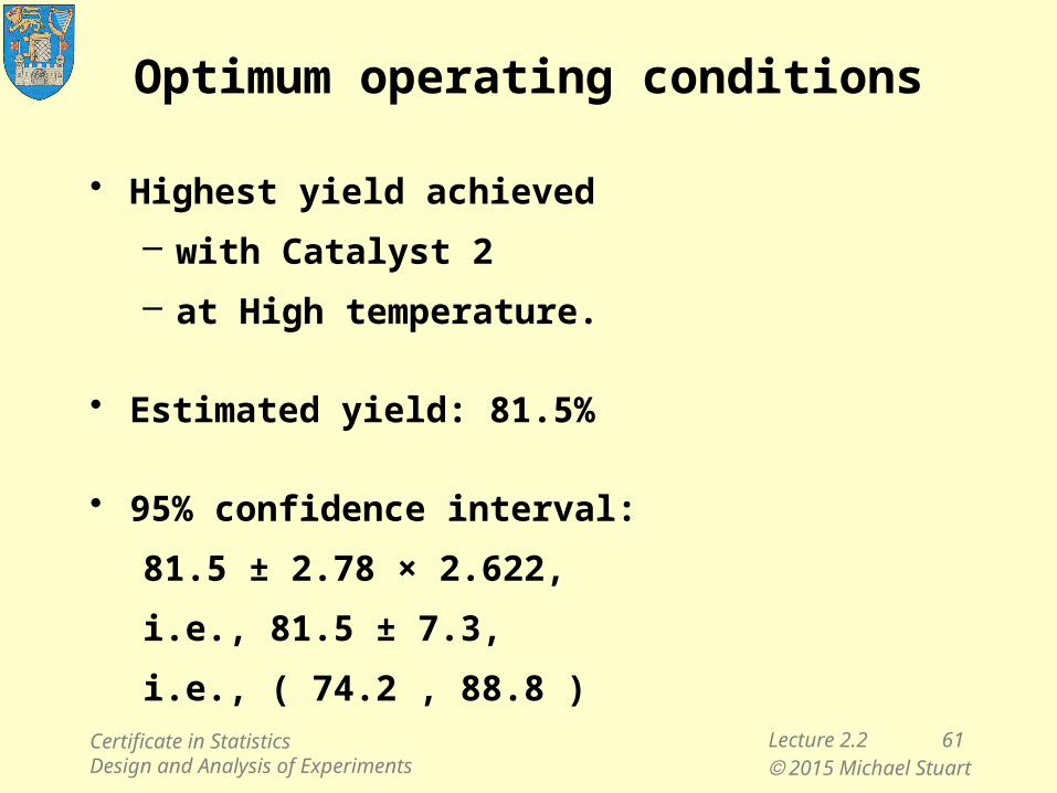
Optimum operating conditions
• Highest yield achieved
– with Catalyst 2
– at High temperature.
• Estimated yield: 81.5%
• 95% confidence interval:
81.5 ± 2.78 × 2.622,
i.e., 81.5 ± 7.3,
i.e., ( 74.2 , 88.8 )Certificate in StatisticsDesign and Analysis of Experiments
Lecture 2.2 62 2015 Michael Stuart
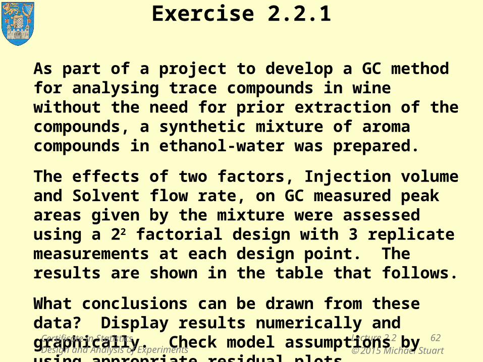
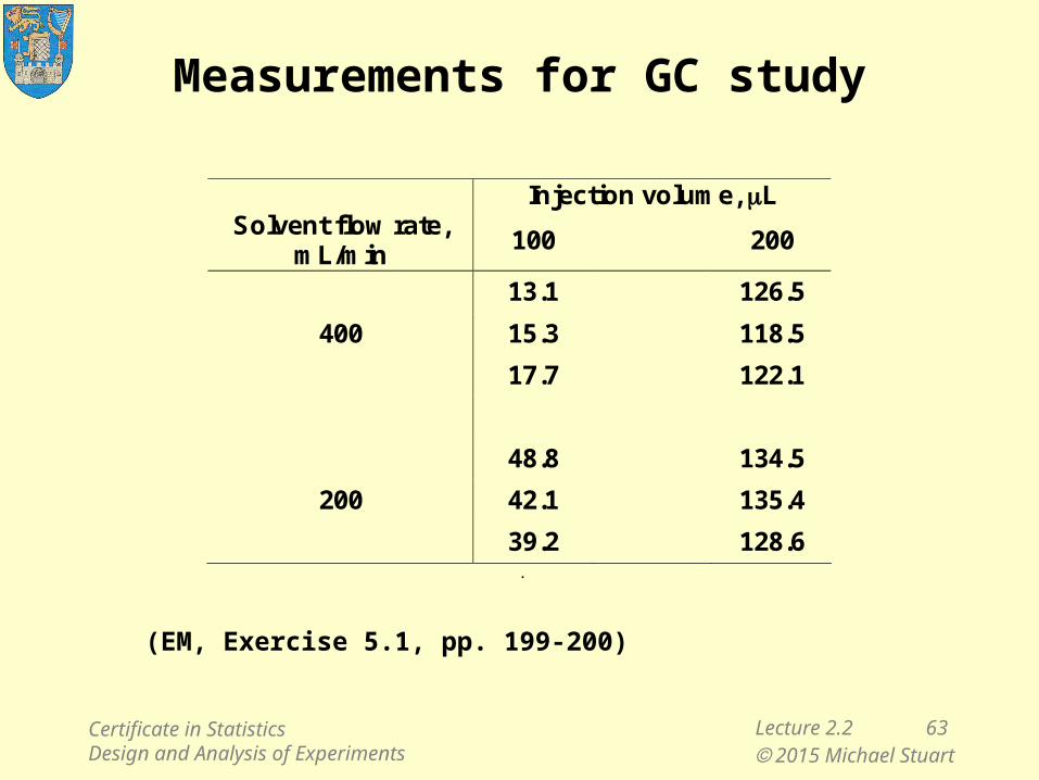
Exercise 2.2.1
As part of a project to develop a GC method for analysing trace compounds in wine without the need for prior extraction of the compounds, a synthetic mixture of aroma compounds in ethanol-water was prepared.
The effects of two factors, Injection volume and Solvent flow rate, on GC measured peak areas given by the mixture were assessed using a 22 factorial design with 3 replicate measurements at each design point. The results are shown in the table that follows.
What conclusions can be drawn from these data? Display results numerically and graphically. Check model assumptions by using appropriate residual plots.
Certificate in StatisticsDesign and Analysis of Experiments
Lecture 2.2 63 2015 Michael Stuart
Measurements for GC study
Injection volume, L Solvent flow rate,
mL/min 100 200
13.1 126.5
400 15.3 118.5
17.7 122.1
48.8 134.5
200 42.1 135.4
39.2 128.6 .
(EM, Exercise 5.1, pp. 199-200)
Certificate in StatisticsDesign and Analysis of Experiments
Lecture 2.2 64 2015 Michael Stuart
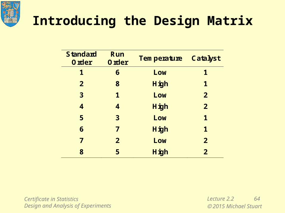
Introducing the Design Matrix
Standard Order
Run Order
Temperature Catalyst
1 6 Low 1
2 8 High 1
3 1 Low 2
4 4 High 2
5 3 Low 1
6 7 High 1
7 2 Low 2
8 5 High 2
Certificate in StatisticsDesign and Analysis of Experiments
Lecture 2.2 65 2015 Michael Stuart
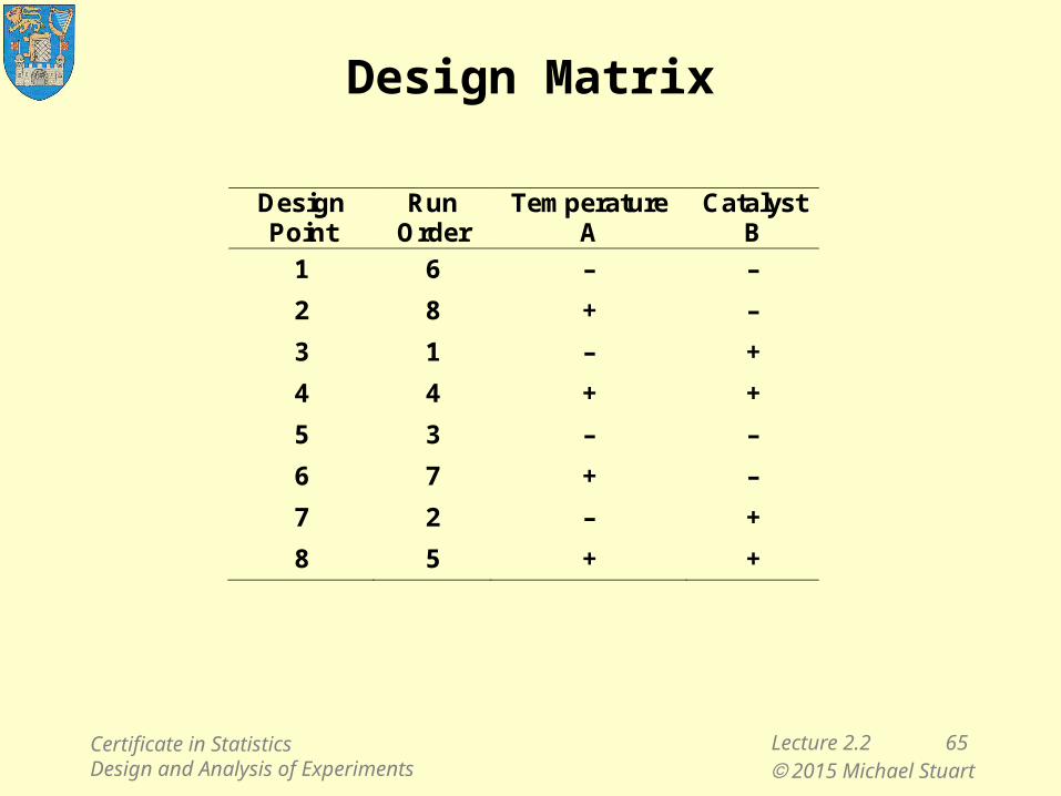
Design Matrix
Design Point
Run Order
Temperature A
Catalyst B
1 6 – –
2 8 + –
3 1 – +
4 4 + +
5 3 – –
6 7 + –
7 2 – +
8 5 + +
Certificate in StatisticsDesign and Analysis of Experiments
Lecture 2.2 66 2015 Michael Stuart
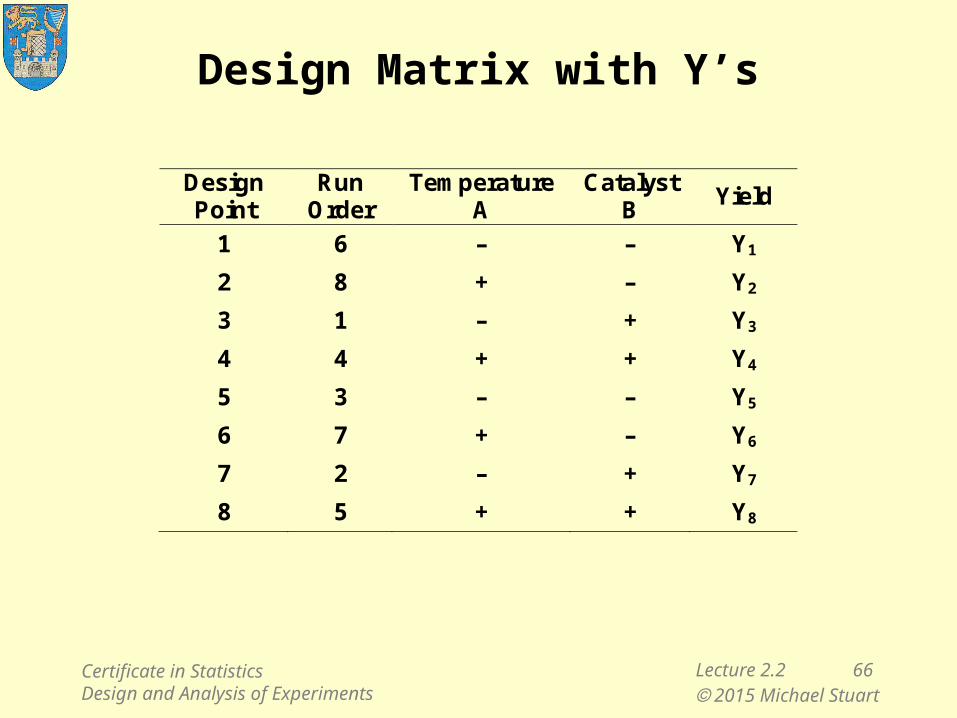
Design Matrix with Y’s
Design Point
Run Order
Temperature A
Catalyst B
Yield
1 6 – – Y1
2 8 + – Y2
3 1 – + Y3
4 4 + + Y4
5 3 – – Y5
6 7 + – Y6
7 2 – + Y7
8 5 + + Y8
Certificate in StatisticsDesign and Analysis of Experiments
Lecture 2.2 67 2015 Michael Stuart
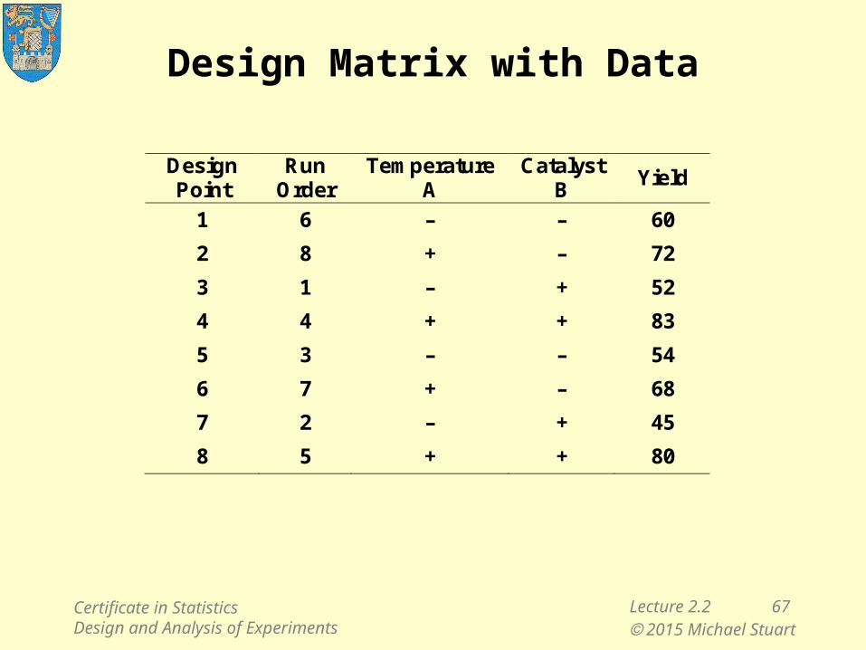
Design Matrix with Data
Design Point
Run Order
Temperature A
Catalyst B
Yield
1 6 – – 60
2 8 + – 72
3 1 – + 52
4 4 + + 83
5 3 – – 54
6 7 + – 68
7 2 – + 45
8 5 + + 80
Certificate in StatisticsDesign and Analysis of Experiments
Lecture 2.2 68 2015 Michael Stuart
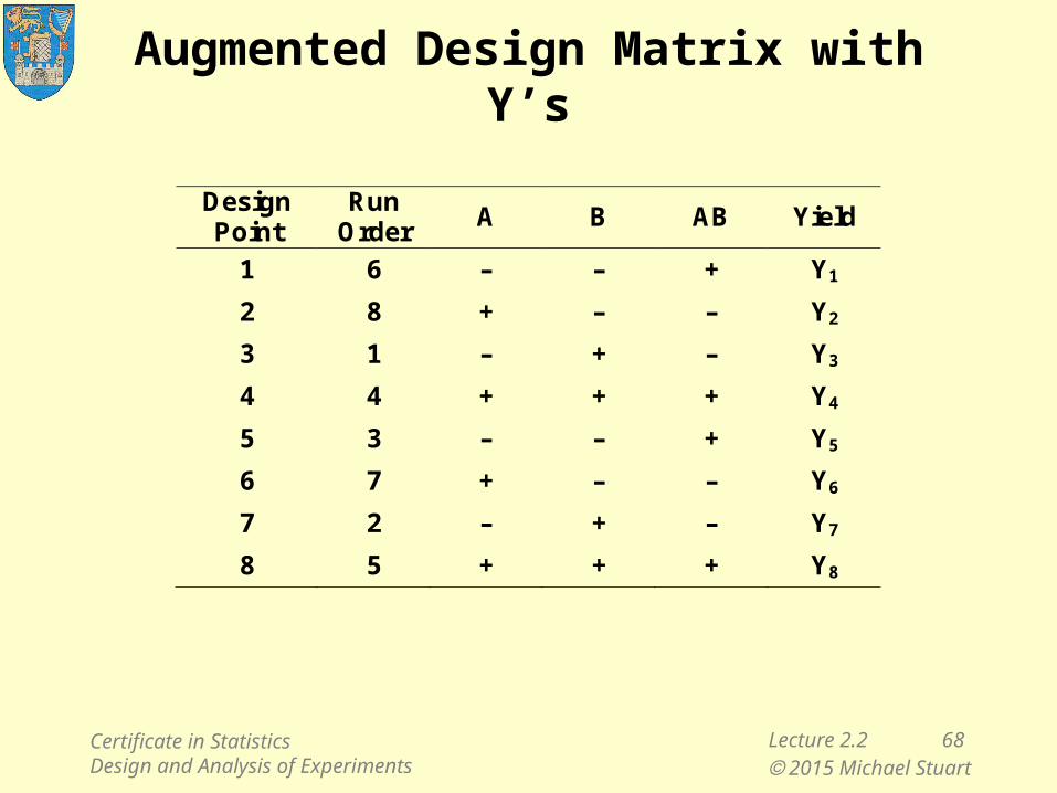
Augmented Design Matrix with Y’s
Design Point
Run Order
A B AB Yield
1 6 – – + Y1
2 8 + – – Y2
3 1 – + – Y3
4 4 + + + Y4
5 3 – – + Y5
6 7 + – – Y6
7 2 – + – Y7
8 5 + + + Y8
Certificate in StatisticsDesign and Analysis of Experiments
Lecture 2.2 69 2015 Michael Stuart
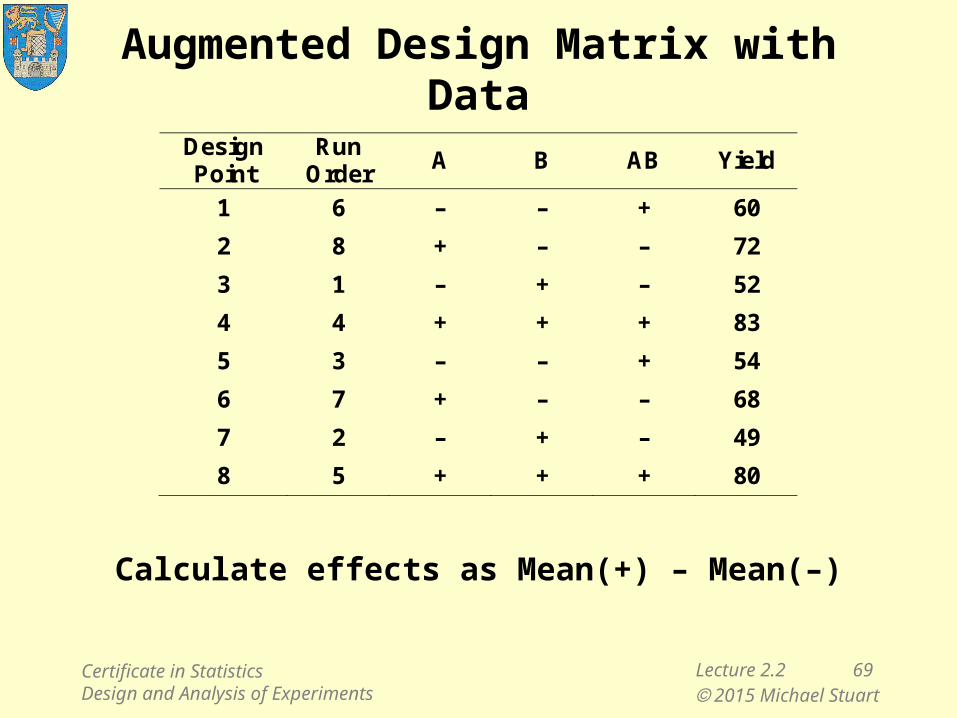
Augmented Design Matrix with Data
Calculate effects as Mean(+) – Mean(–)
Design Point
Run Order
A B AB Yield
1 6 – – + 60
2 8 + – – 72
3 1 – + – 52
4 4 + + + 83
5 3 – – + 54
6 7 + – – 68
7 2 – + – 49
8 5 + + + 80
Certificate in StatisticsDesign and Analysis of Experiments
Lecture 2.2 70 2015 Michael Stuart
Dual role of the design matrix
• Prior to the experiment, the rows designate the design points, the sets of conditions under which the process is to be run.
• After the experiment, the columns designate the contrasts, the combinations of design point means which measure the main effects of the factors.
• The extended design matrix facilitates the calculation of interaction effects
Certificate in StatisticsDesign and Analysis of Experiments
Lecture 2.2 71 2015 Michael Stuart
Reading
EM §5.3
DCM §6-2, §6-2
Certificate in StatisticsDesign and Analysis of Experiments