Embed Size (px)
Citation preview

Transformations: I
• Forbes happily had a physical argument to justify linear model
E(log (pressure) | boiling point) = �0 + �1 ⇥ boiling point
• usual (not so happy) situation: parametric model behind MLRis convenient approximation at best
� “All models are wrong but some are useful.” (Box, 1979)
• transformations allow MLR models to be extended to data that,in their original state, are poorly approximated by linear models
• in SLR case, idea is to get transformation eY of response Yand/or transformation eX of regressor X such that
E(eY | eX = x) ⇡ �0 + �1x
ALR–185 VIII–1

Transformations: II
• while transformations are a favorite tool of statisticians, theiruse is not without controversy (arises in the physical sciences)
• picking suitable transformations is part science and part art
• focusing on SLR to start with, need for transformation is man-ifested in nonlinear appearance of scatterplot
• let’s look at two examples from Weisberg:
� height of cedar trees (response) versus diameter at 4.5 feetabove the ground (regressor) – see Figure 8.3 (p. 190)
� surface tension of liquid copper (response) versus dissolvedsulfur (regressor) – see Problem 8.1 (pp. 199–200)
ALR–189, 190, 199, 200 VIII–2

Scatterplot for Cedar Tree Example
200 400 600 800 1000
100
150
200
250
300
350
400
Dbh (mm)
Hei
ght (
dm)
ALR–189, 190 VIII–3

Scatterplot for Liquid Copper Example
0.2 0.4 0.6 0.8
300
400
500
600
700
Sulfur (% of weight)
Tens
ion
(dyn
es/c
m)
ALR–199, 200 VIII–4

Transforming One Regressor: I
• assuming regressor is positive (true for two examples), widelyused family of transformations is scaled power transformations:
S(X,�) =
((X� � 1)/�, � 6= 0
log(X), � = 0
• rationale for �1 and division by � for � 6= 0 is in part tied todefinition for � = 0 choice: can show that
lim�!0
X� � 1
�= log(X)
by making use of
X� � 1
�=
e� log(X) � 1
�along with ez = 1 + z +
z2
2!+
z3
3!+ · · ·
ALR–189 VIII–5

Transforming One Regressor: II
• for � = 0, E(Y | X = x) = �0 + �1 log(x), whereas, for � 6= 0,
E(Y | X = x) = �0 + �1x� � 1
�
= �0 ��1
�+�1
�x�
= ↵0 + ↵1x�,
where ↵0 = �0 � �1� and ↵1 = �1
�
• in practice unscaled power transformation achieves same e↵ect:
(X,�) =
(X�, � 6= 0
log(X), � = 0
� note: (X,�) has opposite sign from S(X,�) when � < 0
• choice � = 1 is essentially no transformation
ALR–189, 186 VIII–6

Transforming One Regressor: III
• idea is to find � such that we approximately have
E(Y | X = x) = �0 + �1 S(x,�)
• given data (xi, yi), consider residual sum of squares function:
RSS(b0, b1,�) =nX
i=1
[yi � (b0 + b1 S(xi,�))]2
• for fixed �, minimizer of above is OLS estimators �0 and �1from regression of yi on S(xi,�), resulting in
RSS(�) = RSS(�0, �1,�)
ALR–189 VIII–7

Transforming One Regressor: IV
• idea: select � such that RSS(�) is minimized over �
• in theory, need nonlinear optimizer to find best �, but, since wereally don’t need to know � precisely, can often make do withrestricted grid search using, e.g.,
� 2n�2,�1,�1
2,�13, 0,
13,
12, 1, 2
o
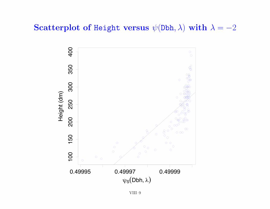
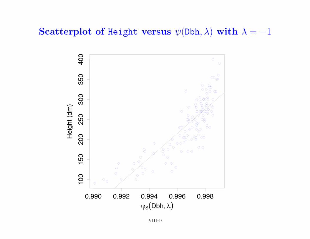
• returning to cedar tree example, following scatterplots showHeight versus (Dbh,�) along with fitted regression line forabove 9 choices of �
ALR–189 VIII–8
Scatterplot of Height versus (Dbh,�) with � = �2
0.49995 0.49997 0.49999
100
150
200
250
300
350
400
sS(Dbh, h)
Hei
ght (
dm)
VIII–9
Scatterplot of Height versus (Dbh,�) with � = �1
0.990 0.992 0.994 0.996 0.998
100
150
200
250
300
350
400
sS(Dbh, h)
Hei
ght (
dm)
VIII–9

Scatterplot of Height versus (Dbh,�) with � = �1/2
1.80 1.84 1.88 1.92
100
150
200
250
300
350
400
sS(Dbh, h)
Hei
ght (
dm)
VIII–9
Scatterplot of Height versus (Dbh,�) with � = �1/3
2.35 2.45 2.55 2.65
100
150
200
250
300
350
400
sS(Dbh, h)
Hei
ght (
dm)
VIII–9

Scatterplot of Height versus (Dbh,�) with � = 0
5.0 5.5 6.0 6.5 7.0
100
150
200
250
300
350
400
sS(Dbh, h)
Hei
ght (
dm)
ALR–191 VIII–9

Scatterplot of Height versus (Dbh,�) with � = 1/3
15 20 25
100
150
200
250
300
350
400
sS(Dbh, h)
Hei
ght (
dm)
VIII–10

Scatterplot of Height versus (Dbh,�) with � = 1/2
20 30 40 50 60
100
150
200
250
300
350
400
sS(Dbh, h)
Hei
ght (
dm)
VIII–10
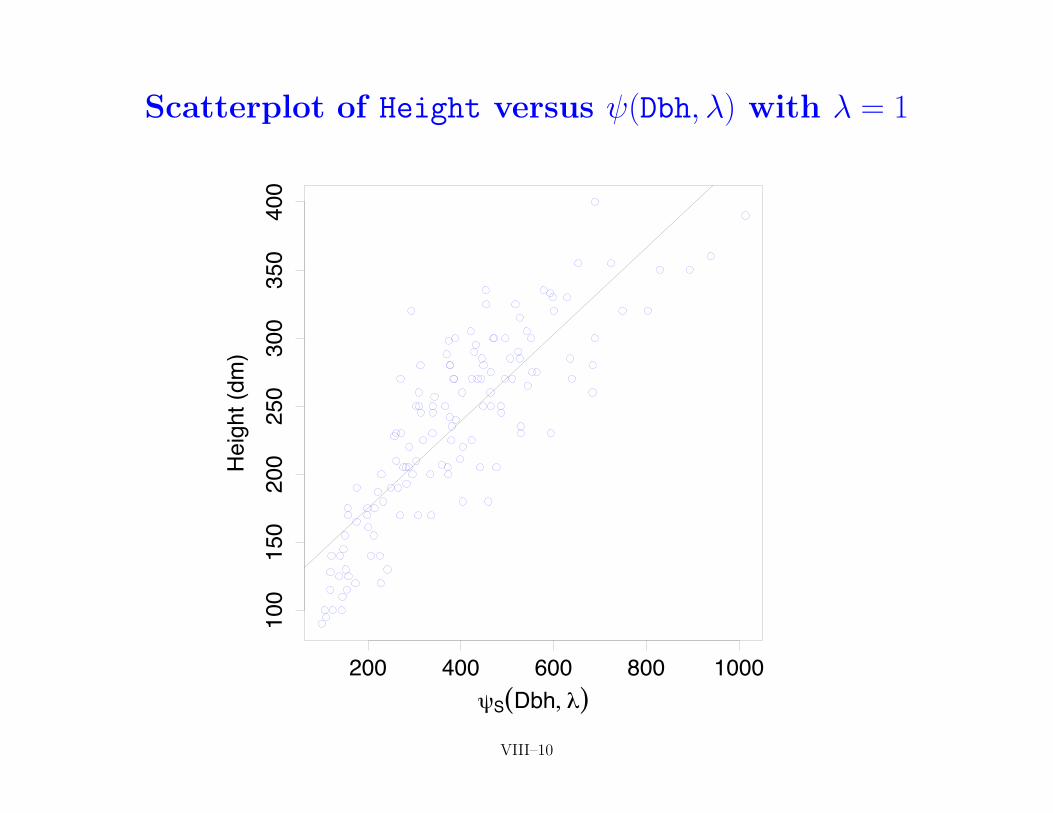
Scatterplot of Height versus (Dbh,�) with � = 1
200 400 600 800 1000
100
150
200
250
300
350
400
sS(Dbh, h)
Hei
ght (
dm)
VIII–10

Scatterplot of Height versus (Dbh,�) with � = 2
0e+00 1e+05 2e+05 3e+05 4e+05 5e+05
100
150
200
250
300
350
400
sS(Dbh, h)
Hei
ght (
dm)
VIII–10
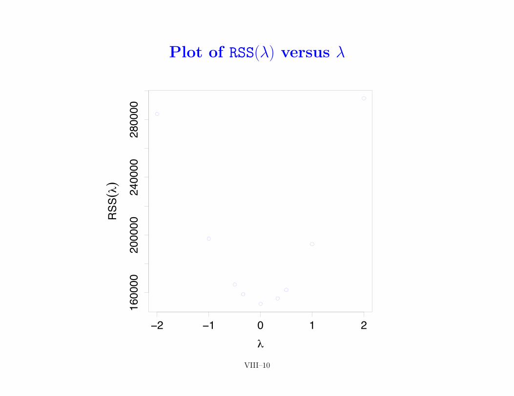
Plot of RSS(�) versus �
−2 −1 0 1 2
160000
200000
240000
280000
h
RSS(h)
VIII–10

Transforming One Regressor: V
• alternative way of displaying transform
� regress yi = Heighti on xi = (Dbhi,�), i = 1, . . . , n,where xi is transformed value of xi = Dbhi
� find min & max values Dbhmin & Dbhmax of Dbhi
� form dense grid of values x⇤j , j = 1, . . . ,m, ranging fromDbhmin to Dbhmax
� compute predicted values y⇤j corresponding to (x⇤j ,�)
� plot y⇤j versus x⇤j on original scatterplot of yi versus xi
ALR–189, 190 VIII–11

Scatterplot of Height versus Dbh with � = �2
200 400 600 800 1000
100
150
200
250
300
350
400
Dbh (mm)
Hei
ght (
dm)
VIII–12

Scatterplot of Height versus Dbh with � = �1
200 400 600 800 1000
100
150
200
250
300
350
400
Dbh (mm)
Hei
ght (
dm)
ALR–190 VIII–12

Scatterplot of Height versus Dbh with � = �1/2
200 400 600 800 1000
100
150
200
250
300
350
400
Dbh (mm)
Hei
ght (
dm)
VIII–12

Scatterplot of Height versus Dbh with � = �1/3
200 400 600 800 1000
100
150
200
250
300
350
400
Dbh (mm)
Hei
ght (
dm)
VIII–12

Scatterplot of Height versus Dbh with � = 0
200 400 600 800 1000
100
150
200
250
300
350
400
Dbh (mm)
Hei
ght (
dm)
ALR–190 VIII–12

Scatterplot of Height versus Dbh with � = 1/3
200 400 600 800 1000
100
150
200
250
300
350
400
Dbh (mm)
Hei
ght (
dm)
VIII–13

Scatterplot of Height versus Dbh with � = 1/2
200 400 600 800 1000
100
150
200
250
300
350
400
Dbh (mm)
Hei
ght (
dm)
VIII–13

Scatterplot of Height versus Dbh with � = 1
200 400 600 800 1000
100
150
200
250
300
350
400
Dbh (mm)
Hei
ght (
dm)
ALR–190 VIII–13

Scatterplot of Height versus Dbh with � = 2
200 400 600 800 1000
100
150
200
250
300
350
400
Dbh (mm)
Hei
ght (
dm)
VIII–13

Scatterplot of Height versus Dbh, � = �1, 0, 1
200 400 600 800 1000
100
150
200
250
300
350
400
Dbh (mm)
Hei
ght (
dm)
ALR–190 VIII–13

Plot Created by R Function invTranPlot
200 400 600 800 1000
100
150
200
250
300
350
400
Dbh
Height
h: 0.05 −1 0 1
ALR–190 VIII–14

Scatterplot for Liquid Copper Example
0.2 0.4 0.6 0.8
300
400
500
600
700
Sulfur
Tension
h: 0.03 −1 0 1
ALR–199, 200 VIII–15

Transforming Response: I
• assuming regressor X has been suitably transformed into eX,now consider transforming response Y
• will consider two methods, the first of which is based on model
E(Y | Y = y) = ↵0 + ↵1 S(y,�),
where Y is fitted value from regression of Y on eX – recall thatY is a linear transformation of eX (note: need to assume Y > 0)
• model is analogous to
E(Y | X = x) = �0 + �1 S(x,�),
so the idea is to use same procedure as we did for selecting eX• leads to creation of inverse fitted value plot of Y versus Y
(also called an inverse response plot)
• let’s look at three examples (using eX = log(X) for first two)
ALR–196, 197 VIII–16

Inverse Fitted Value Plot for Cedar Tree Example
100 150 200 250 300 350 400
100
150
200
250
300
350
Height
Fitte
d he
ight
h: 0.23 −1 0 1
VIII–17

Inverse Fitted Value Plot for Liquid Copper Example
300 400 500 600 700
300
400
500
600
700
Tension
Fitte
d te
nsio
n
h: 0.69 −1 0 1
VIII–18

Inverse Fitted Value Plot for Forbes Example
22 24 26 28 30
2224
2628
30
Pressure
Fitte
d pr
essu
re
h: 0.4 −1 0 1
VIII–19

Transforming Response: II
• 2nd method (called Box–Cox method) makes use of family ofmodified power transformations (note: again we need Y > 0):
M(Y,�) = gm(Y )1�� ⇥ S(Y,�) =
(gm(Y )1�� ⇥ (Y � � 1)/�, � 6= 0
gm(Y )1�� ⇥ log(Y ), � = 0,
where gm(Y ) is geometric mean of untransformed responsesy1, . . . , yn:
gm(Y ) =
0@ nY
i=1
yi
1A
1/n
= exp
0@1
n
nXi=1
log(yi)
1A
� 2nd form is computationally preferable on a computer
• so: what is the rationale for multiplying by geometric mean?
ALR–198, 190, 191 VIII–20

Transforming Response: III
• residual sum of squares function when transforming predictor:
RSSp,S(b0, b1,�) =nX
i=1
[yi � (b0 + b1 S(xi,�))]2
• for each �, measures how well we predict yi’s
• residual sum of squares function when transforming response:
RSSr,S(b0, b1,�) =nX
i=1
[ S(yi,�)� (b0 + b1xi)]2
• for each �, measures how well we predict S(yi,�)’s
• units of S(yi,�) change as � changes, leading to concernsabout comparing ‘apples & oranges’ (because b1 changes unitsimplicitly, not a concern with RSSp,S(b0, b1,�))
ALR–190, 191 VIII–21

Transforming Response: IV
• when � 6= 0, have
M(Y,�) =
2640@ nY
i=1
Yi
1A
1/n375
1��
⇥ Y � � 1
�
• if Y has units of m (meters), thenQn
i=1 Yi has units of mn
• (Qn
i=1 Yi)1/n has units of m; [(
Qni=1 Yi)
1/n]1��, units of m1��
• Y � has units of m�, so M(Y,�) has units of m for all �
• thus: transformed & untransformed responses have same units
ALR–190, 191 VIII–22

Transforming Response: V
• resulting residual sum of squares function, i.e.,
RSSr,M(b0, b1,�) =nX
i=1
[ M(yi,�)� (b0 + b1xi)]2 ,
measured in same units for all �, thus eliminating ‘apples andoranges’ concern
• for fixed �, minimizer of above is OLS estimators �0 and �1from regression of M(yi,�) on xi, resulting in
RSSr,M(�) = RSSr,M(�0, �1,�)
• as before, select � such that RSSr,M(�) is minimized over �
• let’s consider same three examples again (using eX = log(X)for first two)
ALR–198, 190, 191 VIII–23

Scatterplot for Cedar Tree Example
5.0 5.5 6.0 6.5 7.0
100
150
200
250
300
350
400
log(Dbh)
Hei
ght (
dm)
h = 0.6h = −1h = 0h = 1
VIII–24
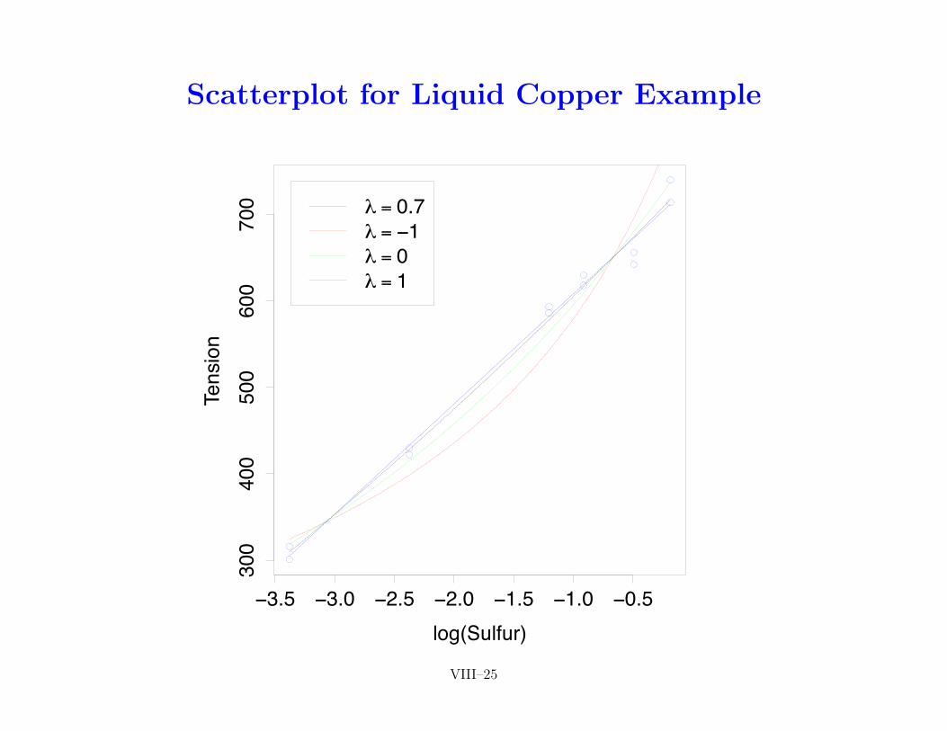
Scatterplot for Liquid Copper Example
−3.5 −3.0 −2.5 −2.0 −1.5 −1.0 −0.5
300
400
500
600
700
log(Sulfur)
Tension
h = 0.7h = −1h = 0h = 1
VIII–25

Scatterplot for Forbes Example
195 200 205 210
2224
2628
30
Boiling point
Pres
sure
h = 0.4h = −1h = 0h = 1
VIII–26

Transforming Response: VI
• display of transforms done as follows:
� regress yi = M(yi,�) on xi, i = 1, . . . , n
� find min & max values xmin & xmax of xi
� form dense grid of values x⇤j , j = 1, . . . ,m, ranging fromxmin to xmax
� compute predicted values y⇤j over dense grid
� plot �1M (y⇤j ,�) versus x⇤j on original scatterplot, where
�1M (Y ⇤,�) =
((1 + �Y ⇤/gm(Y )1��)1/�, � 6= 0
exp(Y ⇤/gm(Y )), � = 0
(note that �1M ( M(Y,�),�) = Y )
VIII–27

Summary of Regressor and Response Transforms
• here is a table showing �’s chosen so far
responseExample regressor 1st method 2nd methodCedar tree 0 0.2 0.6Liquid copper 0 0.7 0.7Forbes 1 0.4 0.4
• �’s chosen by two methods for transforming response disagreefor cedar tree example, but agree for other two examples
• following plots for � = 0, 0.2, 0.6 and 1 for cedar tree examplesuggest that using � = 0 or 0.2 impart some curvature, whereas� = 0.6 or 1 (i.e., no transformation) do not
• going with no transformation is a simple (& reasonable) choice
VIII–28

� = 0 Transformation with Linear & Quadratic Fits
5.0 5.5 6.0 6.5 7.0
4.5
5.0
5.5
6.0
log(Dbh)
log(Height)
VIII–29

� = 0.2 Transformation with Linear & Quadratic Fits
5.0 5.5 6.0 6.5 7.0
2.6
2.8
3.0
3.2
log(Dbh)
Height0.2
VIII–30

� = 0.6 Transformation with Linear & Quadratic Fits
5.0 5.5 6.0 6.5 7.0
1520
2530
35
log(Dbh)
Height0.6
VIII–31

� = 1 Transformation with Linear & Quadratic Fits
5.0 5.5 6.0 6.5 7.0
100
150
200
250
300
350
400
log(Dbh)
Hei
ght (
dm)
ALR–191 VIII–32

Transformations for Multiple Regressors: I
• focusing now on MLR, ‘overall goal is to find transformations inwhich MLR matches the data to a reasonable approximation’(Weisberg, p. 193)
• theoretical arguments (Weisberg, pp. 193–4) suggest we canmake progress towards this goal if regressors in mean functionare all linearly related
• if, through suitable transformations, we arrive at regressors eXthat are approximately pairwise linear, theoretical argumentssay that, under certain conditions (some restrictive!), fittingmean function E(Y | eX = x) = �0x using OLS allows us toidentify unknown function g(·) in more general model
E(Y | eX = x) = g(�0x)
from a scatterplot of yi versus fitted values �0xi
ALR–193, 194 VIII–33

Transformations for Multiple Regressors: II
• overall strategy is thus:
1. transform regressors so that all pairwise scatterplots are ap-proximately linear (don’t worry about scatterplots of Y ver-sus individual regressors)
2. regress Y on transformed regressors eX to get estimates �
3. determine a suitable transform for Y using one of two meth-ods discussed previously (see VIII–16 and VIII–20), leadingto MLR model
E( (Y,�) | eX = x) = ↵0x
• starting point in achieving 1 is study of scatterplot matrix
• quickly leads to realization that achieving 1 can be daunting!
• Weisberg (§8.2) uses Highway data as an illustration
ALR–194, 195, 191 VIII–34

Transformations for Multiple Regressors: III
• goal is to predict response rate (accidents per million vehiclemiles for a particular highway segment) using as regressors
� len, length of highway segment in miles
� adt, average daily tra�c count in thousands
� trks, truck volume as % of total volume
� slim, speed limit
� shld, shoulder width of outer shoulder on roadway
� sigs, number of interchanges with signals per mile
ALR–192 VIII–35

Scatterplot Matrix for Untransformed Highway Data
len
0 30 60 40 55 70 0.0 1.0 2.0
1030
030
60
adt
trks
610
14
4055
70
slim
shld
26
10
10 30
0.0
1.0
2.0
6 10 14 2 6 10
sigs
ALR–193 VIII–36

Enhanced Scatterplot Matrix
len0 30 60 40 55 70 0.0 1.0 2.0
1030
030
60 adt
trks
610
14
4055
70 slim
shld
26
10
10 30
0.0
1.0
2.0
6 10 14 2 6 10
sigs
ALR–193 VIII–37

Enhanced Matrix for Selected Regressors: I
len
0 10 30 50 70
1020
3040
010
3050
70 adt
10 20 30 40 6 8 10 12 14
68
1012
14trks
ALR–193 VIII–38

Enhanced Matrix for Selected Regressors: II
len
40 50 60 70 0.0 1.0 2.0
1020
3040
4050
6070
slim
shld
24
68
10
10 20 30 40
0.0
1.0
2.0
2 4 6 8 10
sigs
ALR–193 VIII–39

Enhanced Matrix for Selected Regressors: III
adt
40 50 60 70 0.0 1.0 2.0
020
4060
4050
6070
slim
shld
24
68
10
0 20 40 60
0.0
1.0
2.0
2 4 6 8 10
sigs
ALR–193 VIII–40

Enhanced Matrix for Selected Regressors: IV
trks
40 50 60 70 0.0 1.0 2.0
68
1012
14
4050
6070
slim
shld
24
68
10
6 8 10 12 14
0.0
1.0
2.0
2 4 6 8 10
sigs
ALR–193 VIII–41

Transformations for Multiple Regressors: IV
• all regressors positive except sigs (# of signaled interchangesper mile), which has some values equal to zero
� can handle sigs by defining new regressor
sigs1 =sigs⇥ len + 1
len(i.e., bump up signal count by 1 in every segment)
• slim (speed limit) doesn’t vary much (most values between 50to 60 mph, with total range being between 40 and 70 mph)
� unlikely any transformation (slim,�) will be e↵ective
• with sigs replaced by sigs1 and with slim left out as a can-didate for transformation, can use R function powerTransformto get initial guesses at suitable transformations (implementa-tion of multivariate extension of Box–Cox due to Velilla)
ALR–192, 195, 196 VIII–42

Transformations for Multiple Regressors: V
• output from powerTransform for Highway data:
Est.Power Std.Err. Lower Bound Upper Boundlen 0.1437 0.2127 -0.2732 0.5607adt 0.0509 0.1206 -0.1854 0.2872trks -0.7028 0.6177 -1.9134 0.5078shld 1.3456 0.3630 0.6341 2.0570sigs1 -0.2408 0.1496 -0.5341 0.0525
Likelihood ratio tests about transformation parametersLRT df pval
LR test, lambda = (0 0 0 0 0) 23.32 5 0.0003LR test, lambda = (1 1 1 1 1) 132.86 5 0.0000LR test, lambda = (0 0 0 1 0) 6.09 5 0.2977
ALR–196 VIII–43

Transformations for Multiple Regressors: VI
• can reject null hypothesis of all log transformations and nullhypothesis of no transformations at all
• cannot reject null hypothesis of log transformation for all re-gressors except shld (shoulder width)
• suggestion for trks is a bit odd: sticking to nearest integer �would lead to choice � = �1 rather than � = 0
• can test feasibility of this modification using testTransform,which yields following output for comparison with � = 0 choice:
LRT df pvalLR test, lambda = (0 0 -1 1 0) 4.34 5 0.5022LR test, lambda = (0 0 0 1 0) 6.09 5 0.2977
• cannot reject either of two stated null hypotheses, so will gowith suggested (0, 0, 0, 1, 0) choice for �’s
ALR–196 VIII–44

Scatterplot Matrix for Transformed Highway Data
loglen
0 2 4 40 55 70 −3 −1 1
1.0
2.5
02
4
logadt
logtrks
1.8
2.2
2.6
4055
70
slim
shld
26
10
1.0 2.5
−3−1
1
1.8 2.2 2.6 2 6 10
logsigs1
ALR–197 VIII–45

Enhanced Scatterplot Matrix
loglen
0 2 4 40 55 70 −3 −1 1
1.0
2.5
02
4 logadt
logtrks
1.8
2.2
2.6
4055
70 slim
shld
26
10
1.0 2.5
−3−1
1
1.8 2.2 2.6 2 6 10
logsigs1
ALR–197 VIII–46

Enhanced Matrix for Selected Regressors: I
loglen
0 1 2 3 4
1.0
1.5
2.0
2.5
3.0
3.5
01
23
4 logadt
1.0 1.5 2.0 2.5 3.0 3.5 1.8 2.0 2.2 2.4 2.6
1.8
2.0
2.2
2.4
2.6logtrks
ALR–193 VIII–47

Enhanced Matrix for Selected Regressors: II
loglen40 50 60 70 −3 −2 −1 0 1
1.0
2.0
3.0
4050
6070
slim
shld
24
68
10
1.0 2.0 3.0
−3−2
−10
1
2 4 6 8 10
logsigs1
ALR–193 VIII–48

Enhanced Matrix for Selected Regressors: III
logadt40 50 60 70 −3 −2 −1 0 1
01
23
4
4050
6070
slim
shld
24
68
10
0 1 2 3 4
−3−2
−10
1
2 4 6 8 10
logsigs1
ALR–193 VIII–49

Enhanced Matrix for Selected Regressors: IV
logtrks40 50 60 70 −3 −2 −1 0 1
1.8
2.2
2.6
4050
6070
slim
shld
24
68
10
1.8 2.2 2.6
−3−2
−10
1
2 4 6 8 10
logsigs1
ALR–193 VIII–50

Transforming Response for Highway Data: I
• with transformations for regressors set, turn attention now totransformation of response using
1. inverse fitted value plot
2. Box–Cox method
• for 1, start by fitting model
E(rate | X) = �0 + �1 ⇥ loglen + �2 ⇥ logadt + �3 ⇥ logtrks
+�4 ⇥ slim + �5 ⇥ shld + �6 ⇥ logsigs1
to obtain fitted values Y for rate
• fit modelE(Y | Y = y) = ↵0 + ↵1 S(y,�)
for various choices of � to create inverse fitted value plot
• following plot suggests log transform might be appropriate
ALR–196 VIII–51

Inverse Fitted Value Plot for Highway Example
2 4 6 8
02
46
8
rate
Fitte
d ra
te
h: 0.18 −1 0 1
ALR–197 VIII–52

Transforming Response for Highway Data: II
• for 2 (Box–Cox method), consider residual sum of squares func-tion
RSSr,M(b,�) =nX
i=1
⇥ M(yi,�)� x0ib
⇤2,
where yi is rate for ith case, and vector xi contains 1 followedby values of loglen, logadt, . . . , logsigs1 for ith case
• for fixed �, minimizer of above is OLS estimator � from regres-sion of M(yi,�) on xi, resulting in
RSSr,M(�) = RSSr,M(�,�)
• as before, select � such that RSSr,M(�) is minimized over �
• following summary plot shows so-called log-likelihood versus�, where log-likelihood is �n
2 log[RSSr,M(�)/n] (suggests logtransform as did inverse fitted value plot)
ALR–198 VIII–53

Summary of Box–Cox Method for Highway Example
−2 −1 0 1 2
−90
−85
−80
−75
−70
h
log−
Like
lihoo
d 95%
ALR–197 VIII–54

Main Points: I
• transformations allow application of SLR and MLR analysisto regressor/response data that, in their original state, are notwell-suited for such analysis
• in SLR, need for transformation suggested by scatterplot of Yversus X with points that aren’t clustered about a line
• useful family of transformations is scaled power transforma-tions:
S(X,�) =
((X� � 1)/�, � 6= 0
log(X), � = 0
(case � = 1 is essentially no transformation at all)
• above requires that regressor X be positive (§8.4 of Weisbergdiscusses a (not entirely satisfactory) modification for handlingdata that can take both positive and negative values)
ALR–185, 189, 198, 199 VIII–55

Main Points: II
• appropriate � is value minimizing residual sum of squares (RSS)of Y regressed on S(X,�)
• once X has been suitably transformed, can use either
1. inverse fitted value plot or
2. Box–Cox method
to select a power transformation suitable for Y > 0 (2ndmethod makes use of a modified power transformation, whichdi↵ers from a scaled power transformation by a normalizingfactor involving the geometric mean of responses yi)
ALR–189, 196, 198 VIII–56

Main Points: III
• in MLR, good to have regressors whose entries in scatterplotmatrix show a linear relationship
• if original regressors don’t have this pattern, transformation ofone or more regressors is called for
• identifying which transformation to apply to which regressorcan be a daunting task
• task can be facilitated by an automatic transformation selectionmethod due to Velilla, which can provide a useful starting pointfor picking suitable transformations (part art/part science!)
ALR–193, 194, 195 VIII–57

Additional Reference
• G.E.P. Box (1979), ‘Robustness in the Strategy of Scientific Model Building,’ in Robustnessin Statistics, edited by R.L. Launer and G.N. Wilkinson, New York: Academic Press,pp. 201–235
VIII–58