Embed Size (px)
Citation preview
Lecture 2
Signal Processing and Dynamic Time Warping
Michael Picheny, Bhuvana Ramabhadran, Stanley F. Chen
IBM T.J. Watson Research CenterYorktown Heights, New York, USA
{picheny,bhuvana,stanchen}@us.ibm.com
17 September 2012
Administrivia
Students are 75% EE, 25% CS.Top three goals:
General understanding of ASR theory.Learn about ASR implementation/practice.Learn about ML/AI/pattern recognition.
Feedback (2+ votes):Signal processing fast/muddy.Hard to hear/speak too fast.Stan shouldn’t read slides.
Thank you for comments!!!
2 / 120
Demo of Web Site
www.ee.columbia.edu/~stanchen/fall12/e6870/
Will provide hardcopies of readings + slides.PDF readings up on web site by Friday before lecture.
Username: speech, password: pythonrulesPDF slides on web site by 8pm day before lecture (usually).
3 / 120
A Word on Programming Languages
Everyone (not including auditors) knows C, C++, or Java.Will support C++ and Java (not as well).Only basic C++ used; will document stuff outside of C.
C++ is the international language of speech recognition.Speed! (Have you heard of Sphinx 4?)Java users will suffer a little in a couple labs.
Why not Matlab?Can implement signal processing algorithms quickly . . .But not as good for later labs.
4 / 120
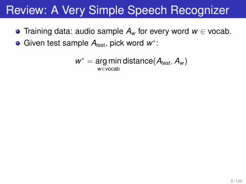
Review: A Very Simple Speech Recognizer
Training data: audio sample Aw for every word w ∈ vocab.Given test sample Atest, pick word w∗:
w∗ = arg minw∈vocab
distance(Atest, Aw)
5 / 120
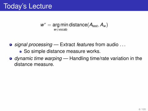
Today’s Lecture
w∗ = arg minw∈vocab
distance(Atest, Aw)
signal processing — Extract features from audio . . .So simple distance measure works.
dynamic time warping — Handling time/rate variation in thedistance measure.
6 / 120
Part I
Signal Processing
7 / 120
Goals of Feature Extraction
Capture essential information for word identification.Make it easy to factor out irrelevant information.
e.g., long-term channel transmission characteristics.Compress information into manageable form.
Figures in this section from [Holmes], [HAH] or [R+J] unless indicatedotherwise.
8 / 120
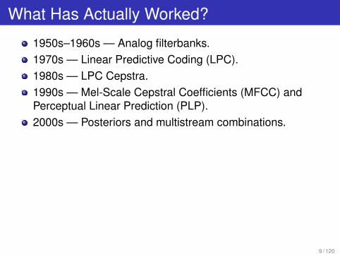
What Has Actually Worked?
1950s–1960s — Analog filterbanks.1970s — Linear Predictive Coding (LPC).1980s — LPC Cepstra.1990s — Mel-Scale Cepstral Coefficients (MFCC) andPerceptual Linear Prediction (PLP).2000s — Posteriors and multistream combinations.
9 / 120
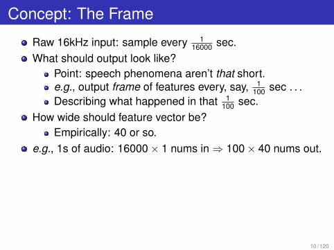
Concept: The Frame
Raw 16kHz input: sample every 116000 sec.
What should output look like?Point: speech phenomena aren’t that short.e.g., output frame of features every, say, 1
100 sec . . .Describing what happened in that 1
100 sec.How wide should feature vector be?
Empirically: 40 or so.e.g., 1s of audio: 16000× 1 nums in ⇒ 100× 40 nums out.
10 / 120
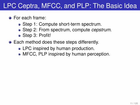
LPC Ceptra, MFCC, and PLP: The Basic Idea
For each frame:Step 1: Compute short-term spectrum.Step 2: From spectrum, compute cepstrum.Step 3: Profit!
Each method does these steps differently.LPC inspired by human production.MFCC, PLP inspired by human perception.
11 / 120
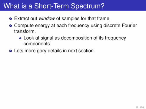
What is a Short-Term Spectrum?
Extract out window of samples for that frame.Compute energy at each frequency using discrete Fouriertransform.
Look at signal as decomposition of its frequencycomponents.
Lots more gory details in next section.
12 / 120
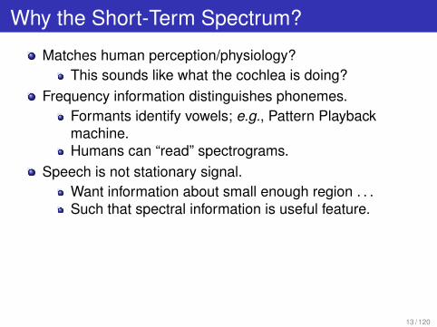
Why the Short-Term Spectrum?
Matches human perception/physiology?This sounds like what the cochlea is doing?
Frequency information distinguishes phonemes.Formants identify vowels; e.g., Pattern Playbackmachine.Humans can “read” spectrograms.
Speech is not stationary signal.Want information about small enough region . . .Such that spectral information is useful feature.
13 / 120
What is a Cepstrum?
(Inverse) Fourier transform of . . .Logarithm of the (magnitude of the) spectrum.Homomorphic transformation
In practice, spectrum is “smoothed” first.e.g., via LPC and/or Mel binning.
14 / 120
What is a Cepstrum?
(Inverse) Fourier transform of . . .Logarithm of the (magnitude of the) spectrum.Homomorphic transformation
In practice, spectrum is “smoothed” first.e.g., via LPC and/or Mel binning.
15 / 120

Why the Cepstrum?
Lets us separate excitation (source; don’t care) . . .From vocal tract resonances (filter; do care).
Vocal tract changes shape slowly with time.Assume fixed properties over small interval (10 ms).Its natural frequencies are formants (resonances).
Low quefrencies correspond to vocal tract.
16 / 120
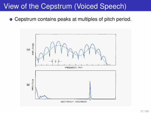
View of the Cepstrum (Voiced Speech)
Cepstrum contains peaks at multiples of pitch period.
17 / 120
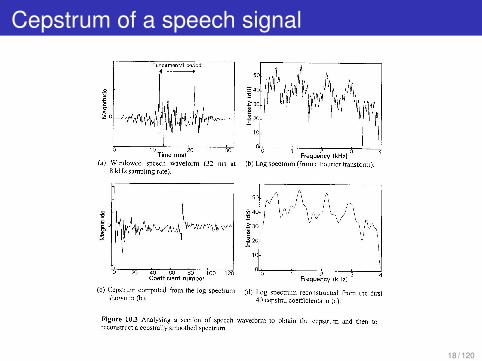
Cepstrum of a speech signal
18 / 120
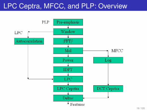
LPC Ceptra, MFCC, and PLP: Overview
19 / 120

Where Are We?
1 The Short-Time Spectrum
2 Scheme 1: LPC
3 Scheme 2: MFCC
4 Scheme 3: PLP
5 Bells and Whistles
6 Discussion20 / 120
The Short-Time Spectrum
Extract out window of N samples for that frame.Compute energy at each frequency using fast Fouriertransform.
Standard algorithm for computing DFT.Complexity N log N; usually take N = 512, 1024 or so.
What’s the problem?The devil is in the details.e.g., frame rate; window length; window shape.
21 / 120
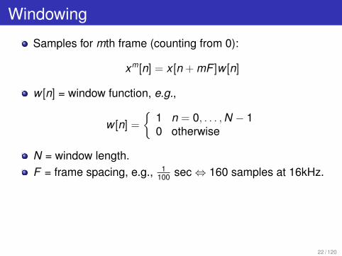
Windowing
Samples for mth frame (counting from 0):
xm[n] = x [n + mF ]w [n]
w [n] = window function, e.g.,
w [n] =
{1 n = 0, . . . , N − 10 otherwise
N = window length.F = frame spacing, e.g., 1
100 sec ⇔ 160 samples at 16kHz.
22 / 120
How to Choose Frame Spacing?
Experiments in speech coding intelligibility suggest that Fshould be around 10 msec (= 1
100 sec).For F > 20 msec, one starts hearing noticeable distortion.Smaller F and no improvement.
The smaller the F , the more the computation.
23 / 120
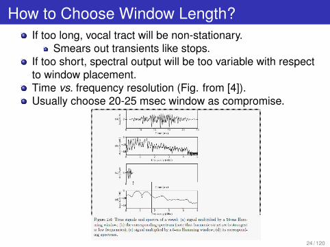
How to Choose Window Length?If too long, vocal tract will be non-stationary.
Smears out transients like stops.If too short, spectral output will be too variable with respectto window placement.Time vs. frequency resolution (Fig. from [4]).Usually choose 20-25 msec window as compromise.
24 / 120
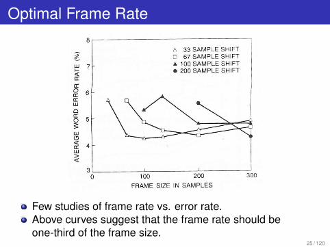
Optimal Frame Rate
Few studies of frame rate vs. error rate.Above curves suggest that the frame rate should beone-third of the frame size.
25 / 120
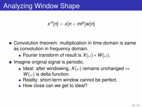
Analyzing Window Shape
xm[n] = x [n + mF ]w [n]
Convolution theorem: multiplication in time domain is sameas convolution in frequency domain.
Fourier transform of result is X (ω) ∗W (ω).Imagine original signal is periodic.
Ideal: after windowing, X (ω) remains unchanged ⇔W (ω) is delta function.Reality: short-term window cannot be perfect.How close can we get to ideal?
26 / 120
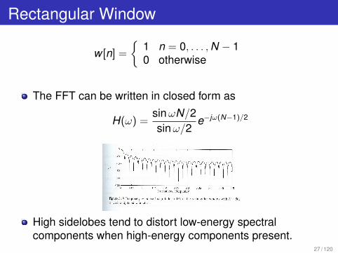
Rectangular Window
w [n] =
{1 n = 0, . . . , N − 10 otherwise
The FFT can be written in closed form as
H(ω) =sin ωN/2sin ω/2
e−jω(N−1)/2
High sidelobes tend to distort low-energy spectralcomponents when high-energy components present.
27 / 120
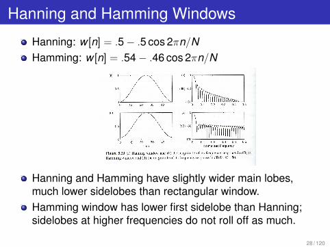
Hanning and Hamming Windows
Hanning: w [n] = .5− .5 cos 2πn/NHamming: w [n] = .54− .46 cos 2πn/N
Hanning and Hamming have slightly wider main lobes,much lower sidelobes than rectangular window.Hamming window has lower first sidelobe than Hanning;sidelobes at higher frequencies do not roll off as much.
28 / 120
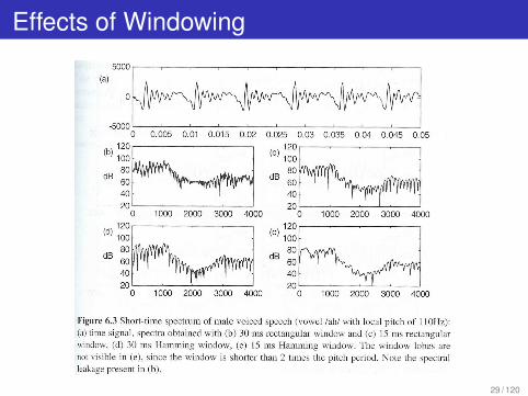
Effects of Windowing
29 / 120
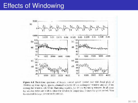
Effects of Windowing
30 / 120
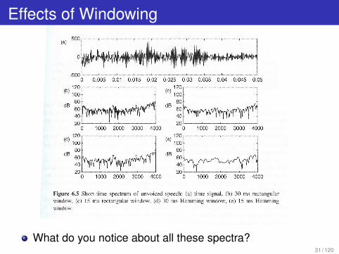
Effects of Windowing
What do you notice about all these spectra?31 / 120

Where Are We?
1 The Short-Time Spectrum
2 Scheme 1: LPC
3 Scheme 2: MFCC
4 Scheme 3: PLP
5 Bells and Whistles
6 Discussion32 / 120
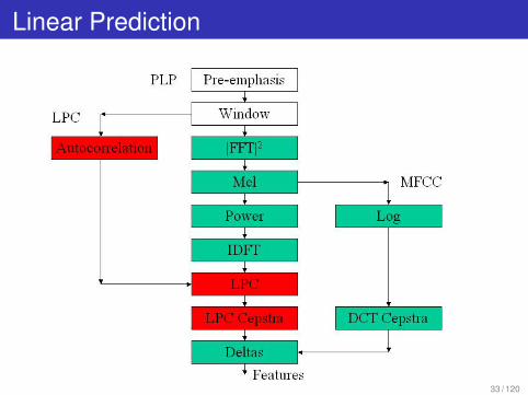
Linear Prediction
33 / 120
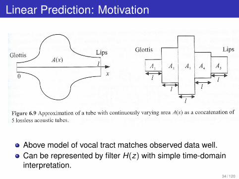
Linear Prediction: Motivation
Above model of vocal tract matches observed data well.Can be represented by filter H(z) with simple time-domaininterpretation.
34 / 120
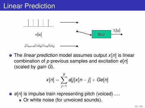
Linear Prediction
The linear prediction model assumes output x [n] is linearcombination of p previous samples and excitation e[n](scaled by gain G).
x [n] =
p∑j=1
a[j ]x [n − j ] + Ge[n]
e[n] is impulse train representing pitch (voiced) . . .Or white noise (for unvoiced sounds).
35 / 120
The General Idea
x [n] =
p∑j=1
a[j ]x [n − j ] + Ge[n]
Given audio signal x [n], solve for a[j ] that . . .Minimizes prediction error.
Ignore e[n] term when solve for a[j ] ⇒ unknown!Assume e[n] will be approximated by prediction error!
The hope:The a[j ] characterize shape of vocal tract.May be good features for identifying sounds?Prediction error is either impulse train or white noise.
36 / 120
Solving the Linear Prediction Equations
Goal: find a[j ] that minimize prediction error:
∞∑n=−∞
(x [n]−p∑
j=1
a[j ]x [n − j ])2
Take derivatives w.r.t. a[i ] and set to 0:
p∑j=1
a[j ]R(|i − j |) = R(i) i = 1, . . . , p
where R(i) is autocorrelation sequence for current windowof samples.Above set of linear equations is Toeplitz and can be solvedusing Levinson-Durbin recursion (O(n2) rather than O(n3)as for general linear equations).
37 / 120
Analyzing Linear Prediction
Recall: Z-Transform is generalization of Fourier transform.The Z-transform of associated filter is:
H(z) =G
1−∑p
j=1 a[j ]z−j
H(z) with z = ejω gives us LPC spectrum.
38 / 120
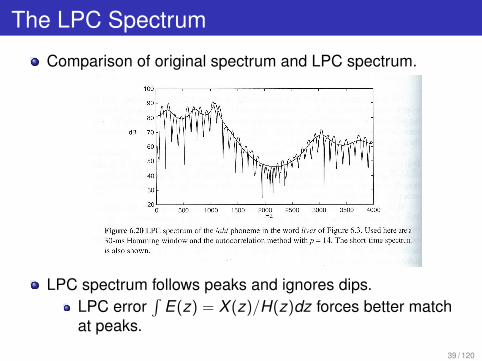
The LPC Spectrum
Comparison of original spectrum and LPC spectrum.
LPC spectrum follows peaks and ignores dips.LPC error
∫E(z) = X (z)/H(z)dz forces better match
at peaks.
39 / 120
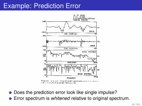
Example: Prediction Error
Does the prediction error look like single impulse?Error spectrum is whitened relative to original spectrum.
40 / 120
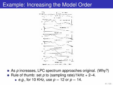
Example: Increasing the Model Order
As p increases, LPC spectrum approaches original. (Why?)Rule of thumb: set p to (sampling rate)/1kHz + 2–4.
e.g., for 10 KHz, use p = 12 or p = 14.41 / 120
Are a[j ] Good Features for ASR?
Nope.Have enormous dynamic range and are very sensitiveto input signal frequencies.Are highly intercorrelated in nonlinear fashion.
Can we derive good features from LP coefficients?Use LPC spectrum? Not compact.Transformation that works best is LPC cepstrum.
42 / 120

The LPC Cepstrum
The complex cepstrum h̃[n] is the inverse DFT of . . .The logarithm of the spectrum.
h̃[n] =1
2π
∫ln H(ω)ejωndω
Using Z-Transform notation:
ln H(z) =∑
h̃[n]z−n
Substituting in H(z) for a LPC filter:
∞∑n=−∞
h̃[n]z−n = ln G − ln(1−p∑
j=1
a[j ]z−j)
43 / 120
The LPC Cepstrum (cont’d)
After some math, we get:
h̃[n] =
0 n < 0
ln G n = 0a[n] +
∑n−1j=1
jn h̃[j ]a[n − j ] 0 < n ≤ p∑n−1
j=n−pjn h̃[j ]a[n − j ] n > p
i.e., given a[j ], easy to compute LPC cepstrum.In practice, 12–20 cepstrum coefficients are adequate forASR (depending upon the sampling rate and whether youare doing LPC or PLP).
44 / 120
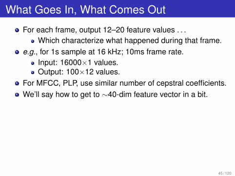
What Goes In, What Comes Out
For each frame, output 12–20 feature values . . .Which characterize what happened during that frame.
e.g., for 1s sample at 16 kHz; 10ms frame rate.Input: 16000×1 values.Output: 100×12 values.
For MFCC, PLP, use similar number of cepstral coefficients.We’ll say how to get to ∼40-dim feature vector in a bit.
45 / 120
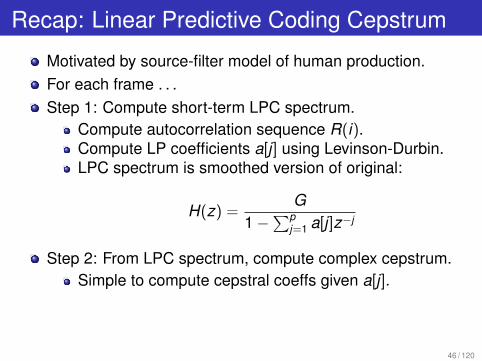
Recap: Linear Predictive Coding Cepstrum
Motivated by source-filter model of human production.For each frame . . .Step 1: Compute short-term LPC spectrum.
Compute autocorrelation sequence R(i).Compute LP coefficients a[j ] using Levinson-Durbin.LPC spectrum is smoothed version of original:
H(z) =G
1−∑p
j=1 a[j ]z−j
Step 2: From LPC spectrum, compute complex cepstrum.Simple to compute cepstral coeffs given a[j ].
46 / 120

Where Are We?
1 The Short-Time Spectrum
2 Scheme 1: LPC
3 Scheme 2: MFCC
4 Scheme 3: PLP
5 Bells and Whistles
6 Discussion47 / 120
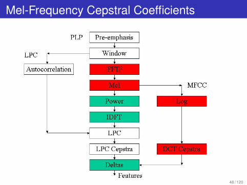
Mel-Frequency Cepstral Coefficients
48 / 120
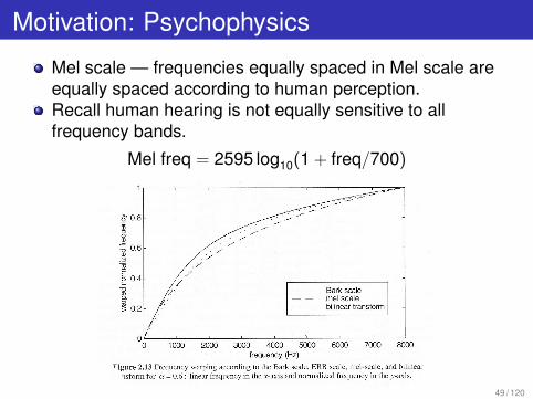
Motivation: Psychophysics
Mel scale — frequencies equally spaced in Mel scale areequally spaced according to human perception.Recall human hearing is not equally sensitive to allfrequency bands.
Mel freq = 2595 log10(1 + freq/700)
49 / 120
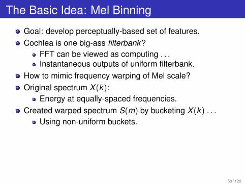
The Basic Idea: Mel Binning
Goal: develop perceptually-based set of features.Cochlea is one big-ass filterbank?
FFT can be viewed as computing . . .Instantaneous outputs of uniform filterbank.
How to mimic frequency warping of Mel scale?Original spectrum X (k):
Energy at equally-spaced frequencies.Created warped spectrum S(m) by bucketing X (k) . . .
Using non-uniform buckets.
50 / 120
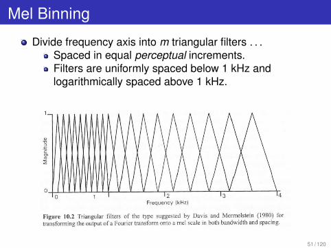
Mel Binning
Divide frequency axis into m triangular filters . . .Spaced in equal perceptual increments.Filters are uniformly spaced below 1 kHz andlogarithmically spaced above 1 kHz.
51 / 120

Why Triangular Filters?
Crude approximation to shape of tuning curves . . .Of nerve fibers in auditory system.
52 / 120
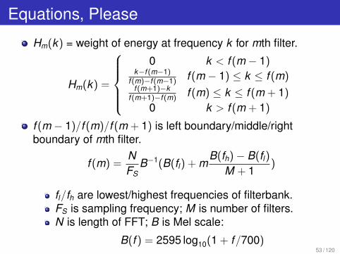
Equations, Please
Hm(k) = weight of energy at frequency k for mth filter.
Hm(k) =
0 k < f (m − 1)
k−f (m−1)f (m)−f (m−1)
f (m − 1) ≤ k ≤ f (m)f (m+1)−k
f (m+1)−f (m)f (m) ≤ k ≤ f (m + 1)
0 k > f (m + 1)
f (m − 1)/f (m)/f (m + 1) is left boundary/middle/rightboundary of mth filter.
f (m) =NFS
B−1(B(fl) + mB(fh)− B(fl)
M + 1)
fl/fh are lowest/highest frequencies of filterbank.FS is sampling frequency; M is number of filters.N is length of FFT; B is Mel scale:
B(f ) = 2595 log10(1 + f/700)53 / 120
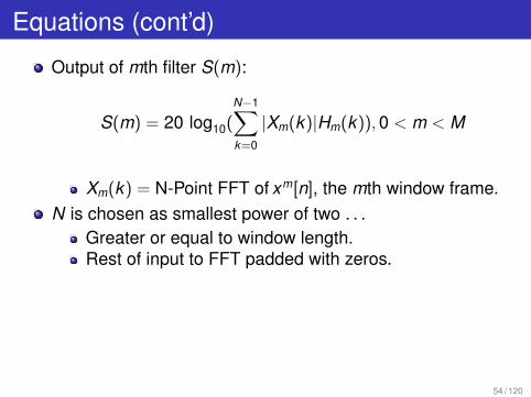
Equations (cont’d)
Output of mth filter S(m):
S(m) = 20 log10(N−1∑k=0
|Xm(k)|Hm(k)), 0 < m < M
Xm(k) = N-Point FFT of xm[n], the mth window frame.N is chosen as smallest power of two . . .
Greater or equal to window length.Rest of input to FFT padded with zeros.
54 / 120
The Mel Frequency Cepstrum
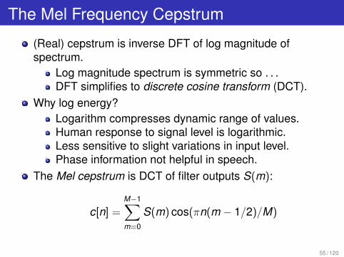
(Real) cepstrum is inverse DFT of log magnitude ofspectrum.
Log magnitude spectrum is symmetric so . . .DFT simplifies to discrete cosine transform (DCT).
Why log energy?Logarithm compresses dynamic range of values.Human response to signal level is logarithmic.Less sensitive to slight variations in input level.Phase information not helpful in speech.
The Mel cepstrum is DCT of filter outputs S(m):
c[n] =M−1∑m=0
S(m) cos(πn(m − 1/2)/M)
55 / 120
The Discrete Cosine Transform
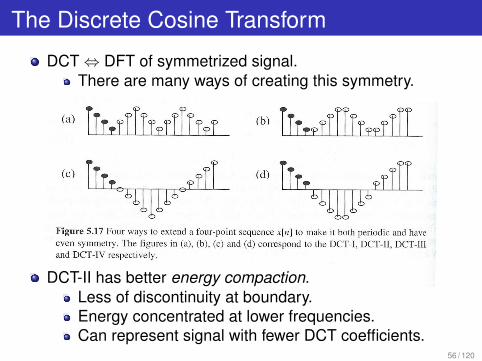
DCT ⇔ DFT of symmetrized signal.There are many ways of creating this symmetry.
DCT-II has better energy compaction.Less of discontinuity at boundary.Energy concentrated at lower frequencies.Can represent signal with fewer DCT coefficients.
56 / 120
Mel Frequency Cepstral Coefficients
Motivated by human perception.For each frame . . .Step 1: Compute frequency-warped spectrum S(m).
Take original spectrum and apply Mel binning.Step 2: Compute cepstrum using DCT . . .
From warped spectrum S(m).
57 / 120

Where Are We?
1 The Short-Time Spectrum
2 Scheme 1: LPC
3 Scheme 2: MFCC
4 Scheme 3: PLP
5 Bells and Whistles
6 Discussion58 / 120
Perceptual Linear Prediction
59 / 120
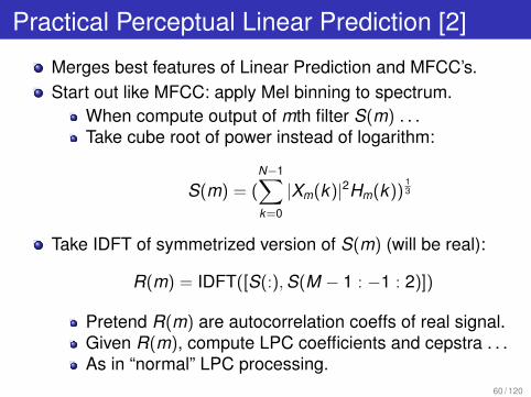
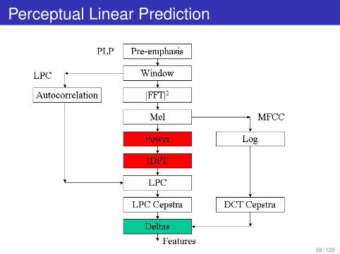
Practical Perceptual Linear Prediction [2]
Merges best features of Linear Prediction and MFCC’s.Start out like MFCC: apply Mel binning to spectrum.
When compute output of mth filter S(m) . . .Take cube root of power instead of logarithm:
S(m) = (N−1∑k=0
|Xm(k)|2Hm(k))13
Take IDFT of symmetrized version of S(m) (will be real):
R(m) = IDFT([S(:), S(M − 1 : −1 : 2)])
Pretend R(m) are autocorrelation coeffs of real signal.Given R(m), compute LPC coefficients and cepstra . . .As in “normal” LPC processing.
60 / 120
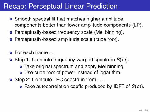
Recap: Perceptual Linear Prediction
Smooth spectral fit that matches higher amplitudecomponents better than lower amplitude components (LP).Perceptually-based frequency scale (Mel binning).Perceptually-based amplitude scale (cube root).
For each frame . . .Step 1: Compute frequency-warped spectrum S(m).
Take original spectrum and apply Mel binning.Use cube root of power instead of logarithm.
Step 2: Compute LPC cepstrum from . . .Fake autocorrelation coeffs produced by IDFT of S(m).
61 / 120

Where Are We?
1 The Short-Time Spectrum
2 Scheme 1: LPC
3 Scheme 2: MFCC
4 Scheme 3: PLP
5 Bells and Whistles
6 Discussion62 / 120
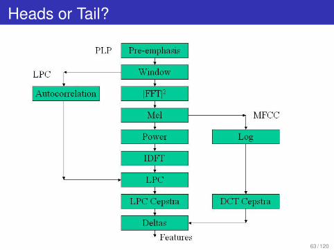
Heads or Tail?
63 / 120
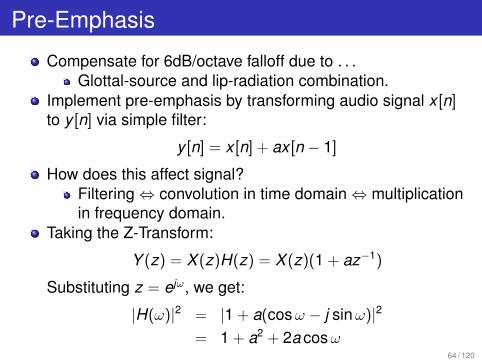
Pre-Emphasis
Compensate for 6dB/octave falloff due to . . .Glottal-source and lip-radiation combination.
Implement pre-emphasis by transforming audio signal x [n]to y [n] via simple filter:
y [n] = x [n] + ax [n − 1]
How does this affect signal?Filtering ⇔ convolution in time domain ⇔ multiplicationin frequency domain.
Taking the Z-Transform:
Y (z) = X (z)H(z) = X (z)(1 + az−1)
Substituting z = ejω, we get:
|H(ω)|2 = |1 + a(cos ω − j sin ω)|2
= 1 + a2 + 2a cos ω64 / 120
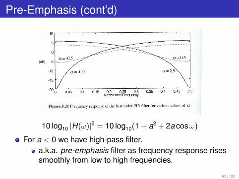
Pre-Emphasis (cont’d)
10 log10 |H(ω)|2 = 10 log10(1 + a2 + 2a cos ω)
For a < 0 we have high-pass filter.a.k.a. pre-emphasis filter as frequency response risessmoothly from low to high frequencies.
65 / 120
Properties
Improves LPC estimates (works better with “flatter” spectra).Reduces or eliminates “DC” (constant) offsets.Mimics equal-loudness contours.
Higher frequency sounds appear “louder” than lowfrequency sounds given same amplitude.
66 / 120
Deltas and Double Deltas
Story so far: use 12–20 cepstral coeffs as features to . . .Describe what happened in current 10–20 msecwindow.
Problem: dynamic characteristics of sounds are important!e.g., stop closures and releases; formant transitions.e.g., phenomena that are longer than 20 msec.
One idea: directly model the trajectories of features.Simpler idea: deltas and double deltas.
67 / 120
The Basic Idea
Augment original “static” feature vector . . .With 1st and 2nd derivatives of each value w.r.t. time.
Deltas: if yt is feature vector at time t , take:
∆yt = yt+D − yt−D
and create new feature vector
y ′t = (yt , ∆yt)
Doubles size of feature vector.D is usually one or two frames.Simple, but can help significantly.
68 / 120
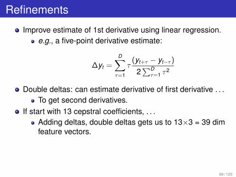
Refinements
Improve estimate of 1st derivative using linear regression.e.g., a five-point derivative estimate:
∆yt =D∑
τ=1
τ(yt+τ − yt−τ )
2∑D
τ=1 τ 2
Double deltas: can estimate derivative of first derivative . . .To get second derivatives.
If start with 13 cepstral coefficients, . . .Adding deltas, double deltas gets us to 13×3 = 39 dimfeature vectors.
69 / 120

Where Are We?
1 The Short-Time Spectrum
2 Scheme 1: LPC
3 Scheme 2: MFCC
4 Scheme 3: PLP
5 Bells and Whistles
6 Discussion70 / 120
Did We Satisfy Our Original Goals?
Capture essential information for word identification.Make it easy to factor out irrelevant information.
e.g., long-term channel transmission characteristics.Compress information into manageable form.Discuss.
71 / 120
What Feature Representation Works Best?
Literature on front ends is weak?Good early paper by Davis and Mermelstein [1]:
52 different CVC words.2 (!) male speakers.676 tokens in all.
Compared these methods for generating feature vectors:MFCC.LFCC.LPCC.LPC+Itakura metric.LPC Reflection coefficients.
72 / 120
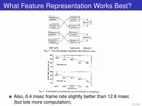
What Feature Representation Works Best?
Also, 6.4 msec frame rate slightly better than 12.8 msec(but lots more computation).
73 / 120
How Things Stand Today
No one uses LPC cepstra any more?Experiments comparing PLP and MFCC are mixed.
Which is better may depend on task.General belief: PLP is usually slightly better.It’s always safe to use MFCC.(Can get some improvement by combining systems?)
74 / 120
Who Made This Stuff Up?
No offense, but this all seems like a big hack.The vocal tract, like the Internet, is series of tubes!? (LPC)“Quefrencies” are best way to identify sounds?
Is there intuitive interpretation of quefrency . . .Computed from Mel spectrum?
That PLP pipeline is one ugly duck.
75 / 120
Points
People have tried hundreds, if not thousands, of methods.MFCC, PLP are what worked best (or at least as well).
What about more data-driven/less knowledge-driven?Instead of hardcoding ideas from speechproduction/perception . . .Try to automatically learn transformation from data?Hasn’t helped yet.
How much audio processing is hardwired in humans?
76 / 120
What About Using Even More Knowledge?
Articulatory features.Neural firing rate models.Formant frequencies.Pitch (except for tonal languages such as Mandarin).Hasn’t helped yet over dumb methods.
Can’t guess hidden values (e.g., formants) well?Some features good for some sounds but not others?Dumb methods automatically learn some of this?
77 / 120
This Isn’t The Whole Story (By a Long Shot)
MFCC/PLP are only starting point for acoustic features!In state-of-the-art systems, do many additionaltransformations on top.
LDA (maximize class separation).Vocal tract normalization.Speaker adaptive transforms.Discriminative transforms.
We’ll talk about this stuff in Lecture 9 (Adaptation).
78 / 120
Hot Topic: Neural Network Bottleneck Feats
Step 1: Build a “conventional” ASR system.Use this to guess (CD) phone identity for each frame.
Step 2: Use this data to train NN that guesses phoneidentity from (conventional) acoustic features.
Use NN with narrow hidden layer, e.g., 40 hidden units.Force NN to try to encode all relevant info about inputin bottleneck layer.
Use hidden unit activations in bottleneck layer as features.Append to or replace original features.
Will be covered more in Lecture 12 (Deep Belief networks).
79 / 120
References
S. Davis and P. Mermelstein, “Comparison of ParametricRepresentations for Monosyllabic Word Recognition inContinuously Spoken Sentences”, IEEE Trans. on Acoustics,Speech, and Signal Processing, 28(4), pp. 357–366, 1980.
H. Hermansky, “Perceptual Linear Predictive Analysis ofSpeech”, J. Acoust. Soc. Am., 87(4), pp. 1738–1752, 1990.
H. Hermansky, D. Ellis and S. Sharma, “Tandemconnectionist feature extraction for conventional HMMsystems”, in Proc. ICASSP 2000, Istanbul, Turkey, June2000.
L. Deng and D. O’Shaughnessy, Speech Processing: ADynamic and Optimization-Oriented Approach, MarcelDekker Inc., 2003.
80 / 120
Part II
Dynamic Time Warping
81 / 120
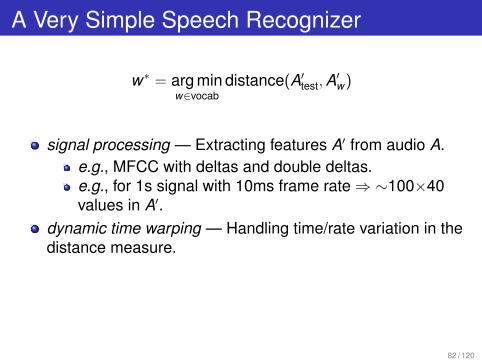
A Very Simple Speech Recognizer
w∗ = arg minw∈vocab
distance(A′test, A′w)
signal processing — Extracting features A′ from audio A.e.g., MFCC with deltas and double deltas.e.g., for 1s signal with 10ms frame rate ⇒ ∼100×40values in A′.
dynamic time warping — Handling time/rate variation in thedistance measure.
82 / 120
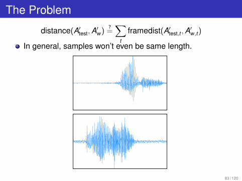
The Problem
distance(A′test, A′w)?=
∑t
framedist(A′test,t , A′w ,t)
In general, samples won’t even be same length.
83 / 120
Problem Formulation
Have two audio samples; convert to feature vectors.Each xt , yt is ∼40-dim vector, say.
X = (x1, x2, . . . , xTx )
Y = (y1, y2, . . . , yTy )
Compute distance(X , Y ).
84 / 120
Linear Time Normalization
Idea: omit/duplicate frames uniformly in Y . . .So same length as X .
distance(X , Y ) =Tx∑
t=1
framedist(xt , yt× Ty
Tx
)
85 / 120
What’s the Problem?
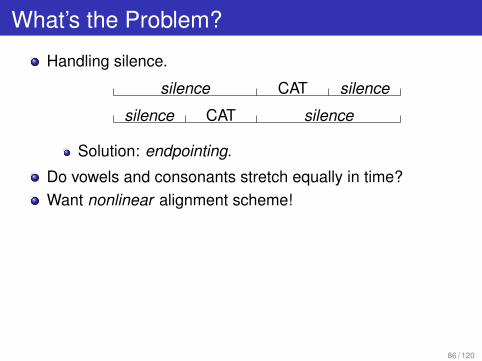
Handling silence.
silence CAT silence
silence CAT silence
Solution: endpointing.
Do vowels and consonants stretch equally in time?Want nonlinear alignment scheme!
86 / 120
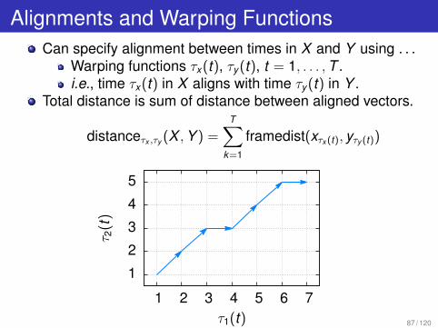
Alignments and Warping FunctionsCan specify alignment between times in X and Y using . . .
Warping functions τx(t), τy(t), t = 1, . . . , T .i.e., time τx(t) in X aligns with time τy(t) in Y .
Total distance is sum of distance between aligned vectors.
distanceτx ,τy (X , Y ) =T∑
k=1
framedist(xτx (t), yτy (t))
1
2
3
4
5
1 2 3 4 5 6 7
τ 2(t
)
τ1(t) 87 / 120
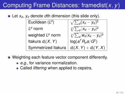
Computing Frame Distances: framedist(x , y)
Let xd , yd denote d th dimension (this slide only).Euclidean (L2)
√∑d(xd − yd)2
Lp norm p√∑
d |xd − yd |p
weighted Lp norm p√∑
d wd |xd − yd |p
Itakura dI(X , Y ) log(aT Rpa/G2)
Symmetrized Itakura dI(X , Y ) + dI(Y , X )
Weighting each feature vector component differently.e.g., for variance normalization.Called liftering when applied to cepstra.
88 / 120
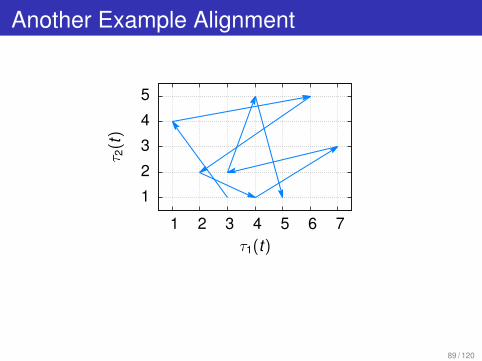
Another Example Alignment
1
2
3
4
5
1 2 3 4 5 6 7
τ 2(t
)
τ1(t)
89 / 120
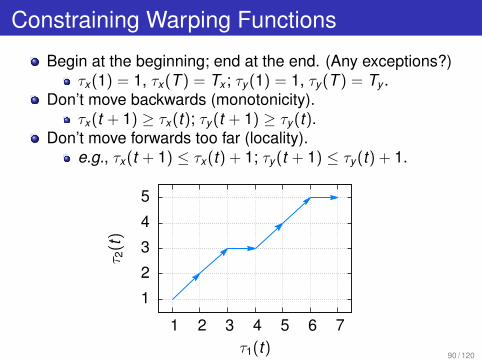
Constraining Warping Functions
Begin at the beginning; end at the end. (Any exceptions?)τx(1) = 1, τx(T ) = Tx ; τy(1) = 1, τy(T ) = Ty .
Don’t move backwards (monotonicity).τx(t + 1) ≥ τx(t); τy(t + 1) ≥ τy(t).
Don’t move forwards too far (locality).e.g., τx(t + 1) ≤ τx(t) + 1; τy(t + 1) ≤ τy(t) + 1.
1
2
3
4
5
1 2 3 4 5 6 7
τ 2(t
)
τ1(t) 90 / 120
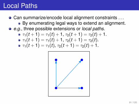
Local Paths
Can summarize/encode local alignment constraints . . .By enumerating legal ways to extend an alignment.
e.g., three possible extensions or local paths.τ1(t + 1) = τ1(t) + 1, τ2(t + 1) = τ2(t) + 1.τ1(t + 1) = τ1(t) + 1, τ2(t + 1) = τ2(t).τ1(t + 1) = τ1(t), τ2(t + 1) = τ2(t) + 1.
91 / 120
Which Alignment?
Given alignment, easy to compute distance:
distanceτx ,τy (X , Y ) =T∑
t=1
framedist(xτx (t), yτy (t))
Lots of possible alignments given X , Y .Which one to use to calculate distance(X , Y )?The best one!
distance(X , Y ) = minvalid τx , τy
{distanceτx ,τy (X , Y )
}
92 / 120
Which Alignment?
distance(X , Y ) = minvalid τx , τy
{distanceτx ,τy (X , Y )
}
Hey, there are many, many possible τx , τy .Exponentially many in Tx and Ty , in fact.
How in blazes are we going to compute this?
93 / 120

Where Are We?
1 Dynamic Programming
2 Discussion
94 / 120
Wake Up!
One of few things you should remember from course.Will be used in many lectures.
If need to find best element in exponential space . . .Rule of thumb: the answer is dynamic programming . . .Or not solvable exactly in polynomial time.
95 / 120
Dynamic Programming
Solve problem by caching subproblem solutions . . .Rather than recomputing them.
Why the mysterious name?The inventor (Richard Bellman) was trying to hide . . .What he was working on from his boss.
For our purposes, we focus on shortest path problems.
96 / 120
Case Study
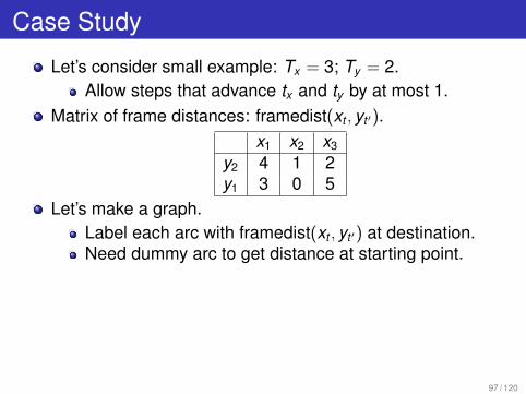
Let’s consider small example: Tx = 3; Ty = 2.Allow steps that advance tx and ty by at most 1.
Matrix of frame distances: framedist(xt , yt ′).x1 x2 x3
y2 4 1 2y1 3 0 5
Let’s make a graph.Label each arc with framedist(xt , yt ′) at destination.Need dummy arc to get distance at starting point.
97 / 120
Case Study
1
2
1 2 3
3
4 1
0
1 2
5
1 2
2
A
B
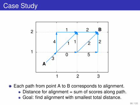
Each path from point A to B corresponds to alignment.Distance for alignment = sum of scores along path.Goal: find alignment with smallest total distance.
98 / 120
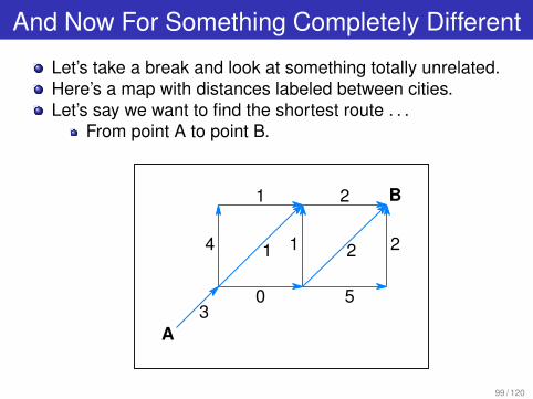
And Now For Something Completely Different
Let’s take a break and look at something totally unrelated.Here’s a map with distances labeled between cities.Let’s say we want to find the shortest route . . .
From point A to point B.
3
4 1
0
1 2
5
1 2
2
A
B
99 / 120
Wait a Second!
I’m having déjà vu!In fact, length of shortest route in 2nd problem . . .
Is same as distance for best alignment in 1st problem.i.e., problem of finding best alignment is equivalent to . . .Single-pair shortest path problem for . . .
Directed acyclic graphs.Has well-known dynamic programming solution.
Will come up again for HMM’s, finite-state machines.
100 / 120
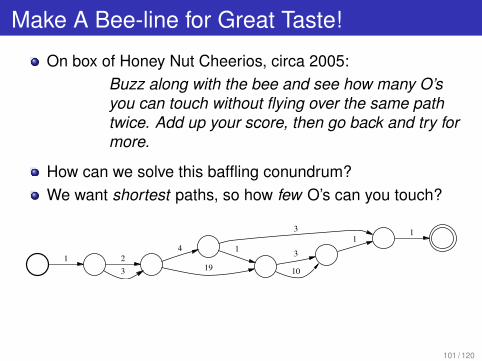
Make A Bee-line for Great Taste!
On box of Honey Nut Cheerios, circa 2005:Buzz along with the bee and see how many O’syou can touch without flying over the same pathtwice. Add up your score, then go back and try formore.
How can we solve this baffling conundrum?We want shortest paths, so how few O’s can you touch?
1 23
4
19
1
3
3
10
11
101 / 120
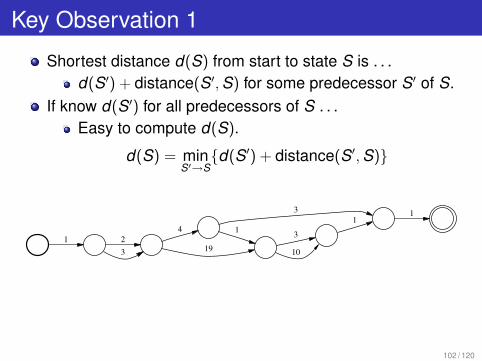
Key Observation 1
Shortest distance d(S) from start to state S is . . .d(S′) + distance(S′, S) for some predecessor S′ of S.
If know d(S′) for all predecessors of S . . .Easy to compute d(S).
d(S) = minS′→S
{d(S′) + distance(S′, S)}
1 23
4
19
1
3
3
10
11
102 / 120
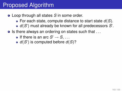
Proposed Algorithm
Loop through all states S in some order.For each state, compute distance to start state d(S).d(S′) must already be known for all predecessors S′.
Is there always an ordering on states such that . . .If there is an arc S′ → S, . . .d(S′) is computed before d(S)?
103 / 120
Key Observation 2
For all acyclic graphs, there is a topological sorting . . .Such that all arcs go from earlier to later states.
In many cases, topological sorting is obvious by inspection.Otherwise, can be computed in time O(states + arcs).
104 / 120
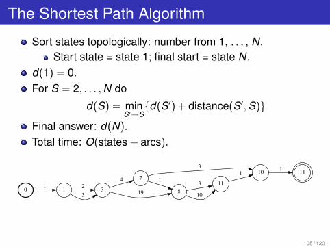
The Shortest Path Algorithm
Sort states topologically: number from 1, . . . , N.Start state = state 1; final start = state N.
d(1) = 0.For S = 2, . . . , N do
d(S) = minS′→S
{d(S′) + distance(S′, S)}
Final answer: d(N).Total time: O(states + arcs).
0 11 323
74
819
110
3
113
10
1111
105 / 120
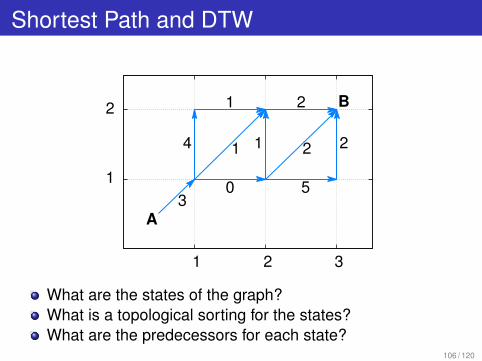
Shortest Path and DTW
1
2
1 2 3
3
4 1
0
1 2
5
1 2
2
A
B
What are the states of the graph?What is a topological sorting for the states?What are the predecessors for each state?
106 / 120
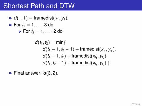
Shortest Path and DTW
d(1, 1) = framedist(x1, y1).For t1 = 1, . . . , 3 do.
For t2 = 1, . . . , 2 do.
d(t1, t2) = min{d(t1 − 1, t2 − 1) + framedist(xt1 , yt2),
d(t1 − 1, t2) + framedist(xt1 , yt2),
d(t1, t2 − 1) + framedist(xt1 , yt2) }
Final answer: d(3, 2).
107 / 120
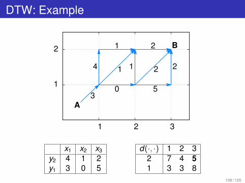
DTW: Example
1
2
1 2 3
3
4 1
0
1 2
5
1 2
2
A
B
x1 x2 x3
y2 4 1 2y1 3 0 5
d(·, ·) 1 2 32 7 4 51 3 3 8
108 / 120

Where Are We?
1 Dynamic Programming
2 Discussion
109 / 120
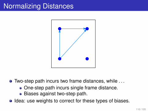
Normalizing Distances
Two-step path incurs two frame distances, while . . .One-step path incurs single frame distance.Biases against two-step path.
Idea: use weights to correct for these types of biases.
110 / 120
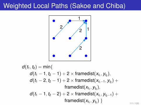
Weighted Local Paths (Sakoe and Chiba)
2
1
2
2
1
d(t1, t2) = min{d(t1 − 1, t2 − 1) + 2× framedist(xt1 , yt2),
d(t1 − 2, t2 − 1) + 2× framedist(xt1−1, yt2) +
framedist(xt1 , yt2),
d(t1 − 1, t2 − 2) + 2× framedist(xt1 , yt2−1) +
framedist(xt1 , yt2) } 111 / 120
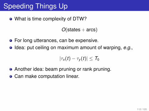
Speeding Things Up
What is time complexity of DTW?
O(states + arcs)
For long utterances, can be expensive.Idea: put ceiling on maximum amount of warping, e.g.,
|τx(t)− τy(t)| ≤ T0
Another idea: beam pruning or rank pruning.Can make computation linear.
112 / 120
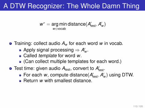
A DTW Recognizer: The Whole Damn Thing
w∗ = arg minw∈vocab
distance(A′test, A′w)
Training: collect audio Aw for each word w in vocab.Apply signal processing ⇒ A′w .Called template for word w .(Can collect multiple templates for each word.)
Test time: given audio Atest, convert to A′test.For each w , compute distance(A′test, A′w) using DTW.Return w with smallest distance.
113 / 120
Recap
DTW is effective for computing distance between signals . . .Using nonlinear time alignment.
Ad hoc selection of frame distance and local paths.Finds best path in exponential space in quadratic time . . .
Using dynamic programming.Signal processing, DTW: all you need for simple ASR.
e.g., old-school cell phone name dialer.
114 / 120
Back to the Future
Some recent work has revisited DTW.Can extend algorithm to connected speech.
Word models (as opposed to phonetic models).Don’t average word instances together; keep separate!Can model longer-distance acoustic dependencies . . .
As compared to conventional GMM/HMM systems.Hasn’t gone anywhere yet.
115 / 120
References
R. Bellman, “Eye of the Hurricane”. World ScientificPublishing Company, Singapore, 1984.
H. Sakoe and S. Chiba, “Dynamic Programming AlgorithmOptimization for Spoken Word Recognition”, IEEE Trans. onAcoustics Speech and Signal Processing, vol. ASSP-26, pp.43–45, Feb. 1978.
116 / 120

Part III
Epilogue
117 / 120
Lab 1
Handed out today; due Wednesday, Oct. 3, 6pm.Write parts of DTW recognizer and run experiments.
Write most of MFCC front end (except for FFT).Optional: write DTW.Optional: try to improve baseline MFCC front end.
118 / 120
The Road Ahead
DTW doesn’t scale: linear in number of templates.10 word voc ⇒ 100k words?1 training sample per word ⇒ 100?
How to deal?Lecture 3: Gaussian mixture models.Lecture 4: Hidden Markov models.
119 / 120
Course Feedback
1 Was this lecture mostly clear or unclear? What was themuddiest topic?
2 Other feedback (pace, content, atmosphere)?
120 / 120