Lecture 19:Shortest Paths

Shang-Hua Teng

Weighted Directed Graphs• Weight on edges for distance

JFK

BOS

MIA

ORD

LAXDFW

SFO

v2

v1v3

v4

v5

v6

v7

400

2500

1000

1800800900

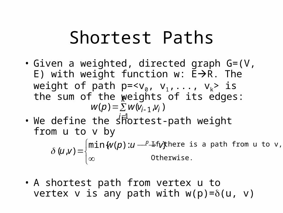
Shortest Paths• Given a weighted, directed graph G=(V, E) with

weight function w: ER. The weight of path p=<v0, v1,..., vk> is the sum of the weights of its edges:

• We define the shortest-path weight from u to v by

• A shortest path from vertex u to vertex v is any path with w(p)=(u, v)

k

iii vvwpw

11 ),()(

}:)(min{

),(

vupw

vup

If there is a path from u to v,

Otherwise.

Variants of Shortest Path Problem• Single-source shortest paths problem

– Finds all the shortest path of vertices reachable from a single source vertex s

• Single-destination shortest-path problem– By reversing the direction of each edge in the graph, we can

reduce this problem to a single-source problem

• Single-pair shortest-path problem– No algorithm for this problem are known that run

asymptotically faster than the best single-source algorithm in the worst case

• All-pairs shortest-path problem

Applications of Shortest Path• Every where!!!

– Driving (GPS)– Internet: network routing– Flying: Airline route– Resource allocation– VLSI design: wire routing– Computer Games– Mapquest, Yahoo map program

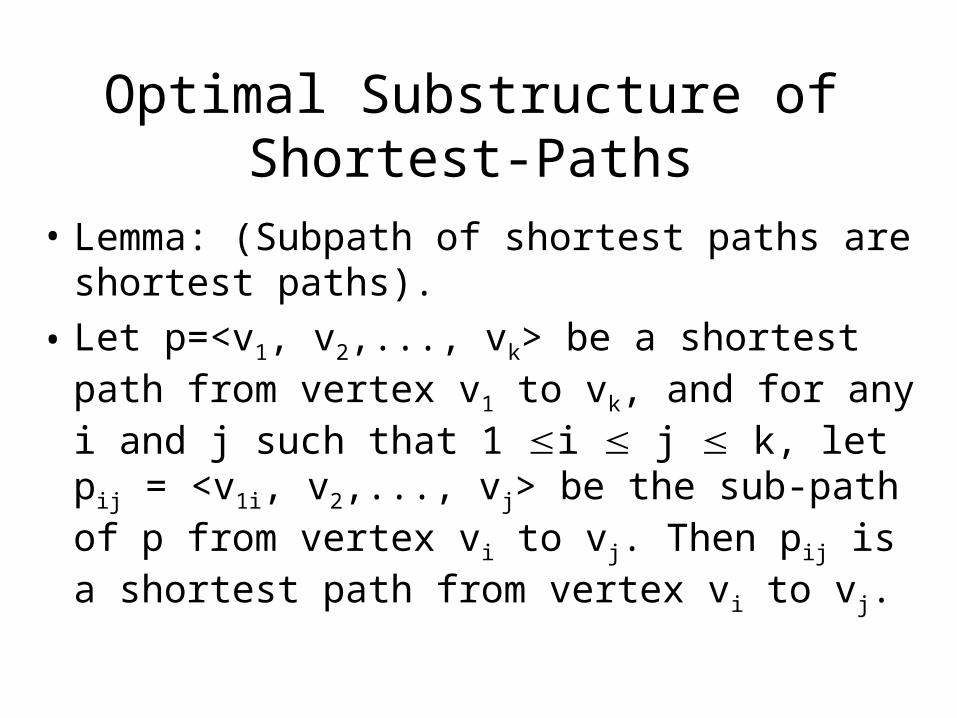
Optimal Substructure of Shortest-Paths

• Lemma: (Subpath of shortest paths are shortest paths).

• Let p=<v1, v2,..., vk> be a shortest path from vertex v1 to vk, and for any i and j such that 1 i j k, let pij = <v1i, v2,..., vj> be the sub-path of p from vertex vi to vj. Then pij is a shortest path from vertex vi to vj.

Algorithmic Impact

• Greedy

• Dynamic Programming

Negative-Weight Edges and Cycles

• In general, edges might have negative weights

• What if there is a negative-weight cycle

• No shortest path can contain a negative cycle

• Of course, a shortest path cannot contain a positive-weight cycle

Graph with Unit Weights

• Special case: All weights are 1

• The single source shortest path problem can be solved by BFS

• BFS tree explicit gives a shortest path from a source s to any vertex reachable from s

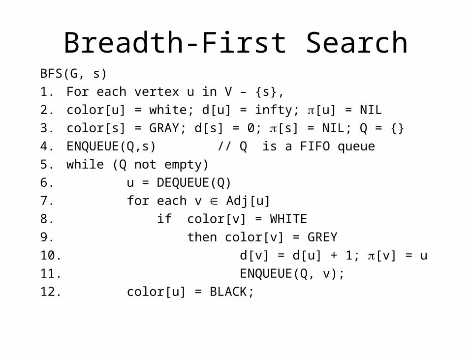
Breadth-First SearchBFS(G, s)

1. For each vertex u in V – {s},

2. color[u] = white; d[u] = infty; [u] = NIL

3. color[s] = GRAY; d[s] = 0; [s] = NIL; Q = {}

4. ENQUEUE(Q,s) // Q is a FIFO queue

5. while (Q not empty)

6. u = DEQUEUE(Q)

7. for each v Adj[u]

8. if color[v] = WHITE

9. then color[v] = GREY

10. d[v] = d[u] + 1; [v] = u

11. ENQUEUE(Q, v);

12. color[u] = BLACK;

Breadth-first Search

• Visited all vertices reachable from the root

• A spanning tree

• For any vertex at level i, the spanning tree path from s to i has i edges, and any other path from s to i has at least i edges (shortest path property)

Breadth-First Search: the Color Scheme

• White vertices have not been discovered– All vertices start out white

• Grey vertices are discovered but not fully explored– They may be adjacent to white vertices

• Black vertices are discovered and fully explored– They are adjacent only to black and gray vertices

• Explore vertices by scanning adjacency list of grey vertices

Graphs with Non-Negative Weights

• Shortest Path Tree

• Can we use a similar idea to generate a shortest path tree which represents the shortest path from s to all vertices that are reachable from s?

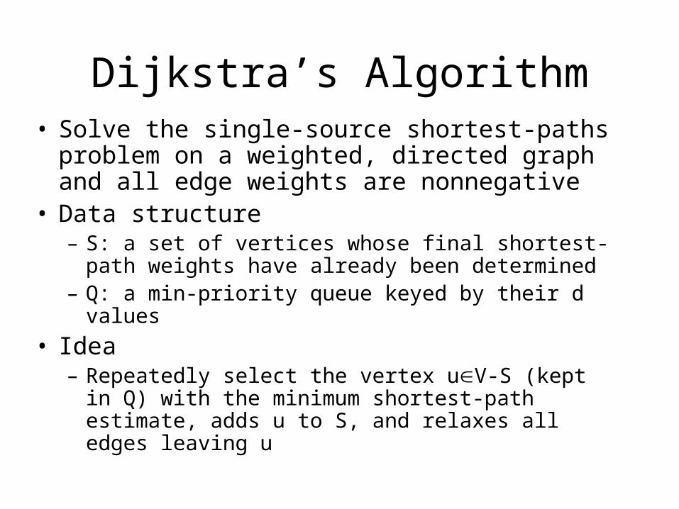
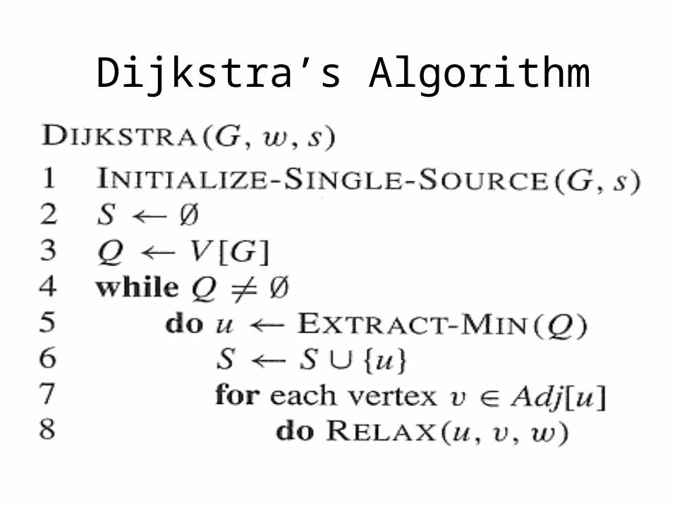
Dijkstra’s Algorithm• Solve the single-source shortest-paths problem on a

weighted, directed graph and all edge weights are nonnegative

• Data structure– S: a set of vertices whose final shortest-path weights have

already been determined– Q: a min-priority queue keyed by their d values

• Idea– Repeatedly select the vertex uV-S (kept in Q) with the

minimum shortest-path estimate, adds u to S, and relaxes all edges leaving u

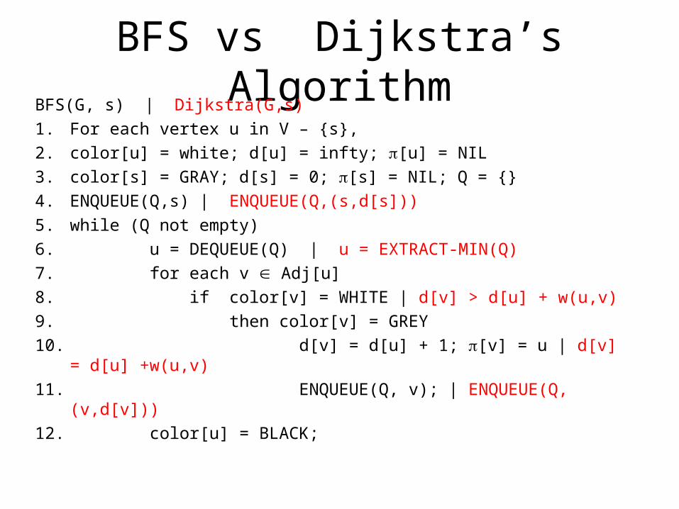
BFS vs Dijkstra’s AlgorithmBFS(G, s) | Dijkstra(G,s)

1. For each vertex u in V – {s},

2. color[u] = white; d[u] = infty; [u] = NIL

3. color[s] = GRAY; d[s] = 0; [s] = NIL; Q = {}

4. ENQUEUE(Q,s) | ENQUEUE(Q,(s,d[s]))

5. while (Q not empty)

6. u = DEQUEUE(Q) | u = EXTRACT-MIN(Q)

7. for each v Adj[u]

8. if color[v] = WHITE | d[v] > d[u] + w(u,v)

9. then color[v] = GREY

10. d[v] = d[u] + 1; [v] = u | d[v] = d[u] +w(u,v)

11. ENQUEUE(Q, v); | ENQUEUE(Q, (v,d[v]))

12. color[u] = BLACK;

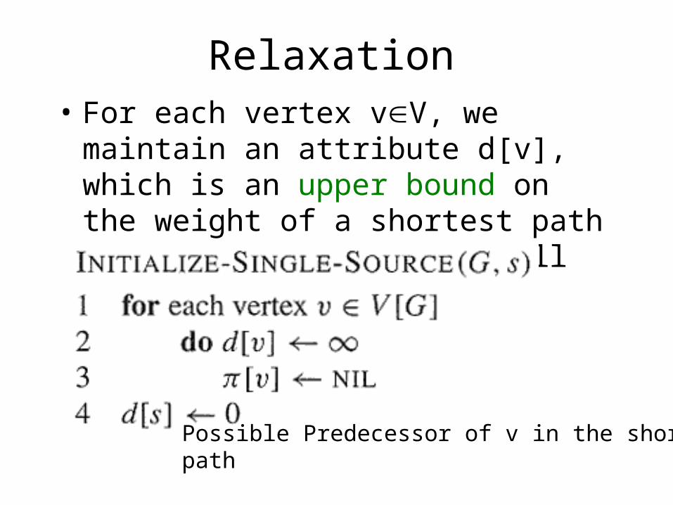
Relaxation• For each vertex vV, we maintain an

attribute d[v], which is an upper bound on the weight of a shortest path from source s to v. We call d[v] a shortest-path estimate.

Possible Predecessor of v in the shortest path

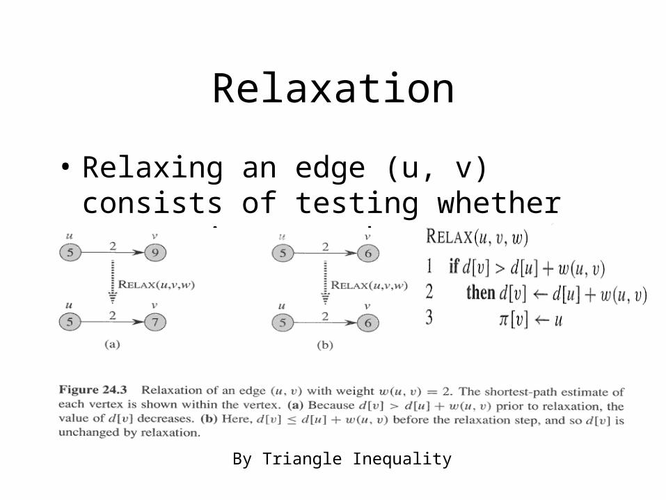
Relaxation

• Relaxing an edge (u, v) consists of testing whether we can improve the shortest path found so far by going through u and, if so, update d[v] and [v]

By Triangle Inequality

Dijkstra’s Algorithm

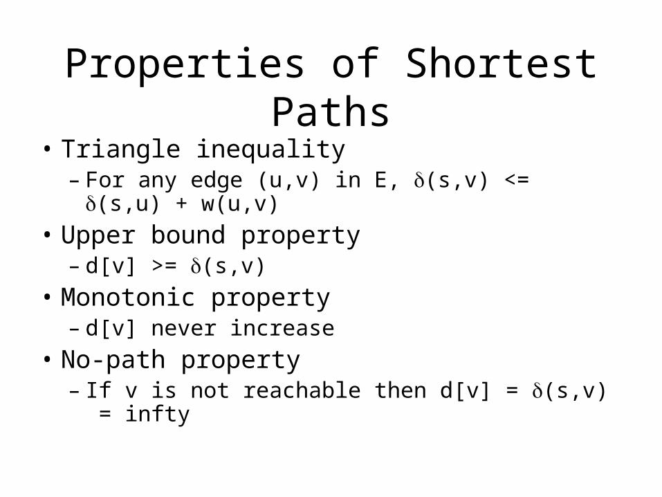
Properties of Shortest Paths

• Triangle inequality– For any edge (u,v) in E, (s,v) <= (s,u) + w(u,v)

• Upper bound property– d[v] >= (s,v)

• Monotonic property – d[v] never increase

• No-path property– If v is not reachable then d[v] = (s,v) = infty

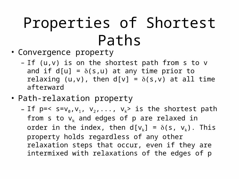
Properties of Shortest Paths• Convergence property

– If (u,v) is on the shortest path from s to v and if d[u] = (s,u) at any time prior to relaxing (u,v), then d[v] = (s,v) at all time afterward

• Path-relaxation property– If p=< s=v0,v1, v2,..., vk> is the shortest path from s to vk

and edges of p are relaxed in order in the index, then d[vk] = (s, vk). This property holds regardless of any other relaxation steps that occur, even if they are intermixed with relaxations of the edges of p

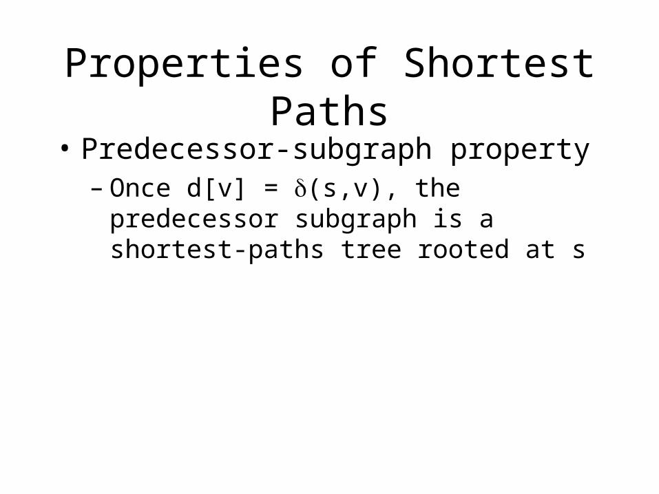
Properties of Shortest Paths

• Predecessor-subgraph property– Once d[v] = (s,v), the predecessor subgraph is

a shortest-paths tree rooted at s

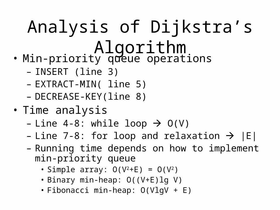
Analysis of Dijkstra’s Algorithm• Min-priority queue operations

– INSERT (line 3)– EXTRACT-MIN( line 5)– DECREASE-KEY(line 8)

• Time analysis– Line 4-8: while loop O(V)– Line 7-8: for loop and relaxation |E| – Running time depends on how to implement min-priority

queue• Simple array: O(V2+E) = O(V2)• Binary min-heap: O((V+E)lg V)• Fibonacci min-heap: O(VlgV + E)