Embed Size (px)
Citation preview
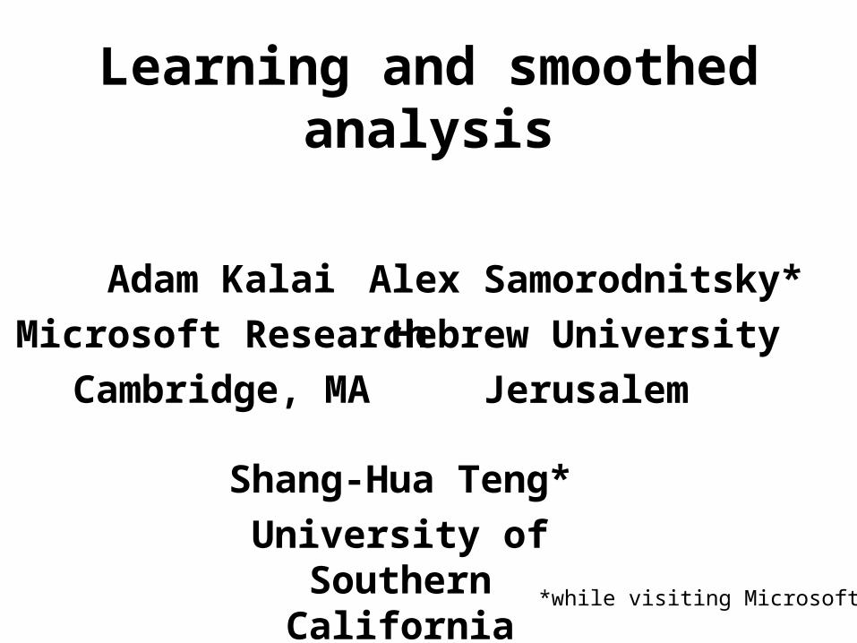
Learning and smoothed analysis
Adam KalaiMicrosoft Research
Cambridge, MA
Shang-Hua Teng*University of Southern
California
Alex Samorodnitsky*Hebrew University
Jerusalem
*while visiting Microsoft
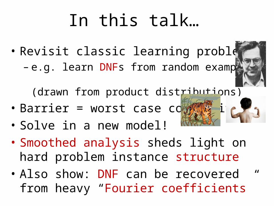
In this talk…
• Revisit classic learning problems– e.g. learn DNFs from random examples
(drawn from product distributions)
• Barrier = worst case complexity• Solve in a new model!• Smoothed analysis sheds light on hard problem
instance structure• Also show: DNF can be recovered from heavy
“Fourier coefficients”
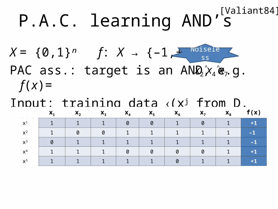
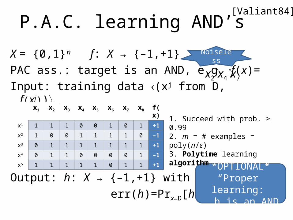
P.A.C. learning AND’s!?
X = {0,1}ⁿ f: X → {–1,+1}PAC ass.: target is an AND, e.g. f(x)=Input: training data (xj from D, f(xj))j≤m
Noiseless
x2˄x4˄x7
x1 x2 x3 x4 x5 x6 x7 x8 f(x)
x1 1 1 1 0 0 1 0 1 +1
x2 1 0 0 1 1 1 1 1 –1
x3 0 1 1 1 1 1 1 1 –1
x4 1 1 1 0 0 0 0 1 +1
x5 1 1 1 1 1 0 1 1 +1
[Valiant84]
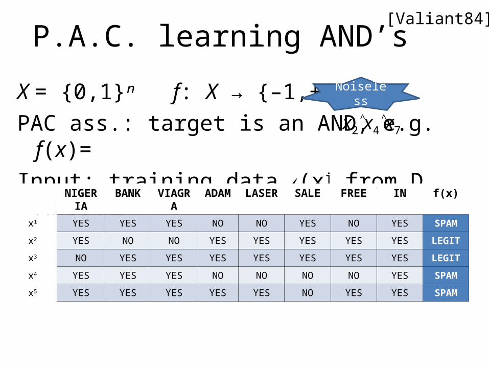
P.A.C. learning AND’s!?
X = {0,1}ⁿ f: X → {–1,+1}PAC ass.: target is an AND, e.g. f(x)=Input: training data (xj from D, f(xj))j≤m
Noiseless
x2˄x4˄x7
NIGERIA BANK VIAGRA ADAM LASER SALE FREE IN f(x)
x1 YES YES YES NO NO YES NO YES SPAM
x2 YES NO NO YES YES YES YES YES LEGIT
x3 NO YES YES YES YES YES YES YES LEGIT
x4 YES YES YES NO NO NO NO YES SPAM
x5 YES YES YES YES YES NO YES YES SPAM
[Valiant84]
P.A.C. learning AND’s!?
X = {0,1}ⁿ f: X → {–1,+1}PAC ass.: target is an AND, e.g. f(x)=Input: training data (xj from D, f(xj))j≤m
Output: h: X → {–1,+1} with err(h)=Prx←D[h(x)≠f(x)] ≤ ε
Noiseless
x2˄x4˄x7
x1 x2 x3 x4 x5 x6 x7 x8 f(x)
x1 1 1 1 0 0 1 0 1 +1
x2 1 0 0 1 1 1 1 0 –1
x3 0 1 1 1 1 1 1 1 +1
x4 0 1 1 0 0 0 0 1 –1
x5 1 1 1 1 1 0 1 1 +1
*OPTIONAL*“Proper” learning:
h is an AND
1. Succeed with prob. ≥ 0.992. m = # examples = poly(n/ε)3. Polytime learning algorithm
[Valiant84]
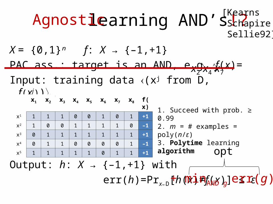
P.A.C. learning AND’s!?Agnostic [Kearns Schapire Sellie92]
X = {0,1}ⁿ f: X → {–1,+1}PAC ass.: target is an AND, e.g. f(x)=Input: training data (xj from D, f(xj))j≤m
Output: h: X → {–1,+1} with err(h)=Prx←D[h(x)≠f(x)] ≤ ε
x1 x2 x3 x4 x5 x6 x7 x8 f(x)
x1 1 1 1 0 0 1 0 1 +1
x2 1 0 0 1 1 1 1 0 –1
x3 0 1 1 1 1 1 1 1 +1
x4 0 1 1 0 0 0 0 1 –1
x5 1 1 1 1 1 0 1 1 +1
1. Succeed with prob. ≥ 0.992. m = # examples = poly(n/ε)3. Polytime learning algorithm
x2˄x4˄x7
opt
+ minAND g err(g)
PAC Agnostic
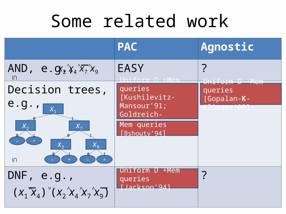
AND, e.g., EASY ?
Decision trees, e.g., ? ?
DNF, e.g., ? ?(x1˄x4)˅(x2˄x4˄x7˄x9)
x2˄x4˄x7˄x9
x1
x2 x7
x9x2+–
+– +–
10
0 1 0 1
0 1 0 1
Uniform D +Mem queries[Kushilevitz-Mansour’91;Goldreich-Levin’89]
Uniform D +Mem queries[Jackson’94]
Uniform D +Mem queries[Gopalan-K-Klivans’08]
Mem queries [Bshouty’94]
Some related work
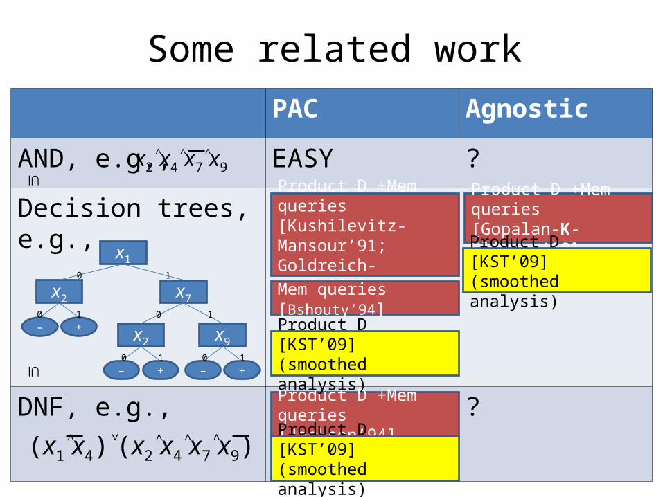
Some related workPAC Agnostic
AND, e.g., EASY ?
Decision trees, e.g., ? ?
DNF, e.g., ? ?(x1˄x4)˅(x2˄x4˄x7˄x9)
x2˄x4˄x7˄x9
x1
x2 x7
x9x2+–
+– +–
10
0 1 0 1
0 1 0 1
Product D +Mem queries[Kushilevitz-Mansour’91;Goldreich-Levin’89]
Product D +Mem queries[Jackson’94]
Product D +Mem queries[Gopalan-K-Klivans’08]
Product D [KST’09] (smoothed analysis)
Product D [KST’09] (smoothed analysis)
Mem queries [Bshouty’94]
Product D [KST’09] (smoothed analysis)

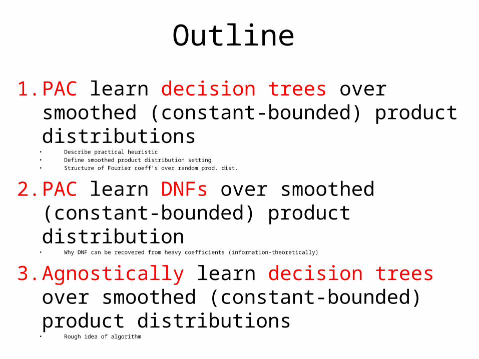
Outline
1. PAC learn decision trees over smoothed (constant-bounded) product distributions
• Describe practical heuristic• Define smoothed product distribution setting• Structure of Fourier coeff’s over random prod. dist.
2. PAC learn DNFs over smoothed (constant-bounded) product distribution
• Why DNF can be recovered from heavy coefficients (information-theoretically)
3. Agnostically learn decision trees over smoothed (constant-bounded) product distributions
• Rough idea of algorithm
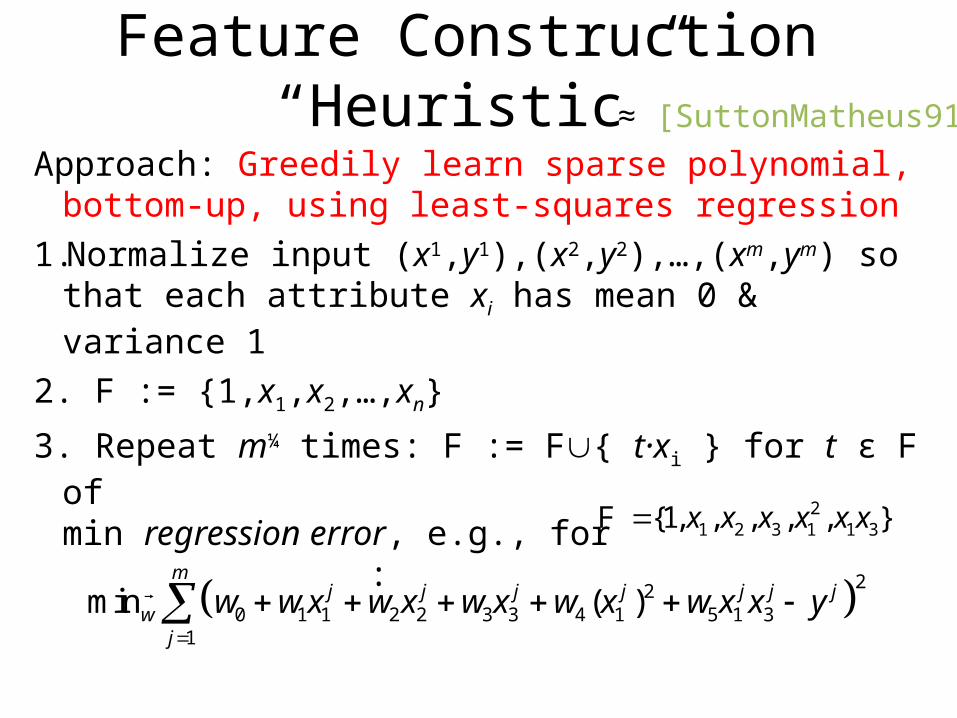
Feature Construction “Heuristic”
Approach: Greedily learn sparse polynomial, bottom-up, using least-squares regression
1.Normalize input (x1,y1),(x2,y2),…,(xm,ym) so that each attribute xi has mean 0 & variance 1
2. F := {1,x1,x2,…,xn}
3. Repeat m¼ times: F := F{ t·xi } for t ϵ F of min regression error, e.g., for :
≈ [SuttonMatheus91]
21 2 3 1 1 3,1, ,{ , , }x x x xx xF
220 1 2 2 3 3 4 1 5 1 31
1
min ( )j jm
j j j
j
jjw w x w x w x w x xw w x y
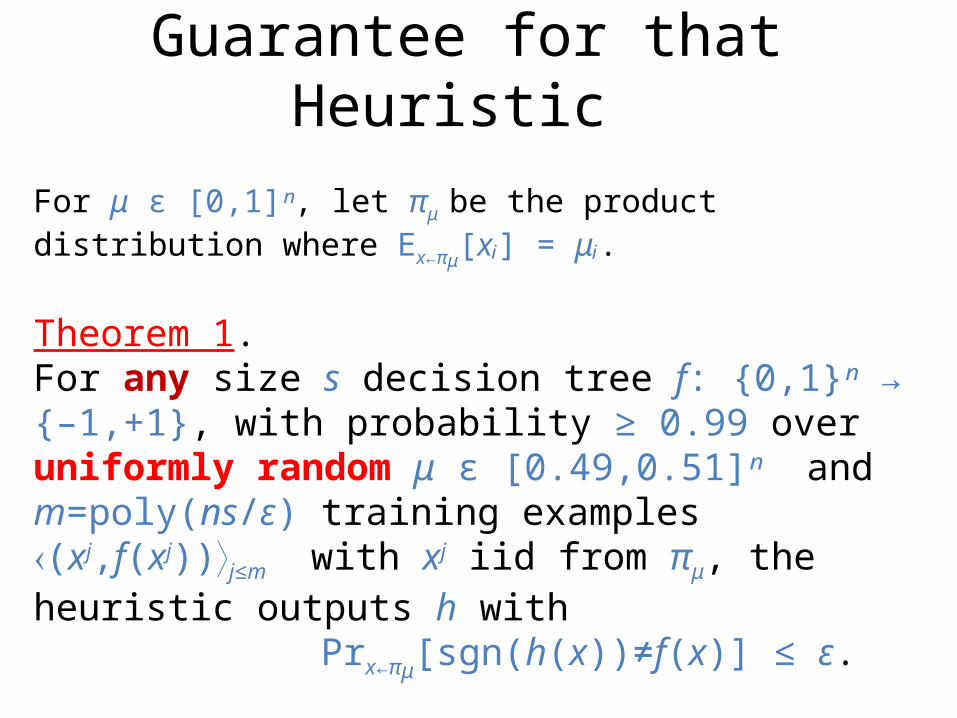
Guarantee for that Heuristic
For μ ϵ [0,1]ⁿ, let πμ be the product distribution where Ex←πμ[xᵢ] = μᵢ.
Theorem 1. For any size s decision tree f: {0,1}ⁿ → {–1,+1}, with probability ≥ 0.99 over uniformly random μ ϵ [0.49,0.51]ⁿ and m=poly(ns/ε) training examples (xj,f(xj))j≤m with xj iid from πμ, the heuristic outputs h with
Prx←πμ[sgn(h(x))≠f(x)] ≤ ε.
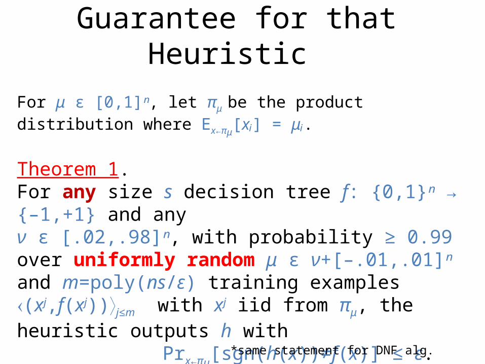
Guarantee for that Heuristic
For μ ϵ [0,1]ⁿ, let πμ be the product distribution where Ex←πμ[xᵢ] = μᵢ.
Theorem 1. For any size s decision tree f: {0,1}ⁿ → {–1,+1} and any ν ϵ [.02,.98]ⁿ, with probability ≥ 0.99 over uniformly random μ ϵ ν+[–.01,.01]ⁿ and m=poly(ns/ε) training examples (xj,f(xj))j≤m with xj iid from πμ, the heuristic outputs h with
Prx←πμ[sgn(h(x))≠f(x)] ≤ ε.
*same statement for DNF alg.
x1
x2 x7
x9x2
–1 –1+1+1
–1 +1
cube ν+[-.01,.01]ⁿ f:{0,1}n{-1,1}
prod dist πμ
(x(1), f(x(1))),…,(x(m),f(x(m))) LEARNINGALG.
iid…
Pr[ h(x) f(x) ] ≤
h
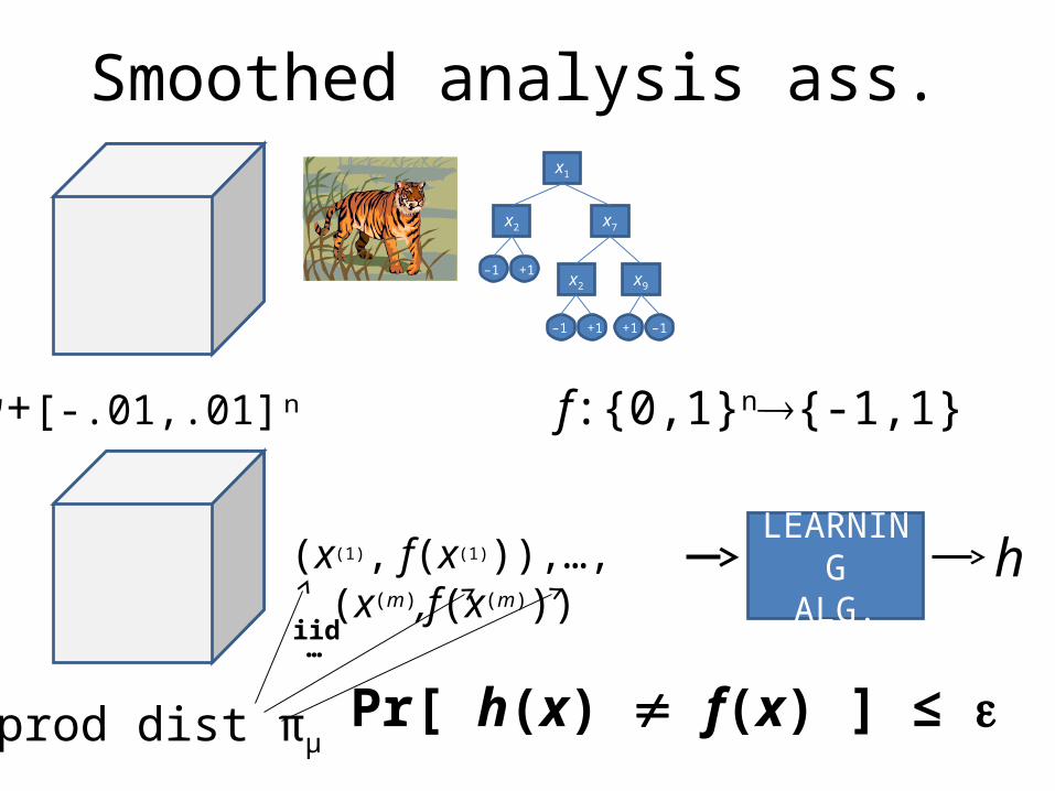
Smoothed analysis ass.
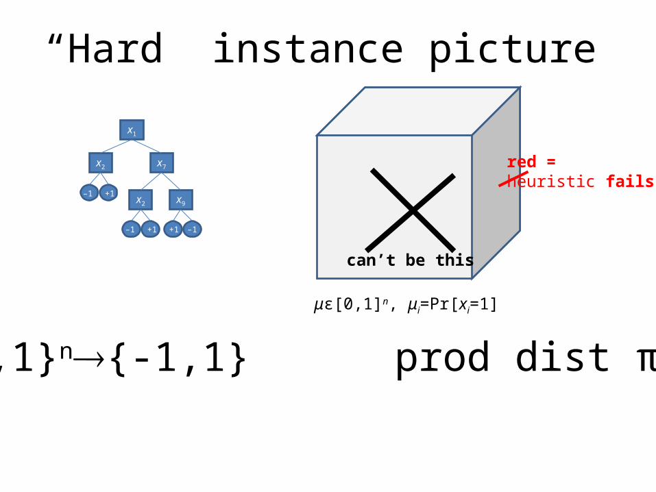
“Hard” instance picture
μϵ[0,1]n, μi=Pr[xi=1]
x1
x2 x7
x9x2
–1 –1+1+1
–1 +1
red =heuristic fails
f:{0,1}n{-1,1} prod dist πμ
can’t be this
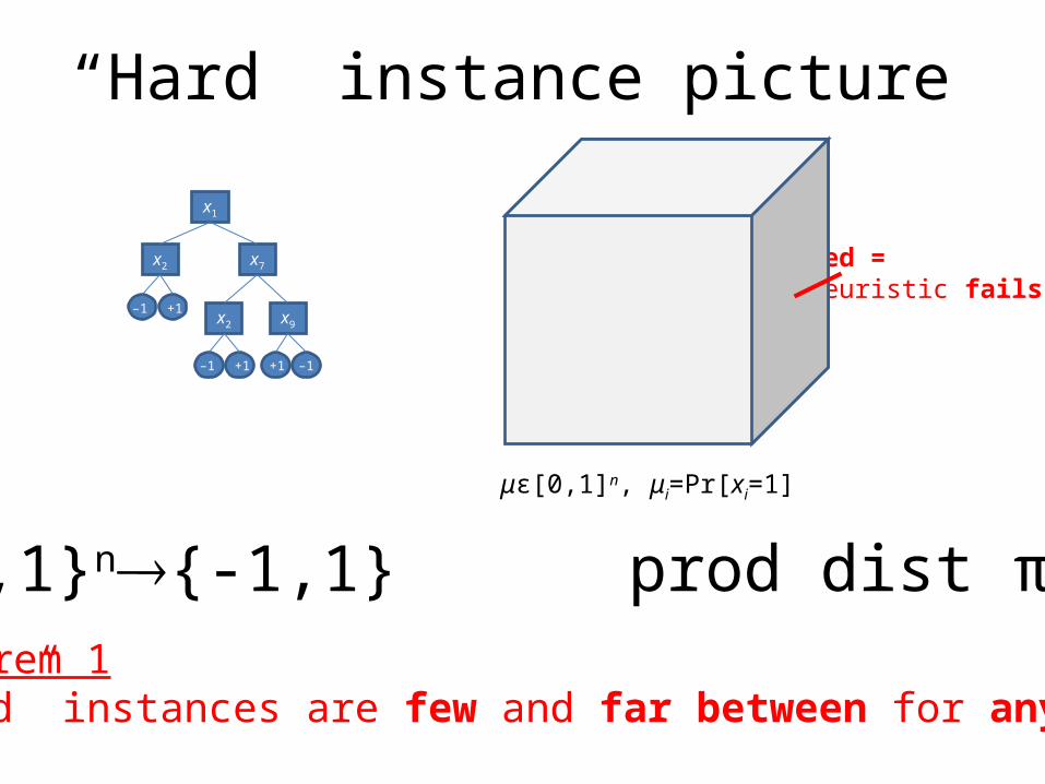
“Hard” instance picture
μϵ[0,1]n, μi=Pr[xi=1]
x1
x2 x7
x9x2
–1 –1+1+1
–1 +1
red =heuristic fails
f:{0,1}n{-1,1} prod dist πμ
Theorem 1“Hard” instances are few and far between for any tree
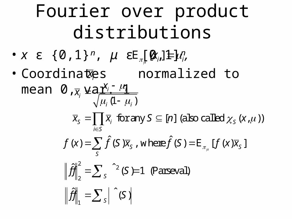
Fourier over product distributions
• x ϵ {0,1}ⁿ, μ ϵ [0,1]ⁿ,
• Coordinates normalized to mean 0, var. 1
1
22
2
(1 )
[ ] (also called ( , ))
ˆ ˆ( ) ( ) ( ) E [ ( ) ]
ˆ ˆ ( ) (Pars
for any
, where
1 eval)
ˆ ˆ ( )
i ii
i i
S i Si S
S SS
S
S
x
n x
f x f S f
x
x x S
x S f x
f f
x
S
f f S
ix
E [ ]i ix
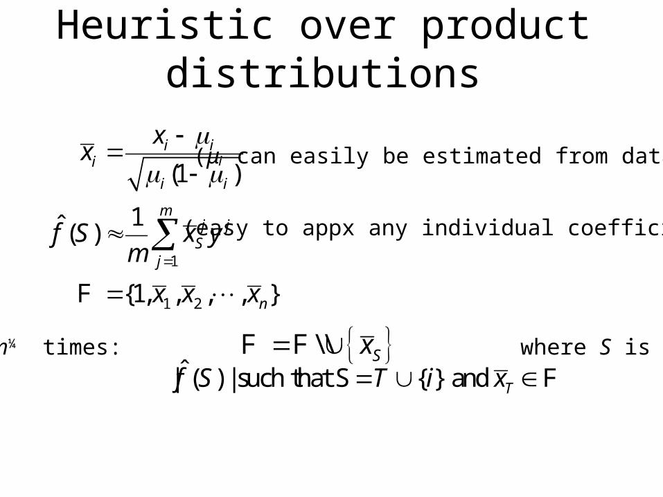
Heuristic over product distributions
1
1 2
(1 )
1ˆ ( )
{1, , , },
i ii
i i
mj j
Sj
n
xx
x
m
x
x y
x
f S
F
(μᵢ can easily be estimated from data)
(easy to appx any individual coefficient)
1)
2)Repeat m¼ times: where S is chosen to
maximize Sx F F \ \
ˆ| ( ) | such that S { } and Txf S T i F
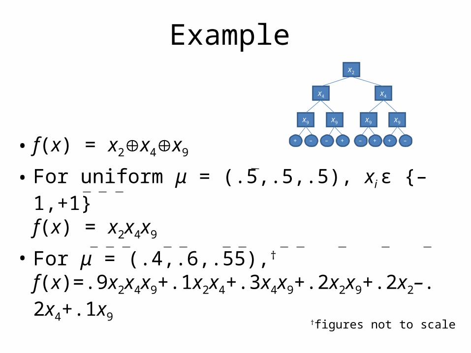
Example
• f(x) = x2x4x9
• For uniform μ = (.5,.5,.5), xi ϵ {–1,+1}f(x) = x2x4x9
• For μ = (.4,.6,.55),† f(x)=.9x2x4x9+.1x2x4+.3x4x9+.2x2x9+.2x2–.2x4+.1x9
x2
x4 x4
x9x9
+
x9x9
+ –––– +++
†figures not to scale
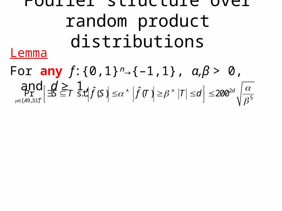
Fourier structure over random product distributions
LemmaFor any f:{0,1}ⁿ→{–1,1}, α,β > 0, and d ≥ 1,
25[.49,.51]
ˆ ˆPr s.t. ( ) ( ) 200n
dS T f S f T T d
Fourier structure over random product distributions
LemmaFor any f:{0,1}ⁿ→{–1,1}, α,β > 0, and d ≥ 1,
LemmaLet p:Rⁿ→R be a degree-d multilinear polynomial
with leading coefficient of 1. Then, for any ε>0,
25[.49,.51]
ˆ ˆPr s.t. ( ) ( ) 200n
dS T f S f T T d
[ 1,1]Pr ( ) 2
n
d
xp x
ò ò e.g., p(x)=x1x2x9+.3x7–0.2
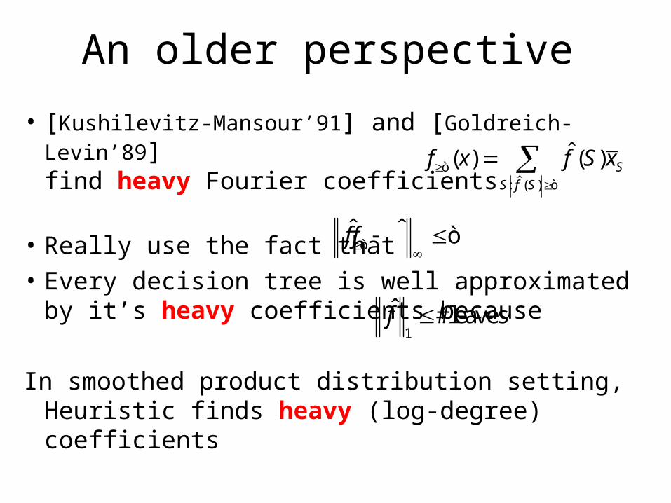
An older perspective
• [Kushilevitz-Mansour’91] and [Goldreich-Levin’89]find heavy Fourier coefficients
• Really use the fact that • Every decision tree is well approximated by it’s
heavy coefficients because
In smoothed product distribution setting, Heuristic finds heavy (log-degree) coefficients
ˆ ( ):
ˆ (( ) ) SfS S
f S xf x
òò
ˆ ˆf f
ò ò
1
ˆ #leavesf
Outline
1. PAC learn decision trees over smoothed (constant-bounded) product distributions
• Describe practical heuristic• Define smoothed product distribution setting• Structure of Fourier coeff’s over random prod. dist.
2. PAC learn DNFs over smoothed (constant-bounded) product distribution
• Why DNF can be recovered from heavy coefficients (information-theoretically)
3. Agnostically learn decision trees over smoothed (constant-bounded) product distributions
• Rough idea of algorithm
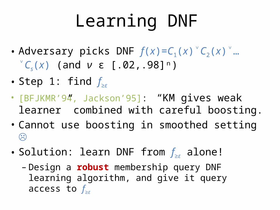
Learning DNF
• Adversary picks DNF f(x)=C1(x)˅C2(x)˅…˅Cs(x) (and ν ϵ [.02,.98]ⁿ)
• Step 1: find f≥ε
• [BFJKMR’94, Jackson’95]: “KM gives weak learner” combined with careful boosting.
• Cannot use boosting in smoothed setting • Solution: learn DNF from f≥ε alone!
– Design a robust membership query DNF learning algorithm, and give it query access to f≥ε
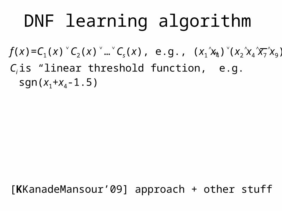
DNF learning algorithm
f(x)=C1(x)˅C2(x)˅…˅Cs(x), e.g., (x1˄x4)˅(x2˄x4˄x7˄x9)
Ci is “linear threshold function,” e.g. sgn(x1+x4-1.5)
[KKanadeMansour’09] approach + other stuff
I’m a burier (of details)
burier noun, pl. –s, One that buries.
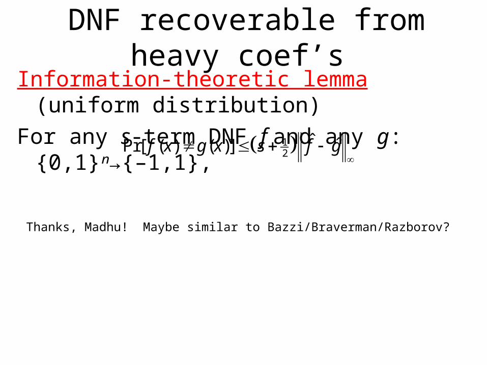
DNF recoverable from heavy coef’sInformation-theoretic lemma (uniform distribution)For any s-term DNF f and any g: {0,1}ⁿ→{–1,1},
12
ˆ ˆPr[ ( ) ( )]f x g x s f g
Thanks, Madhu! Maybe similar to Bazzi/Braverman/Razborov?
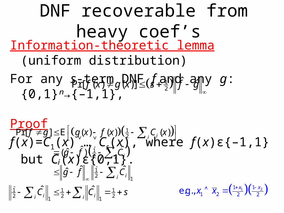
DNF recoverable from heavy coef’sInformation-theoretic lemma (uniform distribution)For any s-term DNF f and any g: {0,1}ⁿ→{–1,1},
Prooff(x)=C1(x)˅…˅Cs(x), where f(x)ϵ{–1,1} but Cᵢ(x)ϵ{0,1}.
12
ˆ ˆPr[ ( ) ( )]f x g x s f g
12Pr[ ] E ( ) ( ) ( )ii
f g g x f x C x 1̂
2
1̂2
1
1̂ 1 12 2 2
1 1
ˆ ˆˆ( )·
ˆ ˆˆ
ˆ ˆ
ii
ii
i ii i
g f C
g f C
C C s
1 21 11 2 2 2e.g., x xx x

Outline
1. PAC learn decision trees over smoothed (constant-bounded) product distributions
• Describe practical heuristic• Define smoothed product distribution setting• Structure of Fourier coeff’s over random prod. dist.
2. PAC learn DNFs over smoothed (constant-bounded) product distribution
• Why heavy coefficients characterize a DNF
3. Agnostically learn decision trees over smoothed (constant-bounded) product distributions
• Rough idea of algorithm
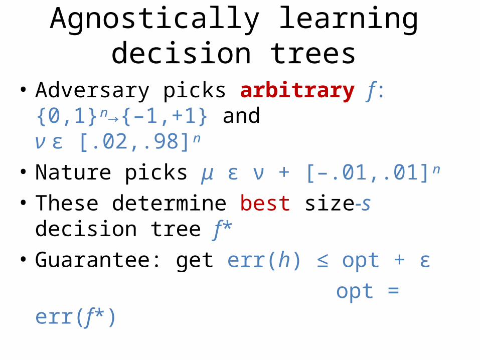
Agnostically learning decision trees
• Adversary picks arbitrary f:{0,1}ⁿ→{–1,+1} andν ϵ [.02,.98]ⁿ
• Nature picks μ ϵ ν + [–.01,.01]ⁿ • These determine best size-s decision tree f*• Guarantee: get err(h) ≤ opt + ε opt = err(f*)
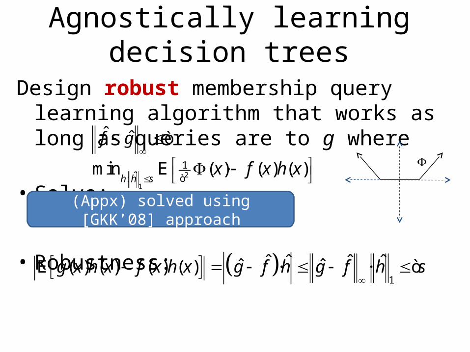
Agnostically learning decision trees
Design robust membership query learning algorithm that works as long as queries are to g where .
• Solve:
• Robustness:
ˆ ˆf g
ò
2
1
1ˆ:
min (E () ) ( )h h s
f x h xx ò
1
ˆ ˆ ˆ ˆˆ ˆ·E ( ) ( ) ( ) ( ·) g f h g f hg x h x f x sh x
ò
(Appx) solved using [GKK’08] approach
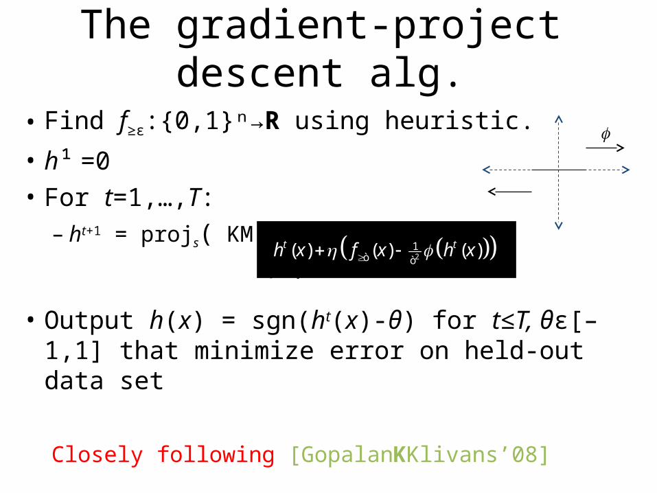
The gradient-project descent alg.
• Find f≥ε:{0,1}ⁿ→R using heuristic.
• h¹ =0
• For t=1,…,T: – ht+1 = projs( KM( ) )
• Output h(x) = sgn(ht(x)-θ) for t≤T, θϵ[–1,1] that minimize error on held-out data set
Closely following [GopalanKKlivans’08]
21( ) ( ) ( )t th x f x h x ò ò
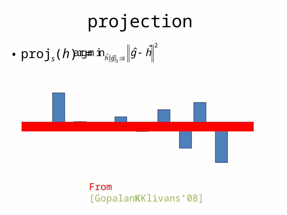
projection
• projs(h) = 1
2
ˆ ˆ:ˆˆarg min
h g sg h
From [GopalanKKlivans’08]
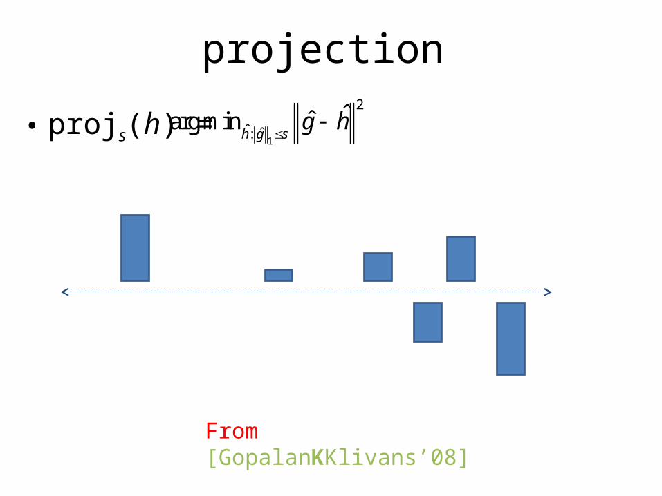
projection
• projs(h) = 1
2
ˆ ˆ:ˆˆarg min
h g sg h
From [GopalanKKlivans’08]
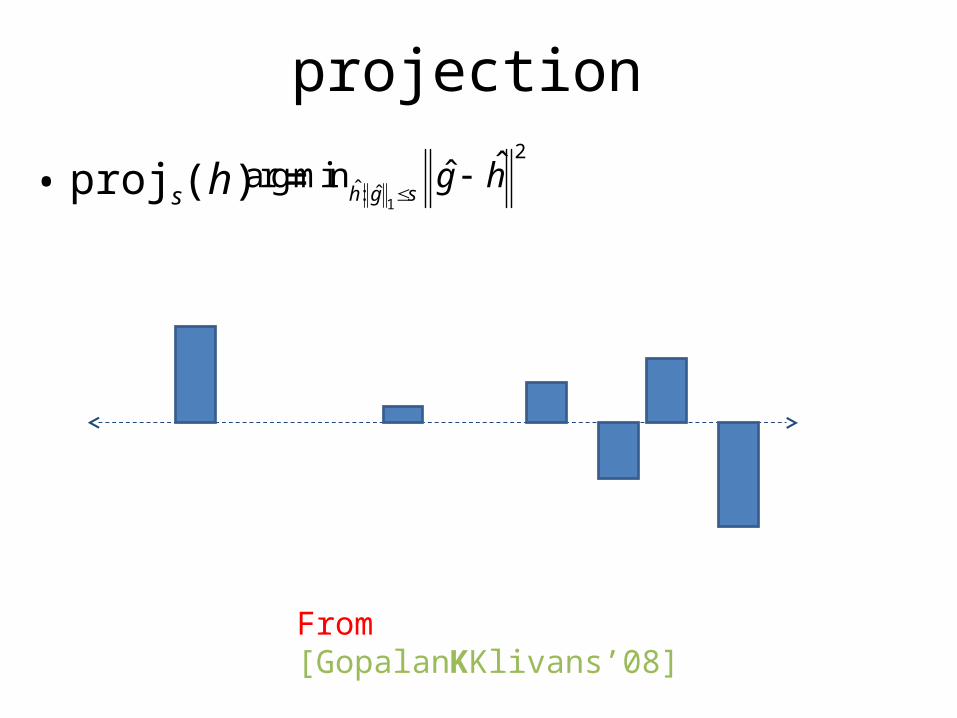
projection
• projs(h) = 1
2
ˆ ˆ:ˆˆarg min
h g sg h
From [GopalanKKlivans’08]
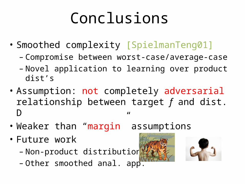
Conclusions
• Smoothed complexity [SpielmanTeng01]– Compromise between worst-case/average-case – Novel application to learning over product dist’s
• Assumption: not completely adversarial relationship between target f and dist. D
• Weaker than “margin” assumptions• Future work
– Non-product distributions– Other smoothed anal. app.

Thanks!Sorry!
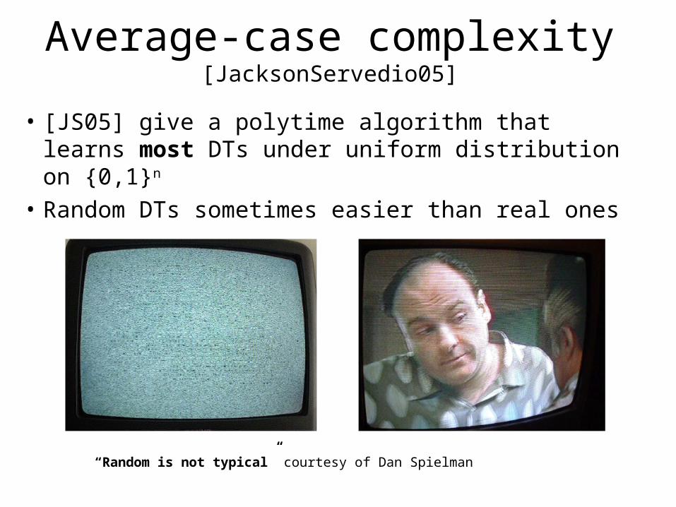
Average-case complexity [JacksonServedio05]
• [JS05] give a polytime algorithm that learns most DTs under uniform distribution on {0,1}n
• Random DTs sometimes easier than real ones
“Random is not typical” courtesy of Dan Spielman

![Smoothed Analysis of the Condition Numbers and Growth Factors … · 2009-11-14 · the algorithm performs poorly. (See also the Smoothed Analysis Homepage [Smo]) Smoothed analysis](https://img.pdfslide.us/doc/110x75/5e9273249dce0d4d044b7179/smoothed-analysis-of-the-condition-numbers-and-growth-factors-2009-11-14-the-algorithm.jpg)


![Engineering DRAWING VAB1012 Lecture 1 by Kalai [Compatibility Mode]](https://img.pdfslide.us/doc/110x75/577d27491a28ab4e1ea3867a/engineering-drawing-vab1012-lecture-1-by-kalai-compatibility-mode.jpg)