Lecture 19 Image processing - cs.brown.edu

Lecture 19Image processing

1

Lecture 19 Outline:

Image Processing (in MATLAB):• Image Processing Toolbox

• imread• imwrite

• Image Data• Vectorizing computations

•Example Transformations• Mirroring• Color to grayscale• Negative• Median noise filter• Edge detection

2

318-by-250

49 55 58 59 57 53 60 67 71 72 72 70 102 108 111 111 112 112 157 167 169 167 165 164 196 205 208 207 205 205 199 208 212 214 213 216 190 192 193 195 195 197 174 169 165 163 162 161

Images are stored as a bunch of numbers

3

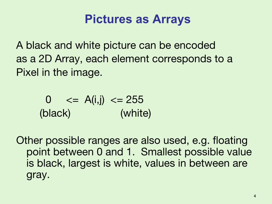
Pictures as Arrays

A black and white picture can be encodedas a 2D Array, each element corresponds to aPixel in the image. 0 <= A(i,j) <= 255 (black) (white)

Other possible ranges are also used, e.g. floating point between 0 and 1. Smallest possible value is black, largest is white, values in between are gray.

4

Pixel Indexing in MATLAB

5

For an image A• A(1,1) is upper left corner pixel of image• A(end,1) is lower left corner pixel • A(1,end) is upper right corner• A(end,end) is lower right corner

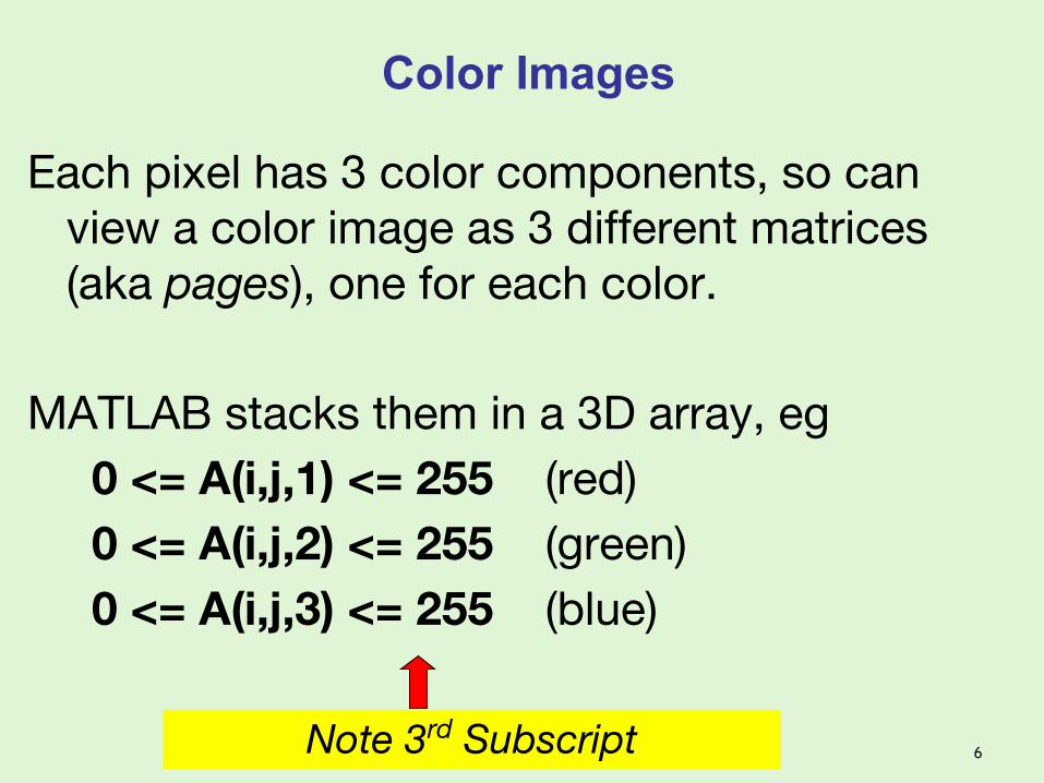
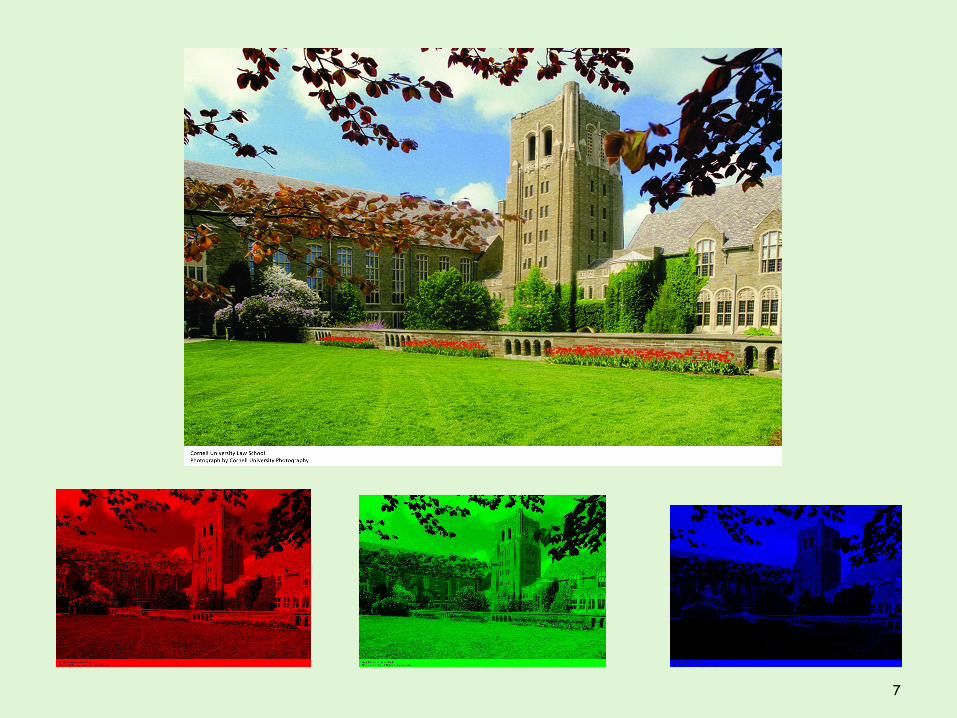
Color Images

Each pixel has 3 color components, so can view a color image as 3 different matrices (aka pages), one for each color.

MATLAB stacks them in a 3D array, eg 0 <= A(i,j,1) <= 255 (red) 0 <= A(i,j,2) <= 255 (green) 0 <= A(i,j,3) <= 255 (blue)

Note 3rd Subscript 6

7

Storing Images

There are a lot of file formats for images. Some common ones:

JPEG (Joint Photographic Experts Group)GIF (Graphics Interchange Format)PNG (Portable Network Graphics)

8

Storing Images

Why are there so many formats?• Different Compression Algorithms

– Lossy (JPEG, GIF)– Lossless (PNG)

• Need for additional attributes– Patient Name, Radiologist Comments, etc. (DICOM)

• Intellectual Property Rights, Royalties

9

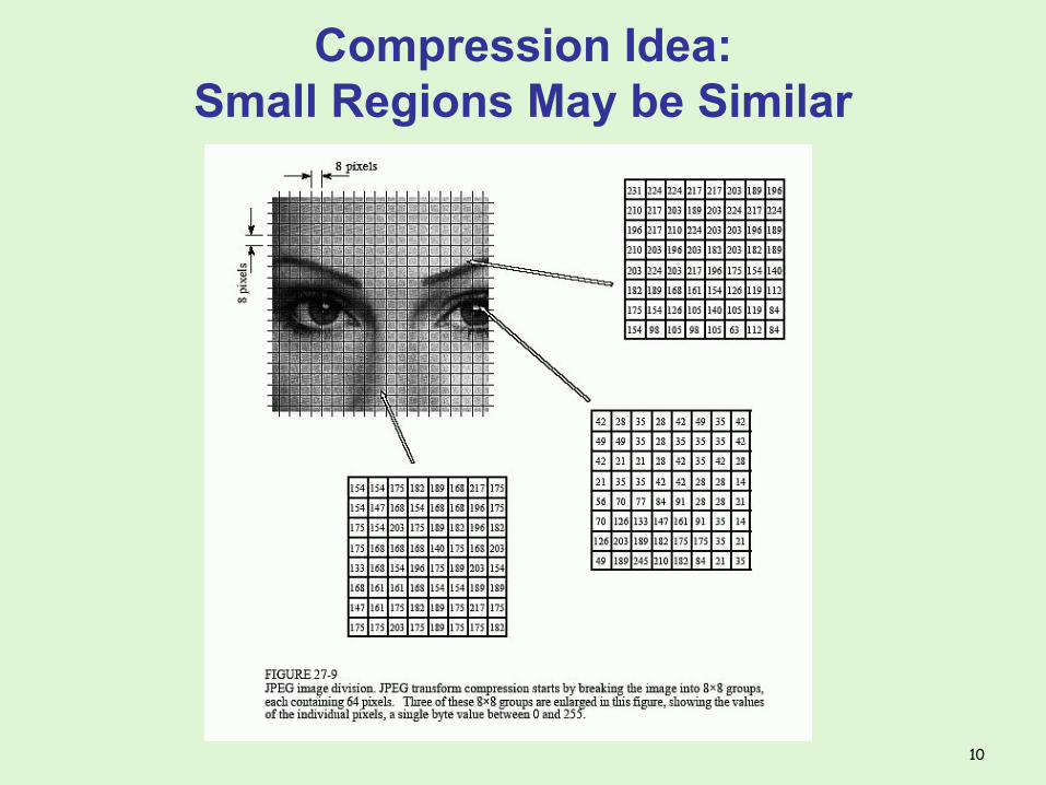
Compression Idea: Small Regions May be Similar

10

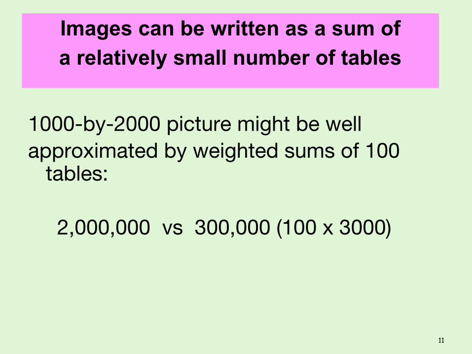
Images can be written as a sum ofa relatively small number of tables

1000-by-2000 picture might be wellapproximated by weighted sums of 100

tables:

2,000,000 vs 300,000 (100 x 3000)

11

Operations on Images

Amount to operations on 2D and 3D Arrays.

A good place to practice “array” thinking.

12

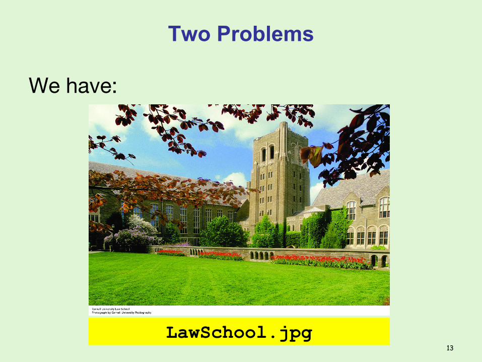
Two Problems

We have:

LawSchool.jpg13

Problem 1

Want:

LawSchoolMirror.jpg

14

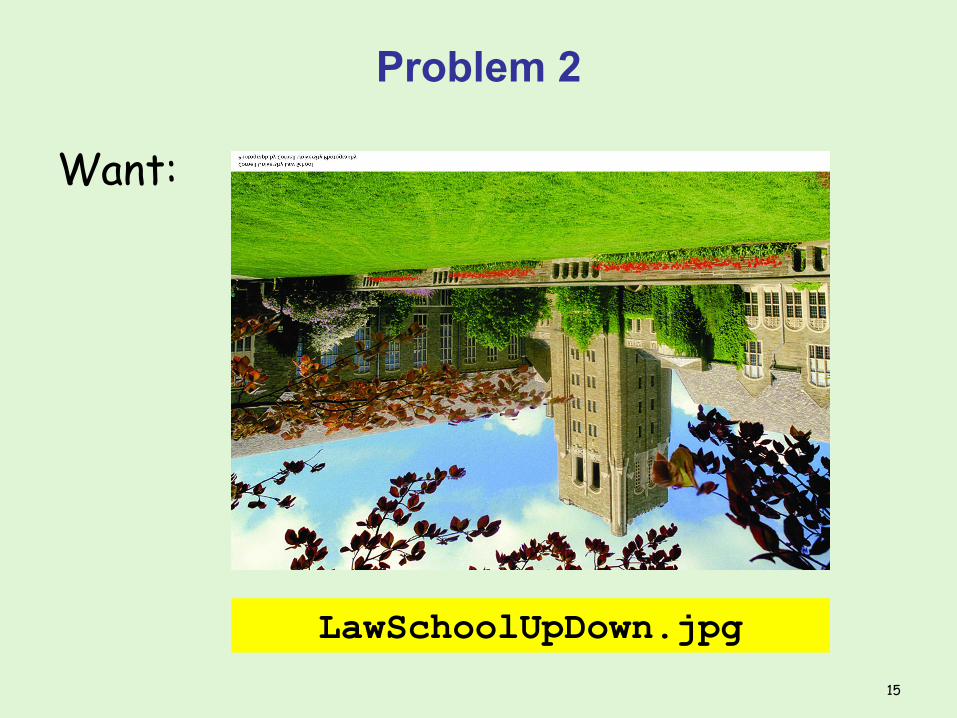
Problem 2

Want:

LawSchoolUpDown.jpg

15

Solution Framework

Read LawSchool.jpg from disk and convert it into an array.

Manipulate the Array.

Convert the array to a jpg file and write it to memory.

16

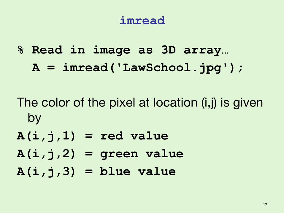
imread

% Read in image as 3D array… A = imread('LawSchool.jpg');

The color of the pixel at location (i,j) is given by

A(i,j,1) = red valueA(i,j,2) = green valueA(i,j,3) = blue value

17

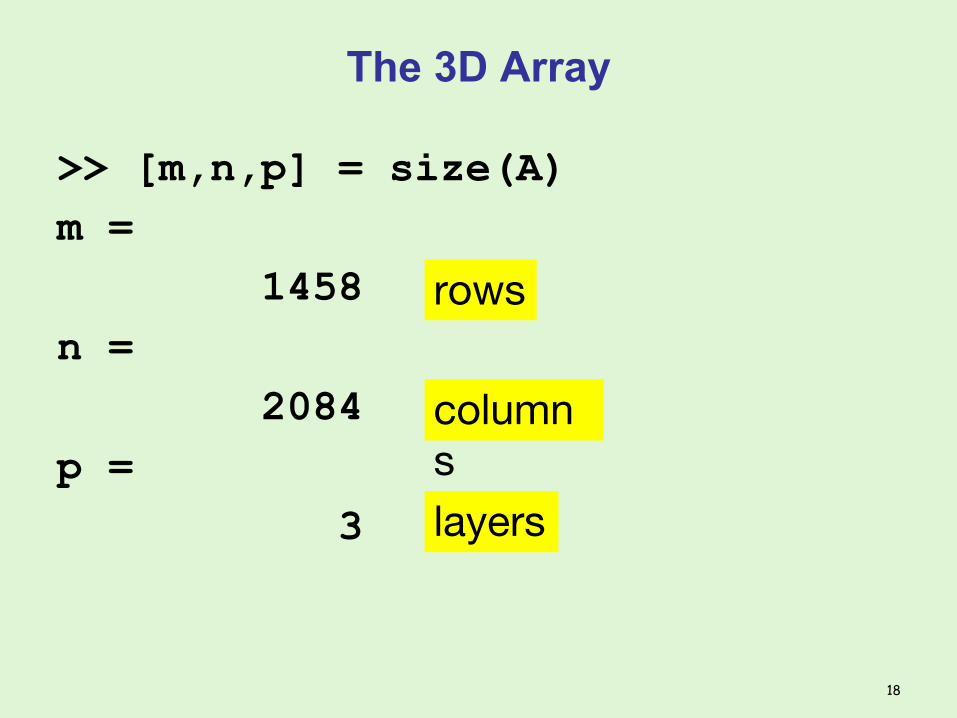
The 3D Array

>> [m,n,p] = size(A)m = 1458n = 2084p = 3

rows

columnslayers

18

The Layers

1458-by-2084

1458-by-2084

1458-by-2084

A(:,:,1)

A(:,:,3)

A(:,:,2)

19

How can we find the Mirror image of A?

20

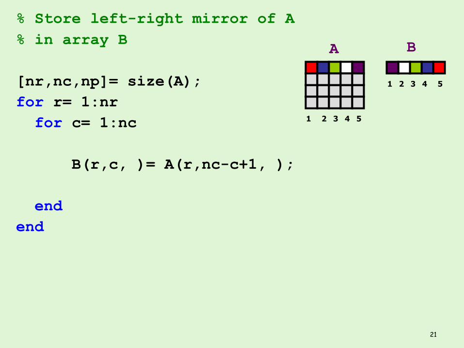
% Store left-right mirror of A% in array B

[nr,nc,np]= size(A);for r= 1:nr for c= 1:nc B(r,c, )= A(r,nc-c+1, ); endend

A B

1

5

2

4

3

3

4

2

5

1

21

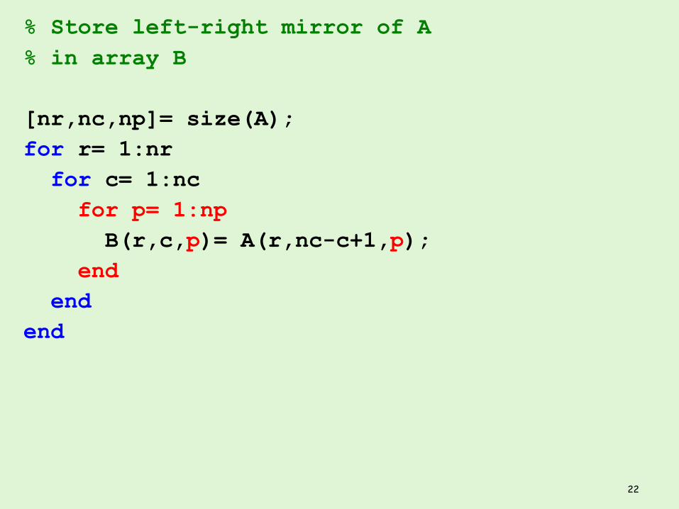
% Store left-right mirror of A% in array B

[nr,nc,np]= size(A);for r= 1:nr for c= 1:nc for p= 1:np B(r,c,p)= A(r,nc-c+1,p); end endend

22

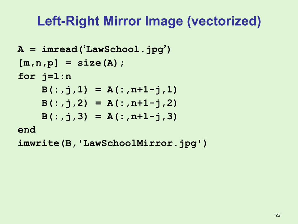
Left-Right Mirror Image (vectorized)

A = imread(’LawSchool.jpg’)[m,n,p] = size(A);for j=1:n B(:,j,1) = A(:,n+1-j,1) B(:,j,2) = A(:,n+1-j,2) B(:,j,3) = A(:,n+1-j,3)endimwrite(B,'LawSchoolMirror.jpg')

23

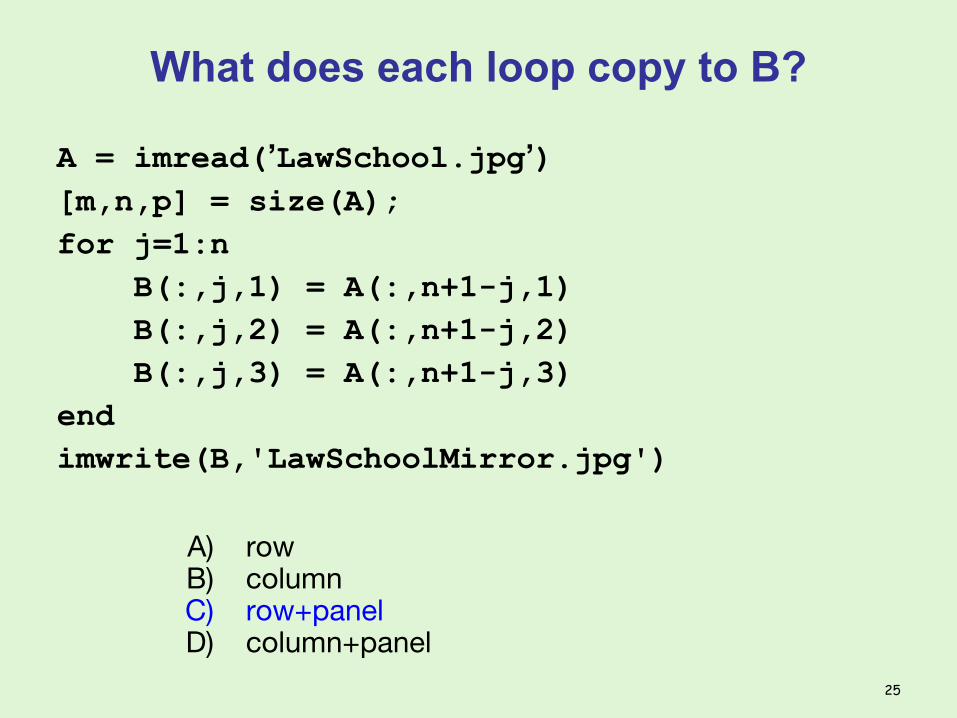
What does each loop copy to B?


24

A) rowB) columnC) row+panelD) column+panel

What does each loop copy to B?


25

A) rowB) columnC) row+panelD) column+panel

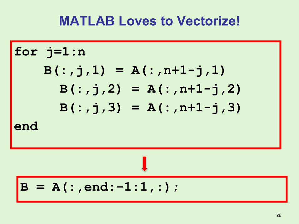
MATLAB Loves to Vectorize!

for j=1:n B(:,j,1) = A(:,n+1-j,1)

B(:,j,2) = A(:,n+1-j,2) B(:,j,3) = A(:,n+1-j,3)

end

B = A(:,end:-1:1,:);

26

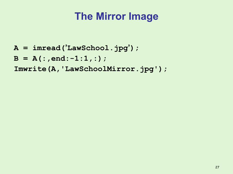
The Mirror Image

A = imread(’LawSchool.jpg’);B = A(:,end:-1:1,:);Imwrite(A,'LawSchoolMirror.jpg');

27

The Upside Down Image

A = imread(’LawSchool.jpg’);C = _______imwrite(C,'LawSchoolUpDown.jpg');

A) C(:,:,end:-1:1)B) C(:,end:-1:1,:)C) C(end:-1:1,:,:)D) I don’t know

28

The Upside Down Image

A = imread(’LawSchool.jpg’);C = _______imwrite(C,'LawSchoolUpDown.jpg');

A) C(:,:,end:-1:1)B) C(:,end:-1:1,:)C) C(end:-1:1,:,:)D) I don’t know

29

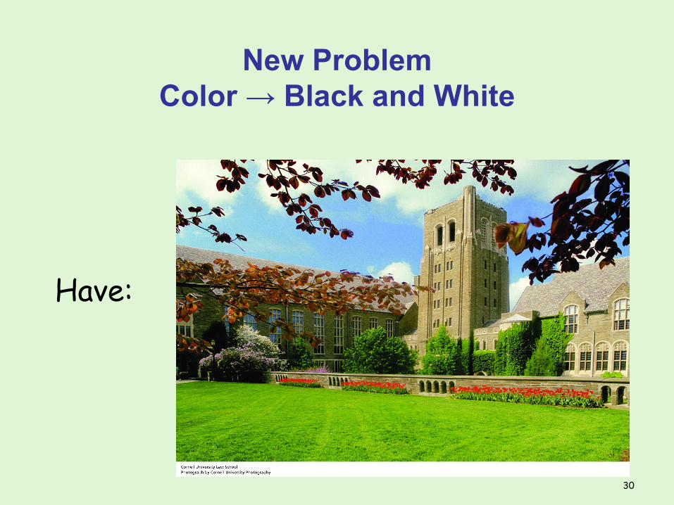
New ProblemColor → Black and White

Have:

30

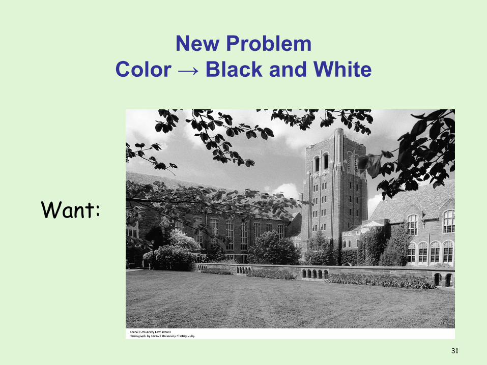
New ProblemColor → Black and White

Want:

31

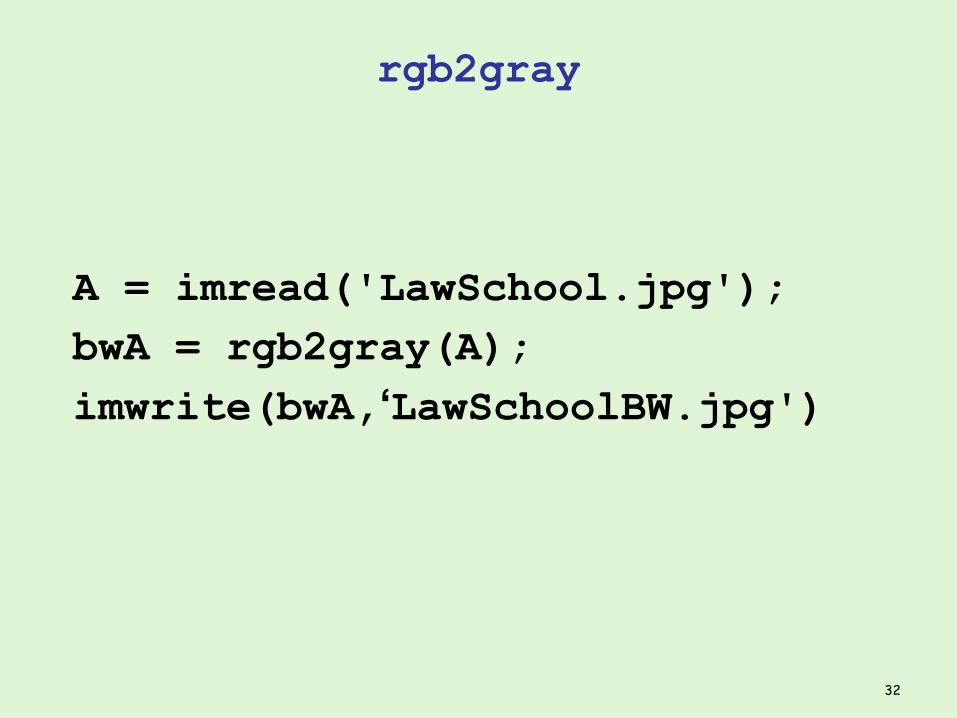
rgb2gray

A = imread('LawSchool.jpg');bwA = rgb2gray(A);imwrite(bwA,‘LawSchoolBW.jpg')

32

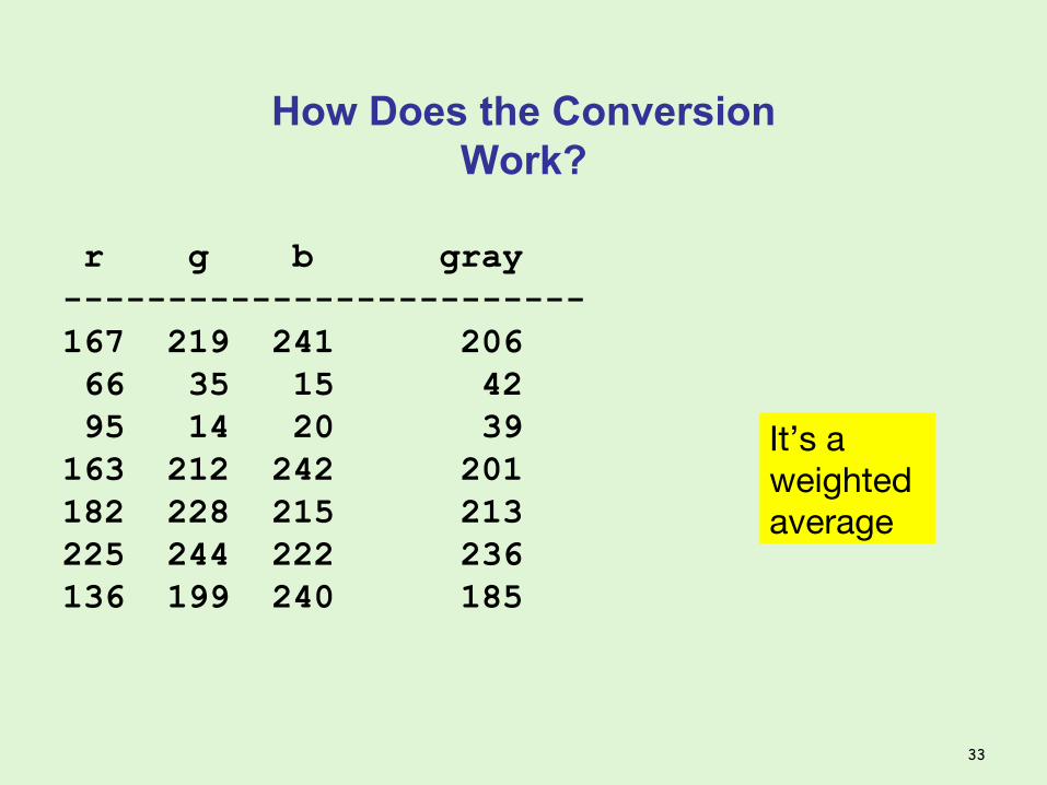
How Does the ConversionWork?

r g b gray-------------------------167 219 241 206 66 35 15 42 95 14 20 39163 212 242 201182 228 215 213225 244 222 236136 199 240 185

It’s a weightedaverage

33

rgb2gray:

34

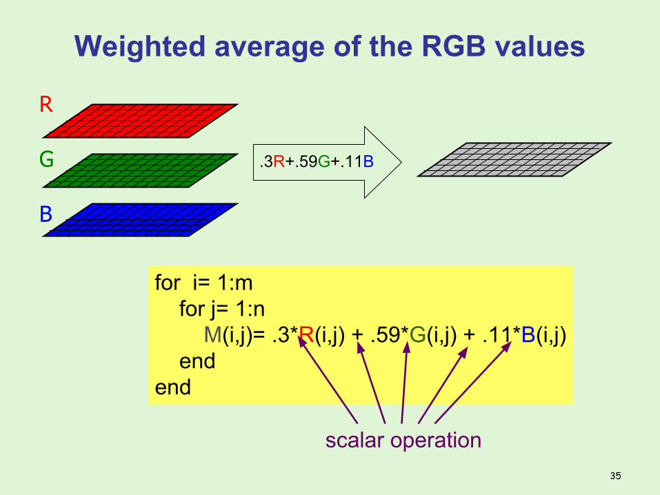
Weighted average of the RGB values

.3R+.59G+.11B

for i= 1:m for j= 1:n M(i,j)= .3*R(i,j) + .59*G(i,j) + .11*B(i,j) endend

scalar operation

R

G

B

35

Why a Weighted Average?

• Due to the way our visual system works• We are most sensitive to Green, then Red

then Blue• Other approaches are close

– Equal Weights (i.e. (r+g+b)/3)– max(r, g, b)

36

Weighted average of the RGB values

.3R+.59G+.11B

M= .3*R + .59*G + .11*B

vectorized operation

R

G

B

37

Coding Average

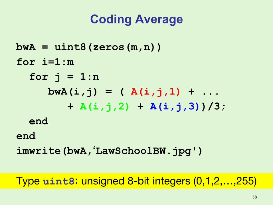
bwA = uint8(zeros(m,n))for i=1:m for j = 1:n bwA(i,j) = ( A(i,j,1) + ... + A(i,j,2) + A(i,j,3))/3; endendimwrite(bwA,‘LawSchoolBW.jpg')

Type uint8: unsigned 8-bit integers (0,1,2,…,255)38

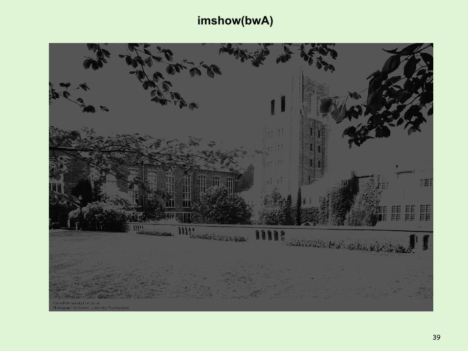
39

imshow(bwA)

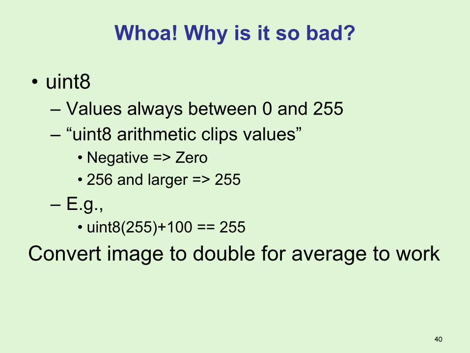
Whoa! Why is it so bad?

• uint8– Values always between 0 and 255– “uint8 arithmetic clips values”

• Negative => Zero• 256 and larger => 255

– E.g., • uint8(255)+100 == 255

Convert image to double for average to work

40

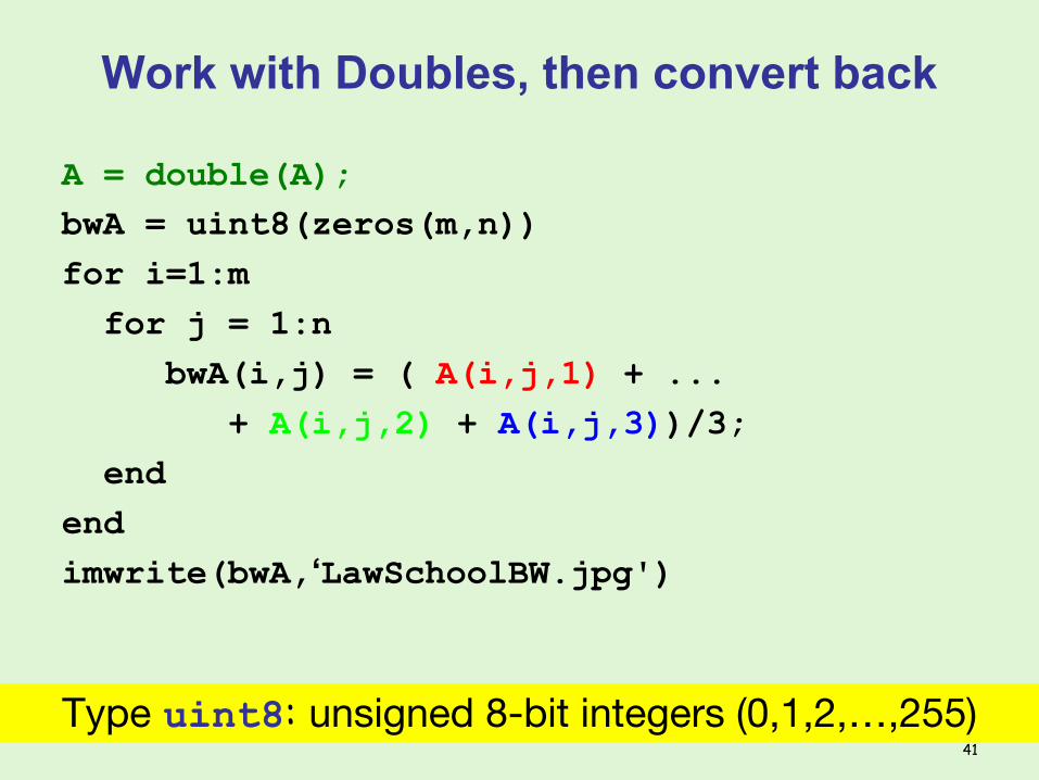
Work with Doubles, then convert back

A = double(A);bwA = uint8(zeros(m,n))for i=1:m for j = 1:n bwA(i,j) = ( A(i,j,1) + ... + A(i,j,2) + A(i,j,3))/3; endendimwrite(bwA,‘LawSchoolBW.jpg')

Type uint8: unsigned 8-bit integers (0,1,2,…,255)41

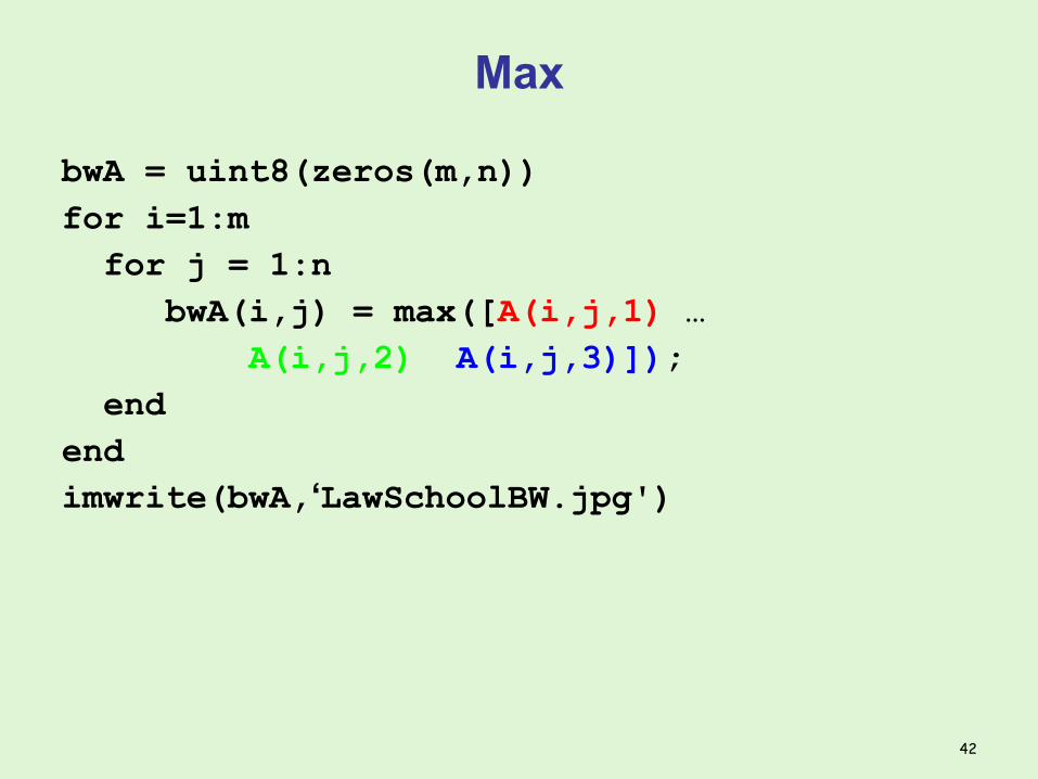
Max

bwA = uint8(zeros(m,n))for i=1:m for j = 1:n bwA(i,j) = max([A(i,j,1) … A(i,j,2) A(i,j,3)]); endendimwrite(bwA,‘LawSchoolBW.jpg')

42

Max:

43

Vectorized Max?

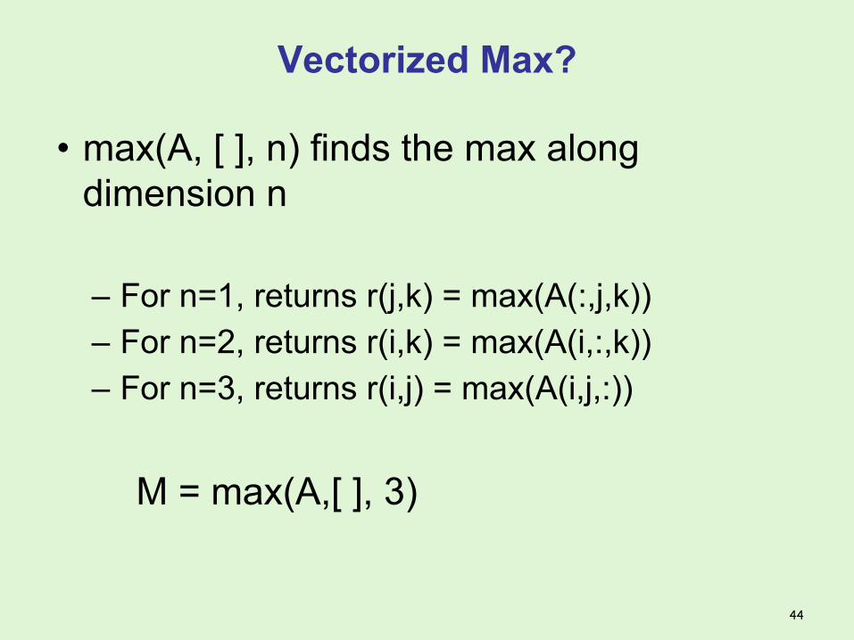
• max(A, [ ], n) finds the max along dimension n

– For n=1, returns r(j,k) = max(A(:,j,k))– For n=2, returns r(i,k) = max(A(i,:,k))– For n=3, returns r(i,j) = max(A(i,j,:))

M = max(A,[ ], 3)

44

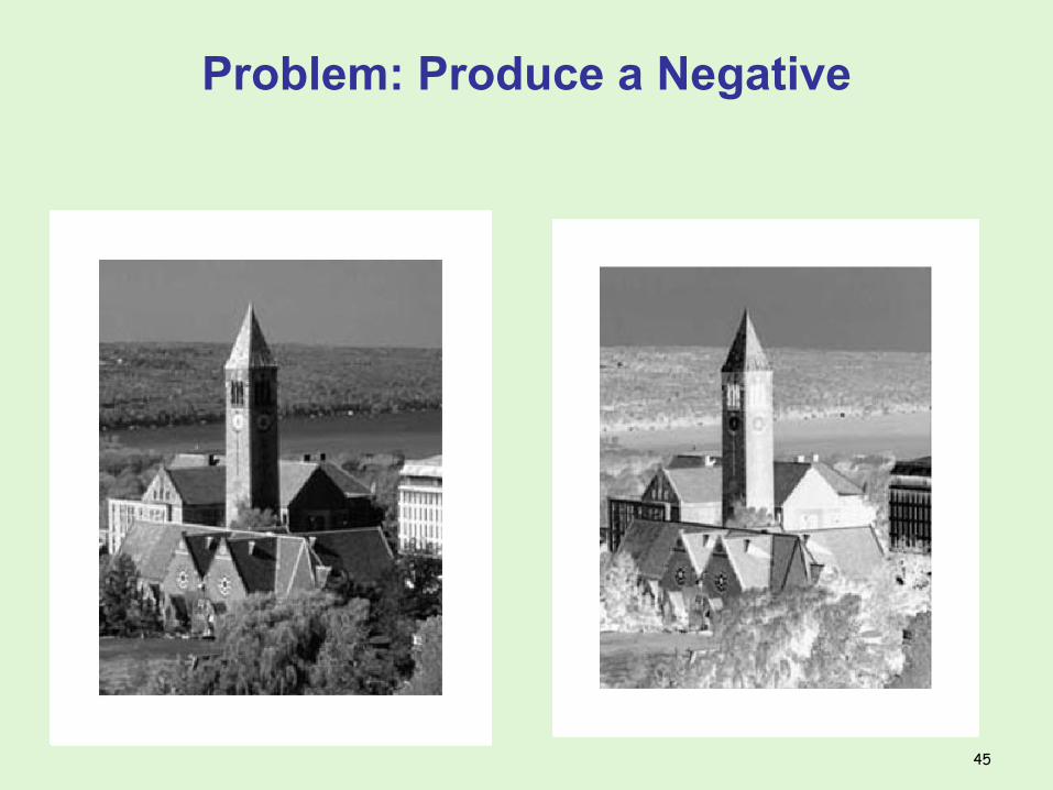
Problem: Produce a Negative

45

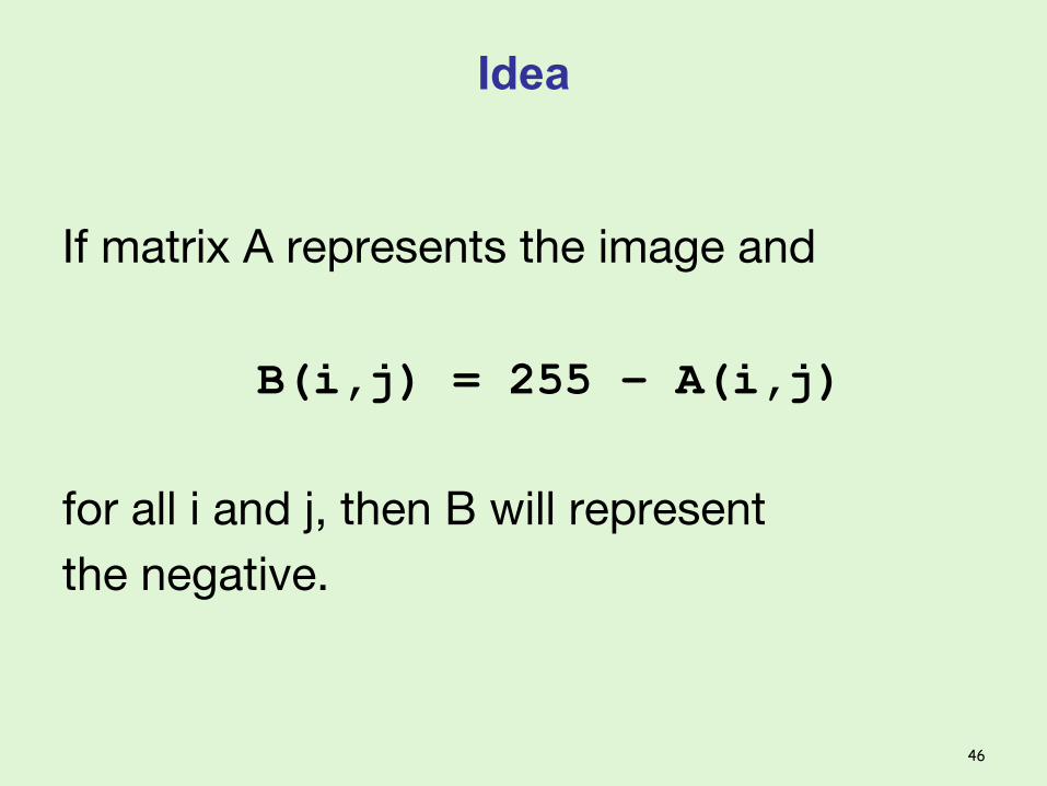
Idea

If matrix A represents the image and B(i,j) = 255 – A(i,j)

for all i and j, then B will representthe negative.

46

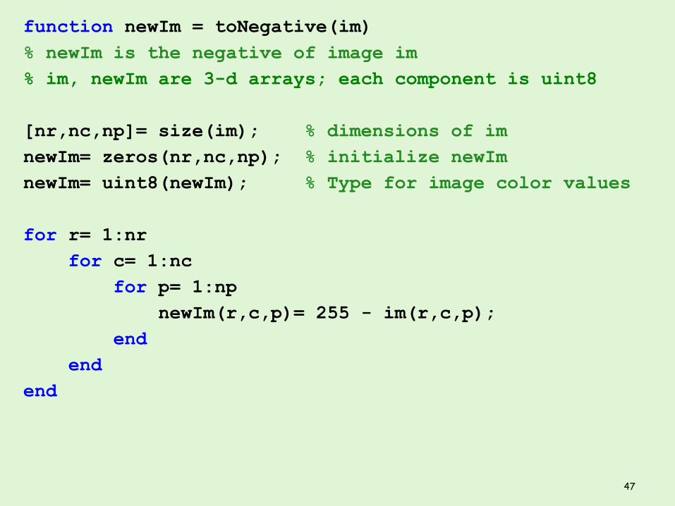
function newIm = toNegative(im)% newIm is the negative of image im% im, newIm are 3-d arrays; each component is uint8 [nr,nc,np]= size(im); % dimensions of imnewIm= zeros(nr,nc,np); % initialize newImnewIm= uint8(newIm); % Type for image color values for r= 1:nr for c= 1:nc for p= 1:np newIm(r,c,p)= 255 - im(r,c,p); end endend

47

Vectorized toNegative

function newIm = toNegative(im)

% newIm is the negative of image im

% im, newIm are 3-d arrays

newIm = 255-im;

48

This is cleaner, clearer, and less error prone.But, always keep complexity in mind.

Previous operations were all element-wise, now we’ll look at some region based operations

Filtering Noise

Edge Detection

49

Working with Images

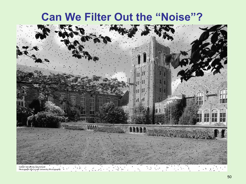
Can We Filter Out the “Noise”?

50

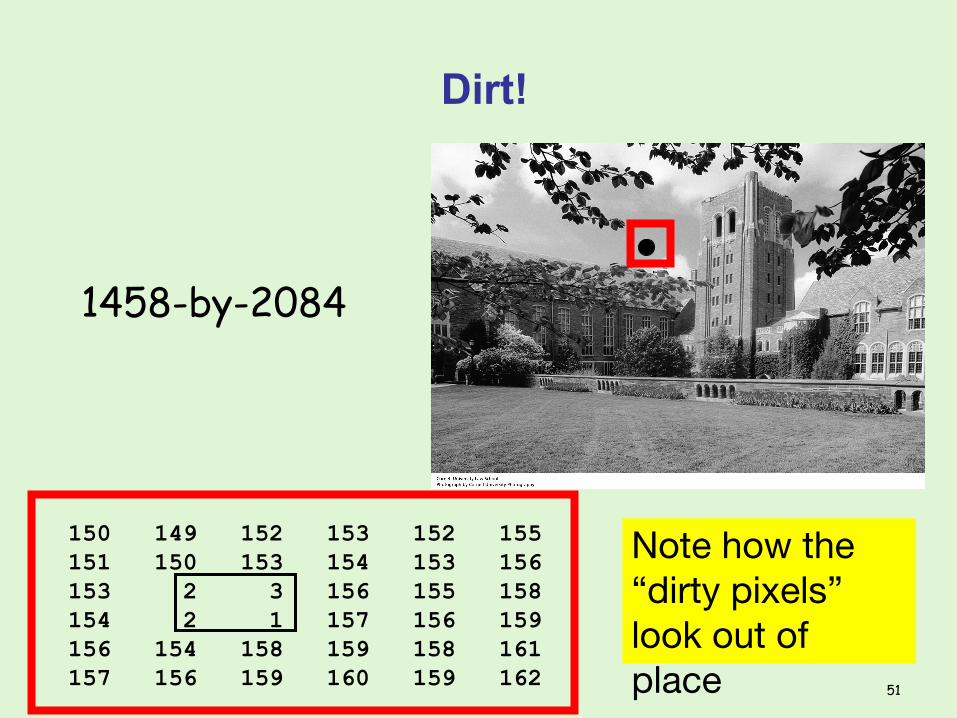
1458-by-2084

150 149 152 153 152 155 151 150 153 154 153 156 153 2 3 156 155 158 154 2 1 157 156 159 156 154 158 159 158 161 157 156 159 160 159 162

Dirt!

Note how the“dirty pixels”look out of place 51

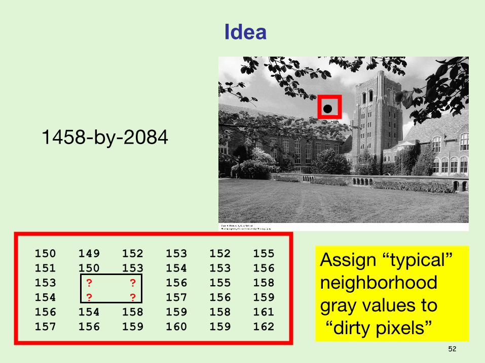
1458-by-2084

150 149 152 153 152 155 151 150 153 154 153 156 153 ? ? 156 155 158 154 ? ? 157 156 159 156 154 158 159 158 161 157 156 159 160 159 162

Idea

Assign “typical”neighborhoodgray values to “dirty pixels”

52

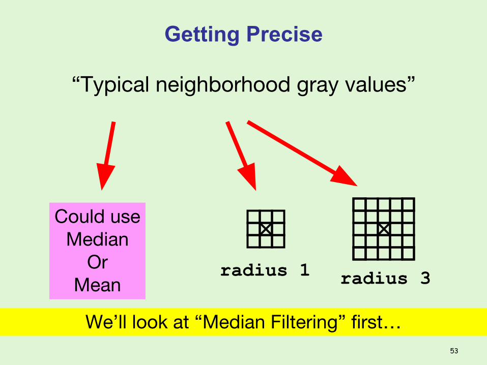
Getting Precise

“Typical neighborhood gray values”

Could useMedian

Or Mean

radius 1 radius 3

We’ll look at “Median Filtering” first…53

Median Filtering

At each pixel, replace its gray value by the median of the gray values in the “neighborhood” i.e. a small region surrounding the pixel.

54

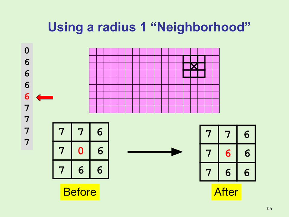
Using a radius 1 “Neighborhood”

6

7

6

7

6

7

7

6

6

6

7

6

7

0

7

7

6

6

Before After

066667777

55

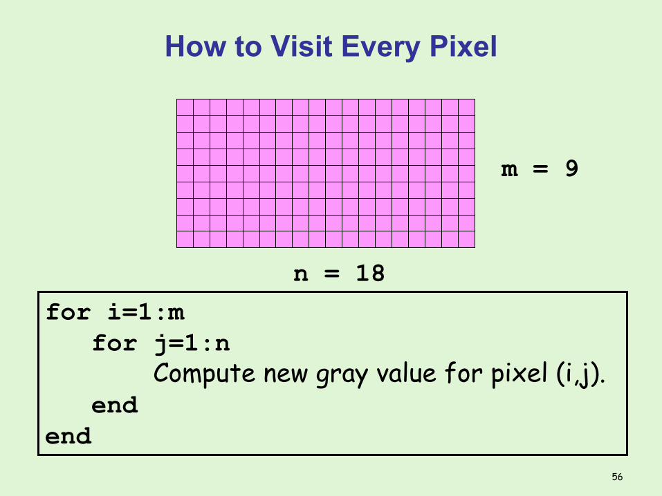
How to Visit Every Pixel

m = 9

n = 18

for i=1:m for j=1:n Compute new gray value for pixel (i,j). endend

56

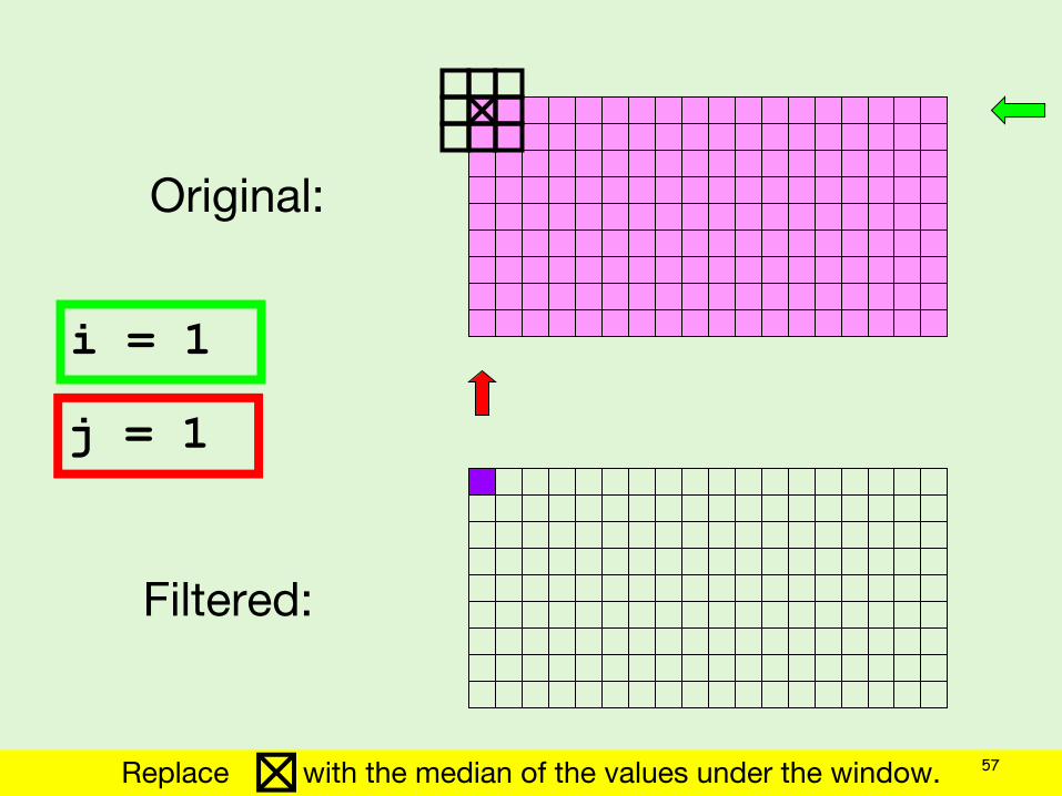
i = 1

j = 1

Original:

Filtered:

Replace with the median of the values under the window. 57

i = 1

j = 2

Original:

Filtered:


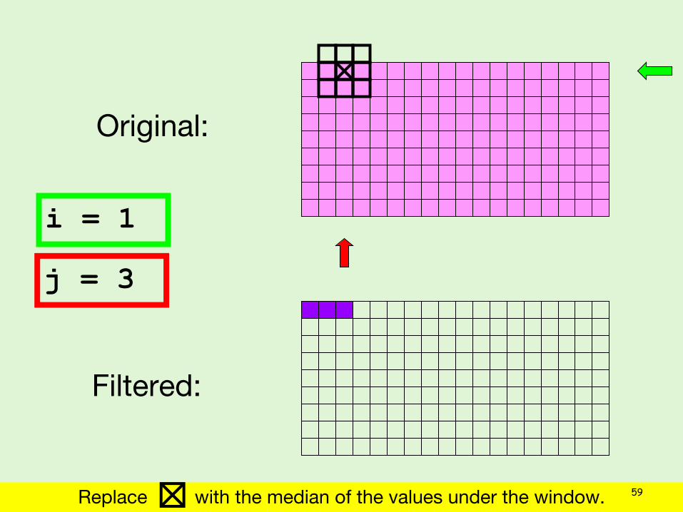
i = 1

j = 3

Original:

Filtered:


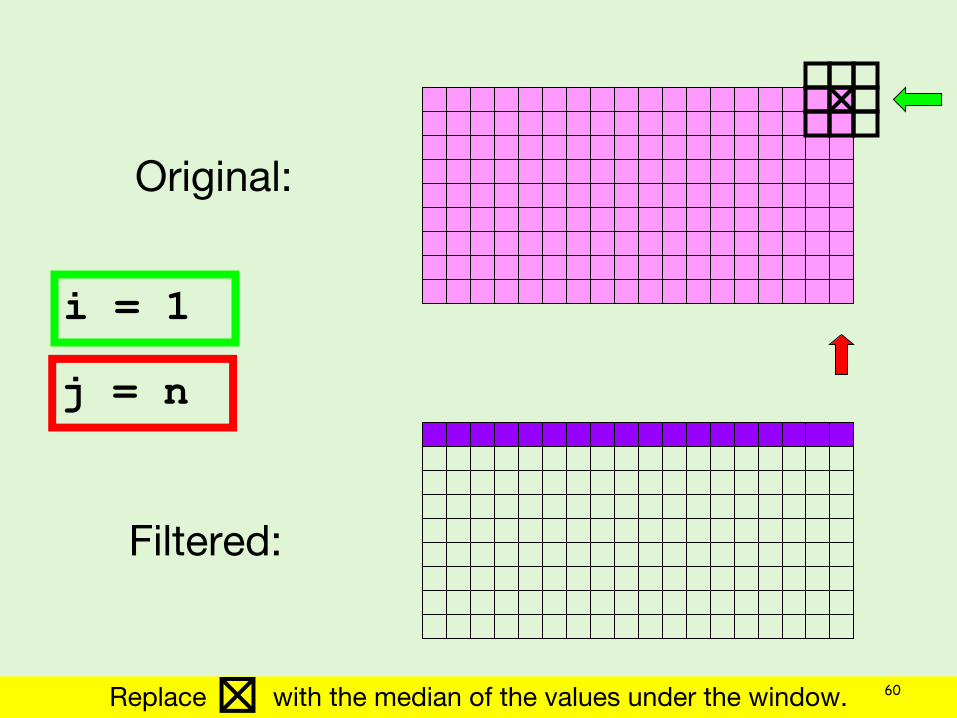
i = 1

j = n

Original:

Filtered:


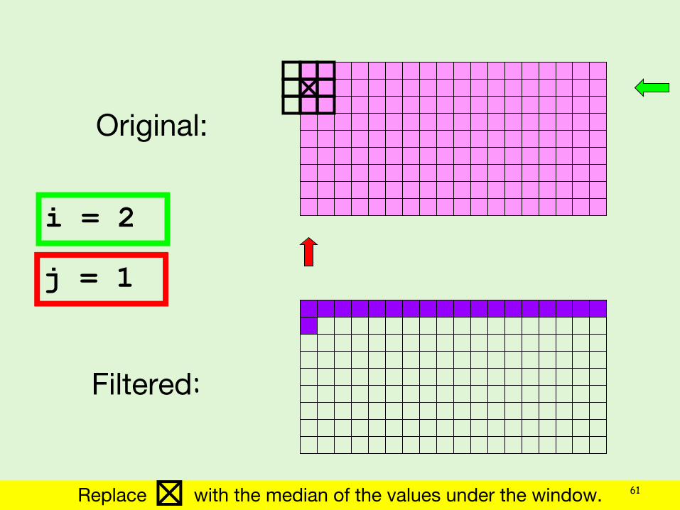
i = 2

j = 1

Original:

Filtered:


i = 2

j = 2

Original:

Filtered:


i = m

j = n

Original:

Filtered:


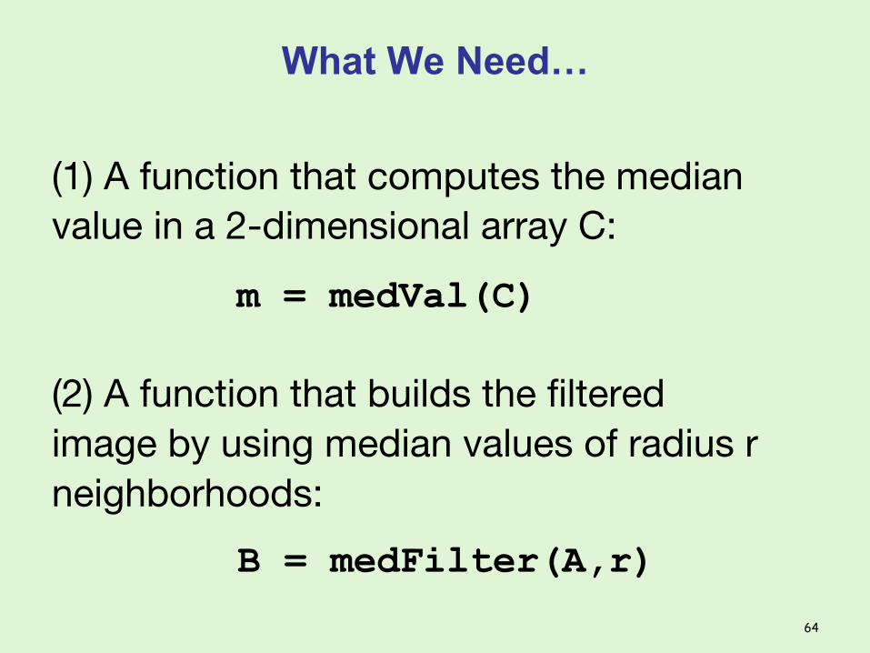
What We Need…

(1) A function that computes the medianvalue in a 2-dimensional array C:

m = medVal(C)

(2) A function that builds the filteredimage by using median values of radius rneighborhoods:

B = medFilter(A,r)

64

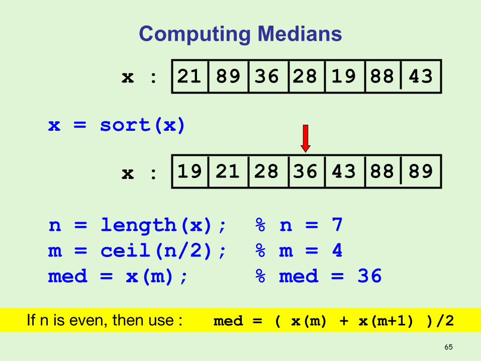
Computing Medians

21 89 36 28 19 88 43x :

x = sort(x)

19 21 28 36 43 88 89x :

n = length(x); % n = 7m = ceil(n/2); % m = 4med = x(m); % med = 36

If n is even, then use : med = ( x(m) + x(m+1) )/2

65

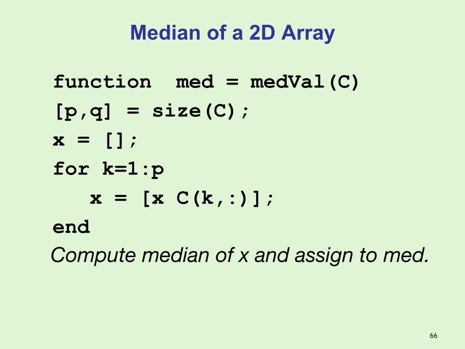
Median of a 2D Array

function med = medVal(C) [p,q] = size(C); x = []; for k=1:p x = [x C(k,:)]; end Compute median of x and assign to med.

66

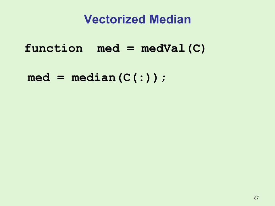
Vectorized Median

67

function med = medVal(C)

med = median(C(:));

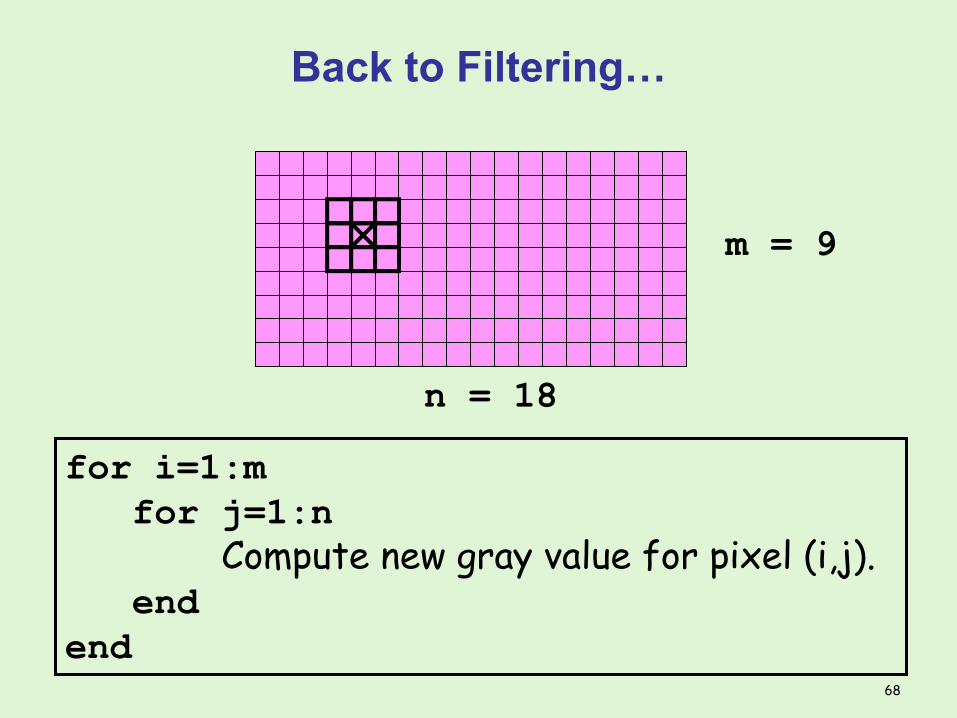
Back to Filtering…

m = 9

n = 18

for i=1:m for j=1:n Compute new gray value for pixel (i,j). endend

68

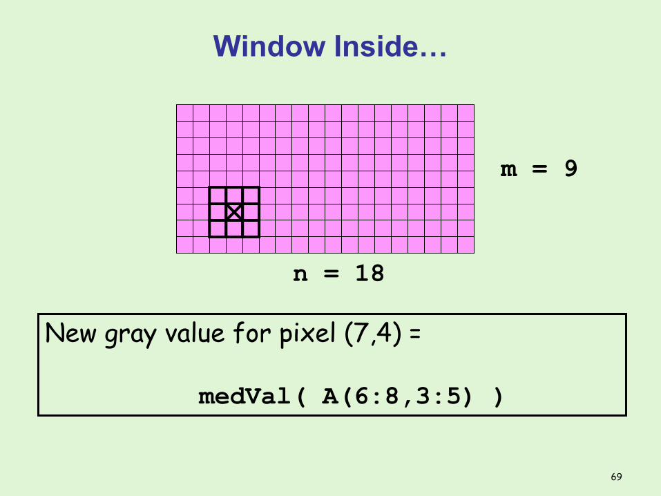
Window Inside…

m = 9

n = 18

New gray value for pixel (7,4) = medVal( A(6:8,3:5) )

69

Window Partly Outside…

m = 9

n = 18


70

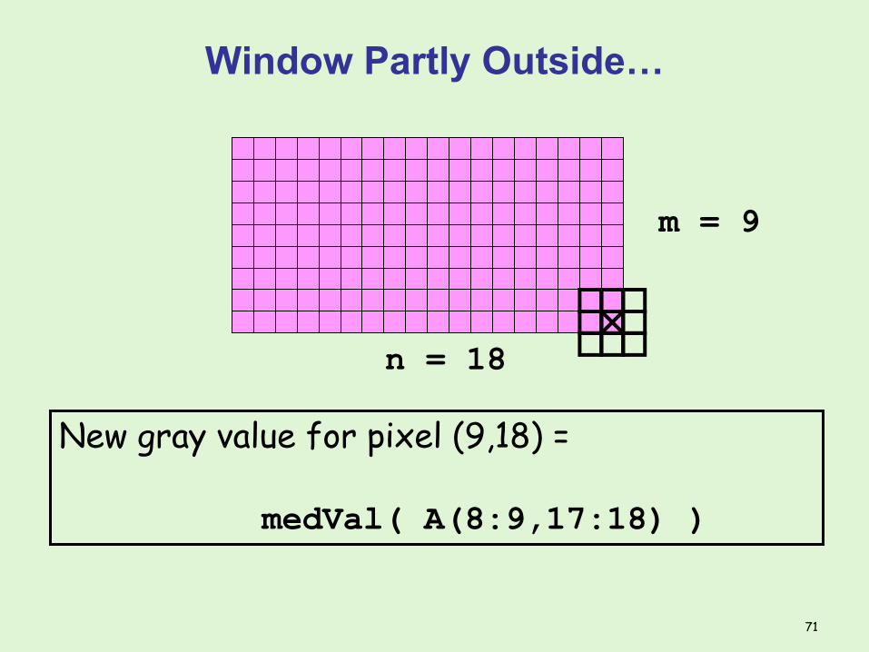
Window Partly Outside…

m = 9

n = 18


71

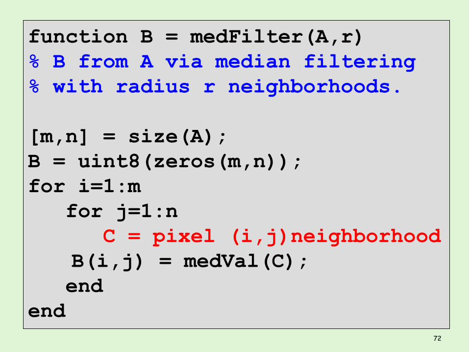
function B = medFilter(A,r) % B from A via median filtering % with radius r neighborhoods. [m,n] = size(A);B = uint8(zeros(m,n));for i=1:m for j=1:n C = pixel (i,j)neighborhood B(i,j) = medVal(C); endend

72

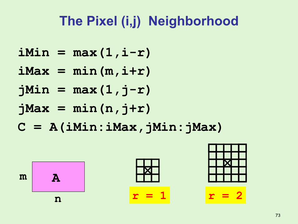
The Pixel (i,j) Neighborhood

iMin = max(1,i-r)iMax = min(m,i+r)jMin = max(1,j-r)jMax = min(n,j+r)C = A(iMin:iMax,jMin:jMax)

r = 1 r = 2

Am

n73

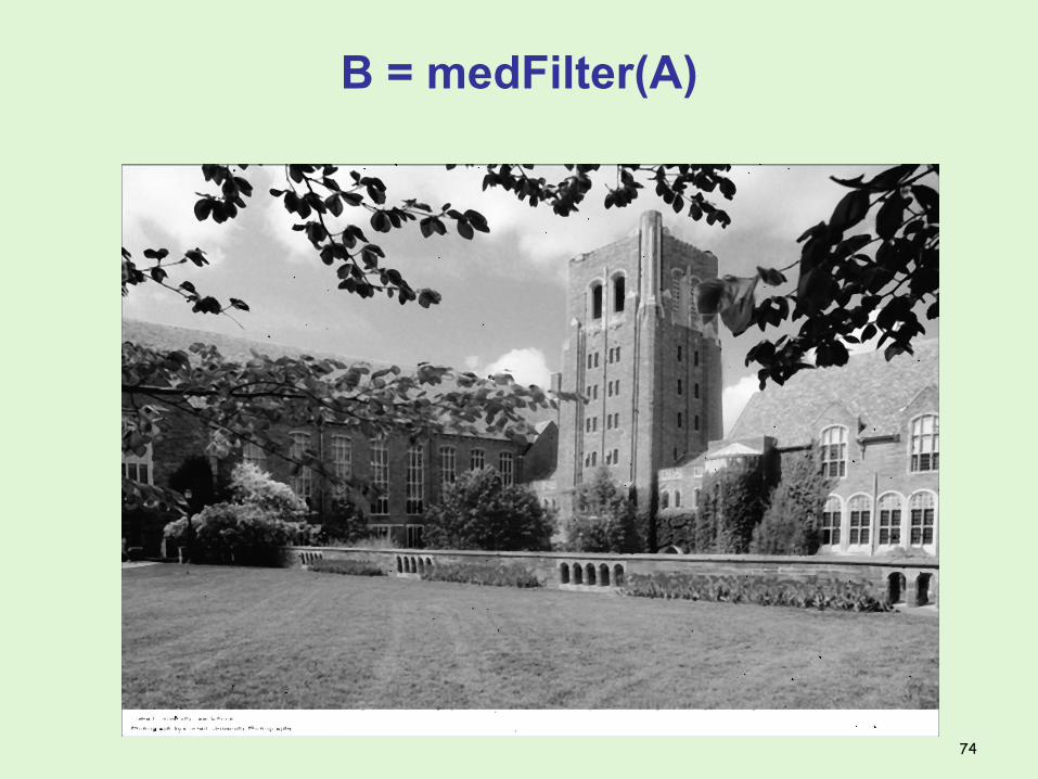
B = medFilter(A)

74

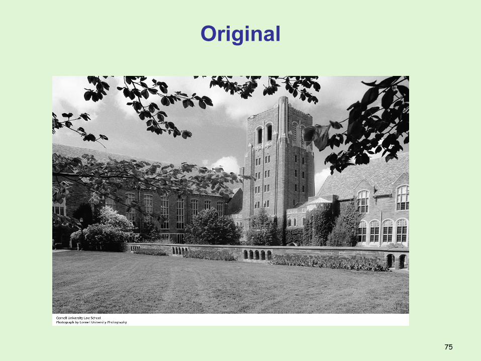
Original

75

What About Using the Meaninstead of the Median?

Replace each gray value with theaverage gray value in the radius rneighborhood.

76

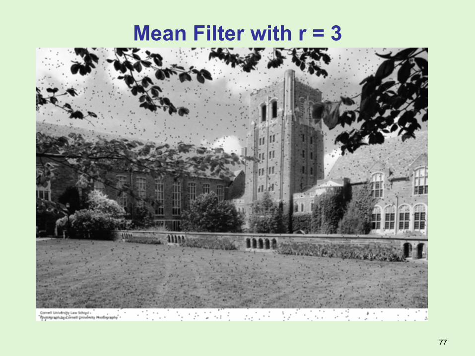
Mean Filter with r = 3

77

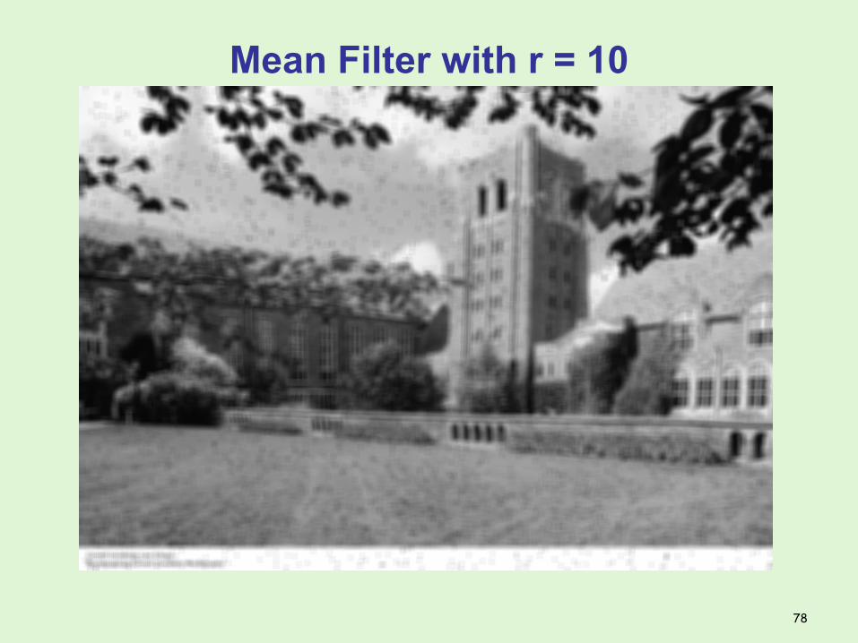
Mean Filter with r = 10

78

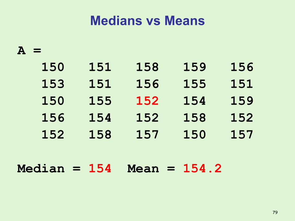
Medians vs Means

A = 150 151 158 159 156 153 151 156 155 151 150 155 152 154 159 156 154 152 158 152 152 158 157 150 157

Median = 154 Mean = 154.2

79

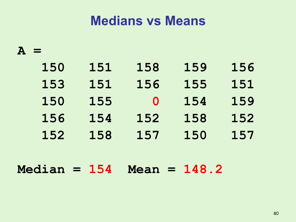
Medians vs Means

A = 150 151 158 159 156 153 151 156 155 151 150 155 0 154 159 156 154 152 158 152 152 158 157 150 157

Median = 154 Mean = 148.2

80

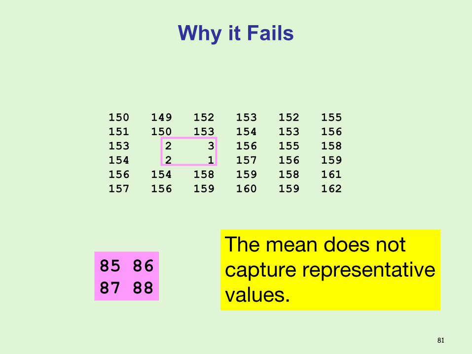
Why it Fails

150 149 152 153 152 155 151 150 153 154 153 156 153 2 3 156 155 158 154 2 1 157 156 159 156 154 158 159 158 161 157 156 159 160 159 162

85 8687 88

The mean does notcapture representativevalues.

81

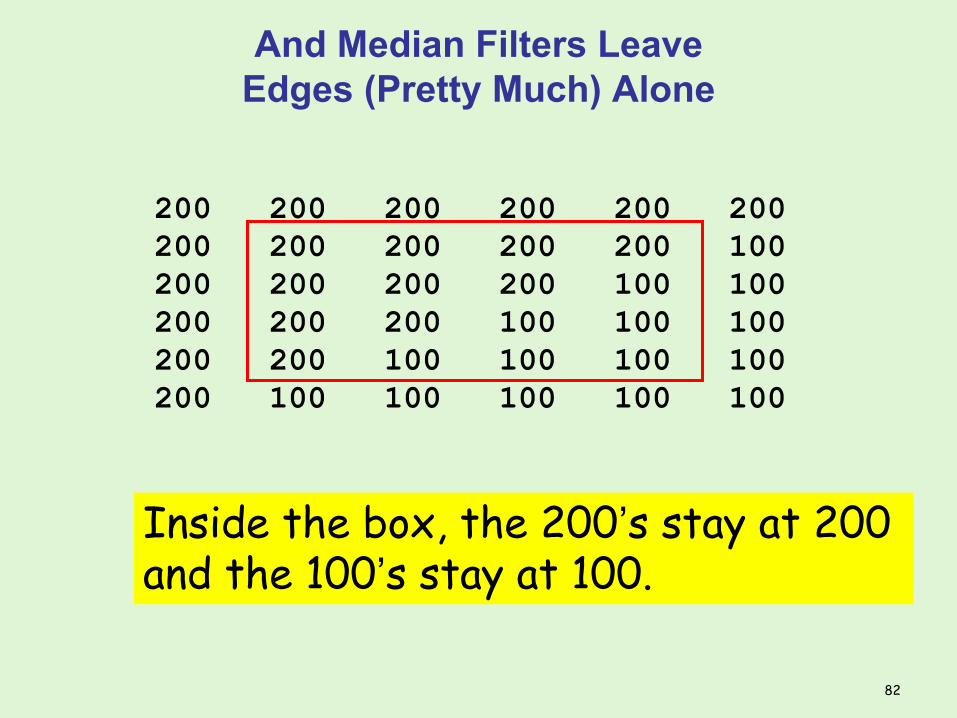
And Median Filters LeaveEdges (Pretty Much) Alone

200 200 200 200 200 200 200 200 200 200 200 100 200 200 200 200 100 100 200 200 200 100 100 100 200 200 100 100 100 100 200 100 100 100 100 100

Inside the box, the 200’s stay at 200 and the 100’s stay at 100.

82

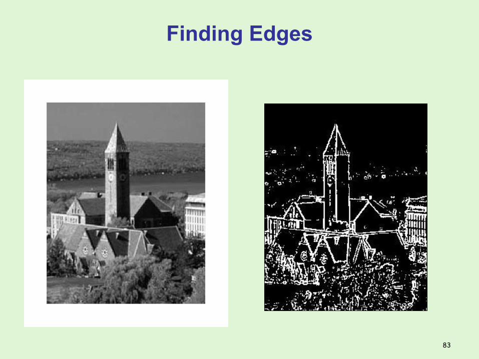
Finding Edges

83

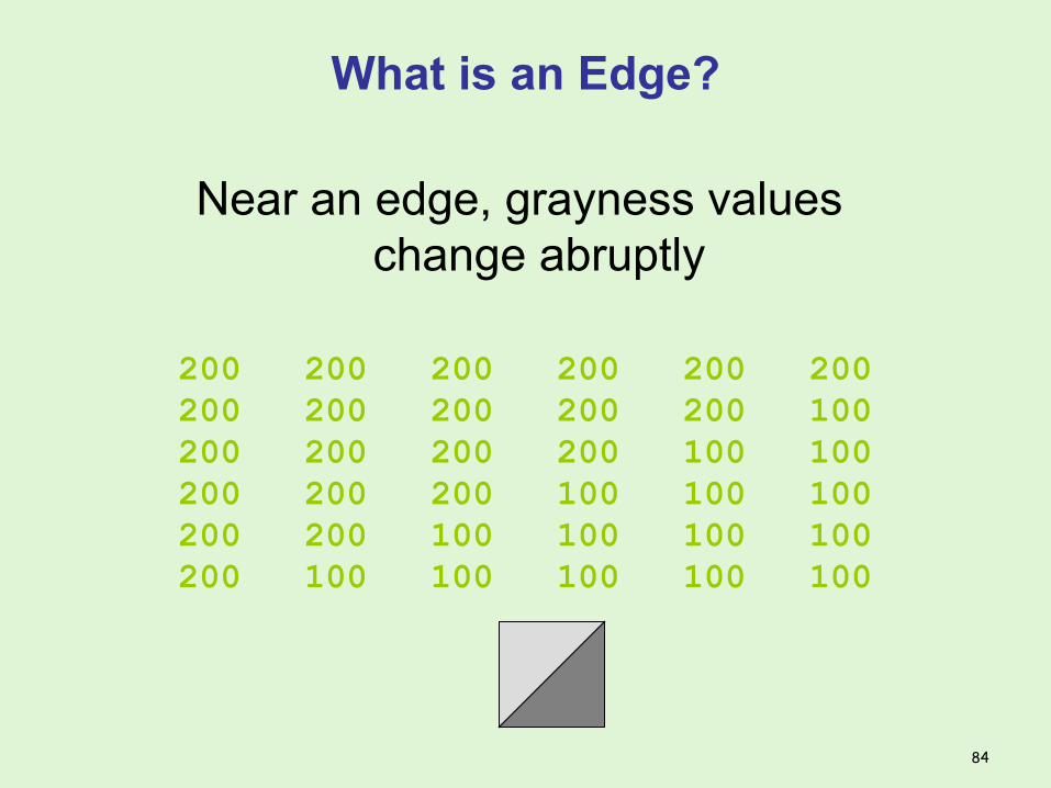
What is an Edge?

Near an edge, grayness values change abruptly

200 200 200 200 200 200 200 200 200 200 200 100 200 200 200 200 100 100 200 200 200 100 100 100 200 200 100 100 100 100 200 100 100 100 100 100

84

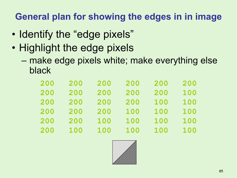
General plan for showing the edges in in image

• Identify the “edge pixels”• Highlight the edge pixels

– make edge pixels white; make everything else black 200 200 200 200 200 200 200 200 200 200 200 100 200 200 200 200 100 100 200 200 200 100 100 100 200 200 100 100 100 100 200 100 100 100 100 100

85

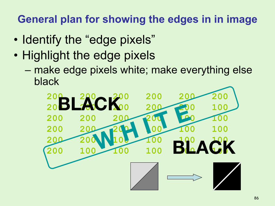
General plan for showing the edges in in image

• Identify the “edge pixels”• Highlight the edge pixels

– make edge pixels white; make everything else black 200 200 200 200 200 200 200 200 200 200 200 100 200 200 200 200 100 100 200 200 200 100 100 100 200 200 100 100 100 100 200 100 100 100 100 100W H I T E

BLACK

BLACK

86

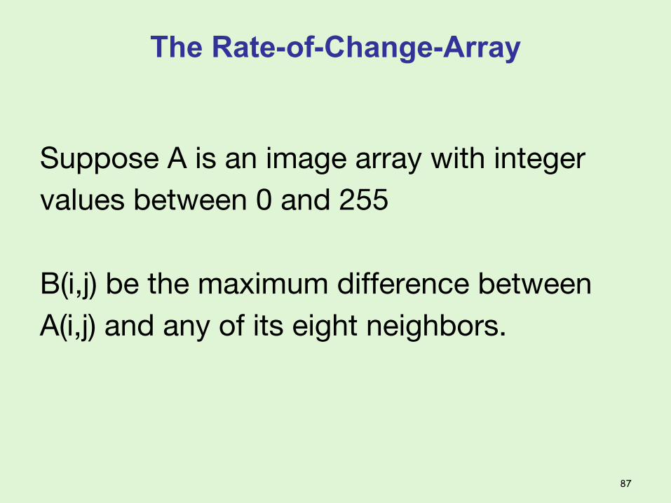
The Rate-of-Change-Array

Suppose A is an image array with integervalues between 0 and 255

B(i,j) be the maximum difference betweenA(i,j) and any of its eight neighbors.

87

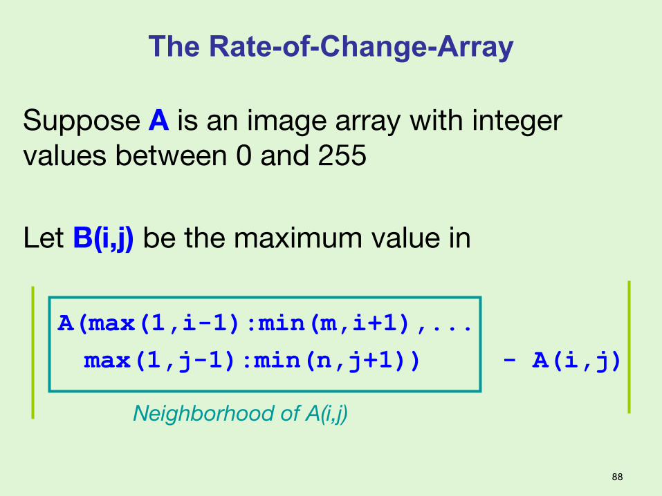
The Rate-of-Change-Array

Suppose A is an image array with integer values between 0 and 255

Let B(i,j) be the maximum value in

A(max(1,i-1):min(m,i+1),... max(1,j-1):min(n,j+1)) - A(i,j)

Neighborhood of A(i,j)

88

Rate-of-change example

59

90

58

60

56

62

65

57

81Rate-of-change at middle pixel is 30

Be careful! In “uint8 arithmetic”

57 – 60 is 0

89

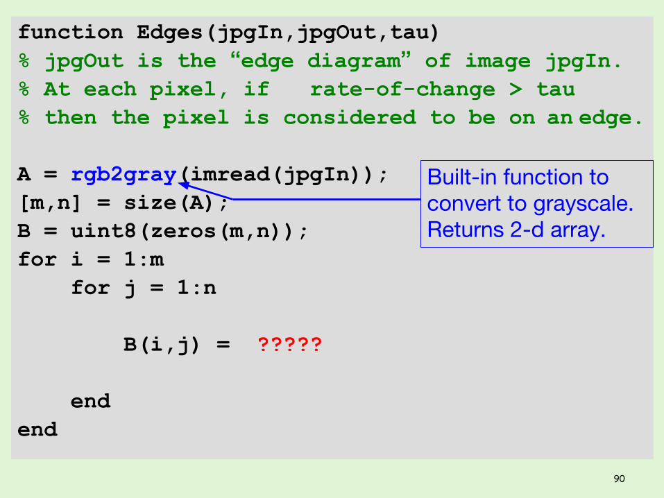
function Edges(jpgIn,jpgOut,tau)% jpgOut is the “edge diagram” of image jpgIn.% At each pixel, if rate-of-change > tau% then the pixel is considered to be on an edge.

A = rgb2gray(imread(jpgIn));[m,n] = size(A);B = uint8(zeros(m,n));for i = 1:m for j = 1:n

B(i,j) = ?????

endend

Built-in function to convert to grayscale. Returns 2-d array.

90

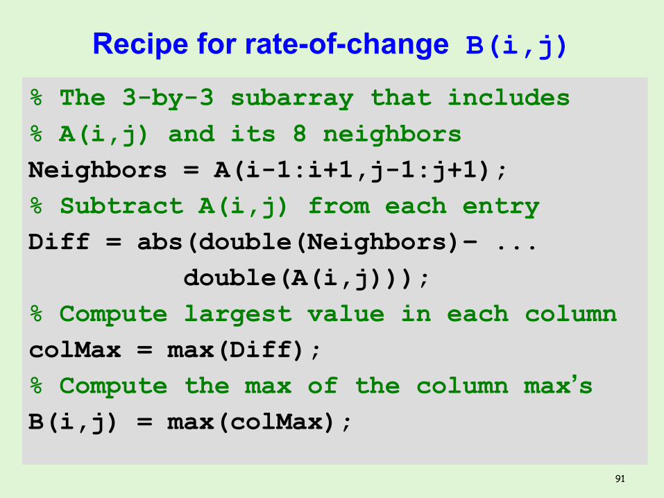
Recipe for rate-of-change B(i,j)% The 3-by-3 subarray that includes% A(i,j) and its 8 neighborsNeighbors = A(i-1:i+1,j-1:j+1);% Subtract A(i,j) from each entryDiff = abs(double(Neighbors)– ... double(A(i,j)));% Compute largest value in each columncolMax = max(Diff);% Compute the max of the column max’sB(i,j) = max(colMax);

91


A = rgb2gray(imread(jpgIn));[m,n] = size(A);B = uint8(zeros(m,n));for i = 1:m for j = 1:n

B(i,j) = ?????

endend

92


A = rgb2gray(imread(jpgIn));[m,n] = size(A);B = uint8(zeros(m,n));for i = 1:m for j = 1:n Neighbors = A(max(1,i-1):min(i+1,m), ... max(1,j-1):min(j+1,n)); B(i,j)=max(max(abs(double(Neighbors)– ... double(A(i,j))))); endend

93

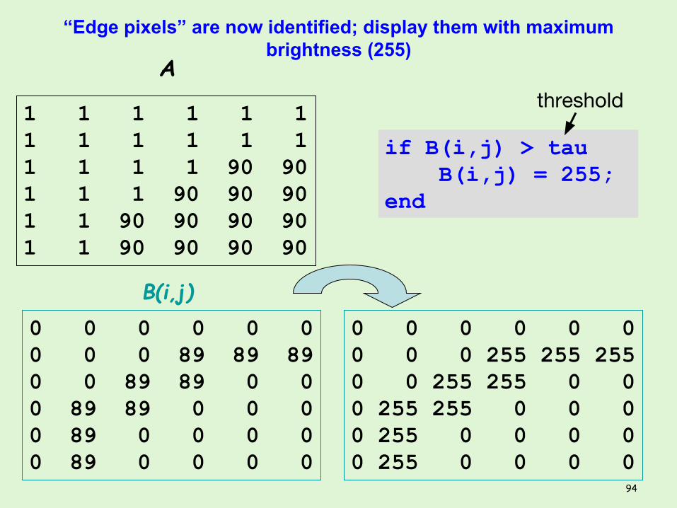
“Edge pixels” are now identified; display them with maximum brightness (255)

1 1 1 1 1 11 1 1 1 1 11 1 1 1 90 901 1 1 90 90 901 1 90 90 90 901 1 90 90 90 90

0 0 0 0 0 00 0 0 89 89 890 0 89 89 0 00 89 89 0 0 00 89 0 0 0 00 89 0 0 0 0

A

B(i,j)0 0 0 0 0 00 0 0 255 255 2550 0 255 255 0 00 255 255 0 0 00 255 0 0 0 00 255 0 0 0 0

if B(i,j) > tau B(i,j) = 255;end

threshold

94

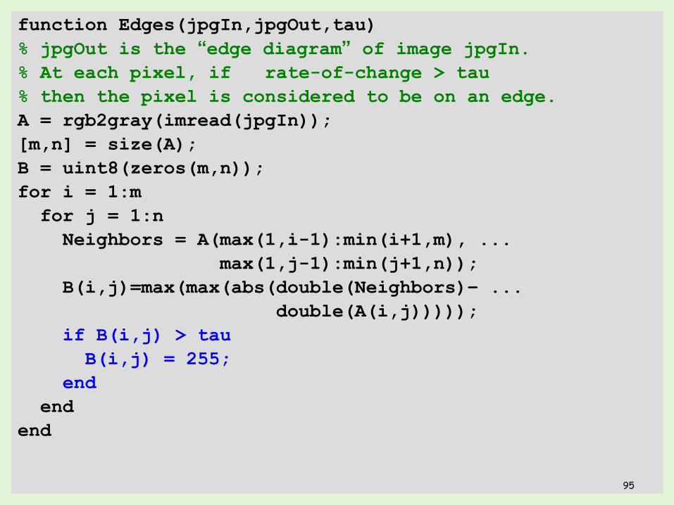
function Edges(jpgIn,jpgOut,tau)% jpgOut is the “edge diagram” of image jpgIn.% At each pixel, if rate-of-change > tau% then the pixel is considered to be on an edge.A = rgb2gray(imread(jpgIn));[m,n] = size(A);B = uint8(zeros(m,n));for i = 1:m for j = 1:n Neighbors = A(max(1,i-1):min(i+1,m), ... max(1,j-1):min(j+1,n)); B(i,j)=max(max(abs(double(Neighbors)– ... double(A(i,j))))); if B(i,j) > tau B(i,j) = 255; end endend

95

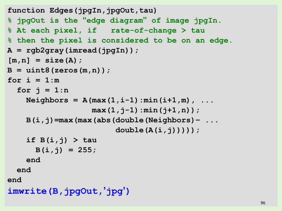
function Edges(jpgIn,jpgOut,tau)% jpgOut is the “edge diagram” of image jpgIn.% At each pixel, if rate-of-change > tau% then the pixel is considered to be on an edge.A = rgb2gray(imread(jpgIn));[m,n] = size(A);B = uint8(zeros(m,n));for i = 1:m for j = 1:n Neighbors = A(max(1,i-1):min(i+1,m), ... max(1,j-1):min(j+1,n)); B(i,j)=max(max(abs(double(Neighbors)– ... double(A(i,j))))); if B(i,j) > tau B(i,j) = 255; end endend

imwrite(B,jpgOut,’jpg’)96

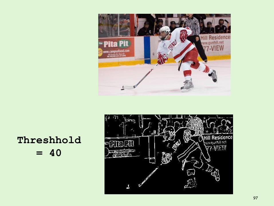
Threshhold = 40

97

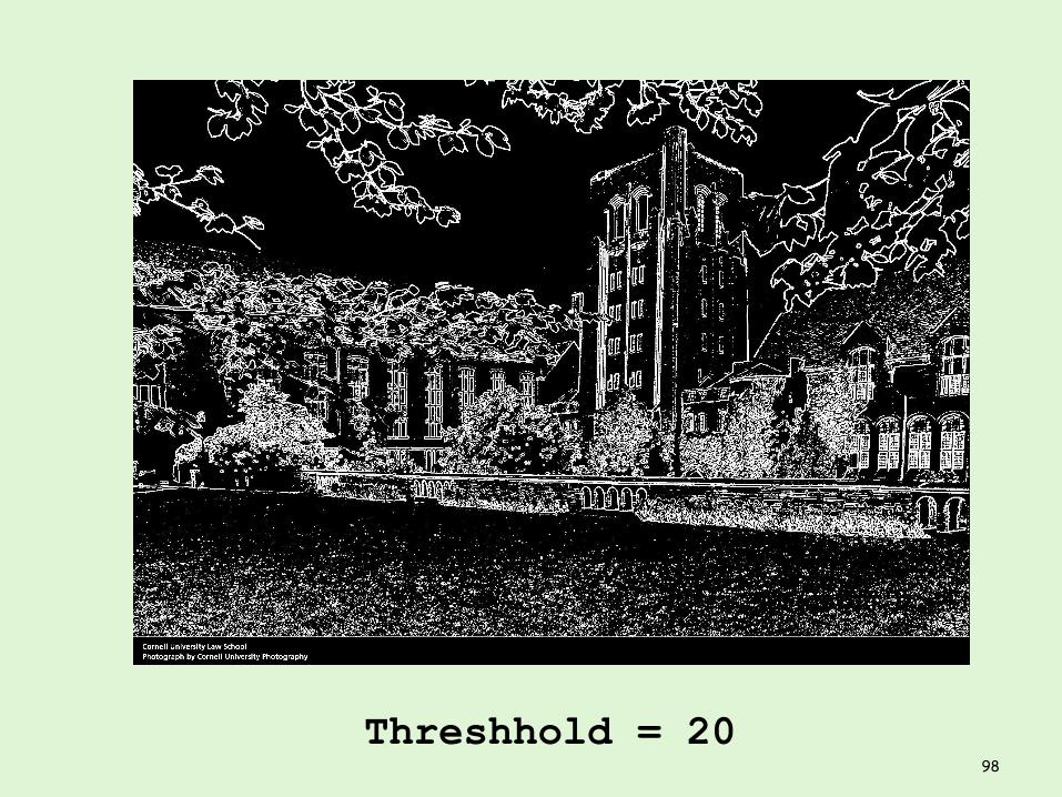
Threshhold = 2098

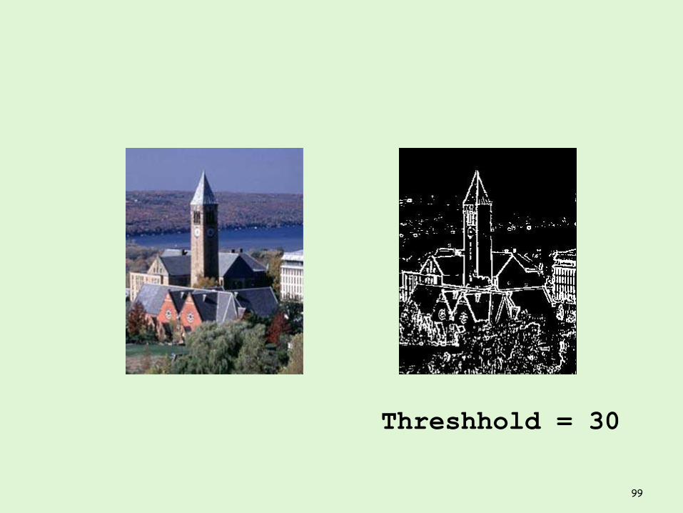
Threshhold = 30

99

Documents

Lecture 19 Image processing - cs.brown.edu