Embed Size (px)
Citation preview
Version 2.3 © 1995-2007 I.T. Young, J.J. Gerbrands and L.J. van Vliet 1
Fundamentals of Image Processing
1. Introduction ..............................................1 2. Digital Image Definitions.........................2 3. Tools.........................................................6 4. Perception...............................................22 5. Image Sampling......................................28 6. Noise.......................................................32 7. Cameras ..................................................35 8. Displays..................................................44 Ian T. Young 9. Algorithms..............................................44 Jan J. Gerbrands 10. Techniques .............................................86 Lucas J. van Vliet 11. Acknowledgments ................................109 Delft University of Technology 12. References ............................................109
1. Introduction Modern digital technology has made it possible to manipulate multi-dimensional signals with systems that range from simple digital circuits to advanced parallel computers. The goal of this manipulation can be divided into three categories: • Image Processing image in → image out • Image Analysis image in → measurements out • Image Understanding image in → high-level description out We will focus on the fundamental concepts of image processing. Space does not permit us to make more than a few introductory remarks about image analysis. Image understanding requires an approach that differs fundamentally from the theme of this book. Further, we will restrict ourselves to two–dimensional (2D) image processing although most of the concepts and techniques that are to be described can be extended easily to three or more dimensions. Readers interested in either greater detail than presented here or in other aspects of image processing are referred to [1-10]
…Image Processing Fundamentals
2
We begin with certain basic definitions. An image defined in the “real world” is considered to be a function of two real variables, for example, a(x,y) with a as the amplitude (e.g. brightness) of the image at the real coordinate position (x,y). An image may be considered to contain sub-images sometimes referred to as regions–of–interest, ROIs, or simply regions. This concept reflects the fact that images frequently contain collections of objects each of which can be the basis for a region. In a sophisticated image processing system it should be possible to apply specific image processing operations to selected regions. Thus one part of an image (region) might be processed to suppress motion blur while another part might be processed to improve color rendition. The amplitudes of a given image will almost always be either real numbers or integer numbers. The latter is usually a result of a quantization process that converts a continuous range (say, between 0 and 100%) to a discrete number of levels. In certain image-forming processes, however, the signal may involve photon counting which implies that the amplitude would be inherently quantized. In other image forming procedures, such as magnetic resonance imaging, the direct physical measurement yields a complex number in the form of a real magnitude and a real phase. For the remainder of this book we will consider amplitudes as reals or integers unless otherwise indicated.
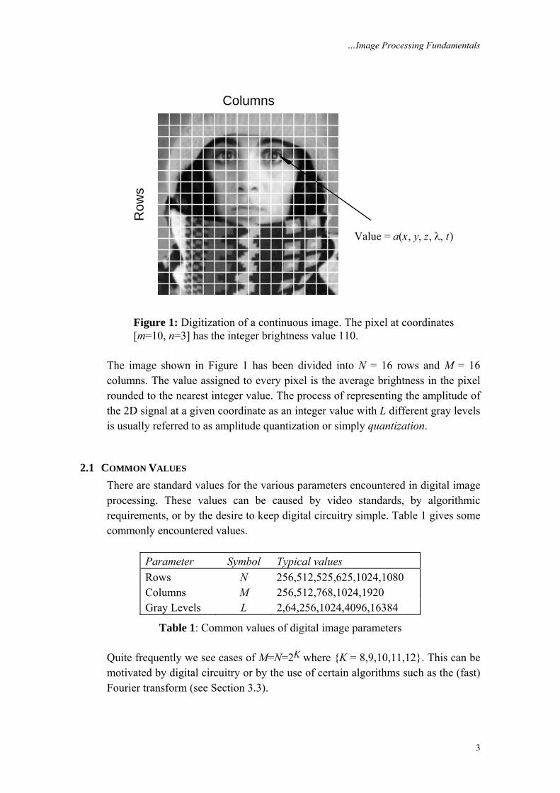
2. Digital Image Definitions A digital image a[m,n] described in a 2D discrete space is derived from an analog image a(x,y) in a 2D continuous space through a sampling process that is frequently referred to as digitization. The mathematics of that sampling process will be described in Section 5. For now we will look at some basic definitions associated with the digital image. The effect of digitization is shown in Figure 1. The 2D continuous image a(x,y) is divided into N rows and M columns. The intersection of a row and a column is termed a pixel. The value assigned to the integer coordinates [m,n] with {m=0,1,2,…,M–1} and {n=0,1,2,…,N–1} is a[m,n]. In fact, in most cases a(x,y) – which we might consider to be the physical signal that impinges on the face of a 2D sensor – is actually a function of many variables including depth (z), color (λ), and time (t). Unless otherwise stated, we will consider the case of 2D, monochromatic, static images in this chapter.
…Image Processing Fundamentals
3
Row
s
Columns
Value = a(x, y, z, λ, t)
Figure 1: Digitization of a continuous image. The pixel at coordinates [m=10, n=3] has the integer brightness value 110.
The image shown in Figure 1 has been divided into N = 16 rows and M = 16 columns. The value assigned to every pixel is the average brightness in the pixel rounded to the nearest integer value. The process of representing the amplitude of the 2D signal at a given coordinate as an integer value with L different gray levels is usually referred to as amplitude quantization or simply quantization.
2.1 COMMON VALUES There are standard values for the various parameters encountered in digital image processing. These values can be caused by video standards, by algorithmic requirements, or by the desire to keep digital circuitry simple. Table 1 gives some commonly encountered values.
Parameter Symbol Typical values Rows N 256,512,525,625,1024,1080 Columns M 256,512,768,1024,1920 Gray Levels L 2,64,256,1024,4096,16384
Table 1: Common values of digital image parameters Quite frequently we see cases of M=N=2K where {K = 8,9,10,11,12}. This can be motivated by digital circuitry or by the use of certain algorithms such as the (fast) Fourier transform (see Section 3.3).
…Image Processing Fundamentals
4
The number of distinct gray levels is usually a power of 2, that is, L=2B where B is the number of bits in the binary representation of the brightness levels. When B>1 we speak of a gray-level image; when B=1 we speak of a binary image. In a binary image there are just two gray levels which can be referred to, for example, as “black” and “white” or “0” and “1”.
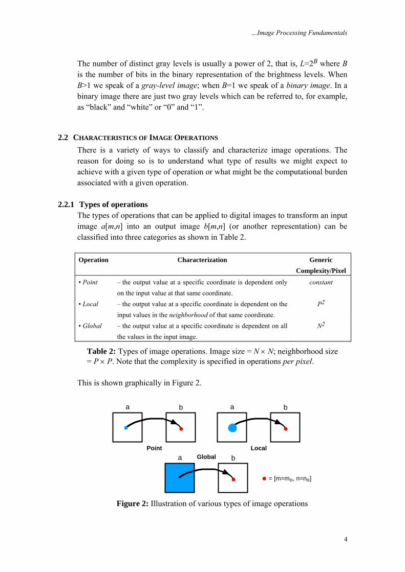
2.2 CHARACTERISTICS OF IMAGE OPERATIONS There is a variety of ways to classify and characterize image operations. The reason for doing so is to understand what type of results we might expect to achieve with a given type of operation or what might be the computational burden associated with a given operation.
2.2.1 Types of operations The types of operations that can be applied to digital images to transform an input image a[m,n] into an output image b[m,n] (or another representation) can be classified into three categories as shown in Table 2. Operation Characterization Generic
Complexity/Pixel
• Point – the output value at a specific coordinate is dependent only on the input value at that same coordinate.
constant
• Local – the output value at a specific coordinate is dependent on the input values in the neighborhood of that same coordinate.
P2
• Global – the output value at a specific coordinate is dependent on all the values in the input image.
N2
Table 2: Types of image operations. Image size = N × N; neighborhood size = P × P. Note that the complexity is specified in operations per pixel.
This is shown graphically in Figure 2.
a b
Point
a b
Locala bGlobal
= [m=mo, n=no]
Figure 2: Illustration of various types of image operations
…Image Processing Fundamentals
5
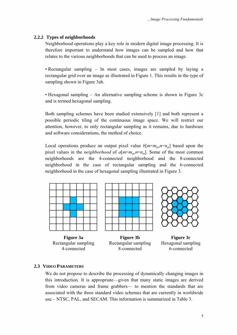
2.2.2 Types of neighborhoods Neighborhood operations play a key role in modern digital image processing. It is therefore important to understand how images can be sampled and how that relates to the various neighborhoods that can be used to process an image. • Rectangular sampling – In most cases, images are sampled by laying a rectangular grid over an image as illustrated in Figure 1. This results in the type of sampling shown in Figure 3ab. • Hexagonal sampling – An alternative sampling scheme is shown in Figure 3c and is termed hexagonal sampling. Both sampling schemes have been studied extensively [1] and both represent a possible periodic tiling of the continuous image space. We will restrict our attention, however, to only rectangular sampling as it remains, due to hardware and software considerations, the method of choice. Local operations produce an output pixel value b[m=mo,n=no] based upon the pixel values in the neighborhood of a[m=mo,n=no]. Some of the most common neighborhoods are the 4-connected neighborhood and the 8-connected neighborhood in the case of rectangular sampling and the 6-connected neighborhood in the case of hexagonal sampling illustrated in Figure 3.
Figure 3a Figure 3b Figure 3c Rectangular sampling Rectangular sampling Hexagonal sampling 4-connected 8-connected 6-connected
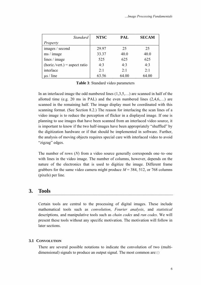
2.3 VIDEO PARAMETERS We do not propose to describe the processing of dynamically changing images in this introduction. It is appropriate—given that many static images are derived from video cameras and frame grabbers— to mention the standards that are associated with the three standard video schemes that are currently in worldwide use – NTSC, PAL, and SECAM. This information is summarized in Table 3.
…Image Processing Fundamentals
6
Standard NTSC PAL SECAM
Property images / second 29.97 25 25 ms / image 33.37 40.0 40.0 lines / image 525 625 625 (horiz./vert.) = aspect ratio 4:3 4:3 4:3 interlace 2:1 2:1 2:1 µs / line 63.56 64.00 64.00
Table 3: Standard video parameters In an interlaced image the odd numbered lines (1,3,5,…) are scanned in half of the allotted time (e.g. 20 ms in PAL) and the even numbered lines (2,4,6,…) are scanned in the remaining half. The image display must be coordinated with this scanning format. (See Section 8.2.) The reason for interlacing the scan lines of a video image is to reduce the perception of flicker in a displayed image. If one is planning to use images that have been scanned from an interlaced video source, it is important to know if the two half-images have been appropriately “shuffled” by the digitization hardware or if that should be implemented in software. Further, the analysis of moving objects requires special care with interlaced video to avoid “zigzag” edges. The number of rows (N) from a video source generally corresponds one–to–one with lines in the video image. The number of columns, however, depends on the nature of the electronics that is used to digitize the image. Different frame grabbers for the same video camera might produce M = 384, 512, or 768 columns (pixels) per line.
3. Tools Certain tools are central to the processing of digital images. These include mathematical tools such as convolution, Fourier analysis, and statistical descriptions, and manipulative tools such as chain codes and run codes. We will present these tools without any specific motivation. The motivation will follow in later sections.
3.1 CONVOLUTION There are several possible notations to indicate the convolution of two (multi-dimensional) signals to produce an output signal. The most common are:
…Image Processing Fundamentals
7
c a b a b= ⊗ = ∗ (1) We shall use the first form, c a b= ⊗ , with the following formal definitions. In 2D continuous space:
( , ) ( , ) ( , ) ( , ) ( , )c x y a x y b x y a b x y d dχ ζ χ ζ χ ζ+∞ +∞
−∞ −∞
= ⊗ = − −∫ ∫ (2)
In 2D discrete space:
[ , ] [ , ] [ , ] [ , ] [ , ]j k
c m n a m n b m n a j k b m j n k+∞ +∞
=−∞ =−∞= ⊗ = − −∑ ∑ (3)
3.2 PROPERTIES OF CONVOLUTION There are a number of important mathematical properties associated with convolution. • Convolution is commutative. c a b b a= ⊗ = ⊗ (4) • Convolution is associative. ( ) ( )c a b d a b d a b d= ⊗ ⊗ = ⊗ ⊗ = ⊗ ⊗ (5) • Convolution is distributive. ( ) ( ) ( )c a b d a b a d= ⊗ + = ⊗ + ⊗ (6) where a, b, c, and d are all images, either continuous or discrete.
3.3 FOURIER TRANSFORMS The Fourier transform produces another representation of a signal, specifically a representation as a weighted sum of complex exponentials. Because of Euler’s formula: cos( ) sin( )jqe q j q= + (7) where 2 1j = − , we can say that the Fourier transform produces a representation of a (2D) signal as a weighted sum of sines and cosines. The defining formulas for
…Image Processing Fundamentals
8
the forward Fourier and the inverse Fourier transforms are as follows. Given an image a and its Fourier transform A, then the forward transform goes from the spatial domain (either continuous or discrete) to the frequency domain which is always continuous. Forward – { }A a=F (8)
The inverse Fourier transform goes from the frequency domain back to the spatial domain. Inverse – { }1a A−=F (9)
The Fourier transform is a unique and invertible operation so that: { }{ } { }{ }1 1a a and A A− −= =F F F F (10)
The specific formulas for transforming back and forth between the spatial domain and the frequency domain are given below. In 2D continuous space:
Forward – ( )( , ) ( , ) j ux vyA u v a x y e dxdy+∞ +∞
− +
−∞ −∞
= ∫ ∫ (11)
Inverse – ( )2
1( , ) ( , )4
j ux vya x y A u v e dudvπ
+∞ +∞+ +
−∞ −∞
= ∫ ∫ (12)
In 2D discrete space:
Forward – ( )( , ) [ , ] j m n
m nA a m n e
+∞ +∞− Ω +Ψ
=−∞ =−∞
Ω Ψ = ∑ ∑ (13)
Inverse – ( )2
1[ , ] ( , )4
j m na m n A e d dπ π
π
+ ++ Ω +Ψ
−π −π
= Ω Ψ Ω Ψ∫ ∫ (14)
3.4 PROPERTIES OF FOURIER TRANSFORMS There are a variety of properties associated with the Fourier transform and the inverse Fourier transform. The following are some of the most relevant for digital image processing.
…Image Processing Fundamentals
9
• The Fourier transform is, in general, a complex function of the real frequency variables. As such the transform can be written in terms of its magnitude and phase. ( , ) ( , )( , ) ( , ) ( , ) ( , )j u v jA u v A u v e A A eϕ ϕ Ω Ψ= Ω Ψ = Ω Ψ (15)
• A 2D signal can also be complex and thus written in terms of its magnitude and phase. ( , ) [ , ]( , ) ( , ) [ , ] [ , ]j x y j m na x y a x y e a m n a m n eϑ ϑ= = (16)
• If a 2D signal is real, then the Fourier transform has certain symmetries. * *( , ) ( , ) ( , ) ( , )A u v A u v A A= − − Ω Ψ = −Ω −Ψ (17) The symbol (*) indicates complex conjugation. For real signals eq. (17) leads directly to:
( , ) ( , ) ( , ) ( , )
( , ) ( , ) ( , ) ( , )
A u v A u v u v u v
A A
ϕ ϕ
ϕ ϕ
= − − = − − −
Ω Ψ = −Ω −Ψ Ω Ψ = − −Ω −Ψ (18)
• If a 2D signal is real and even, then the Fourier transform is real and even. ( , ) ( , ) ( , ) ( , )A u v A u v A A= − − Ω Ψ = −Ω −Ψ (19) • The Fourier and the inverse Fourier transforms are linear operations.
{ } { } { }
{ } { } { }1 2 1 2 1 2
1 1 11 2 1 2 1 2
w a w b w a w b w A w B
w A w B w A w B w a w b− − −
+ = + = +
+ = + = +
F F FF F F
(20)
where a and b are 2D signals (images) and w1 and w2 are arbitrary, complex constants. • The Fourier transform in discrete space, A(Ω,Ψ), is periodic in both Ω and Ψ. Both periods are 2π. ( 2 , 2 ) ( , ) , integersA j k A j kπ πΩ + Ψ + = Ω Ψ (21) • The energy, E, in a signal can be measured either in the spatial domain or the frequency domain. For a signal with finite energy:
…Image Processing Fundamentals
10
Parseval’s theorem (2D continuous space):
2 22
1( , ) ( , )4
E a x y dxdy A u v dudvπ
+∞ +∞ +∞ +∞
−∞ −∞ −∞ −∞
= =∫ ∫ ∫ ∫ (22)
Parseval’s theorem (2D discrete space):
2 22
1[ , ] ( , )4m n
E a m n A d dπ π
π ππ
+ ++∞ +∞
=−∞ =−∞ − −
= = Ω Ψ Ω Ψ∑ ∑ ∫ ∫ (23)
This “signal energy” is not to be confused with the physical energy in the phenomenon that produced the signal. If, for example, the value a[m,n] represents a photon count, then the physical energy is proportional to the amplitude, a, and not the square of the amplitude. This is generally the case in video imaging. • Given three, multi-dimensional signals a, b, and c and their Fourier transforms A, B, and C:
2
•and
1•4
c a b C A B
c a b C A Bπ
= ⊗ ↔ =
= ↔ = ⊗
F
F (24)
In words, convolution in the spatial domain is equivalent to multiplication in the Fourier (frequency) domain and vice-versa. This is a central result which provides not only a methodology for the implementation of a convolution but also insight into how two signals interact with each other—under convolution—to produce a third signal. We shall make extensive use of this result later. • If a two-dimensional signal a(x,y) is scaled in its spatial coordinates then:
( )( , ) • , •
( , ) , •
x y
x yx y
If a x y a M x M y
u vThen A u v A M MM M
→
⎛ ⎞→ ⎜ ⎟⎝ ⎠
(25)
…Image Processing Fundamentals
11
• If a two-dimensional signal a(x,y) has Fourier spectrum A(u,v) then:
2
( 0, 0) ( , )
1( 0, 0) ( , )4
A u v a x y dxdy
a x y A u v dxdyπ
+∞ +∞
−∞ −∞+∞ +∞
−∞ −∞
= = =
= = =
∫ ∫
∫ ∫ (26)
• If a two-dimensional signal a(x,y) has Fourier spectrum A(u,v) then:
2 2
2 22 2
( , ) ( , ) ( , ) ( , )
( , ) ( , ) ( , ) ( , )
a x y a x yjuA u v jvA u vx y
a x y a x yu A u v v A u vx y
∂ ∂∂ ∂
∂ ∂∂ ∂
↔ ↔
↔ − ↔ −
F F
F F (27)
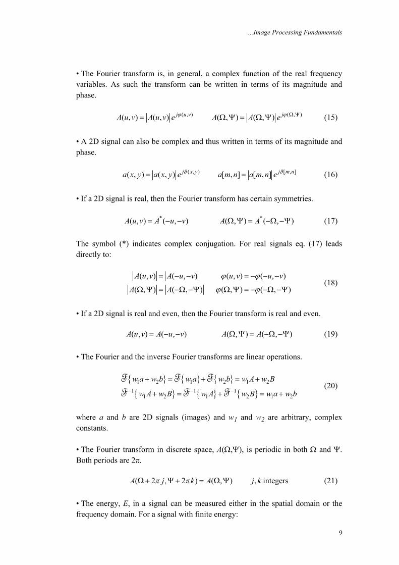
3.4.1 Importance of phase and magnitude Equation (15) indicates that the Fourier transform of an image can be complex. This is illustrated below in Figures 4a-c. Figure 4a shows the original image a[m,n], Figure 4b the magnitude in a scaled form as log(|A(Ω,Ψ)|), and Figure 4c the phase ϕ(Ω,Ψ).
Figure 4a Figure 4b Figure 4c
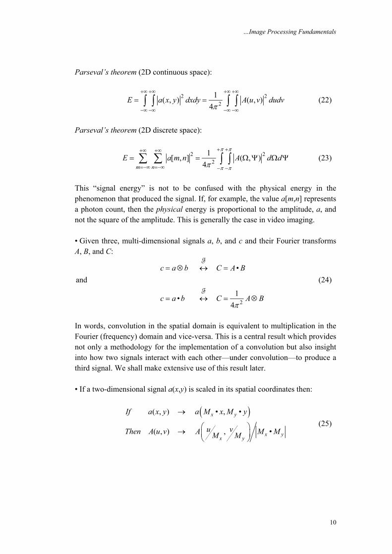
Original log(|A(Ω,Ψ)|) ϕ(Ω,Ψ) Both the magnitude and the phase functions are necessary for the complete reconstruction of an image from its Fourier transform. Figure 5a shows what happens when Figure 4a is restored solely on the basis of the magnitude information and Figure 5b shows what happens when Figure 4a is restored solely on the basis of the phase information.
…Image Processing Fundamentals
12
Figure 5a Figure 5b
ϕ(Ω,Ψ) = 0 |A(Ω,Ψ)| = constant Neither the magnitude information nor the phase information is sufficient to restore the image. The magnitude–only image (Figure 5a) is unrecognizable and has severe dynamic range problems. The phase-only image (Figure 5b) is barely recognizable, that is, severely degraded in quality.
3.4.2 Circularly symmetric signals An arbitrary 2D signal a(x,y) can always be written in a polar coordinate system as a(r,θ). When the 2D signal exhibits a circular symmetry this means that: ( , ) ( , ) ( )a x y a r a rθ= = (28) where r2 = x2 + y2 and tanθ = y/x. As a number of physical systems such as lenses exhibit circular symmetry, it is useful to be able to compute an appropriate Fourier representation. The Fourier transform A(u,v) can be written in polar coordinates A(q,ξ) and then, for a circularly symmetric signal, rewritten as a Hankel transform:
{ } ( )0
( , ) ( , ) 2 ( ) ( )oA u v a x y a r J r q r dr A qπ∞
= = =∫F (29)
where 2 2 2 and tanq u v v uξ= + = and Jo(•) is a Bessel function of the first kind of order zero. The inverse Hankel transform is given by:
( )0
1( ) ( )2 oa r A q J rq q dqπ
∞
= ∫ (30)
…Image Processing Fundamentals
13
The Fourier transform of a circularly symmetric 2D signal is a function of only the radial frequency, q. The dependence on the angular frequency, ξ, has vanished. Further, if a(x,y) = a(r) is real, then it is automatically even due to the circular symmetry. According to equation (19), A(q) will then be real and even.
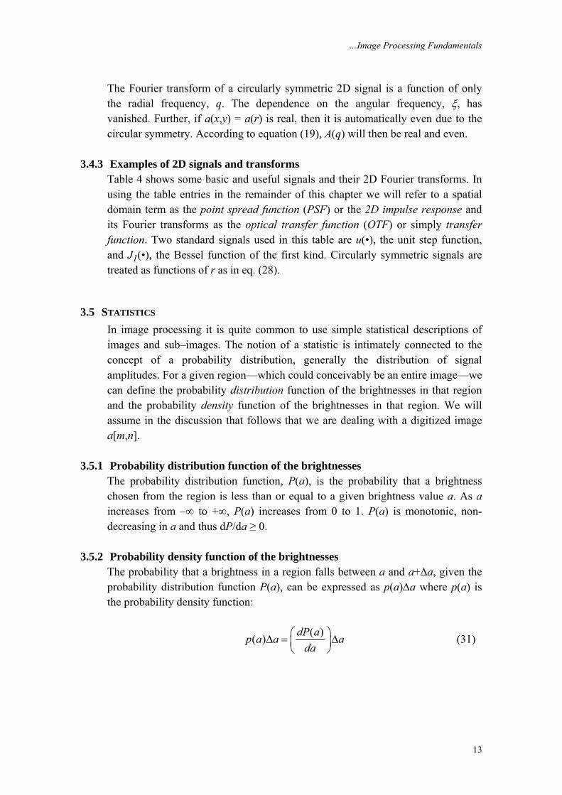
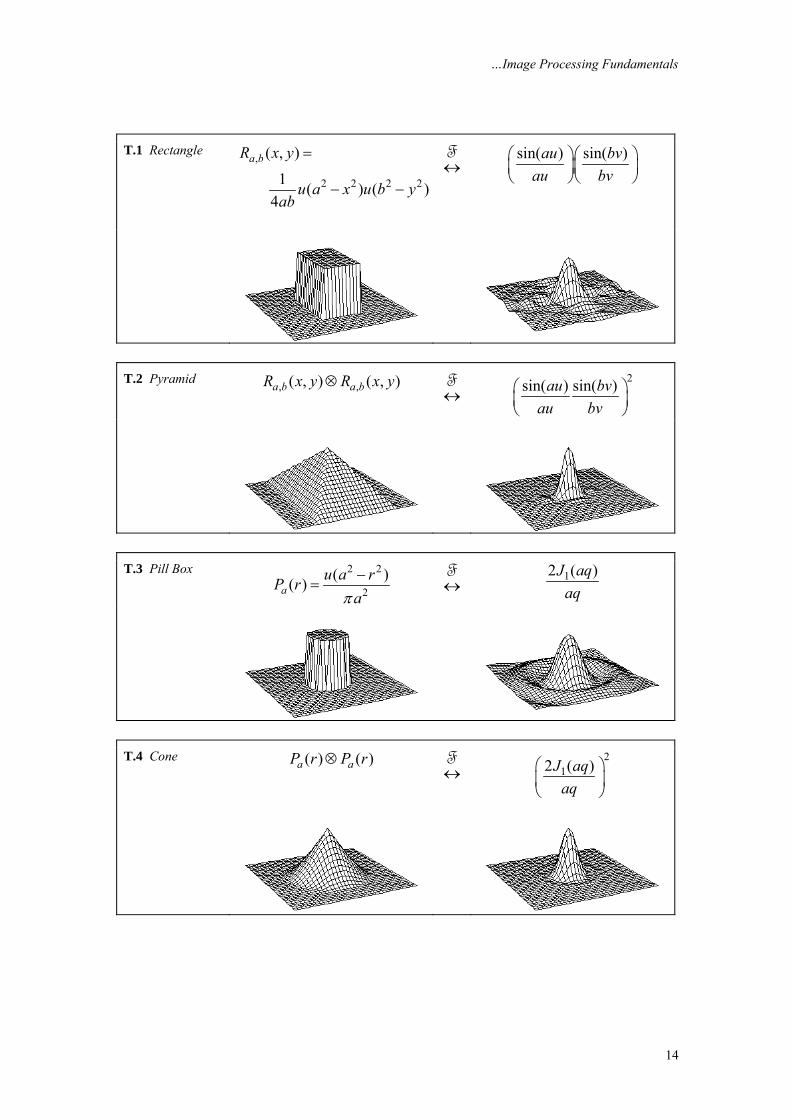
3.4.3 Examples of 2D signals and transforms Table 4 shows some basic and useful signals and their 2D Fourier transforms. In using the table entries in the remainder of this chapter we will refer to a spatial domain term as the point spread function (PSF) or the 2D impulse response and its Fourier transforms as the optical transfer function (OTF) or simply transfer function. Two standard signals used in this table are u(•), the unit step function, and J1(•), the Bessel function of the first kind. Circularly symmetric signals are treated as functions of r as in eq. (28).
3.5 STATISTICS In image processing it is quite common to use simple statistical descriptions of images and sub–images. The notion of a statistic is intimately connected to the concept of a probability distribution, generally the distribution of signal amplitudes. For a given region—which could conceivably be an entire image—we can define the probability distribution function of the brightnesses in that region and the probability density function of the brightnesses in that region. We will assume in the discussion that follows that we are dealing with a digitized image a[m,n].
3.5.1 Probability distribution function of the brightnesses The probability distribution function, P(a), is the probability that a brightness chosen from the region is less than or equal to a given brightness value a. As a increases from –∞ to +∞, P(a) increases from 0 to 1. P(a) is monotonic, non-decreasing in a and thus dP/da ≥ 0.
3.5.2 Probability density function of the brightnesses The probability that a brightness in a region falls between a and a+Δa, given the probability distribution function P(a), can be expressed as p(a)Δa where p(a) is the probability density function:
( )( ) dP ap a a ada
⎛ ⎞Δ = Δ⎜ ⎟⎝ ⎠
(31)
…Image Processing Fundamentals
14
T.1 Rectangle
,
2 2 2 2
( , )
1 ( ) ( )4
a bR x y
u a x u b yab
=
− −
↔F
sin( ) sin( )au bv
au bv⎛ ⎞⎛ ⎞⎜ ⎟⎜ ⎟⎝ ⎠⎝ ⎠
T.2 Pyramid
, ,( , ) ( , )a b a bR x y R x y⊗ ↔F
2sin( ) sin( )au bv
au bv⎛ ⎞⎜ ⎟⎝ ⎠
T.3 Pill Box 2 2
2( )( )a
u a rP raπ−
= ↔F
12 ( )J aqaq
T.4 Cone ( ) ( )a aP r P r⊗
↔F
2
12 ( )J aqaq
⎛ ⎞⎜ ⎟⎝ ⎠
…Image Processing Fundamentals
15
T.5 Airy PSF 21
1 2( )1( ) cJ q rPSF r
rπ⎛ ⎞
= ⎜ ⎟⎝ ⎠
↔F
( )2
1 2 22 cos 1
with 2
cc c c
c
q q q u q qq q q
q NA
π
π λ
−⎛ ⎞⎛ ⎞⎜ ⎟− − −⎜ ⎟⎜ ⎟⎜ ⎟⎝ ⎠⎝ ⎠
=
T.6 Gaussian
( )2
2 2 21, exp
2 2Drg r σ
πσ σ
⎛ ⎞= −⎜ ⎟⎜ ⎟
⎝ ⎠↔F
( ) ( )2 2
2 , exp 2DG q qσ σ= −
T.7 Peak 1
r ↔
F
2qπ
T.8 Exponential
Decay are−
↔F
( )3/ 22 2
2 a
q a
π
+
Table 4: 2D Images and their Fourier Transforms
…Image Processing Fundamentals
16
Because of the monotonic, non-decreasing character of P(a) we have that:
–
( ) 0 and ( ) 1p a p a da+∞
∞
≥ =∫ (32)
For an image with quantized (integer) brightness amplitudes, the interpretation of Δa is the width of a brightness interval. We assume constant width intervals. The brightness probability density function is frequently estimated by counting the number of times that each brightness occurs in the region to generate a histogram, h[a]. The histogram can then be normalized so that the total area under the histogram is 1 (eq. (32)). Said another way, the p[a] for a region is the normalized count of the number of pixels, Λ, in a region that have quantized brightness a:
1[ ] [ ] with [ ]a
p a h a h a= Λ =Λ ∑ (33)
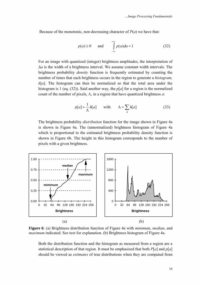
The brightness probability distribution function for the image shown in Figure 4a is shown in Figure 6a. The (unnormalized) brightness histogram of Figure 4a which is proportional to the estimated brightness probability density function is shown in Figure 6b. The height in this histogram corresponds to the number of pixels with a given brightness.
0.00
0.25
0.50
0.75
1.00
0 32 64 96 128 160 192 224 256
Brightness
mimimum
median
maximum
0
400
800
1200
1600
0 32 64 96 128 160 192 224 256
Brightness
(a) (b)
Figure 6: (a) Brightness distribution function of Figure 4a with minimum, median, and maximum indicated. See text for explanation. (b) Brightness histogram of Figure 4a.
Both the distribution function and the histogram as measured from a region are a statistical description of that region. It must be emphasized that both P[a] and p[a] should be viewed as estimates of true distributions when they are computed from
…Image Processing Fundamentals
17
a specific region. That is, we view an image and a specific region as one realization of the various random processes involved in the formation of that image and that region. In the same context, the statistics defined below must be viewed as estimates of the underlying parameters.
3.5.3 Average The average brightness of a region is defined as the sample mean of the pixel brightnesses within that region. The average, ma, of the brightnesses over the Λ pixels within a region (ℜ) is given by:
( , )
1 [ , ]am n
m a m n∈ℜ
=Λ ∑ (34)
Alternatively, we can use a formulation based upon the (unnormalized) brightness histogram, h(a) = Λ•p(a), with discrete brightness values a. This gives:
1 • [ ]aa
m a h a=Λ ∑ (35)
The average brightness, ma, is an estimate of the mean brightness, μa, of the underlying brightness probability distribution.
3.5.4 Standard deviation The unbiased estimate of the standard deviation, sa, of the brightnesses within a region (ℜ) with Λ pixels is called the sample standard deviation and is given by:
( )2
,
2 2
,
1 [ , ]1
[ , ]
1
a am n
am n
s a m n m
a m n m
∈ℜ
∈ℜ
= −Λ −
− Λ
=Λ −
∑
∑ (36)
Using the histogram formulation gives:
2 2• [ ] •
1
aa
a
a h a ms
⎛ ⎞− Λ⎜ ⎟
⎝ ⎠=Λ −
∑ (37)
The standard deviation, sa, is an estimate of σa of the underlying brightness probability distribution.
…Image Processing Fundamentals
18
3.5.5 Coefficient-of-variation The dimensionless coefficient–of–variation, CV, is defined as:
100%a
a
sCVm
= × (38)
3.5.6 Percentiles The percentile, p%, of an unquantized brightness distribution is defined as that value of the brightness a such that:
P(a) = p% or equivalently
–
( ) %a
p d pα α∞
=∫ (39)
Three special cases are frequently used in digital image processing. • 0% the minimum value in the region • 50% the median value in the region • 100% the maximum value in the region All three of these values can be determined from Figure 6a.
3.5.7 Mode The mode of the distribution is the most frequent brightness value. There is no guarantee that a mode exists or that it is unique.
3.5.8 Signal–to–Noise ratio The signal–to–noise ratio, SNR, can have several definitions. The noise is characterized by its standard deviation, sn. The characterization of the signal can differ. If the signal is known to lie between two boundaries, amin ≤ a ≤ amax, then the SNR is defined as:
Bounded signal – max min1020log
n
a aSNR dBs
⎛ ⎞−= ⎜ ⎟
⎝ ⎠ (40)
If the signal is not bounded but has a statistical distribution then two other definitions are known: Stochastic signal –
S & N inter-dependent 1020 log a
n
mSNR dBs
⎛ ⎞= ⎜ ⎟
⎝ ⎠ (41)
…Image Processing Fundamentals
19
S & N independent 1020 log a
n
sSNR dBs
⎛ ⎞= ⎜ ⎟
⎝ ⎠ (42)
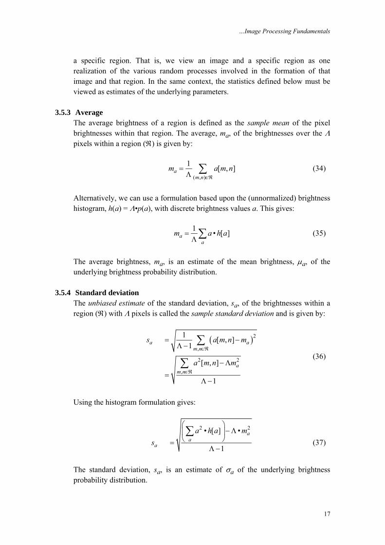
where ma and sa are defined above. The various statistics are given in Table 5 for the image and the region shown in Figure 7.
Statistic Image ROIAverage 137.7 219.3Standard Deviation 49.5 4.0Minimum 56 202Median 141 220Maximum 241 226Mode 62 220SNR (db) NA 33.3
Figure 7 Table 5 Region is the interior of the circle. Statistics from Figure 7
A SNR calculation for the entire image based on eq. (40) is not directly available. The variations in the image brightnesses that lead to the large value of s (=49.5) are not, in general, due to noise but to the variation in local information. With the help of the region there is a way to estimate the SNR. We can use the sℜ (=4.0) and the dynamic range, amax – amin, for the image (=241–56) to calculate a global SNR (=33.3 dB). The underlying assumptions are that 1) the signal is approximately constant in that region and the variation in the region is therefore due to noise, and, 2) that the noise is the same over the entire image with a standard deviation given by sn = sℜ.
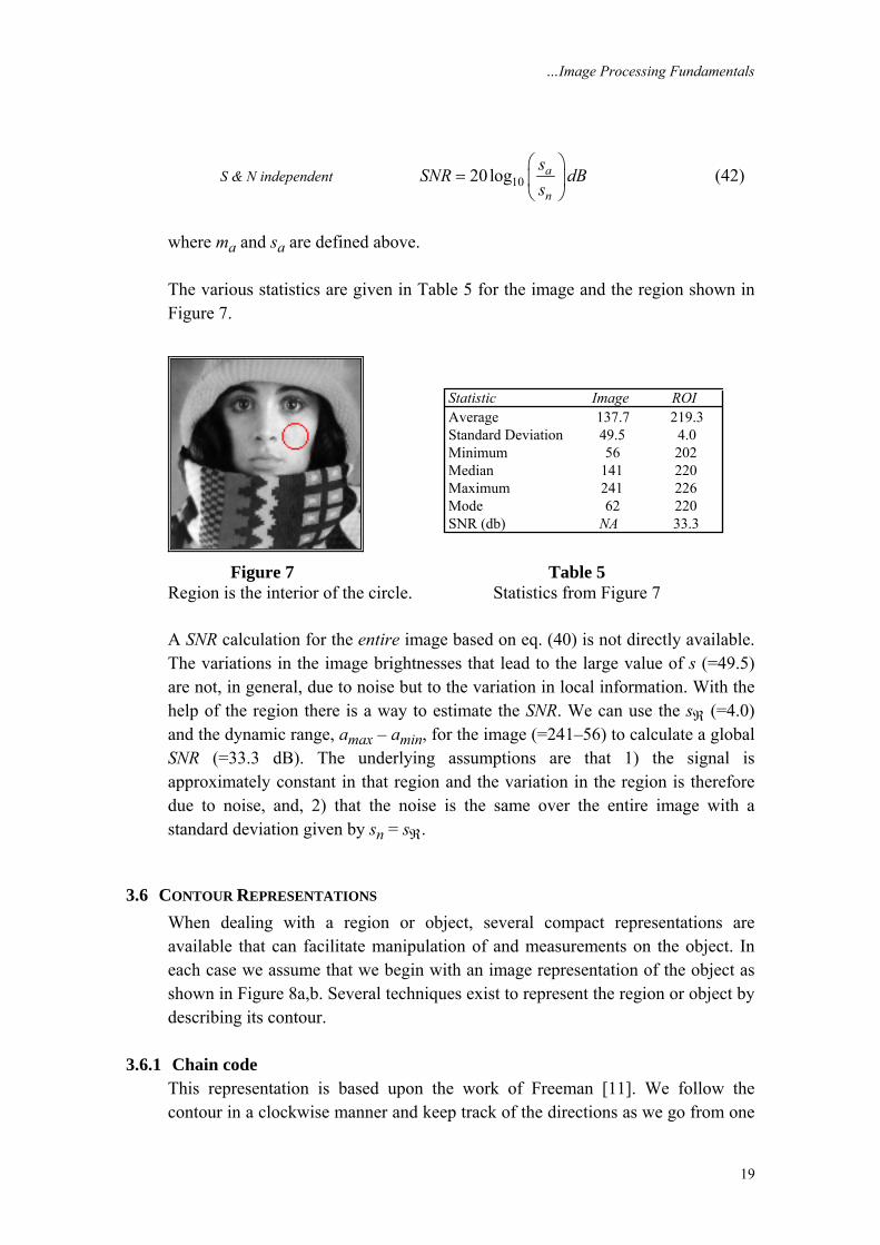
3.6 CONTOUR REPRESENTATIONS When dealing with a region or object, several compact representations are available that can facilitate manipulation of and measurements on the object. In each case we assume that we begin with an image representation of the object as shown in Figure 8a,b. Several techniques exist to represent the region or object by describing its contour.
3.6.1 Chain code This representation is based upon the work of Freeman [11]. We follow the contour in a clockwise manner and keep track of the directions as we go from one
…Image Processing Fundamentals
20
contour pixel to the next. For the standard implementation of the chain code we consider a contour pixel to be an object pixel that has a background (non-object) pixel as one or more of its 4-connected neighbors. See Figures 3a and 8c. The codes associated with eight possible directions are the chain codes and, with x as the current contour pixel position, the codes are generally defined as:
3 2 14 05 6 7
Chain codes x= (43)
Digitization
Run LengthsContour(a) (b)
(c) (d)
Figure 8: Region (shaded) as it is transformed from (a) continuous to (b) discrete form and then considered as a (c) contour or (d) run lengths illustrated in alternating colors.
3.6.2 Chain code properties • Even codes {0,2,4,6} correspond to horizontal and vertical directions; odd codes {1,3,5,7} correspond to the diagonal directions. • Each code can be considered as the angular direction, in multiples of 45°, that we must move to go from one contour pixel to the next. • The absolute coordinates [m,n] of the first contour pixel (e.g. top, leftmost) together with the chain code of the contour represent a complete description of the discrete region contour.
…Image Processing Fundamentals
21
• When there is a change between two consecutive chain codes, then the contour has changed direction. This point is defined as a corner.
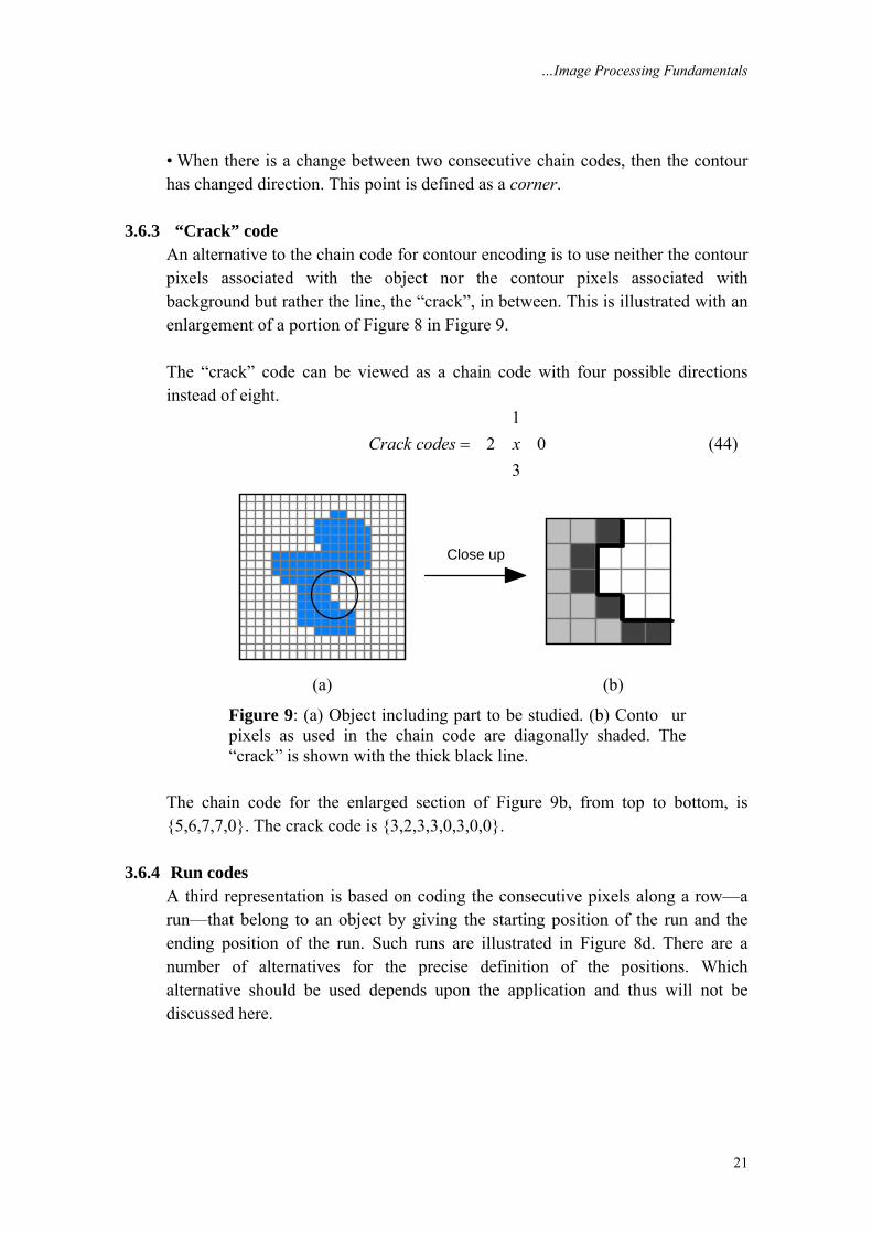
3.6.3 “Crack” code An alternative to the chain code for contour encoding is to use neither the contour pixels associated with the object nor the contour pixels associated with background but rather the line, the “crack”, in between. This is illustrated with an enlargement of a portion of Figure 8 in Figure 9. The “crack” code can be viewed as a chain code with four possible directions instead of eight.
1
2 03
Crack codes x= (44)
Close up
(a) (b)
Figure 9: (a) Object including part to be studied. (b) Conto ur pixels as used in the chain code are diagonally shaded. The “crack” is shown with the thick black line.
The chain code for the enlarged section of Figure 9b, from top to bottom, is {5,6,7,7,0}. The crack code is {3,2,3,3,0,3,0,0}.
3.6.4 Run codes A third representation is based on coding the consecutive pixels along a row—a run—that belong to an object by giving the starting position of the run and the ending position of the run. Such runs are illustrated in Figure 8d. There are a number of alternatives for the precise definition of the positions. Which alternative should be used depends upon the application and thus will not be discussed here.
…Image Processing Fundamentals
22
4. Perception Many image processing applications are intended to produce images that are to be viewed by human observers (as opposed to, say, automated industrial inspection.) It is therefore important to understand the characteristics and limitations of the human visual system—to understand the “receiver” of the 2D signals. At the outset it is important to realize that 1) the human visual system is not well understood, 2) no objective measure exists for judging the quality of an image that corresponds to human assessment of image quality, and, 3) the “typical” human observer does not exist. Nevertheless, research in perceptual psychology has provided some important insights into the visual system. See, for example, Stockham [12].
4.1 BRIGHTNESS SENSITIVITY There are several ways to describe the sensitivity of the human visual system. To begin, let us assume that a homogeneous region in an image has an intensity as a function of wavelength (color) given by I(λ). Further let us assume that I(λ) = Io, a constant.
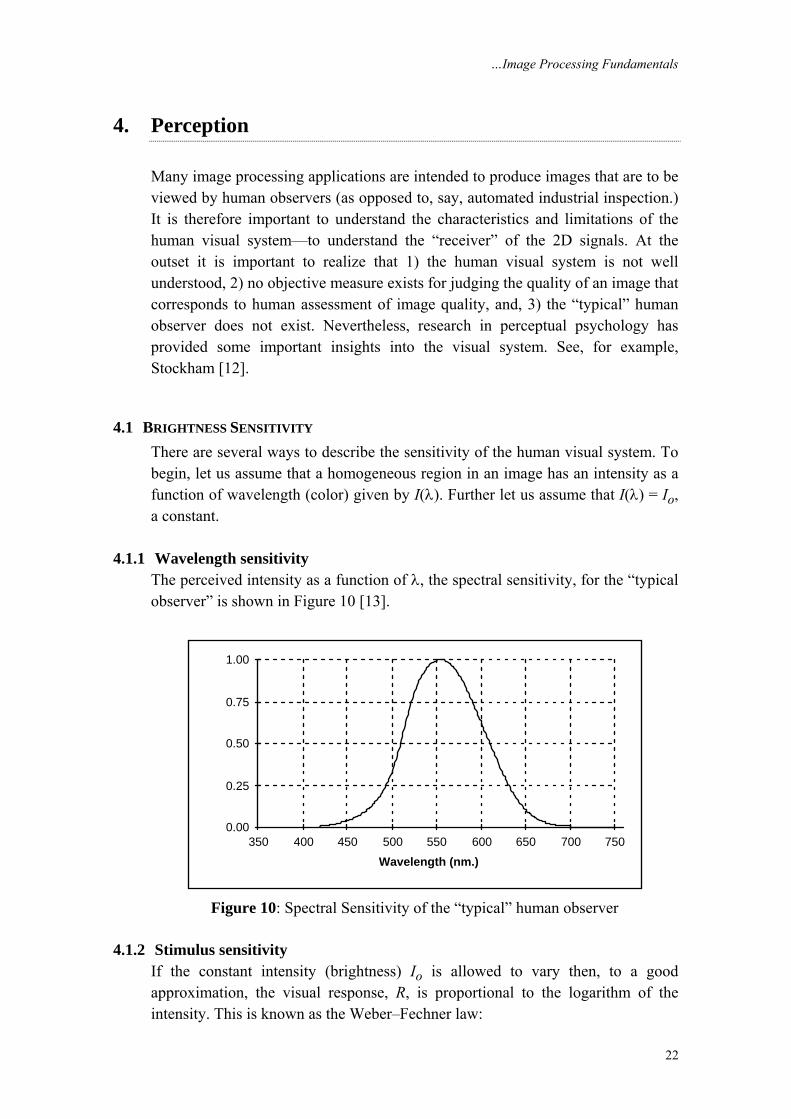
4.1.1 Wavelength sensitivity The perceived intensity as a function of λ, the spectral sensitivity, for the “typical observer” is shown in Figure 10 [13].
0.00
0.25
0.50
0.75
1.00
350 400 450 500 550 600 650 700 750
Wavelength (nm.)
Figure 10: Spectral Sensitivity of the “typical” human observer
4.1.2 Stimulus sensitivity If the constant intensity (brightness) Io is allowed to vary then, to a good approximation, the visual response, R, is proportional to the logarithm of the intensity. This is known as the Weber–Fechner law:
…Image Processing Fundamentals
23
( )log oR I= (45)
The implications of this are easy to illustrate. Equal perceived steps in brightness, ΔR = k, require that the physical brightness (the stimulus) increases exponentially. This is illustrated in Figure 11ab. A horizontal line through the top portion of Figure 11a shows a linear increase in objective brightness (Figure 11b) but a logarithmic increase in subjective brightness. A horizontal line through the bottom portion of Figure 11a shows an exponential increase in objective brightness (Figure 11b) but a linear increase in subjective brightness.
0
64
128
192
25616 48 80 112
144
176
208
240
Sampled Postion
ΔI=k
ΔI=k•I
Figure 11a Figure 11b
(top) Brightness step ΔI = k Actual brightnesses plus interpolated values
(bottom) Brightness step ΔI = k•I The Mach band effect is visible in Figure 11a. Although the physical brightness is constant across each vertical stripe, the human observer perceives an “undershoot” and “overshoot” in brightness at what is physically a step edge. Thus, just before the step, we see a slight decrease in brightness compared to the true physical value. After the step we see a slight overshoot in brightness compared to the true physical value. The total effect is one of increased, local, perceived contrast at a step edge in brightness.
4.2 SPATIAL FREQUENCY SENSITIVITY If the constant intensity (brightness) Io is replaced by a sinusoidal grating with increasing spatial frequency (Figure 12a), it is possible to determine the spatial frequency sensitivity. The result is shown in Figure 12b [14, 15].
…Image Processing Fundamentals
24
1
10
100
1000
1 10 100Spatial Frequency
(cycles/degree)
Figure 12a Figure 12b
Sinusoidal test grating Spatial frequency sensitivity To translate these data into common terms, consider an “ideal” computer monitor at a viewing distance of 50 cm. The spatial frequency that will give maximum response is at 10 cycles per degree. (See Figure 12b.) The one degree at 50 cm translates to 50 tan(1°) = 0.87 cm on the computer screen. Thus the spatial frequency of maximum response fmax = 10 cycles/0.87 cm = 11.46 cycles/cm at this viewing distance. Translating this into a general formula gives:
max10 572.9 /
• tan(1 )f cycles cm
d d= =
° (46)
where d = viewing distance measured in cm.
4.3 COLOR SENSITIVITY Human color perception is an exceedingly complex topic. As such we can only present a brief introduction here. The physical perception of color is based upon three color pigments in the retina.
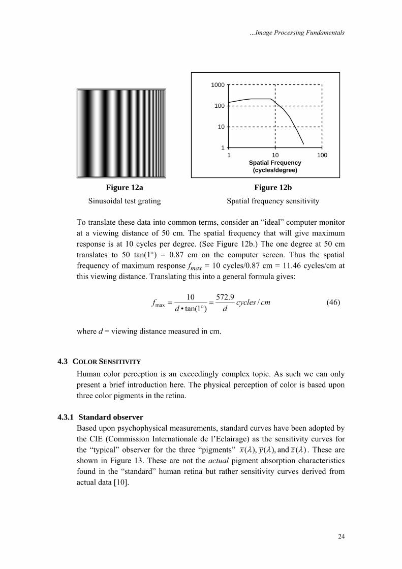
4.3.1 Standard observer Based upon psychophysical measurements, standard curves have been adopted by the CIE (Commission Internationale de l’Eclairage) as the sensitivity curves for the “typical” observer for the three “pigments” ( ), ( ), and ( )x y zλ λ λ . These are shown in Figure 13. These are not the actual pigment absorption characteristics found in the “standard” human retina but rather sensitivity curves derived from actual data [10].
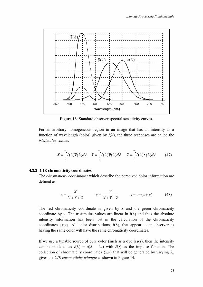
…Image Processing Fundamentals
25
350 400 450 500 550 600 650 700 750
Wavelength (nm.)
x (λ )y (λ )
z (λ )
Figure 13: Standard observer spectral sensitivity curves.
For an arbitrary homogeneous region in an image that has an intensity as a function of wavelength (color) given by I(λ), the three responses are called the tristimulus values:
0 0 0
( ) ( ) ( ) ( ) ( ) ( )X I x d Y I y d Z I z dλ λ λ λ λ λ λ λ λ∞ ∞ ∞
= = =∫ ∫ ∫ (47)
4.3.2 CIE chromaticity coordinates The chromaticity coordinates which describe the perceived color information are defined as:
1 ( )X Yx y z x yX Y Z X Y Z
= = = − ++ + + +
(48)
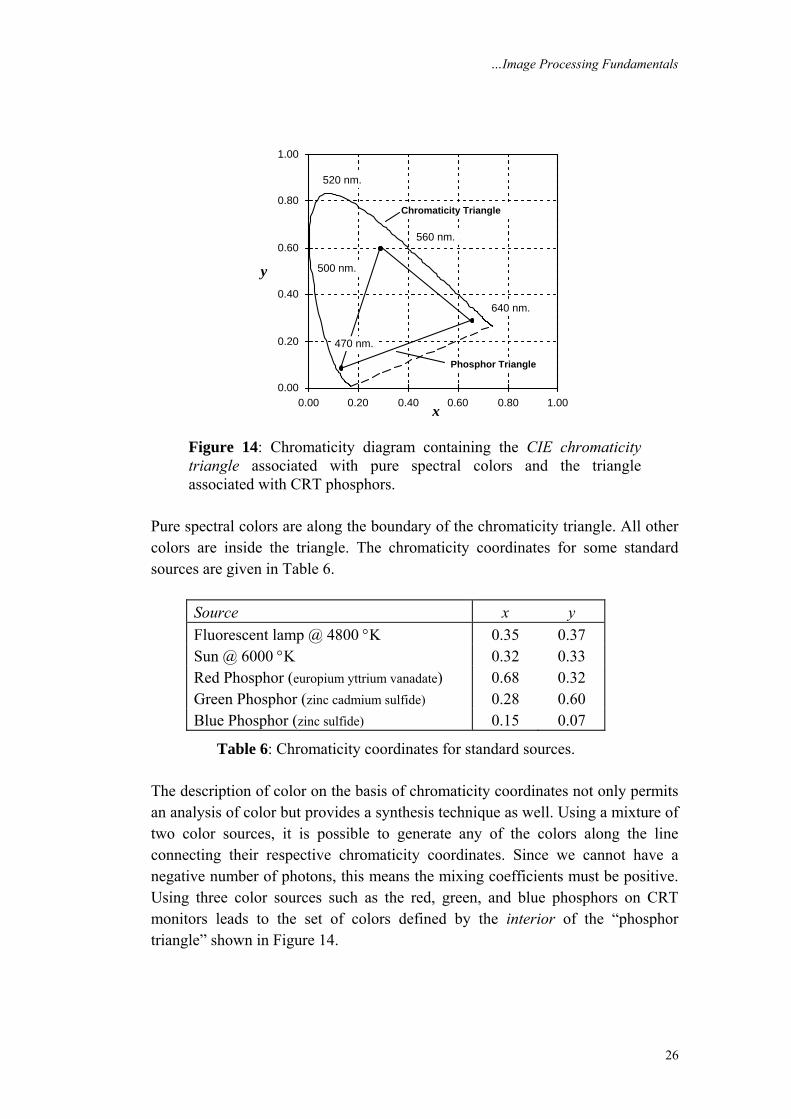
The red chromaticity coordinate is given by x and the green chromaticity coordinate by y. The tristimulus values are linear in I(λ) and thus the absolute intensity information has been lost in the calculation of the chromaticity coordinates {x,y}. All color distributions, I(λ), that appear to an observer as having the same color will have the same chromaticity coordinates. If we use a tunable source of pure color (such as a dye laser), then the intensity can be modeled as I(λ) = δ(λ – λo) with δ(•) as the impulse function. The collection of chromaticity coordinates {x,y} that will be generated by varying λo gives the CIE chromaticity triangle as shown in Figure 14.
…Image Processing Fundamentals
26
0.00
0.20
0.40
0.60
0.80
1.00
0.00 0.20 0.40 0.60 0.80 1.00x
y
520 nm.
560 nm.
640 nm.
500 nm.
Chromaticity Triangle
Phosphor Triangle
470 nm.
Figure 14: Chromaticity diagram containing the CIE chromaticity triangle associated with pure spectral colors and the triangle associated with CRT phosphors.
Pure spectral colors are along the boundary of the chromaticity triangle. All other colors are inside the triangle. The chromaticity coordinates for some standard sources are given in Table 6.
Source x y Fluorescent lamp @ 4800 °K 0.35 0.37 Sun @ 6000 °K 0.32 0.33 Red Phosphor (europium yttrium vanadate) 0.68 0.32 Green Phosphor (zinc cadmium sulfide) 0.28 0.60 Blue Phosphor (zinc sulfide) 0.15 0.07
Table 6: Chromaticity coordinates for standard sources. The description of color on the basis of chromaticity coordinates not only permits an analysis of color but provides a synthesis technique as well. Using a mixture of two color sources, it is possible to generate any of the colors along the line connecting their respective chromaticity coordinates. Since we cannot have a negative number of photons, this means the mixing coefficients must be positive. Using three color sources such as the red, green, and blue phosphors on CRT monitors leads to the set of colors defined by the interior of the “phosphor triangle” shown in Figure 14.
…Image Processing Fundamentals
27
The formulas for converting from the tristimulus values (X,Y,Z) to the well-known CRT colors (R,G,B) and back are given by:
1.9107 0.5326 0.28830.9843 1.9984 0.0283 •
0.0583 0.1185 0.8986
R XG YB Z
− −⎡ ⎤ ⎡ ⎤ ⎡ ⎤⎢ ⎥ ⎢ ⎥ ⎢ ⎥= − −⎢ ⎥ ⎢ ⎥ ⎢ ⎥⎢ ⎥ ⎢ ⎥ ⎢ ⎥−⎣ ⎦ ⎣ ⎦ ⎣ ⎦
(49)
and
0.6067 0.1736 0.20010.2988 0.5868 0.1143 •0.0000 0.0661 1.1149
X RY GZ B
⎡ ⎤ ⎡ ⎤ ⎡ ⎤⎢ ⎥ ⎢ ⎥ ⎢ ⎥=⎢ ⎥ ⎢ ⎥ ⎢ ⎥⎢ ⎥ ⎢ ⎥ ⎢ ⎥⎣ ⎦ ⎣ ⎦ ⎣ ⎦
(50)
As long as the position of a desired color (X,Y,Z) is inside the phosphor triangle in Figure 14, the values of R, G, and B as computed by eq. (49) will be positive and can therefore be used to drive a CRT monitor. It is incorrect to assume that a small displacement anywhere in the chromaticity diagram (Figure 14) will produce a proportionally small change in the perceived color. An empirically-derived chromaticity space where this property is approximated is the (u’,v’) space:
4 9' '2 12 3 2 12 3
and9 ' 4 '
6 ' 16 ' 12 6 ' 16 ' 12
x yu vx y x y
u vx yu v u v
= =− + + − + +
= =− + − +
(51)
Small changes almost anywhere in the (u’,v’) chromaticity space produce equally small changes in the perceived colors.
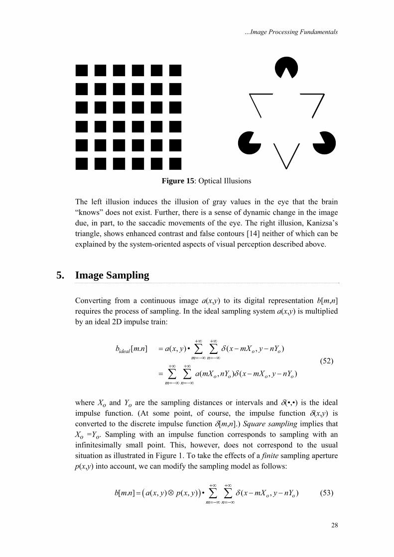
4.4 OPTICAL ILLUSIONS The description of the human visual system presented above is couched in standard engineering terms. This could lead one to conclude that there is sufficient knowledge of the human visual system to permit modeling the visual system with standard system analysis techniques. Two simple examples of optical illusions, shown in Figure 15, illustrate that this system approach would be a gross oversimplification. Such models should only be used with extreme care.
…Image Processing Fundamentals
28
Figure 15: Optical Illusions
The left illusion induces the illusion of gray values in the eye that the brain “knows” does not exist. Further, there is a sense of dynamic change in the image due, in part, to the saccadic movements of the eye. The right illusion, Kanizsa’s triangle, shows enhanced contrast and false contours [14] neither of which can be explained by the system-oriented aspects of visual perception described above.
5. Image Sampling Converting from a continuous image a(x,y) to its digital representation b[m,n] requires the process of sampling. In the ideal sampling system a(x,y) is multiplied by an ideal 2D impulse train:
[ . ] ( , ) • ( , )
( , ) ( , )
ideal o om n
o o o om n
b m n a x y x mX y nY
a mX nY x mX y nY
δ
δ
+∞ +∞
=−∞ =−∞+∞ +∞
=−∞ =−∞
= − −
= − −
∑ ∑
∑ ∑ (52)
where Xo and Yo are the sampling distances or intervals and δ(•,•) is the ideal impulse function. (At some point, of course, the impulse function δ(x,y) is converted to the discrete impulse function δ[m,n].) Square sampling implies that Xo =Yo. Sampling with an impulse function corresponds to sampling with an infinitesimally small point. This, however, does not correspond to the usual situation as illustrated in Figure 1. To take the effects of a finite sampling aperture p(x,y) into account, we can modify the sampling model as follows:
( )[ . ] ( , ) ( , ) • ( , )o om n
b m n a x y p x y x mX y nYδ+∞ +∞
=−∞ =−∞
= ⊗ − −∑ ∑ (53)
…Image Processing Fundamentals
29
The combined effect of the aperture and sampling are best understood by examining the Fourier domain representation.
21( , ) ( , ) • ( , )
4 s s s sm n
B A m n P m nπ
+∞ +∞
=−∞ =−∞
Ω Ψ = Ω − Ω Ψ − Ψ Ω − Ω Ψ − Ψ∑ ∑ (54)
where Ωs = 2π/Xo is the sampling frequency in the x direction and Ψs = 2π/Yo is the sampling frequency in the y direction. The aperture p(x,y) is frequently square, circular, or Gaussian with the associated P(Ω,Ψ). (See Table 4.) The periodic nature of the spectrum, described in eq. (21) is clear from eq. (54).
5.1 SAMPLING DENSITY FOR IMAGE PROCESSING To prevent the possible aliasing (overlapping) of spectral terms that is inherent in eq. (54) two conditions must hold: • Bandlimited A(u,v) – ( , ) 0 for andc cA u v u u v v≡ > > (55)
• Nyquist sampling frequency – 2 • and 2•s c s cu vΩ > Ψ > (56) where uc and vc are the cutoff frequencies in the x and y direction, respectively. Images that are acquired through lenses that are circularly-symmetric, aberration-free, and diffraction-limited will, in general, be bandlimited. The lens acts as a lowpass filter with a cutoff frequency in the frequency domain (eq. (11)) given by:
2c c
NAu vλ
= = (57)
where NA is the numerical aperture of the lens and λ is the shortest wavelength of light used with the lens [16]. If the lens does not meet one or more of these assumptions then it will still be bandlimited but at lower cutoff frequencies than those given in eq. (57). When working with the F-number (F) of the optics instead of the NA and in air (with index of refraction = 1.0), eq. (57) becomes:
2
2 1
4 1c cu v
Fλ⎛ ⎞
= = ⎜ ⎟⎜ ⎟+⎝ ⎠ (58)
…Image Processing Fundamentals
30
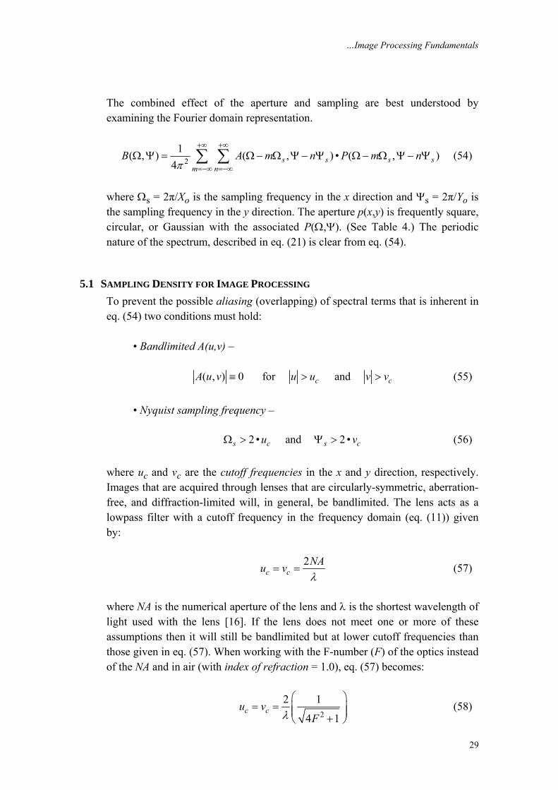
5.1.1 Sampling aperture The aperture p(x,y) described above will have only a marginal effect on the final signal if the two conditions eqs. (56) and (57) are satisfied. Given, for example, the distance between samples Xo equals Yo and a sampling aperture that is not wider than Xo, the effect on the overall spectrum—due to the A(u,v)P(u,v) behavior implied by eq.(53)—is illustrated in Figure 16 for square and Gaussian apertures. The spectra are evaluated along one axis of the 2D Fourier transform. The Gaussian aperture in Figure 16 has a width such that the sampling interval Xo contains ±3σ (99.7%) of the Gaussian. The rectangular apertures have a width such that one occupies 95% of the sampling interval and the other occupies 50% of the sampling interval. The 95% width translates to a fill factor of 90% and the 50% width to a fill factor of 25%. The fill factor is discussed in Section 7.5.2.
0.6
0.7
0.8
0.9
1.0
0.0 0.1 0.2 0.3 0.4 0.5Fraction of Nyquist frequency
— Square aperture, fill = 25%
— Square aperture, fill = 90%
— Gaussian aperture
Figure 16: Aperture spectra P(u,v=0) for frequencies up to half the Nyquist frequency. For explanation of “fill” see text.
5.2 SAMPLING DENSITY FOR IMAGE ANALYSIS The “rules” for choosing the sampling density when the goal is image analysis—as opposed to image processing—are different. The fundamental difference is that the digitization of objects in an image into a collection of pixels introduces a form of spatial quantization noise that is not bandlimited. This leads to the following results for the choice of sampling density when one is interested in the measurement of area and (perimeter) length.
…Image Processing Fundamentals
31
5.2.1 Sampling for area measurements Assuming square sampling, Xo = Yo and the unbiased algorithm for estimating area which involves simple pixel counting, the CV (see eq. (38)) of the area measurement is related to the sampling density by [17]: 3 2 2
2 32 : lim ( ) 3 : lim ( )S S
D CV S k S D CV S k S− −
→∞ →∞= = (59)
and in D dimensions: ( 1) 2lim ( ) D
DSCV S k S − +
→∞= (60)
where S is the number of samples per object diameter. In 2D the measurement is area, in 3D volume, and in D-dimensions hypervolume.
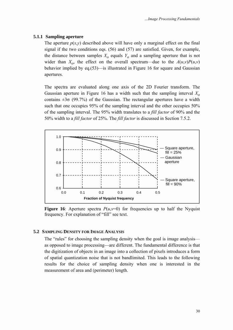
5.2.2 Sampling for length measurements Again assuming square sampling and algorithms for estimating length based upon the Freeman chain-code representation (see Section 3.6.1), the CV of the length measurement is related to the sampling density per unit length as shown in Figure 17 (see [18, 19].)
0.1%
1.0%
10.0%
100.0%
1 10 100 1000
Sampling Density / Unit Length
Pixel CountFreeman
Kulpa
Corner Count
Figure 17: CV of length measurement for various algorithms.
The curves in Figure 17 were developed in the context of straight lines but similar results have been found for curves and closed contours. The specific formulas for length estimation use a chain code representation of a line and are based upon a linear combination of three numbers: • • •e o cL N N Nα β γ= + + (61)
…Image Processing Fundamentals
32
where Ne is the number of even chain codes, No the number of odd chain codes, and Nc the number of corners. The specific formulas are given in Table 7. Coefficients α β γ
Formula Reference
Pixel count 1 1 0 [18] Freeman 1 2 0 [11] Kulpa 0.9481 0.9481 • 2 0 [20] Corner count 0.980 1.406 –0.091 [21]
Table 7: Length estimation formulas based on chain code counts (Ne, No, Nc)
5.2.3 Conclusions on sampling If one is interested in image processing, one should choose a sampling density based upon classical signal theory, that is, the Nyquist sampling theory. If one is interested in image analysis, one should choose a sampling density based upon the desired measurement accuracy (bias) and precision (CV). In a case of uncertainty, one should choose the higher of the two sampling densities (frequencies).
6. Noise Images acquired through modern sensors may be contaminated by a variety of noise sources. By noise we refer to stochastic variations as opposed to deterministic distortions such as shading or lack of focus. We will assume for this section that we are dealing with images formed from light using modern electro-optics. In particular we will assume the use of modern, charge-coupled device (CCD) cameras where photons produce electrons that are commonly referred to as photoelectrons. Nevertheless, most of the observations we shall make about noise and its various sources hold equally well for other imaging modalities. While modern technology has made it possible to reduce the noise levels associated with various electro-optical devices to almost negligible levels, one noise source can never be eliminated and thus forms the limiting case when all other noise sources are “eliminated”.
6.1 PHOTON NOISE When the physical signal that we observe is based upon light, then the quantum nature of light plays a significant role. A single photon at λ = 500 nm carries an energy of E = hν = hc/λ = 3.97 × 10⁻¹⁹ Joules. Modern CCD cameras are sensitive enough to be able to count individual photons. (Camera sensitivity will be discussed in Section 7.2.) The noise problem arises from the fundamentally
…Image Processing Fundamentals
33
statistical nature of photon production. We cannot assume that, in a given pixel for two consecutive but independent observation intervals of length T, the same number of photons will be counted. Photon production is governed by the laws of quantum physics which restrict us to talking about an average number of photons within a given observation window. The probability distribution for p photons in an observation window of length T seconds is known to be Poisson:
( )( | , )!
p TT eP p T
p
ρρρ
−
= (62)
where ρ is the rate or intensity parameter measured in photons per second. It is critical to understand that even if there were no other noise sources in the imaging chain, the statistical fluctuations associated with photon counting over a finite time interval T would still lead to a finite signal-to-noise ratio (SNR). If we use the appropriate formula for the SNR (eq. (41)), then due to the fact that the average value and the standard deviation are given by:
Poisson process – average T
T
ρ
σ ρ
=
= (63)
we have for the SNR: Photon noise – 1010log ( ) SNR T dBρ= (64) The three traditional assumptions about the relationship between signal and noise do not hold for photon noise: • photon noise is not independent of the signal; • photon noise is not Gaussian, and; • photon noise is not additive. For very bright signals, where ρT exceeds 105, the noise fluctuations due to photon statistics can be ignored if the sensor has a sufficiently high saturation level. This will be discussed further in Section 7.3 and, in particular, eq. (73).
6.2 THERMAL NOISE An additional, stochastic source of electrons in a CCD well is thermal energy. Electrons can be freed from the CCD material itself through thermal vibration and then, trapped in the CCD well, be indistinguishable from “true” photoelectrons. By cooling the CCD chip it is possible to reduce significantly the number of “thermal electrons” that give rise to thermal noise or dark current. As the
…Image Processing Fundamentals
34
integration time T increases, the number of thermal electrons increases. The probability distribution of thermal electrons is also a Poisson process where the rate parameter is an increasing function of temperature. There are alternative techniques (to cooling) for suppressing dark current and these usually involve estimating the average dark current for the given integration time and then subtracting this value from the CCD pixel values before the A/D converter. While this does reduce the dark current average, it does not reduce the dark current standard deviation and it also reduces the possible dynamic range of the signal.
6.3 ON-CHIP ELECTRONIC NOISE This noise originates in the process of reading the signal from the sensor, in this case through the field effect transistor (FET) of a CCD chip. The general form of the power spectral density of readout noise is:
Readout noise – min
min max
max
0( )
0nnS k
β
α
ω ω ω βω ω ω ω
ω ω αω
−⎧ < >⎪
∝ < <⎨⎪ > >⎩
(65)
where α and β are constants and ω is the (radial) frequency at which the signal is transferred from the CCD chip to the “outside world.” At very low readout rates (ω < ωmin) the noise has a 1/ƒ character. Readout noise can be reduced to manageable levels by appropriate readout rates and proper electronics. At very low signal levels (see eq. (64)), however, readout noise can still become a significant component in the overall SNR [22].
6.4 KTC NOISE Noise associated with the gate capacitor of an FET is termed KTC noise and can be non-negligible. The output RMS value of this noise voltage is given by:
KTC noise (voltage) – KTCkTC
σ = (66)
where C is the FET gate switch capacitance, k is Boltzmann’s constant, and T is the absolute temperature of the CCD chip measured in K. Using the relationships
• •eQ C V N e−−= = , the output RMS value of the KTC noise expressed in terms
of the number of photoelectrons ( eN − ) is given by:
KTC noise (electrons) – eN
kTCe
σ −= (67)
…Image Processing Fundamentals
35
where e– is the electron charge. For C = 0.5 pF and T = 233 K this gives 252 electronseN − = . This value is a “one time” noise per pixel that occurs during
signal readout and is thus independent of the integration time (see Sections 6.1 and 7.7). Proper electronic design that makes use, for example, of correlated double sampling and dual-slope integration can almost completely eliminate KTC noise [22].
6.5 AMPLIFIER NOISE The standard model for this type of noise is additive, Gaussian, and independent of the signal. In modern well-designed electronics, amplifier noise is generally negligible. The most common exception to this is in color cameras where more amplification is used in the blue color channel than in the green channel or red channel leading to more noise in the blue channel. (See also Section 7.6.)
6.6 QUANTIZATION NOISE Quantization noise is inherent in the amplitude quantization process and occurs in the analog-to-digital converter, ADC. The noise is additive and independent of the signal when the number of levels L ≥ 16. This is equivalent to B ≥ 4 bits. (See Section 2.1.) For a signal that has been converted to electrical form and thus has a minimum and maximum electrical value, eq. (40) is the appropriate formula for determining the SNR. If the ADC is adjusted so that 0 corresponds to the minimum electrical value and 2B-1 corresponds to the maximum electrical value then: Quantization noise – 6 11 SNR B dB= + (68) For B ≥ 8 bits, this means a SNR ≥ 59 dB. Quantization noise can usually be ignored as the total SNR of a complete system is typically dominated by the smallest SNR. In CCD cameras this is photon noise.
7. Cameras The cameras and recording media available for modern digital image processing applications are changing at a significant pace. To dwell too long in this section on one major type of camera, such as the CCD camera, and to ignore developments in areas such as charge injection device (CID) cameras and CMOS cameras is to run the risk of obsolescence. Nevertheless, the techniques that are used to characterize the CCD camera remain “universal” and the presentation that
…Image Processing Fundamentals
36
follows is given in the context of modern CCD technology for purposes of illustration.
7.1 LINEARITY It is generally desirable that the relationship between the input physical signal (e.g. photons) and the output signal (e.g. voltage) be linear. Formally this means (as in eq. (20)) that if we have two images, a and b, and two arbitrary complex constants, w1 and w2 and a linear camera response, then: { } { } { }1 2 1 2c w a w b w a w b= + = +R R R (69)
where R{•} is the camera response and c is the camera output. In practice the relationship between input a and output c is frequently given by: •c gain a offsetγ= + (70) where γ is the gamma of the recording medium. For a truly linear recording system we must have γ = 1 and offset = 0. Unfortunately, the offset is almost never zero and thus we must compensate for this if the intention is to extract intensity measurements. Compensation techniques are discussed in Section 10.1. Typical values of γ that may be encountered are listed in Table 8. Modern cameras often have the ability to switch electronically between various values of γ.
Sensor Surface γ Possible advantages
CCD chip Silicon 1.0 Linear Vidicon Tube Sb2S3 0.6 Compresses dynamic range → high contrast scenes Film Silver halide < 1.0 Compresses dynamic range → high contrast scenes Film Silver halide > 1.0 Expands dynamic range → low contrast scenes
Table 8: Comparison of γ of various sensors
7.2 SENSITIVITY There are two ways to describe the sensitivity of a camera. First, we can determine the minimum number of detectable photoelectrons. This can be termed the absolute sensitivity. Second, we can describe the number of photoelectrons necessary to change from one digital brightness level to the next, that is, to change one analog-to-digital unit (ADU). This can be termed the relative sensitivity.
…Image Processing Fundamentals
37
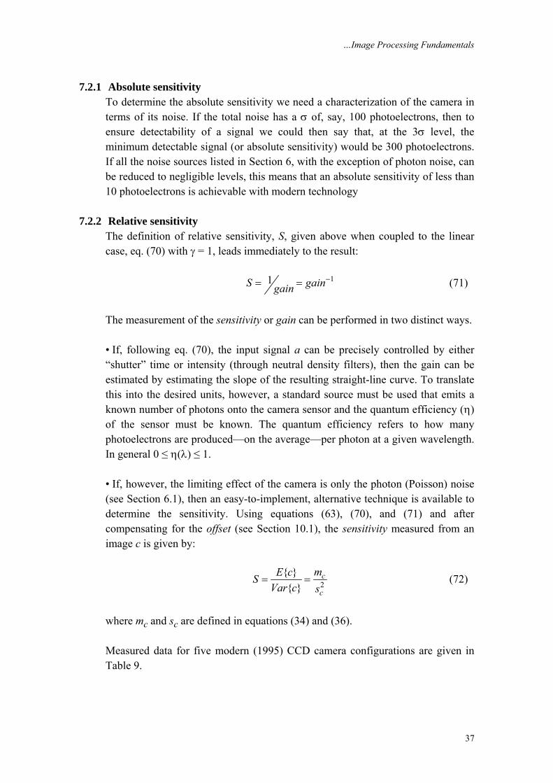
7.2.1 Absolute sensitivity To determine the absolute sensitivity we need a characterization of the camera in terms of its noise. If the total noise has a σ of, say, 100 photoelectrons, then to ensure detectability of a signal we could then say that, at the 3σ level, the minimum detectable signal (or absolute sensitivity) would be 300 photoelectrons. If all the noise sources listed in Section 6, with the exception of photon noise, can be reduced to negligible levels, this means that an absolute sensitivity of less than 10 photoelectrons is achievable with modern technology
7.2.2 Relative sensitivity The definition of relative sensitivity, S, given above when coupled to the linear case, eq. (70) with γ = 1, leads immediately to the result: 11S gaingain
−= = (71)
The measurement of the sensitivity or gain can be performed in two distinct ways. • If, following eq. (70), the input signal a can be precisely controlled by either “shutter” time or intensity (through neutral density filters), then the gain can be estimated by estimating the slope of the resulting straight-line curve. To translate this into the desired units, however, a standard source must be used that emits a known number of photons onto the camera sensor and the quantum efficiency (η) of the sensor must be known. The quantum efficiency refers to how many photoelectrons are produced—on the average—per photon at a given wavelength. In general 0 ≤ η(λ) ≤ 1. • If, however, the limiting effect of the camera is only the photon (Poisson) noise (see Section 6.1), then an easy-to-implement, alternative technique is available to determine the sensitivity. Using equations (63), (70), and (71) and after compensating for the offset (see Section 10.1), the sensitivity measured from an image c is given by:
2{ }{ }
c
c
mE cSVar c s
= = (72)
where mc and sc are defined in equations (34) and (36). Measured data for five modern (1995) CCD camera configurations are given in Table 9.
…Image Processing Fundamentals
38
Camera Pixels Pixel size Temp. S BitsLabel µm x µm K e – / ADU
C–1 1320 x 1035 6.8 x 6.8 231 7.9 12C–2 578 x 385 22.0 x 22.0 227 9.7 16C–3 1320 x 1035 6.8 x 6.8 293 48.1 10C–4 576 x 384 23.0 x 23.0 238 90.9 12C–5 756 x 581 11.0 x 5.5 300 109.2 8
Table 9: Sensitivity measurements. Note that a more sensitive camera has a lower value of S.
The extraordinary sensitivity of modern CCD cameras is clear from these data. In a scientific-grade CCD camera (C–1), only 8 photoelectrons (approximately 16 photons) separate two gray levels in the digital representation of the image. For a considerably less expensive video camera (C–5), only about 110 photoelectrons (approximately 220 photons) separate two gray levels.
7.3 SNR As described in Section 6, in modern camera systems the noise is frequently limited by:
• amplifier noise in the case of color cameras; • thermal noise which, itself, is limited by the chip temperature K and the
exposure time T, and/or; • photon noise which is limited by the photon production rate ρ and the
exposure time T.
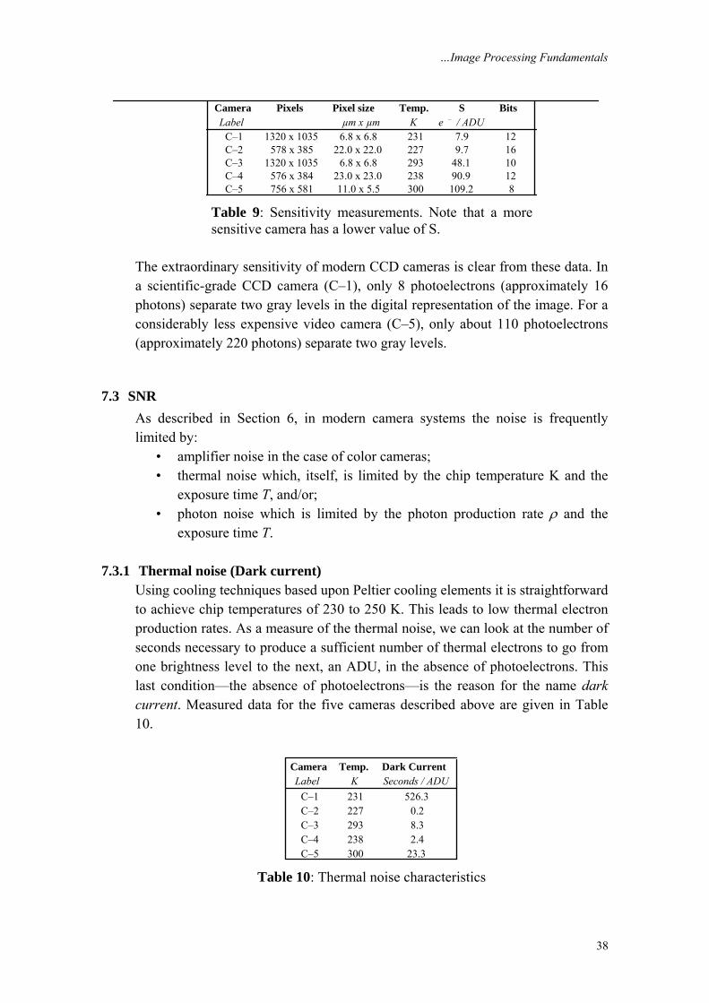
7.3.1 Thermal noise (Dark current) Using cooling techniques based upon Peltier cooling elements it is straightforward to achieve chip temperatures of 230 to 250 K. This leads to low thermal electron production rates. As a measure of the thermal noise, we can look at the number of seconds necessary to produce a sufficient number of thermal electrons to go from one brightness level to the next, an ADU, in the absence of photoelectrons. This last condition—the absence of photoelectrons—is the reason for the name dark current. Measured data for the five cameras described above are given in Table 10.
Camera Temp. Dark CurrentLabel K Seconds / ADU
C–1 231 526.3C–2 227 0.2C–3 293 8.3C–4 238 2.4C–5 300 23.3
Table 10: Thermal noise characteristics
…Image Processing Fundamentals
39
The video camera (C–5) has on-chip dark current suppression. (See Section 6.2.) Operating at room temperature this camera requires more than 20 seconds to produce one ADU change due to thermal noise. This means at the conventional video frame and integration rates of 25 to 30 images per second (see Table 3), the thermal noise is negligible.
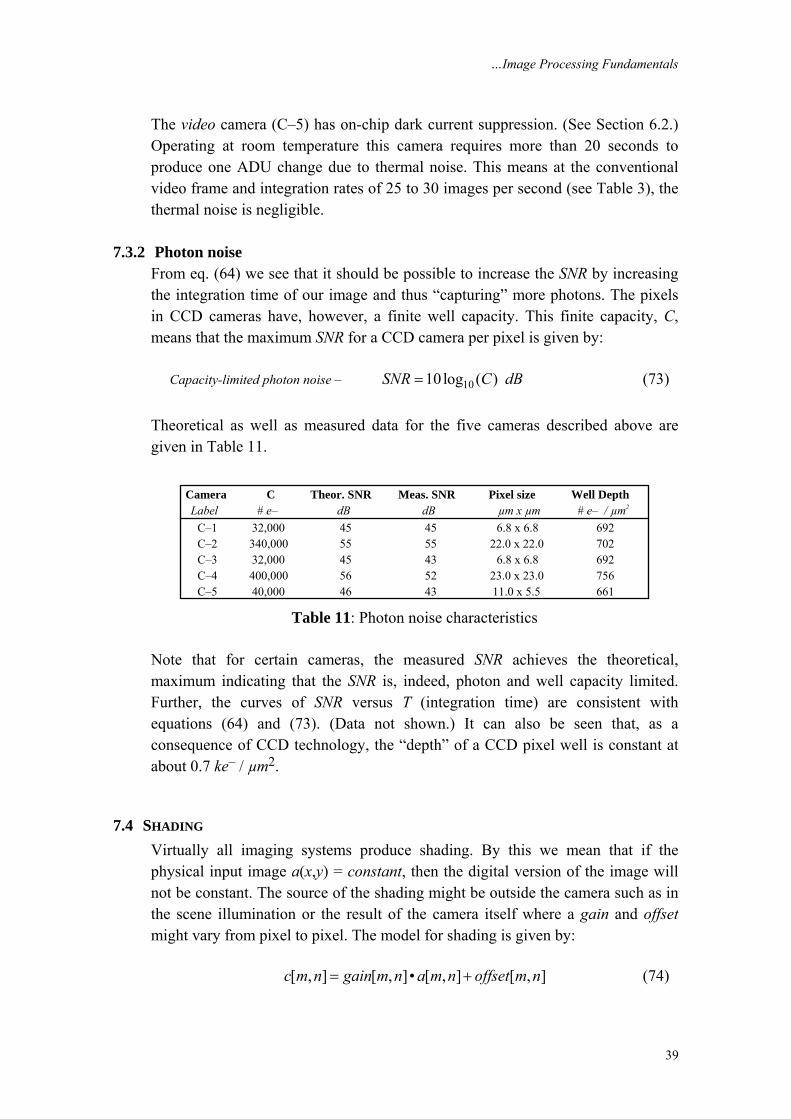
7.3.2 Photon noise From eq. (64) we see that it should be possible to increase the SNR by increasing the integration time of our image and thus “capturing” more photons. The pixels in CCD cameras have, however, a finite well capacity. This finite capacity, C, means that the maximum SNR for a CCD camera per pixel is given by: Capacity-limited photon noise – 1010log ( ) SNR C dB= (73) Theoretical as well as measured data for the five cameras described above are given in Table 11.
Camera C Theor. SNR Meas. SNR Pixel size Well DepthLabel # e– dB dB µm x µm # e– / µm2
C–1 32,000 45 45 6.8 x 6.8 692C–2 340,000 55 55 22.0 x 22.0 702C–3 32,000 45 43 6.8 x 6.8 692C–4 400,000 56 52 23.0 x 23.0 756C–5 40,000 46 43 11.0 x 5.5 661
Table 11: Photon noise characteristics Note that for certain cameras, the measured SNR achieves the theoretical, maximum indicating that the SNR is, indeed, photon and well capacity limited. Further, the curves of SNR versus T (integration time) are consistent with equations (64) and (73). (Data not shown.) It can also be seen that, as a consequence of CCD technology, the “depth” of a CCD pixel well is constant at about 0.7 ke– / µm2.
7.4 SHADING Virtually all imaging systems produce shading. By this we mean that if the physical input image a(x,y) = constant, then the digital version of the image will not be constant. The source of the shading might be outside the camera such as in the scene illumination or the result of the camera itself where a gain and offset might vary from pixel to pixel. The model for shading is given by: [ , ] [ , ]• [ , ] [ , ]c m n gain m n a m n offset m n= + (74)
…Image Processing Fundamentals
40
where a[m,n] is the digital image that would have been recorded if there were no shading in the image, that is, a[m,n] = constant. Techniques for reducing or removing the effects of shading are discussed in Section 10.1.
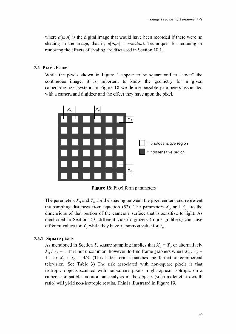
7.5 PIXEL FORM While the pixels shown in Figure 1 appear to be square and to “cover” the continuous image, it is important to know the geometry for a given camera/digitizer system. In Figure 18 we define possible parameters associated with a camera and digitizer and the effect they have upon the pixel.
= photosensitive region
= nonsensitive region
Xo
Yo
Xa
Ya
Figure 18: Pixel form parameters
The parameters Xo and Yo are the spacing between the pixel centers and represent the sampling distances from equation (52). The parameters Xa and Ya are the dimensions of that portion of the camera’s surface that is sensitive to light. As mentioned in Section 2.3, different video digitizers (frame grabbers) can have different values for Xo while they have a common value for Yo.
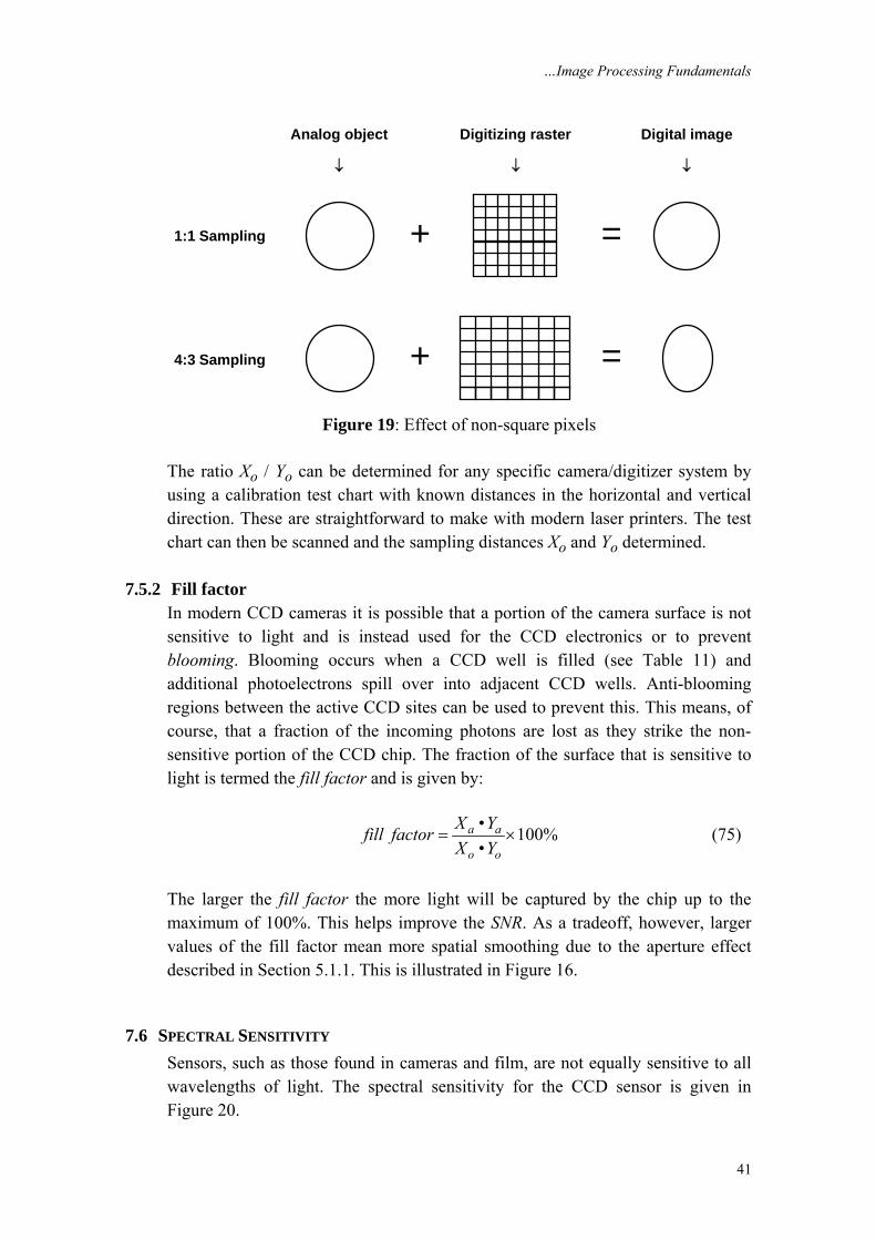
7.5.1 Square pixels As mentioned in Section 5, square sampling implies that Xo = Yo or alternatively Xo / Yo = 1. It is not uncommon, however, to find frame grabbers where Xo / Yo = 1.1 or Xo / Yo = 4/3. (This latter format matches the format of commercial television. See Table 3) The risk associated with non-square pixels is that isotropic objects scanned with non-square pixels might appear isotropic on a camera-compatible monitor but analysis of the objects (such as length-to-width ratio) will yield non-isotropic results. This is illustrated in Figure 19.
…Image Processing Fundamentals
41
Analog object
↓
Digitizing raster
↓
Digital image
↓
+ =1:1 Sampling
4:3 Sampling + =
Figure 19: Effect of non-square pixels The ratio Xo / Yo can be determined for any specific camera/digitizer system by using a calibration test chart with known distances in the horizontal and vertical direction. These are straightforward to make with modern laser printers. The test chart can then be scanned and the sampling distances Xo and Yo determined.
7.5.2 Fill factor In modern CCD cameras it is possible that a portion of the camera surface is not sensitive to light and is instead used for the CCD electronics or to prevent blooming. Blooming occurs when a CCD well is filled (see Table 11) and additional photoelectrons spill over into adjacent CCD wells. Anti-blooming regions between the active CCD sites can be used to prevent this. This means, of course, that a fraction of the incoming photons are lost as they strike the non-sensitive portion of the CCD chip. The fraction of the surface that is sensitive to light is termed the fill factor and is given by:
• 100%•
a a
o o
X Yfill factorX Y
= × (75)
The larger the fill factor the more light will be captured by the chip up to the maximum of 100%. This helps improve the SNR. As a tradeoff, however, larger values of the fill factor mean more spatial smoothing due to the aperture effect described in Section 5.1.1. This is illustrated in Figure 16.
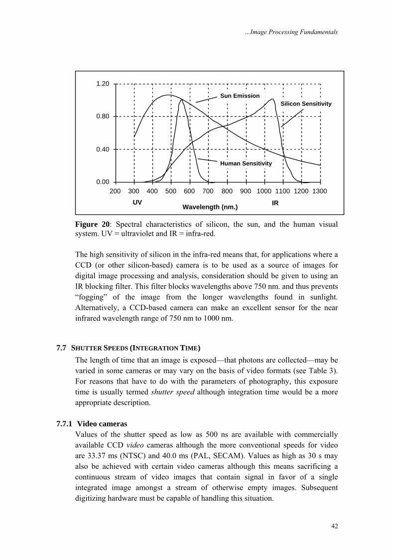
7.6 SPECTRAL SENSITIVITY Sensors, such as those found in cameras and film, are not equally sensitive to all wavelengths of light. The spectral sensitivity for the CCD sensor is given in Figure 20.
…Image Processing Fundamentals
42
0.00
0.40
0.80
1.20
200 300 400 500 600 700 800 900 1000 1100 1200 1300
UV IR
Sun Emission
Human Sensitivity
Silicon Sensitivity
Wavelength (nm.)
Figure 20: Spectral characteristics of silicon, the sun, and the human visual system. UV = ultraviolet and IR = infra-red. The high sensitivity of silicon in the infra-red means that, for applications where a CCD (or other silicon-based) camera is to be used as a source of images for digital image processing and analysis, consideration should be given to using an IR blocking filter. This filter blocks wavelengths above 750 nm. and thus prevents “fogging” of the image from the longer wavelengths found in sunlight. Alternatively, a CCD-based camera can make an excellent sensor for the near infrared wavelength range of 750 nm to 1000 nm.
7.7 SHUTTER SPEEDS (INTEGRATION TIME) The length of time that an image is exposed—that photons are collected—may be varied in some cameras or may vary on the basis of video formats (see Table 3). For reasons that have to do with the parameters of photography, this exposure time is usually termed shutter speed although integration time would be a more appropriate description.
7.7.1 Video cameras Values of the shutter speed as low as 500 ns are available with commercially available CCD video cameras although the more conventional speeds for video are 33.37 ms (NTSC) and 40.0 ms (PAL, SECAM). Values as high as 30 s may also be achieved with certain video cameras although this means sacrificing a continuous stream of video images that contain signal in favor of a single integrated image amongst a stream of otherwise empty images. Subsequent digitizing hardware must be capable of handling this situation.
…Image Processing Fundamentals
43
7.7.2 Scientific cameras Again values as low as 500 ns are possible and, with cooling techniques based on Peltier-cooling or liquid nitrogen cooling, integration times in excess of one hour are readily achieved.
7.8 READOUT RATE The rate at which data is read from the sensor chip is termed the readout rate. The readout rate for standard video cameras depends on the parameters of the frame grabber as well as the camera. For standard video, see Section 2.3, the readout rate is given by:
• •sec
images lines pixelsRimage line
⎛ ⎞⎛ ⎞ ⎛ ⎞= ⎜ ⎟⎜ ⎟ ⎜ ⎟⎝ ⎠ ⎝ ⎠⎝ ⎠
(76)
While the appropriate unit for describing the readout rate should be pixels / second, the term Hz is frequently found in the literature and in camera specifications; we shall therefore use the latter unit. For a video camera with square pixels (see Section 7.5), this means:
Format lines / sec pixels / line R (MHz.) NTSC 15,750 (4/3)*525 ≈11.0 PAL / SECAM 15,625 (4/3)*625 ≈13.0
Table 12: Video camera readout rates Note that the values in Table 12 are approximate. Exact values for square-pixel systems require exact knowledge of the way the video digitizer (frame grabber) samples each video line. The readout rates used in video cameras frequently means that the electronic noise described in Section 6.3 occurs in the region of the noise spectrum (eq. (65)) described by ω > ωmax where the noise power increases with increasing frequency. Readout noise can thus be significant in video cameras. Scientific cameras frequently use a slower readout rate in order to reduce the readout noise. Typical values of readout rate for scientific cameras, such as those described in Tables 9, 10, and 11, are 20 kHz, 500 kHz, and 1 MHz to 8 MHz.
…Image Processing Fundamentals
44
8. Displays The displays used for image processing—particularly the display systems used with computers—have a number of characteristics that help determine the quality of the final image.
8.1 REFRESH RATE The refresh rate is defined as the number of complete images that are written to the screen per second. For standard video the refresh rate is fixed at the values given in Table 3, either 29.97 or 25 images/s. For computer displays the refresh rate can vary with common values being 67 images/s and 75 images/s. At values above 60 images/s visual flicker is negligible at virtually all illumination levels.
8.2 INTERLACING To prevent the appearance of visual flicker at refresh rates below 60 images/s, the display can be interlaced as described in Section 2.3. Standard interlace for video systems is 2:1. Since interlacing is not necessary at refresh rates above 60 images/s, an interlace of 1:1 is used with such systems. In other words, lines are drawn in an ordinary sequential fashion: 1,2,3,4,…,N.
8.3 RESOLUTION The pixels stored in computer memory, although they are derived from regions of finite area in the original scene (see Sections 5.1 and 7.5), may be thought of as mathematical points having no physical extent. When displayed, the space between the points must be filled in. This generally happens as a result of the finite spot size of a cathode-ray tube (CRT). The brightness profile of a CRT spot is approximately Gaussian and the number of spots that can be resolved on the display depends on the quality of the system. It is relatively straightforward to obtain display systems with a resolution of 72 spots per inch (28.3 spots per cm.) This number corresponds to standard printing conventions. If printing is not a consideration then higher resolutions, in excess of 30 spots per cm, are attainable.
9. Algorithms In this Section we will describe operations that are fundamental to digital image processing. These operations can be divided into four categories: operations based on the image histogram, on simple mathematics, on convolution, and on mathematical morphology. Further, these operations can also be described in
…Image Processing Fundamentals
45
terms of their implementation as a point operation, a local operation, or a global operation as described in Section 2.2.1.
9.1 HISTOGRAM-BASED OPERATIONS An important class of point operations is based upon the manipulation of an image histogram or a region histogram. The most important examples are described below.
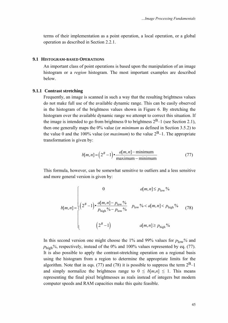
9.1.1 Contrast stretching Frequently, an image is scanned in such a way that the resulting brightness values do not make full use of the available dynamic range. This can be easily observed in the histogram of the brightness values shown in Figure 6. By stretching the histogram over the available dynamic range we attempt to correct this situation. If the image is intended to go from brightness 0 to brightness 2B–1 (see Section 2.1), then one generally maps the 0% value (or minimum as defined in Section 3.5.2) to the value 0 and the 100% value (or maximum) to the value 2B–1. The appropriate transformation is given by:
( ) [ , ] minimum[ , ] 2 1 •maximum minimum
B a m nb m n −= −
− (77)
This formula, however, can be somewhat sensitive to outliers and a less sensitive and more general version is given by:
( )
( )
low
lowlow high
high low
high
0 [ , ] %
[ , ] %2 1 • % [ , ] %[ , ] % %
2 1 [ , ] %
B
B
a m n p
a m n p p a m n pb m n p p
a m n p
≤⎧⎪⎪⎪ −⎪ − < <= ⎨ −⎪⎪⎪
− ≥⎪⎩
(78)
In this second version one might choose the 1% and 99% values for plow% and phigh%, respectively, instead of the 0% and 100% values represented by eq. (77). It is also possible to apply the contrast-stretching operation on a regional basis using the histogram from a region to determine the appropriate limits for the algorithm. Note that in eqs. (77) and (78) it is possible to suppress the term 2B–1 and simply normalize the brightness range to 0 ≤ b[m,n] ≤ 1. This means representing the final pixel brightnesses as reals instead of integers but modern computer speeds and RAM capacities make this quite feasible.
…Image Processing Fundamentals
46
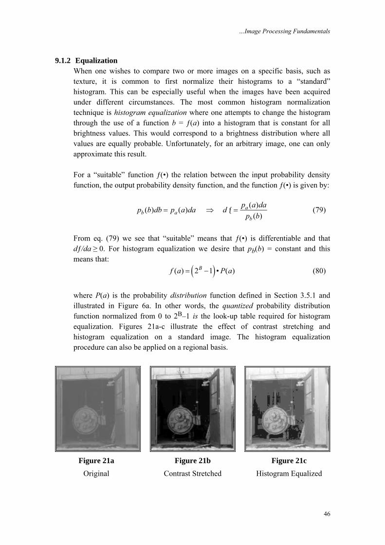
9.1.2 Equalization When one wishes to compare two or more images on a specific basis, such as texture, it is common to first normalize their histograms to a “standard” histogram. This can be especially useful when the images have been acquired under different circumstances. The most common histogram normalization technique is histogram equalization where one attempts to change the histogram through the use of a function b = ƒ(a) into a histogram that is constant for all brightness values. This would correspond to a brightness distribution where all values are equally probable. Unfortunately, for an arbitrary image, one can only approximate this result. For a “suitable” function ƒ(•) the relation between the input probability density function, the output probability density function, and the function ƒ(•) is given by:
( )( ) ( )( )
ab a
b
p a dap b db p a da dp b
= ⇒ ƒ = (79)
From eq. (79) we see that “suitable” means that ƒ(•) is differentiable and that dƒ/da ≥ 0. For histogram equalization we desire that pb(b) = constant and this means that: ( )( ) 2 1 • ( )Bf a P a= − (80)
where P(a) is the probability distribution function defined in Section 3.5.1 and illustrated in Figure 6a. In other words, the quantized probability distribution function normalized from 0 to 2B–1 is the look-up table required for histogram equalization. Figures 21a-c illustrate the effect of contrast stretching and histogram equalization on a standard image. The histogram equalization procedure can also be applied on a regional basis.
Figure 21a Figure 21b Figure 21c
Original Contrast Stretched Histogram Equalized
…Image Processing Fundamentals
47
9.1.3 Other histogram-based operations The histogram derived from a local region can also be used to drive local filters that are to be applied to that region. Examples include minimum filtering, median filtering, and maximum filtering [23]. The concepts minimum, median, and maximum were introduced in Figure 6. The filters based on these concepts will be presented formally in Sections 9.4.2 and 9.6.10.
9.2 MATHEMATICS-BASED OPERATIONS We distinguish in this section between binary arithmetic and ordinary arithmetic. In the binary case there are two brightness values “0” and “1”. In the ordinary case we begin with 2B brightness values or levels but the processing of the image can easily generate many more levels. For this reason many software systems provide 16 or 32 bit representations for pixel brightnesses in order to avoid problems with arithmetic overflow.
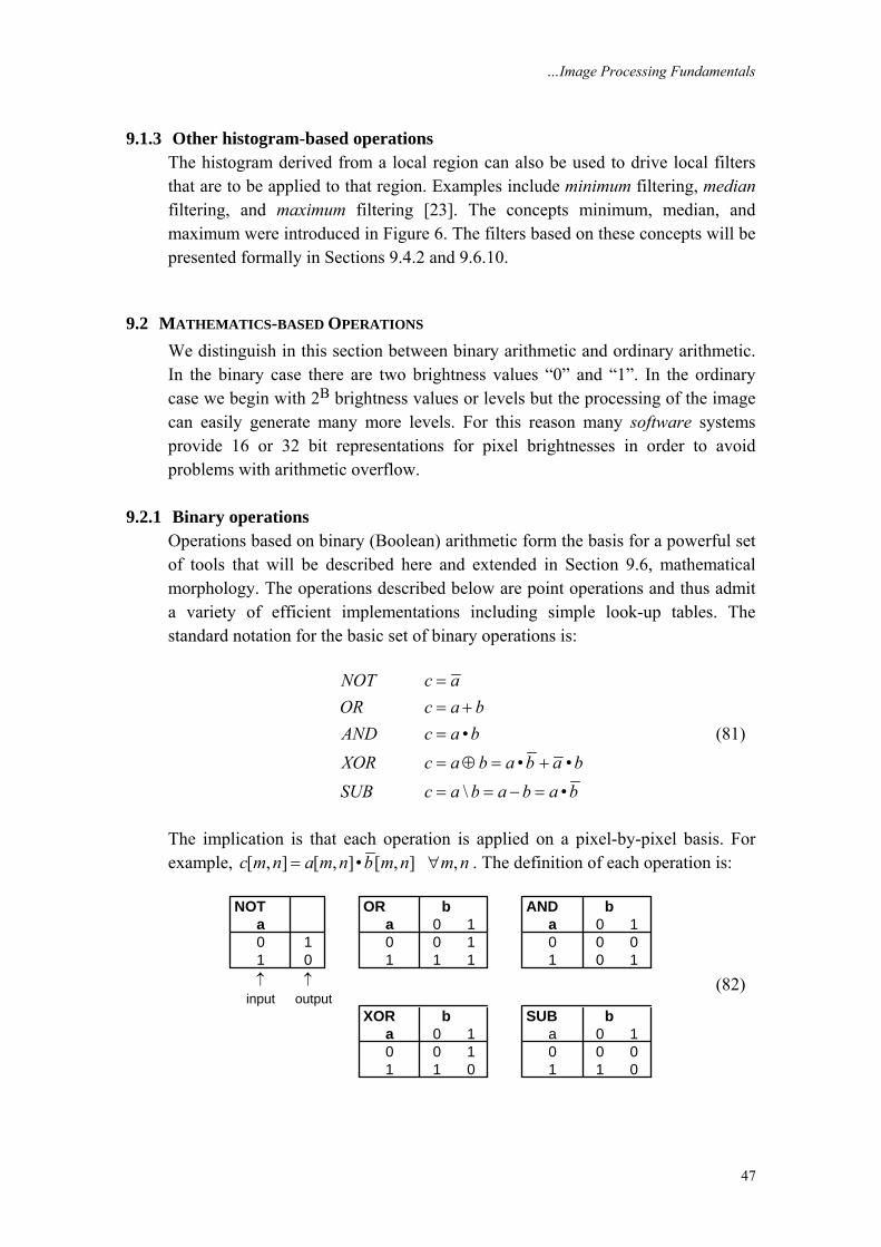
9.2.1 Binary operations Operations based on binary (Boolean) arithmetic form the basis for a powerful set of tools that will be described here and extended in Section 9.6, mathematical morphology. The operations described below are point operations and thus admit a variety of efficient implementations including simple look-up tables. The standard notation for the basic set of binary operations is:
•• •
\ •
NOT c aOR c a bAND c a bXOR c a b a b a bSUB c a b a b a b
== +=
= ⊕ = +
= = − =
(81)
The implication is that each operation is applied on a pixel-by-pixel basis. For example, [ , ] [ , ]• [ , ] ,c m n a m n b m n m n= ∀ . The definition of each operation is:
NOT OR b AND ba a 0 1 a 0 10 1 0 0 1 0 0 01 0 1 1 1 1 0 1↑ ↑
input outputXOR b SUB b
a 0 1 a 0 10 0 1 0 0 01 1 0 1 1 0
(82)
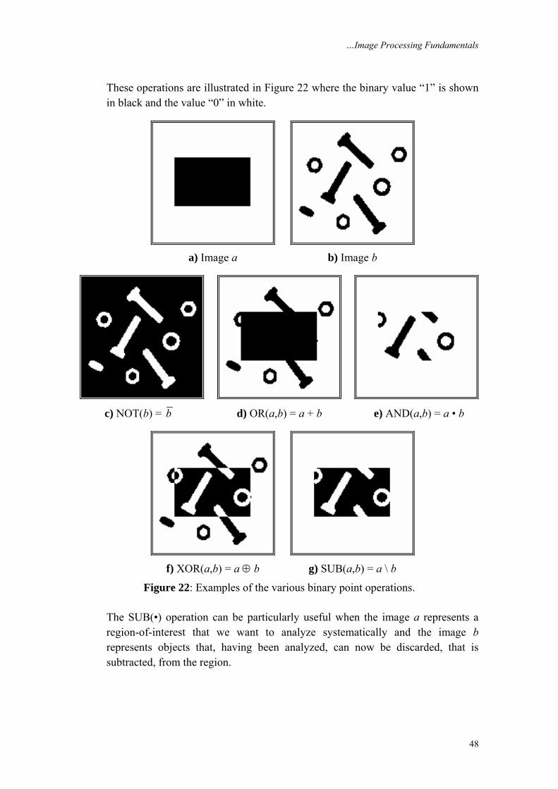
…Image Processing Fundamentals
48
These operations are illustrated in Figure 22 where the binary value “1” is shown in black and the value “0” in white.
a) Image a b) Image b
c) NOT(b) = b d) OR(a,b) = a + b e) AND(a,b) = a • b
f) XOR(a,b) = a ⊕ b g) SUB(a,b) = a \ b
Figure 22: Examples of the various binary point operations. The SUB(•) operation can be particularly useful when the image a represents a region-of-interest that we want to analyze systematically and the image b represents objects that, having been analyzed, can now be discarded, that is subtracted, from the region.
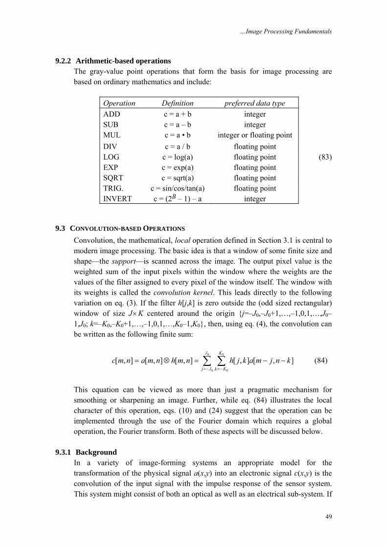
…Image Processing Fundamentals
49
9.2.2 Arithmetic-based operations The gray-value point operations that form the basis for image processing are based on ordinary mathematics and include:
Operation Definition preferred data type ADD c = a + b integer SUB c = a – b integer MUL c = a • b integer or floating point DIV c = a / b floating point LOG c = log(a) floating point (83)EXP c = exp(a) floating point SQRT c = sqrt(a) floating point TRIG. c = sin/cos/tan(a) floating point INVERT c = (2B – 1) – a integer
9.3 CONVOLUTION-BASED OPERATIONS Convolution, the mathematical, local operation defined in Section 3.1 is central to modern image processing. The basic idea is that a window of some finite size and shape—the support—is scanned across the image. The output pixel value is the weighted sum of the input pixels within the window where the weights are the values of the filter assigned to every pixel of the window itself. The window with its weights is called the convolution kernel. This leads directly to the following variation on eq. (3). If the filter h[j,k] is zero outside the (odd sized rectangular) window of size J×K centered around the origin {j=–J0,–J0+1,…,–1,0,1,…,J0–1,J0; k=–K0,–K0+1,…,–1,0,1,…,K0–1,K0}, then, using eq. (4), the convolution can be written as the following finite sum:
0 0
0 0
[ , ] [ , ] [ , ] [ , ] [ , ]J K
j J k Kc m n a m n h m n h j k a m j n k
=− =−
= ⊗ = − −∑ ∑ (84)
This equation can be viewed as more than just a pragmatic mechanism for smoothing or sharpening an image. Further, while eq. (84) illustrates the local character of this operation, eqs. (10) and (24) suggest that the operation can be implemented through the use of the Fourier domain which requires a global operation, the Fourier transform. Both of these aspects will be discussed below.
9.3.1 Background In a variety of image-forming systems an appropriate model for the transformation of the physical signal a(x,y) into an electronic signal c(x,y) is the convolution of the input signal with the impulse response of the sensor system. This system might consist of both an optical as well as an electrical sub-system. If
…Image Processing Fundamentals
50
each of these systems can be treated as a linear, shift-invariant (LSI) system then the convolution model is appropriate. The definitions of these two, possible, system properties are given below:
Linearity – 1 1 2 2
1 1 2 2 1 1 2 2• • • •If a c and a cThen w a w a w c w c
→ →+ → +
(85)
Shift-Invariance – ( ) ( )( ) ( )
, ,
, ,o o o o
If a x y c x y
Then a x x y y c x x y y
→
− − → − − (86)
where w1 and w2 are arbitrary complex constants and xo and yo are coordinates corresponding to arbitrary spatial translations. Two remarks are appropriate at this point. First, linearity implies (by choosing w1 = w2 = 0) that “zero in” gives “zero out”. The offset described in eq. (70) means that such camera signals are not the output of a linear system and thus (strictly speaking) the convolution result is not applicable. Fortunately, it is straightforward to correct for this non-linear effect. (See Section 10.1.) Second, optical lenses with a magnification, M, other than 1× are not shift invariant; a translation of 1 unit in the input image a(x,y) produces a translation of M units in the output image c(x,y). Due to the Fourier property described in eq. (25) this case can still be handled by linear system theory. If an impulse point of light δ(x,y) is imaged through an LSI system then the impulse response of that system is called the point spread function (PSF). The output image then becomes the convolution of the input image with the PSF. The Fourier transform of the PSF is called the optical transfer function (OTF). For optical systems that are circularly-symmetric, aberration-free, and diffraction-limited the PSF is given by the Airy disk shown in Table 4–T.5. The OTF of the Airy disk is also presented in Table 4–T.5. If the convolution window is not the diffraction-limited PSF of the lens but rather the effect of defocusing a lens then an appropriate model for h(x,y) is a pill box of radius a as described in Table 4–T.3. The effect on a test pattern is illustrated in Figure 23.
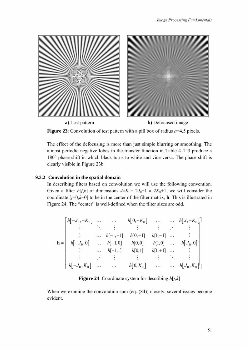
…Image Processing Fundamentals
51
a) Test pattern b) Defocused image
Figure 23: Convolution of test pattern with a pill box of radius a=4.5 pixels. The effect of the defocusing is more than just simple blurring or smoothing. The almost periodic negative lobes in the transfer function in Table 4–T.3 produce a 180° phase shift in which black turns to white and vice-versa. The phase shift is clearly visible in Figure 23b.
9.3.2 Convolution in the spatial domain In describing filters based on convolution we will use the following convention. Given a filter h[j,k] of dimensions J×K = 2J0+1 × 2K0+1, we will consider the coordinate [j=0,k=0] to be in the center of the filter matrix, h. This is illustrated in Figure 24. The “center” is well-defined when the filter sizes are odd.
[ ] [ ] [ ]
[ ] [ ]
[ ] [ ] [ ]
0 0 0 0
0 0
0 0 0 0 0
, 0, ,
[ 1, 1] [0, 1] [1, 1],0 [ 1,0] [0,0] [1,0] ,0
[ 1,1] [0,1] [1, 1]
, 0, ,
h J K h K h J K
h h hh J h h h h J
h h h
h J K h K h J K
⎡ ⎤− − … … − … … −⎢ ⎥⎢ ⎥⎢ ⎥… − − − − …⎢ ⎥
= − … − …⎢ ⎥⎢ ⎥… − + …⎢ ⎥⎢ ⎥⎢ ⎥− … … … …⎣ ⎦
h
Figure 24: Coordinate system for describing h[j,k] When we examine the convolution sum (eq. (84)) closely, several issues become evident.
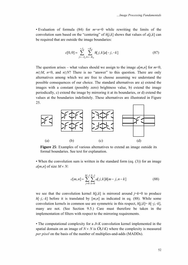
…Image Processing Fundamentals
52
• Evaluation of formula (84) for m=n=0 while rewriting the limits of the convolution sum based on the “centering” of h[j,k] shows that values of a[j,k] can be required that are outside the image boundaries:
0 0
0 0
[0,0] [ , ] [ , ]J K
j J k Kc h j k a j k
+ +
=− =−
= − −∑ ∑ (87)
The question arises – what values should we assign to the image a[m,n] for m<0, m≥M, n<0, and n≥N? There is no “answer” to this question. There are only alternatives among which we are free to choose assuming we understand the possible consequences of our choice. The standard alternatives are a) extend the images with a constant (possibly zero) brightness value, b) extend the image periodically, c) extend the image by mirroring it at its boundaries, or d) extend the values at the boundaries indefinitely. These alternatives are illustrated in Figure 25.
(a) (b) (c) (d)
Figure 25: Examples of various alternatives to extend an image outside its formal boundaries. See text for explanation.
• When the convolution sum is written in the standard form (eq. (3)) for an image a[m,n] of size M × N:
1 1
0 0[ , ] [ , ] [ , ]
M N
j kc m n a j k h m j n k
− −
= == − −∑ ∑ (88)
we see that the convolution kernel h[j,k] is mirrored around j=k=0 to produce h[–j,–k] before it is translated by [m,n] as indicated in eq. (88). While some convolution kernels in common use are symmetric in this respect, h[j,k]= h[–j,–k], many are not. (See Section 9.5.) Care must therefore be taken in the implementation of filters with respect to the mirroring requirements. • The computational complexity for a J×K convolution kernel implemented in the spatial domain on an image of N × N is O(J⋅K) where the complexity is measured per pixel on the basis of the number of multiplies-and-adds (MADDs).
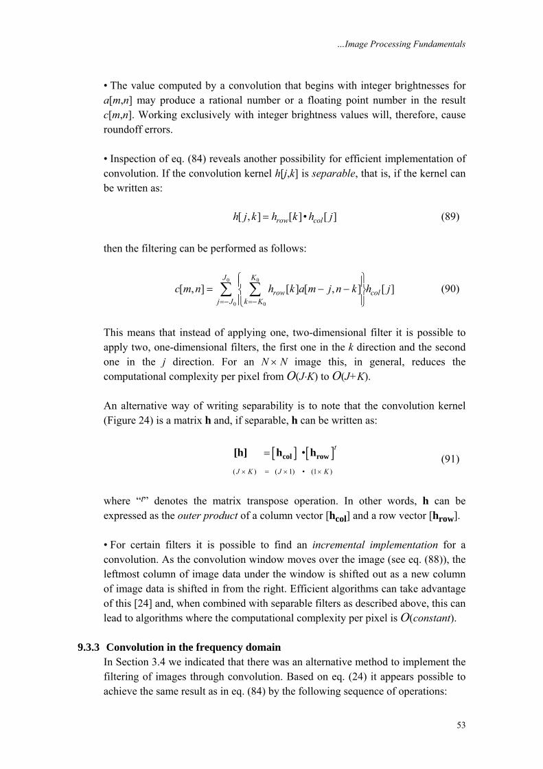
…Image Processing Fundamentals
53
• The value computed by a convolution that begins with integer brightnesses for a[m,n] may produce a rational number or a floating point number in the result c[m,n]. Working exclusively with integer brightness values will, therefore, cause roundoff errors. • Inspection of eq. (84) reveals another possibility for efficient implementation of convolution. If the convolution kernel h[j,k] is separable, that is, if the kernel can be written as: [ , ] [ ]• [ ]row colh j k h k h j= (89) then the filtering can be performed as follows:
0 0
0 0
[ , ] [ ] [ , ] [ ]J K
row colj J k K
c m n h k a m j n k h j=− =−
⎧ ⎫⎪ ⎪= − −⎨ ⎬⎪ ⎪⎩ ⎭
∑ ∑ (90)
This means that instead of applying one, two-dimensional filter it is possible to apply two, one-dimensional filters, the first one in the k direction and the second one in the j direction. For an N × N image this, in general, reduces the computational complexity per pixel from O(J⋅K) to O(J+K). An alternative way of writing separability is to note that the convolution kernel (Figure 24) is a matrix h and, if separable, h can be written as:
[ ] [ ]( ) ( 1) • (1 )
•J K J K
t
× = × ×
= col row[h] h h (91)
where “t” denotes the matrix transpose operation. In other words, h can be expressed as the outer product of a column vector [hcol] and a row vector [hrow]. • For certain filters it is possible to find an incremental implementation for a convolution. As the convolution window moves over the image (see eq. (88)), the leftmost column of image data under the window is shifted out as a new column of image data is shifted in from the right. Efficient algorithms can take advantage of this [24] and, when combined with separable filters as described above, this can lead to algorithms where the computational complexity per pixel is O(constant).
9.3.3 Convolution in the frequency domain In Section 3.4 we indicated that there was an alternative method to implement the filtering of images through convolution. Based on eq. (24) it appears possible to achieve the same result as in eq. (84) by the following sequence of operations:
…Image Processing Fundamentals
54
i) Compute A(Ω,Ψ) = F{a[m,n]} ii) Multiply A(Ω,Ψ) by the precomputed H(Ω,Ψ) = F{h[m,n]} (92) iii) Compute the result c[m,n] = F–1{A(Ω,Ψ)•H(Ω,Ψ)} • While it might seem that the “recipe” given above in eq. (92) circumvents the problems associated with direct convolution in the spatial domain—specifically, determining values for the image outside the boundaries of the image—the Fourier domain approach, in fact, simply “assumes” that the image is repeated periodically outside its boundaries as illustrated in Figure 25b. This phenomenon is referred to as circular convolution. If circular convolution is not acceptable then the other possibilities illustrated in Figure 25 can be realized by embedding the image a[m,n] and the filter H(Ω,Ψ) in larger matrices with the desired image extension mechanism for a[m,n] being explicitly implemented. • The computational complexity per pixel of the Fourier approach for an image of N × N and for a convolution kernel of K × K is O(2logN) complex MADDs independent of K. Here we assume that N > K and that N is a highly composite number such as a power of two. (See also 2.1.) This latter assumption permits use of the computationally-efficient Fast Fourier Transform (FFT) algorithm. Surprisingly then, the indirect route described by eq. (92) can be faster than the direct route given in eq. (84). This requires, in general, that K2 >> 2logN. The range of K and N for which this holds depends on the specifics of the implementation. For the machine on which this manuscript is being written and the specific image processing package that is being used, for an image of N = 256 the Fourier approach is faster than the convolution approach when K ≥ 15. (It should be noted that in this comparison the direct convolution involves only integer arithmetic while the Fourier domain approach requires complex floating point arithmetic.)
9.4 SMOOTHING OPERATIONS These algorithms are applied in order to reduce noise and/or to prepare images for further processing such as segmentation. We distinguish between linear and non- linear algorithms where the former are amenable to analysis in the Fourier domain and the latter are not. We also distinguish between implementations based on a rectangular support for the filter and implementations based on a circular support for the filter.
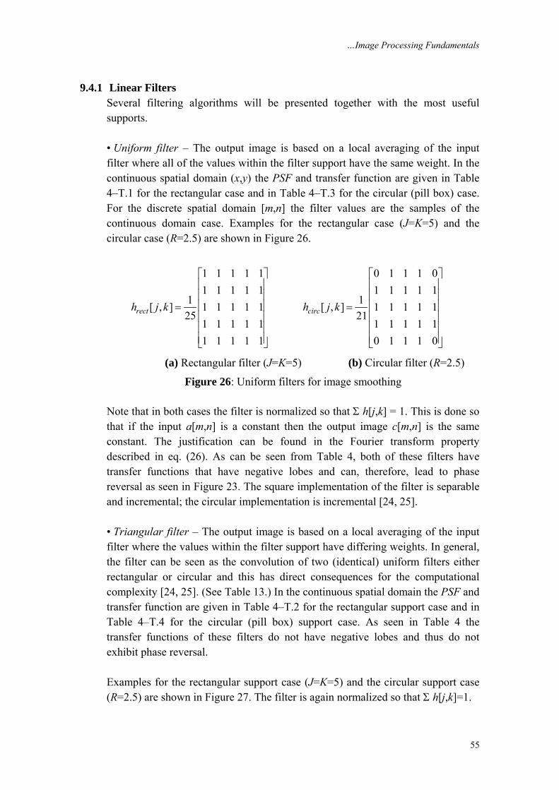
…Image Processing Fundamentals
55
9.4.1 Linear Filters Several filtering algorithms will be presented together with the most useful supports. • Uniform filter – The output image is based on a local averaging of the input filter where all of the values within the filter support have the same weight. In the continuous spatial domain (x,y) the PSF and transfer function are given in Table 4–T.1 for the rectangular case and in Table 4–T.3 for the circular (pill box) case. For the discrete spatial domain [m,n] the filter values are the samples of the continuous domain case. Examples for the rectangular case (J=K=5) and the circular case (R=2.5) are shown in Figure 26.
1 1 1 1 11 1 1 1 1
1[ , ] 1 1 1 1 125
1 1 1 1 11 1 1 1 1
recth j k
⎡ ⎤⎢ ⎥⎢ ⎥⎢ ⎥=⎢ ⎥⎢ ⎥⎢ ⎥⎣ ⎦
0 1 1 1 01 1 1 1 1
1[ , ] 1 1 1 1 121
1 1 1 1 10 1 1 1 0
circh j k
⎡ ⎤⎢ ⎥⎢ ⎥⎢ ⎥=⎢ ⎥⎢ ⎥⎢ ⎥⎣ ⎦
(a) Rectangular filter (J=K=5) (b) Circular filter (R=2.5)
Figure 26: Uniform filters for image smoothing Note that in both cases the filter is normalized so that Σ h[j,k] = 1. This is done so that if the input a[m,n] is a constant then the output image c[m,n] is the same constant. The justification can be found in the Fourier transform property described in eq. (26). As can be seen from Table 4, both of these filters have transfer functions that have negative lobes and can, therefore, lead to phase reversal as seen in Figure 23. The square implementation of the filter is separable and incremental; the circular implementation is incremental [24, 25]. • Triangular filter – The output image is based on a local averaging of the input filter where the values within the filter support have differing weights. In general, the filter can be seen as the convolution of two (identical) uniform filters either rectangular or circular and this has direct consequences for the computational complexity [24, 25]. (See Table 13.) In the continuous spatial domain the PSF and transfer function are given in Table 4–T.2 for the rectangular support case and in Table 4–T.4 for the circular (pill box) support case. As seen in Table 4 the transfer functions of these filters do not have negative lobes and thus do not exhibit phase reversal. Examples for the rectangular support case (J=K=5) and the circular support case (R=2.5) are shown in Figure 27. The filter is again normalized so that Σ h[j,k]=1.
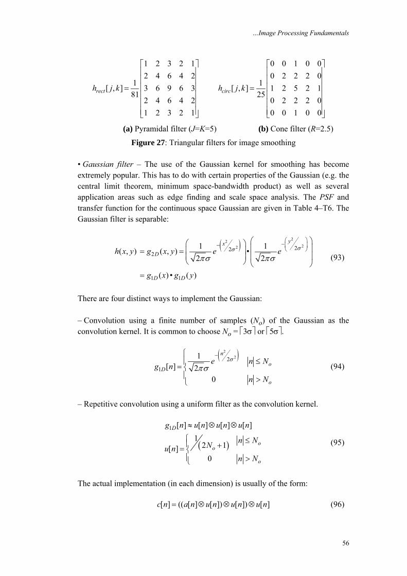
…Image Processing Fundamentals
56
1 2 3 2 12 4 6 4 2
1[ , ] 3 6 9 6 381
2 4 6 4 21 2 3 2 1
recth j k
⎡ ⎤⎢ ⎥⎢ ⎥⎢ ⎥=⎢ ⎥⎢ ⎥⎢ ⎥⎣ ⎦
0 0 1 0 00 2 2 2 0
1[ , ] 1 2 5 2 125
0 2 2 2 00 0 1 0 0
circh j k
⎡ ⎤⎢ ⎥⎢ ⎥⎢ ⎥=⎢ ⎥⎢ ⎥⎢ ⎥⎣ ⎦
(a) Pyramidal filter (J=K=5) (b) Cone filter (R=2.5)
Figure 27: Triangular filters for image smoothing • Gaussian filter – The use of the Gaussian kernel for smoothing has become extremely popular. This has to do with certain properties of the Gaussian (e.g. the central limit theorem, minimum space-bandwidth product) as well as several application areas such as edge finding and scale space analysis. The PSF and transfer function for the continuous space Gaussian are given in Table 4–T6. The Gaussian filter is separable:
( ) 22
22 222
1 1
1 1( , ) ( , ) •2 2
( ) • ( )
yx
D
D D
h x y g x y e e
g x g y
σσ
πσ πσ
⎛ ⎞−− ⎜ ⎟
⎝ ⎠⎛ ⎞⎛ ⎞ ⎜ ⎟= = ⎜ ⎟
⎜ ⎟ ⎜ ⎟⎝ ⎠ ⎝ ⎠=
(93)
There are four distinct ways to implement the Gaussian: – Convolution using a finite number of samples (No) of the Gaussian as the convolution kernel. It is common to choose No = ⎡3σ⎤ or ⎡5σ⎤.
( )2
22
1
1[ ] 2
0
n
oD
o
e n Ng nn N
σ
πσ
−⎧≤⎪= ⎨
⎪ >⎩
(94)
– Repetitive convolution using a uniform filter as the convolution kernel.
( )
1 [ ] [ ] [ ] [ ]1
2 1[ ]0
D
oo
o
g n u n u n u n
n NNu nn N
≈ ⊗ ⊗
⎧ ≤⎪ += ⎨⎪ >⎩
(95)
The actual implementation (in each dimension) is usually of the form: [ ] (( [ ] [ ]) [ ]) [ ]c n a n u n u n u n= ⊗ ⊗ ⊗ (96)
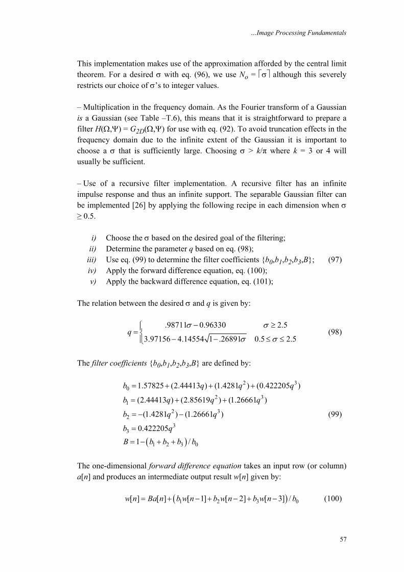
…Image Processing Fundamentals
57
This implementation makes use of the approximation afforded by the central limit theorem. For a desired σ with eq. (96), we use No = ⎡σ⎤ although this severely restricts our choice of σ’s to integer values. – Multiplication in the frequency domain. As the Fourier transform of a Gaussian is a Gaussian (see Table –T.6), this means that it is straightforward to prepare a filter H(Ω,Ψ) = G2D(Ω,Ψ) for use with eq. (92). To avoid truncation effects in the frequency domain due to the infinite extent of the Gaussian it is important to choose a σ that is sufficiently large. Choosing σ > k/π where k = 3 or 4 will usually be sufficient. – Use of a recursive filter implementation. A recursive filter has an infinite impulse response and thus an infinite support. The separable Gaussian filter can be implemented [26] by applying the following recipe in each dimension when σ ≥ 0.5. i) Choose the σ based on the desired goal of the filtering; ii) Determine the parameter q based on eq. (98); iii) Use eq. (99) to determine the filter coefficients {b0,b1,b2,b3,B}; (97) iv) Apply the forward difference equation, eq. (100); v) Apply the backward difference equation, eq. (101); The relation between the desired σ and q is given by:
.98711 0.96330 2.5
3.97156 4.14554 1 .26891 0.5 2.5q
σ σ
σ σ
− ≥⎧⎪= ⎨− − ≤ ≤⎪⎩
(98)
The filter coefficients {b0,b1,b2,b3,B} are defined by:
( )
2 30
2 31
2 32
33
1 2 3 0
1.57825 (2.44413 ) (1.4281 ) (0.422205 )
(2.44413 ) (2.85619 ) (1.26661 )
(1.4281 ) (1.26661 )
0.4222051 /
b q q q
b q q q
b q q
b qB b b b b
= + + +
= + +
= − −
=
= − + +
(99)
The one-dimensional forward difference equation takes an input row (or column) a[n] and produces an intermediate output result w[n] given by: ( )1 2 3 0[ ] [ ] [ 1] [ 2] [ 3] /w n Ba n b w n b w n b w n b= + − + − + − (100)
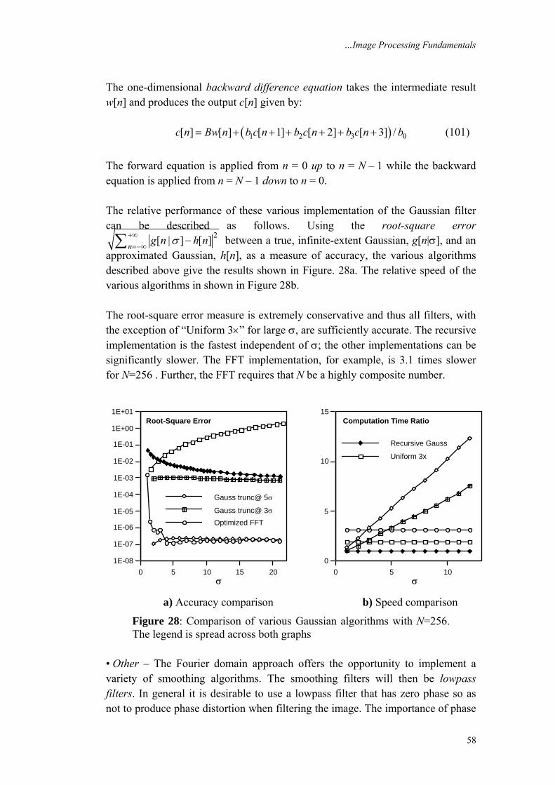
…Image Processing Fundamentals
58
The one-dimensional backward difference equation takes the intermediate result w[n] and produces the output c[n] given by: ( )1 2 3 0[ ] [ ] [ 1] [ 2] [ 3] /c n Bw n b c n b c n b c n b= + + + + + + (101)
The forward equation is applied from n = 0 up to n = N – 1 while the backward equation is applied from n = N – 1 down to n = 0. The relative performance of these various implementation of the Gaussian filter can be described as follows. Using the root-square error
2[ | ] [ ]n g n h nσ+∞=−∞
−∑ between a true, infinite-extent Gaussian, g[n|σ], and an approximated Gaussian, h[n], as a measure of accuracy, the various algorithms described above give the results shown in Figure. 28a. The relative speed of the various algorithms in shown in Figure 28b. The root-square error measure is extremely conservative and thus all filters, with the exception of “Uniform 3×” for large σ, are sufficiently accurate. The recursive implementation is the fastest independent of σ; the other implementations can be significantly slower. The FFT implementation, for example, is 3.1 times slower for N=256 . Further, the FFT requires that N be a highly composite number.
1E-08
1E-07
1E-06
1E-05
1E-04
1E-03
1E-02
1E-01
1E+00
1E+01Root-Square Error
0 5 10 15 20σ
0
5
10
15Computation Time Ratio
0 5 10σ
Optimized FFT
Uniform 3x
Gauss trunc@ 5σ
Gauss trunc@ 3σ
Recursive Gauss
a) Accuracy comparison b) Speed comparison
Figure 28: Comparison of various Gaussian algorithms with N=256. The legend is spread across both graphs
• Other – The Fourier domain approach offers the opportunity to implement a variety of smoothing algorithms. The smoothing filters will then be lowpass filters. In general it is desirable to use a lowpass filter that has zero phase so as not to produce phase distortion when filtering the image. The importance of phase
…Image Processing Fundamentals
59
was illustrated in Figures 5 and 23. When the frequency domain characteristics can be represented in an analytic form, then this can lead to relatively straightforward implementations of H(Ω,Ψ). Possible candidates include the lowpass filters “Airy” and “Exponential Decay” found in Table 4–T.5 and Table 4–T.8, respectively.
9.4.2 Non-Linear Filters A variety of smoothing filters have been developed that are not linear. While they cannot, in general, be submitted to Fourier analysis, their properties and domains of application have been studied extensively. • Median filter – The median statistic was described in Section 3.5.2. A median filter is based upon moving a window over an image (as in a convolution) and computing the output pixel as the median value of the brightnesses within the input window. If the window is J × K in size we can order the J•K pixels in brightness value from smallest to largest. If J•K is odd then the median will be the (J•K+1)/2 entry in the list of ordered brightnesses. Note that the value selected will be exactly equal to one of the existing brightnesses so that no roundoff error will be involved if we want to work exclusively with integer brightness values. The algorithm as it is described above has a generic complexity per pixel of O(J•K•log(J•K)). Fortunately, a fast algorithm (due to Huang et al. [23]) exists that reduces the complexity to O(K) assuming J ≥ K. A useful variation on the theme of the median filter is the percentile filter. Here the center pixel in the window is replaced not by the 50% (median) brightness value but rather by the p% brightness value where p% ranges from 0% (the minimum filter) to 100% (the maximum filter). Values other then (p=50)% do not, in general, correspond to smoothing filters. • Kuwahara filter – Edges play an important role in our perception of images (see Figure 15) as well as in the analysis of images. As such it is important to be able to smooth images without disturbing the sharpness and, if possible, the position of edges. A filter that accomplishes this goal is termed an edge-preserving filter and one particular example is the Kuwahara filter [27]. Although this filter can be implemented for a variety of different window shapes, the algorithm will be described for a square window of size J = K = 4L + 1 where L is an integer. The window is partitioned into four regions as shown in Figure 29.
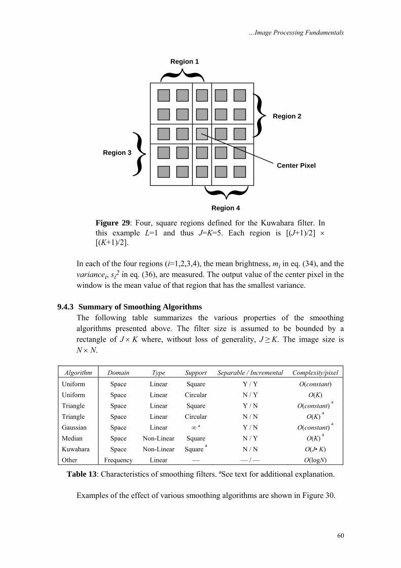
…Image Processing Fundamentals
60
Region 2}Region 1
Region 3}Region 4
Center Pixel
Figure 29: Four, square regions defined for the Kuwahara filter. In this example L=1 and thus J=K=5. Each region is [(J+1)/2] × [(K+1)/2].
In each of the four regions (i=1,2,3,4), the mean brightness, mi in eq. (34), and the variancei, si2 in eq. (36), are measured. The output value of the center pixel in the window is the mean value of that region that has the smallest variance.
9.4.3 Summary of Smoothing Algorithms The following table summarizes the various properties of the smoothing algorithms presented above. The filter size is assumed to be bounded by a rectangle of J × K where, without loss of generality, J ≥ K. The image size is N × N.
Algorithm Domain Type Support Separable / Incremental Complexity/pixel
Uniform Space Linear Square Y / Y O(constant) Uniform Space Linear Circular N / Y O(K) Triangle Space Linear Square Y / N O(constant) ª Triangle Space Linear Circular N / N O(K) ª Gaussian Space Linear ∞ ª Y / N O(constant) ª Median Space Non-Linear Square N / Y O(K) ª Kuwahara Space Non-Linear Square ª N / N O(J• K) Other Frequency Linear — — / — O(logN)
Table 13: Characteristics of smoothing filters. ªSee text for additional explanation. Examples of the effect of various smoothing algorithms are shown in Figure 30.
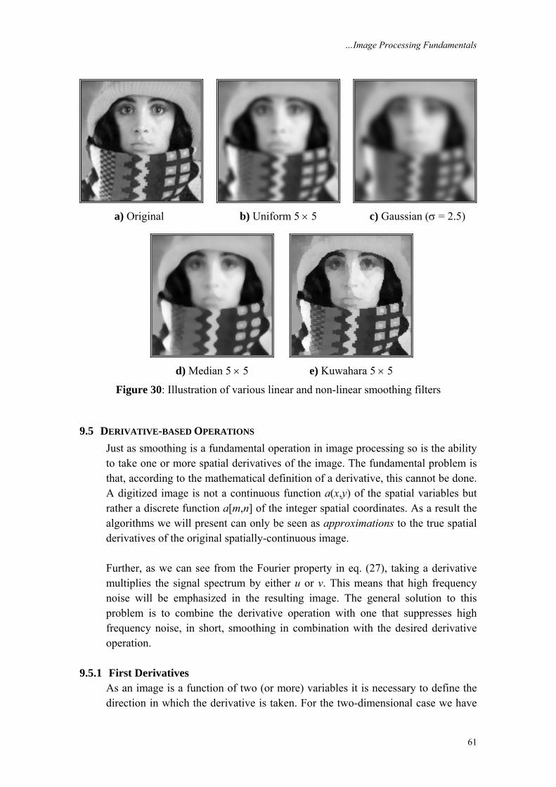
…Image Processing Fundamentals
61
a) Original b) Uniform 5 × 5 c) Gaussian (σ = 2.5)
d) Median 5 × 5 e) Kuwahara 5 × 5
Figure 30: Illustration of various linear and non-linear smoothing filters
9.5 DERIVATIVE-BASED OPERATIONS Just as smoothing is a fundamental operation in image processing so is the ability to take one or more spatial derivatives of the image. The fundamental problem is that, according to the mathematical definition of a derivative, this cannot be done. A digitized image is not a continuous function a(x,y) of the spatial variables but rather a discrete function a[m,n] of the integer spatial coordinates. As a result the algorithms we will present can only be seen as approximations to the true spatial derivatives of the original spatially-continuous image. Further, as we can see from the Fourier property in eq. (27), taking a derivative multiplies the signal spectrum by either u or v. This means that high frequency noise will be emphasized in the resulting image. The general solution to this problem is to combine the derivative operation with one that suppresses high frequency noise, in short, smoothing in combination with the desired derivative operation.
9.5.1 First Derivatives As an image is a function of two (or more) variables it is necessary to define the direction in which the derivative is taken. For the two-dimensional case we have
…Image Processing Fundamentals
62
the horizontal direction, the vertical direction, or an arbitrary direction which can be considered as a combination of the two. If we use hx to denote a horizontal derivative filter (matrix), hy to denote a vertical derivative filter (matrix), and hθ to denote the arbitrary angle derivative filter (matrix), then: [ ] [ ]cos • sin • yθ θ θ ⎡ ⎤= + ⎣ ⎦xh h h (102)
• Gradient filters – It is also possible to generate a vector derivative description as the gradient, ∇a[m,n], of an image:
( ) ( )x y x x y ya aa i i h a i h a ix y
∂ ∂∂ ∂
∇ = + = ⊗ + ⊗ (103)
where and x yi i are unit vectors in the horizontal and vertical direction, respectively. This leads to two descriptions:
Gradient magnitude – ( ) ( )22x ya h a h a∇ = ⊗ + ⊗ (104)
and
Gradient direction – ( ) ( )( )arctan y
x
h aa h aψ
⎧ ⎫⊗⎪ ⎪∇ = ⎨ ⎬⊗⎪ ⎪⎩ ⎭ (105)
The gradient magnitude is sometimes approximated by: Approx. Gradient magnitude – x ya h a h a∇ ≅ ⊗ + ⊗ (106)
The final results of these calculations depend strongly on the choices of hx and hy. A number of possible choices for (hx, hy) will now be described. • Basic derivative filters – These filters are specified by:
[ ] [ ]
[ ] [ ]
) 1 1
) 1 0 1
ty
ty
i
ii
⎡ ⎤= = −⎣ ⎦
⎡ ⎤= = −⎣ ⎦
x
x
h h
h h (107)
where “t” denotes matrix transpose. These two filters differ significantly in their Fourier magnitude and Fourier phase characteristics. For the frequency range 0 ≤ Ω ≤ π, these are given by:
…Image Processing Fundamentals
63
[ ] [ ] ( ) ( )
[ ] [ ]
) 1 1 ( ) 2 sin 2 ; ( ) 2
) 1 0 1 ( ) 2 sin ; ( ) / 2
i H
ii H
ϕ π
ϕ π
= − ↔ Ω = Ω Ω = − Ω
= − ↔ Ω = Ω Ω =
h
h
F
F (108)
The second form (ii) gives suppression of high frequency terms (Ω ≈ π) while the first form (i) does not. The first form leads to a phase shift; the second form does not. • Prewitt gradient filters – These filters are specified by:
[ ] [ ]
[ ]
1 0 1 11 11 0 1 1 • 1 0 13 3
1 0 1 1
1 1 1 11 10 0 0 0 • 1 1 13 3
1 1 1 1
x
y
−⎡ ⎤ ⎡ ⎤⎢ ⎥ ⎢ ⎥= − = −⎢ ⎥ ⎢ ⎥⎢ ⎥ ⎢ ⎥−⎣ ⎦ ⎣ ⎦
⎡ ⎤ ⎡ ⎤⎢ ⎥ ⎢ ⎥⎡ ⎤ = =⎣ ⎦ ⎢ ⎥ ⎢ ⎥⎢ ⎥ ⎢ ⎥− − − −⎣ ⎦ ⎣ ⎦
h
h
(109)
Both hx and hy are separable. Beyond the computational implications are the implications for the analysis of the filter. Each filter takes the derivative in one direction using eq. (107)ii and smoothes in the orthogonal direction using a one-dimensional version of a uniform filter as described in Section 9.4.1. • Sobel gradient filters – These filters are specified by:
[ ] [ ]
[ ]
1 0 1 11 12 0 2 2 • 1 0 14 4
1 0 1 1
1 2 1 11 10 0 0 0 • 1 2 14 4
1 2 1 1
x
y
−⎡ ⎤ ⎡ ⎤⎢ ⎥ ⎢ ⎥= − = −⎢ ⎥ ⎢ ⎥⎢ ⎥ ⎢ ⎥−⎣ ⎦ ⎣ ⎦
⎡ ⎤ ⎡ ⎤⎢ ⎥ ⎢ ⎥⎡ ⎤ = =⎣ ⎦ ⎢ ⎥ ⎢ ⎥⎢ ⎥ ⎢ ⎥− − − −⎣ ⎦ ⎣ ⎦
h
h
(110)
Again, hx and hy are separable. Each filter takes the derivative in one direction using eq. (107)ii and smoothes in the orthogonal direction using a one-dimensional version of a triangular filter as described in Section 9.4.1. • Alternative gradient filters – The variety of techniques available from one-dimensional signal processing for the design of digital filters offers us powerful tools for designing one-dimensional versions of hx and hy. Using the Parks-
…Image Processing Fundamentals
64
McClellan filter design algorithm, for example, we can choose the frequency bands where we want the derivative to be taken and the frequency bands where we want the noise to be suppressed. The algorithm will then produce a real, odd filter with a minimum length that meets the specifications. As an example, if we want a filter that has derivative characteristics in a passband (with weight 1.0) in the frequency range 0.0 ≤ Ω ≤ 0.3π and a stopband (with weight 3.0) in the range 0.32π ≤ Ω ≤ π, then the algorithm produces the following optimized seven sample filter:
[ ] [ ]13571 8212 15580 0 15580 8212 3571
16348x yt
= = − − −⎡ ⎤⎣ ⎦h h (111)
The gradient can then be calculated as in eq. (103). • Gaussian gradient filters – In modern digital image processing one of the most common techniques is to use a Gaussian filter (see Section 9.4.1) to accomplish the required smoothing and one of the derivatives listed in eq. (107). Thus, we might first apply the recursive Gaussian in eq. (97) followed by eq. (107)ii to achieve the desired, smoothed derivative filters hx and hy. Further, for computational efficiency, we can combine these two steps as:
( ) ( )
( )
1 2 3 0
1 2 3 0
[ ] [ 1] [ 1] [ 1] [ 2] [ 3] /2
[ ] [ ] [ 1] [ 2] [ 3] /
Bw n a n a n b w n b w n b w n b
c n Bw n b c n b c n b c n b
⎛ ⎞= + − − + − + − + −⎜ ⎟⎝ ⎠
= + + + + + + (112)
where the various coefficients are defined in eq. (99). The first (forward) equation is applied from n = 0 up to n = N – 1 while the second (backward) equation is applied from n = N – 1 down to n = 0. • Summary – Examples of the effect of various derivative algorithms on a noisy version of Figure 30a (SNR = 29 dB) are shown in Figure 31a-c. The effect of various magnitude gradient algorithms on Figure 30a are shown in Figure 32a-c. After processing, all images are contrast stretched as in eq. (77) for display purposes.
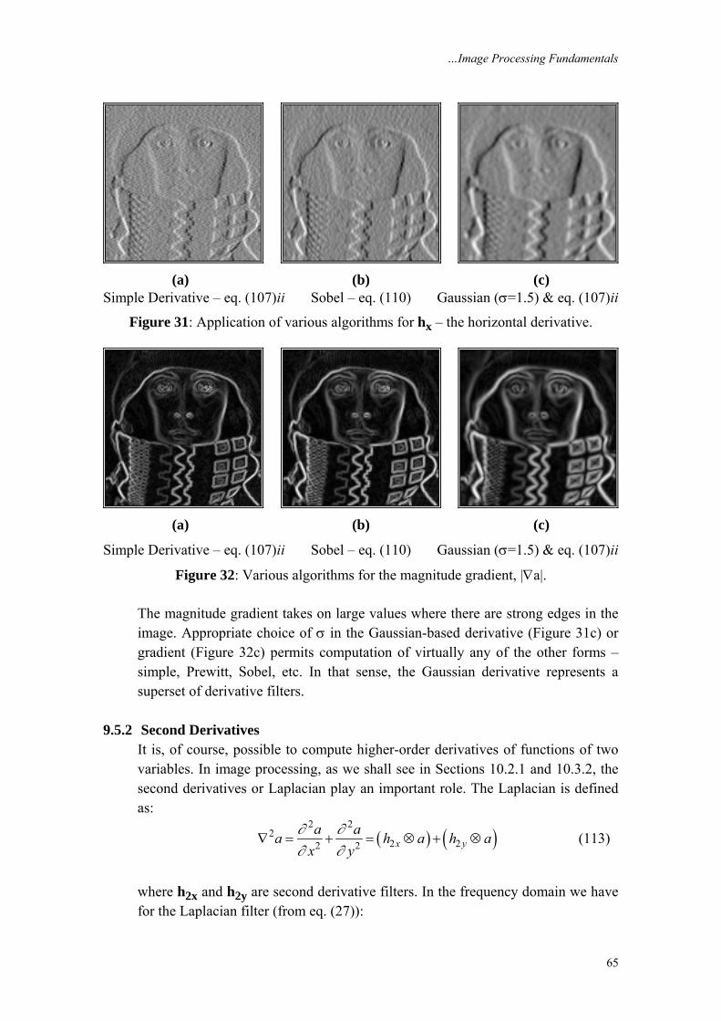
…Image Processing Fundamentals
65
(a) (b) (c) Simple Derivative – eq. (107)ii Sobel – eq. (110) Gaussian (σ=1.5) & eq. (107)ii
Figure 31: Application of various algorithms for hx – the horizontal derivative.
(a) (b) (c)
Simple Derivative – eq. (107)ii Sobel – eq. (110) Gaussian (σ=1.5) & eq. (107)ii
Figure 32: Various algorithms for the magnitude gradient, |∇a|. The magnitude gradient takes on large values where there are strong edges in the image. Appropriate choice of σ in the Gaussian-based derivative (Figure 31c) or gradient (Figure 32c) permits computation of virtually any of the other forms – simple, Prewitt, Sobel, etc. In that sense, the Gaussian derivative represents a superset of derivative filters.
9.5.2 Second Derivatives It is, of course, possible to compute higher-order derivatives of functions of two variables. In image processing, as we shall see in Sections 10.2.1 and 10.3.2, the second derivatives or Laplacian play an important role. The Laplacian is defined as:
( ) ( )2 2
22 22 2 x y
a aa h a h ax y
∂ ∂∂ ∂
∇ = + = ⊗ + ⊗ (113)
where h2x and h2y are second derivative filters. In the frequency domain we have for the Laplacian filter (from eq. (27)):
…Image Processing Fundamentals
66
( )2 2 2 ( , )a u v A u v∇ ↔ − +F
(114)
The transfer function of a Laplacian corresponds to a parabola H(u,v) = –(u2 + v2). • Basic second derivative filter – This filter is specified by:
[ ] [ ]2 2 1 2 1t
x y⎡ ⎤= = −⎣ ⎦h h (115)
and the frequency spectrum of this filter, in each direction, is given by: { } ( )( ) 1 2 1 2 1 cosFH Ω = − = − − Ω (116)
over the frequency range –π ≤ Ω ≤ π. The two, one-dimensional filters can be used in the manner suggested by eq. (113) or combined into one, two-dimensional filter as:
[ ]0 1 01 4 10 1 0
⎡ ⎤⎢ ⎥= −⎢ ⎥⎢ ⎥⎣ ⎦
h (117)
and used as in eq. (84). • Frequency domain Laplacian – This filter is the implementation of the general recipe given in eq. (92) and for the Laplacian filter takes the form: ( ) ( ){ }1 2 2[ , ] ,c m n A−= − Ω + Ψ Ω ΨF (118)
• Gaussian second derivative filter – This is the straightforward extension of the Gaussian first derivative filter described above and can be applied independently in each dimension. We first apply Gaussian smoothing with a σ chosen on the basis of the problem specification. We then apply the desired second derivative filter eq. (115) or eq. (118). Again there is the choice among the various Gaussian smoothing algorithms. For efficiency, we can use the recursive implementation and combine the two steps—smoothing and derivative operation—as follows:
( ) ( )( ) ( )
1 2 3 0
1 2 3 0
[ ] [ ] [ 1] [ 1] [ 2] [ 3] /
[ ] [ 1] [ ] [ 1] [ 2] [ 3] /
w n B a n a n b w n b w n b w n b
c n B w n w n b c n b c n b c n b
= − − + − + − + −
= + − + + + + + + (119)
…Image Processing Fundamentals
67
where the various coefficients are defined in eq. (99). Again, the first (forward) equation is applied from n = 0 up to n = N – 1 while the second (backward) equation is applied from n = N – 1 down to n = 0. • Alternative Laplacian filters – Again one-dimensional digital filter design techniques offer us powerful methods to create filters that are optimized for a specific problem. Using the Parks-McClellan design algorithm, we can choose the frequency bands where we want the second derivative to be taken and the frequency bands where we want the noise to be suppressed. The algorithm will then produce a real, even filter with a minimum length that meets the specifications. As an example, if we want a filter that has second derivative characteristics in a passband (with weight 1.0) in the frequency range 0.0 ≤ Ω ≤ 0.3π and a stopband (with weight 3.0) in the range 0.32π ≤ Ω ≤ π, then the algorithm produces the following optimized seven sample filter:
[ ] [ ]13448 10145 1495 16383 1495 10145 3448
11043x yt
= = − − −⎡ ⎤⎣ ⎦h h (120)
The Laplacian can then be calculated as in eq. (113). • SDGD filter – A filter that is especially useful in edge finding and object measurement is the Second-Derivative-in-the-Gradient-Direction (SDGD) filter. This filter uses five partial derivatives:
2 2
2
2 2
2
xx xy x
yx yy y
a a aA A Ax y xx
a a aA A Ax y yy
∂ ∂ ∂∂ ∂ ∂∂
∂ ∂ ∂∂ ∂ ∂∂
= = =
= = =
(121)
Note that Axy = Ayx which accounts for the five derivatives. This SDGD combines the different partial derivatives as follows:
2 2
2 2
2( ) xx x xy x y yy y
x y
A A A A A A ASDGD a
A A+ +
=+
(122)
As one might expect, the large number of derivatives involved in this filter implies that noise suppression is important and that Gaussian derivative filters—
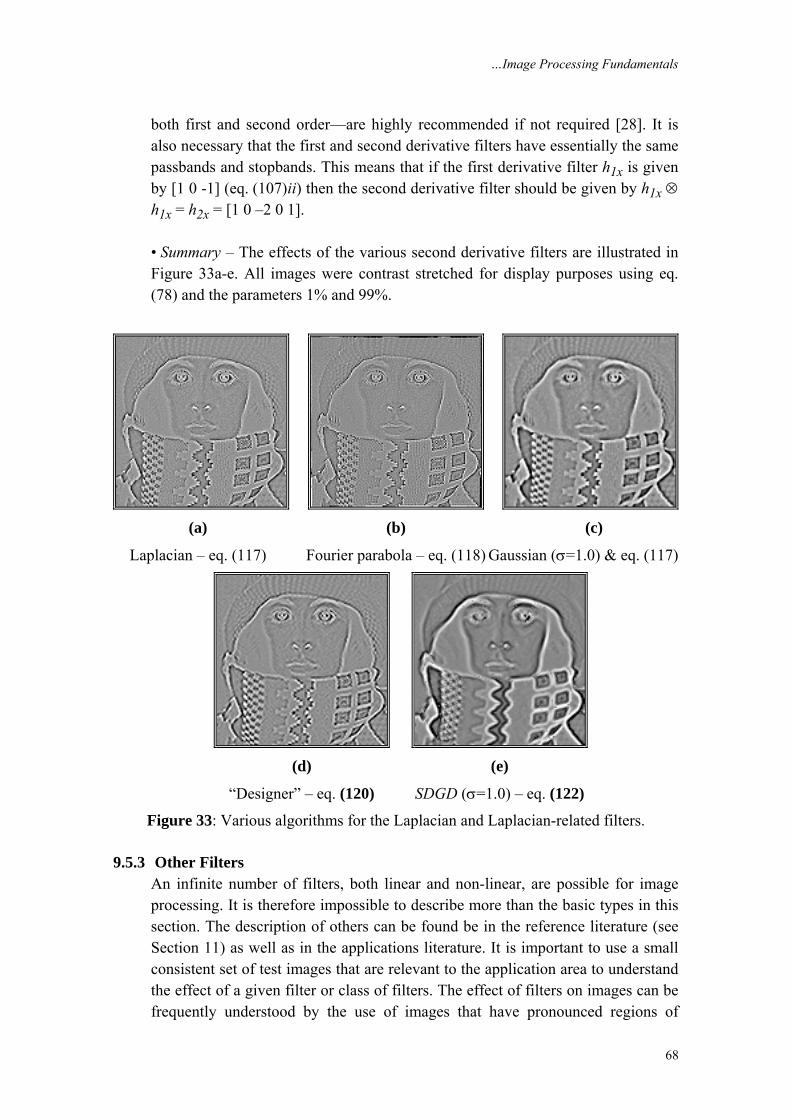
…Image Processing Fundamentals
68
both first and second order—are highly recommended if not required [28]. It is also necessary that the first and second derivative filters have essentially the same passbands and stopbands. This means that if the first derivative filter h1x is given by [1 0 -1] (eq. (107)ii) then the second derivative filter should be given by h1x ⊗ h1x = h2x = [1 0 –2 0 1]. • Summary – The effects of the various second derivative filters are illustrated in Figure 33a-e. All images were contrast stretched for display purposes using eq. (78) and the parameters 1% and 99%.
(a) (b) (c)
Laplacian – eq. (117) Fourier parabola – eq. (118) Gaussian (σ=1.0) & eq. (117)
(d) (e)
“Designer” – eq. (120) SDGD (σ=1.0) – eq. (122)
Figure 33: Various algorithms for the Laplacian and Laplacian-related filters.
9.5.3 Other Filters An infinite number of filters, both linear and non-linear, are possible for image processing. It is therefore impossible to describe more than the basic types in this section. The description of others can be found be in the reference literature (see Section 11) as well as in the applications literature. It is important to use a small consistent set of test images that are relevant to the application area to understand the effect of a given filter or class of filters. The effect of filters on images can be frequently understood by the use of images that have pronounced regions of
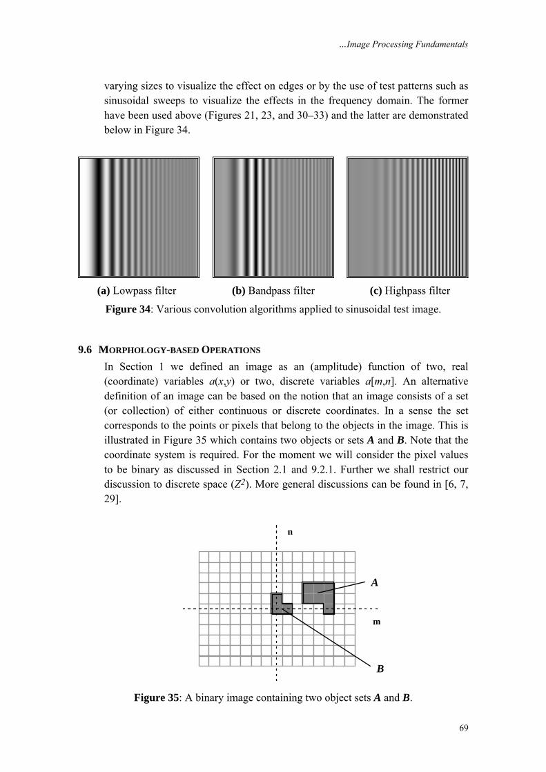
…Image Processing Fundamentals
69
varying sizes to visualize the effect on edges or by the use of test patterns such as sinusoidal sweeps to visualize the effects in the frequency domain. The former have been used above (Figures 21, 23, and 30–33) and the latter are demonstrated below in Figure 34.
(a) Lowpass filter (b) Bandpass filter (c) Highpass filter
Figure 34: Various convolution algorithms applied to sinusoidal test image.
9.6 MORPHOLOGY-BASED OPERATIONS In Section 1 we defined an image as an (amplitude) function of two, real (coordinate) variables a(x,y) or two, discrete variables a[m,n]. An alternative definition of an image can be based on the notion that an image consists of a set (or collection) of either continuous or discrete coordinates. In a sense the set corresponds to the points or pixels that belong to the objects in the image. This is illustrated in Figure 35 which contains two objects or sets A and B. Note that the coordinate system is required. For the moment we will consider the pixel values to be binary as discussed in Section 2.1 and 9.2.1. Further we shall restrict our discussion to discrete space (Z2). More general discussions can be found in [6, 7, 29].
n
m
A
B
Figure 35: A binary image containing two object sets A and B.
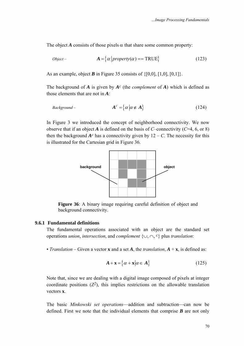
…Image Processing Fundamentals
70
The object A consists of those pixels α that share some common property: Object – { }( ) TRUEpropertyα α= ==A (123)
As an example, object B in Figure 35 consists of {[0,0], [1,0], [0,1]}. The background of A is given by Ac (the complement of A) which is defined as those elements that are not in A: Background – { }c α α= ∉A A (124)
In Figure 3 we introduced the concept of neighborhood connectivity. We now observe that if an object A is defined on the basis of C–connectivity (C=4, 6, or 8) then the background Ac has a connectivity given by 12 – C. The necessity for this is illustrated for the Cartesian grid in Figure 36.
background object
Figure 36: A binary image requiring careful definition of object and background connectivity.
9.6.1 Fundamental definitions The fundamental operations associated with an object are the standard set operations union, intersection, and complement {∪, ∩, c} plus translation: • Translation – Given a vector x and a set A, the translation, A + x, is defined as: { }α α+ = + ∈x xA A (125)
Note that, since we are dealing with a digital image composed of pixels at integer coordinate positions (Z2), this implies restrictions on the allowable translation vectors x. The basic Minkowski set operations—addition and subtraction—can now be defined. First we note that the individual elements that comprise B are not only
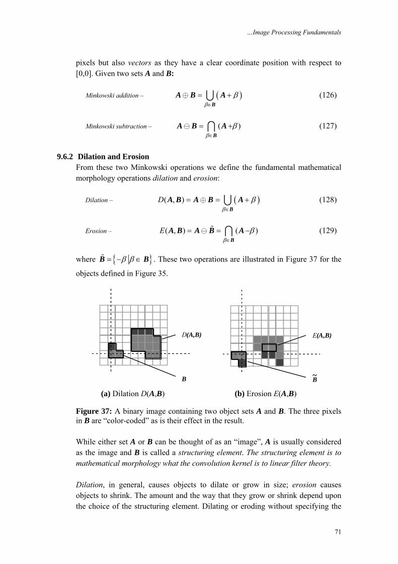
…Image Processing Fundamentals
71
pixels but also vectors as they have a clear coordinate position with respect to [0,0]. Given two sets A and B: Minkowski addition – ( )
ββ
∈
= +∪⊕B
A B A (126)
Minkowski subtraction – ( )
ββ
∈
= +∩B
A B A (127)
9.6.2 Dilation and Erosion From these two Minkowski operations we define the fundamental mathematical morphology operations dilation and erosion: Dilation – ( )( , )D
ββ
∈
= = +∪⊕B
A B A B A (128)
Erosion – ( , ) ( )E
ββ
∈
= = −∩B
A B A B A (129)
where { }β β= − ∈B B . These two operations are illustrated in Figure 37 for the
objects defined in Figure 35.
(a) Dilation D(A,B) (b) Erosion E(A,B)
Figure 37: A binary image containing two object sets A and B. The three pixels in B are “color-coded” as is their effect in the result. While either set A or B can be thought of as an “image”, A is usually considered as the image and B is called a structuring element. The structuring element is to mathematical morphology what the convolution kernel is to linear filter theory. Dilation, in general, causes objects to dilate or grow in size; erosion causes objects to shrink. The amount and the way that they grow or shrink depend upon the choice of the structuring element. Dilating or eroding without specifying the
B
E(A,B)
~B
D(A,B)
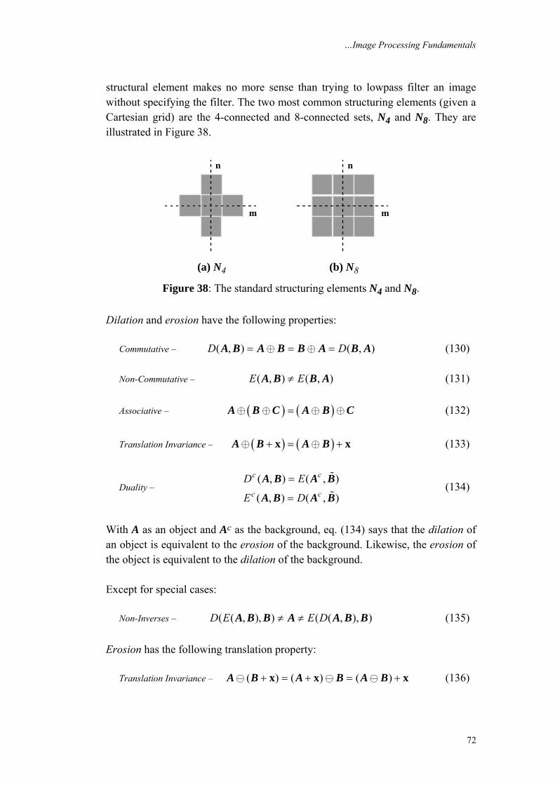
…Image Processing Fundamentals
72
structural element makes no more sense than trying to lowpass filter an image without specifying the filter. The two most common structuring elements (given a Cartesian grid) are the 4-connected and 8-connected sets, N4 and N8. They are illustrated in Figure 38.
n
m
n
m
(a) N4 (b) N8
Figure 38: The standard structuring elements N4 and N8. Dilation and erosion have the following properties: Commutative – ( , ) ( , )D D= = =⊕ ⊕A B A B B A B A (130) Non-Commutative – ( , ) ( , )E E≠A B B A (131) Associative – ( ) ( )=⊕ ⊕ ⊕ ⊕A B C A B C (132)
Translation Invariance – ( ) ( )+ = +x x⊕ ⊕A B A B (133)
Duality – ( , ) ( , )
( , ) ( , )
c c
c c
D E
E D
=
=
A B A B
A B A B (134)
With A as an object and Ac as the background, eq. (134) says that the dilation of an object is equivalent to the erosion of the background. Likewise, the erosion of the object is equivalent to the dilation of the background. Except for special cases: Non-Inverses – ( ( , ), ) ( ( , ), )D E E D≠ ≠A B B A A B B (135) Erosion has the following translation property: Translation Invariance – ( ) ( ) ( )+ = + = +x x xA B A B A B (136)
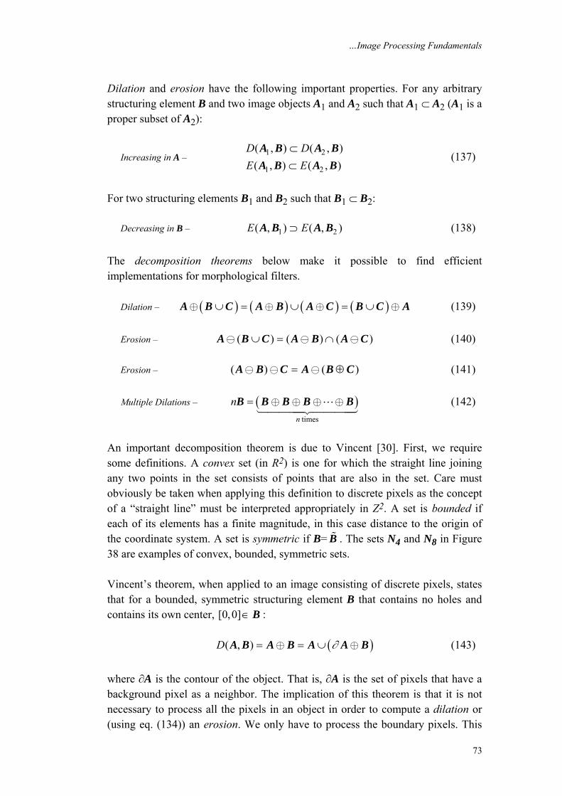
…Image Processing Fundamentals
73
Dilation and erosion have the following important properties. For any arbitrary structuring element B and two image objects A1 and A2 such that A1 ⊂ A2 (A1 is a proper subset of A2):
Increasing in A – 1 2
1 2
( , ) ( , )( , ) ( , )
D DE E
⊂⊂
A B A BA B A B
(137)
For two structuring elements B1 and B2 such that B1 ⊂ B2: Decreasing in B – 1 2( , ) ( , )E E⊃A B A B (138) The decomposition theorems below make it possible to find efficient implementations for morphological filters. Dilation – ( ) ( ) ( ) ( )∪ = ∪ = ∪⊕ ⊕ ⊕ ⊕A B C A B A C B C A (139)
Erosion – ( ) ( ) ( )∪ = ∩A B C A B A C (140) Erosion – ( ) ( )= ⊕A B C A B C (141) Multiple Dilations – ( )
timesn
n = ⊕ ⊕ ⊕ ⊕B B B B B (142)
An important decomposition theorem is due to Vincent [30]. First, we require some definitions. A convex set (in R2) is one for which the straight line joining any two points in the set consists of points that are also in the set. Care must obviously be taken when applying this definition to discrete pixels as the concept of a “straight line” must be interpreted appropriately in Z2. A set is bounded if each of its elements has a finite magnitude, in this case distance to the origin of the coordinate system. A set is symmetric if B= B . The sets N4 and N8 in Figure 38 are examples of convex, bounded, symmetric sets. Vincent’s theorem, when applied to an image consisting of discrete pixels, states that for a bounded, symmetric structuring element B that contains no holes and contains its own center, [0,0]∈ B : ( )( , )D ∂= = ∪⊕ ⊕A B A B A A B (143)
where ∂A is the contour of the object. That is, ∂A is the set of pixels that have a background pixel as a neighbor. The implication of this theorem is that it is not necessary to process all the pixels in an object in order to compute a dilation or (using eq. (134)) an erosion. We only have to process the boundary pixels. This
…Image Processing Fundamentals
74
also holds for all operations that can be derived from dilations and erosions. The processing of boundary pixels instead of object pixels means that, except for pathological images, computational complexity can be reduced from O(N2) to O(N) for an N × N image. A number of “fast” algorithms can be found in the literature that are based on this result [30-32]. The simplest dilation and erosion algorithms are frequently described as follows. • Dilation – Take each binary object pixel (with value “1”) and set all background pixels (with value “0”) that are C-connected to that object pixel to the value “1”. • Erosion – Take each binary object pixel (with value “1”) that is C-connected to a background pixel and set the object pixel value to “0”. Comparison of these two procedures to eq. (143) where B = NC=4 or NC=8 shows that they are equivalent to the formal definitions for dilation and erosion. The procedure is illustrated for dilation in Figure 39.
(a) B = N4 (b) B= N8
Figure 39: Illustration of dilation. Original object pixels are in gray; pixels added through dilation are in black.
9.6.3 Boolean Convolution An arbitrary binary image object (or structuring element) A can be represented as:
[ , ] • [ , ]k j
a j k m j n kδ+∞ +∞
=−∞ =−∞↔ − −∑ ∑A (144)
where Σ and • are the Boolean operations OR and AND as defined in eqs. (81) and (82), a[j,k] is a characteristic function that takes on the Boolean values “1” and “0” as follows:
1
[ , ]0
aa j k
a∈⎧
= ⎨ ∉⎩
AA
(145)
…Image Processing Fundamentals
75
and δ[m,n] is a Boolean version of the Dirac delta function that takes on the Boolean values “1” and “0” as follows:
1 0
[ , ]0
j kj k
otherwiseδ
= =⎧= ⎨
⎩ (146)
Dilation for binary images can therefore be written as:
( , ) [ , ] • [ , ]k j
D a j k b m j n k+∞ +∞
=−∞ =−∞= − − = ⊗∑ ∑A B a b (147)
which, because Boolean OR and AND are commutative, can also be written as
( , ) [ , ] • [ , ] ( , )k j
D a m j n k b j k D+∞ +∞
=−∞ =−∞= − − = ⊗ =∑ ∑A B b a B A (148)
Using De Morgan’s theorem: ( ) ( )• and •a b a b a b a b+ = = + (149)
on eq. (148) together with eq. (134), erosion can be written as:
( )( , ) [ , ] [ , ]k j
E a m j n k b j k+∞ +∞
=−∞ =−∞
= − − + − −∏ ∏A B (150)
Thus, dilation and erosion on binary images can be viewed as a form of convolution over a Boolean algebra. In Section 9.3.2 we saw that, when convolution is employed, an appropriate choice of the boundary conditions for an image is essential. Dilation and erosion—being a Boolean convolution—are no exception. The two most common choices are that either everything outside the binary image is “0” or everything outside the binary image is “1”.
9.6.4 Opening and Closing We can combine dilation and erosion to build two important higher order operations: Opening – ( , ) ( ( , ), )O D E= =A B A B A B B (151) Closing – ( , ) ( ( , ), )C E D= =•A B A B A B B (152)
…Image Processing Fundamentals
76
The opening and closing have the following properties:
Duality – ( , ) ( , )
( , ) ( , )
c c
c c
C O
O C
=
=
A B A B
A B A B (153)
Translation – ( , ) ( , )( , ) ( , )
O OC C
+ = ++ = +
x xx x
A B A BA B A B
(154)
For the opening with structuring element B and images A, A1, and A2, where A1 is a subimage of A2 (A1 ⊆ A2): Antiextensivity – ( , )O ⊆A B A (155) Increasing monotonicity – 1 2( , ) ( , )O O⊆A B A B (156) Idempotence – ( ( , ), ) ( , )O O O=A B B A B (157) For the closing with structuring element B and images A, A1, and A2, where A1 is a subimage of A2 (A1 ⊆ A2): Extensivity – ( , )C⊆A A B (158) Increasing monotonicity – 1 2( , ) ( , )C C⊆A B A B (159) Idempotence – ( ( , ), ) ( , )C C C=A B B A B (160) The two properties given by eqs. (155) and (84) are so important to mathematical morphology that they can be considered as the reason for defining erosion with B instead of B in eq. (129).
9.6.5 Hit–and–Miss operation The hit-or-miss operator was defined by Serra but we shall refer to it as the hit-and-miss operator and define it as follows. Given an image A and two structuring elements B1 and B2, the set definition and Boolean definition are:
Hit-and-Miss –
( ) ( )
( ) ( )
1 2
1 2
1 2
, ,
( , , )
, • ,
cE E
HitMiss
E E
⎧ ∩⎪⎪= ⎨⎪⎪⎩
A B A B
A B B
A B A B
(161)
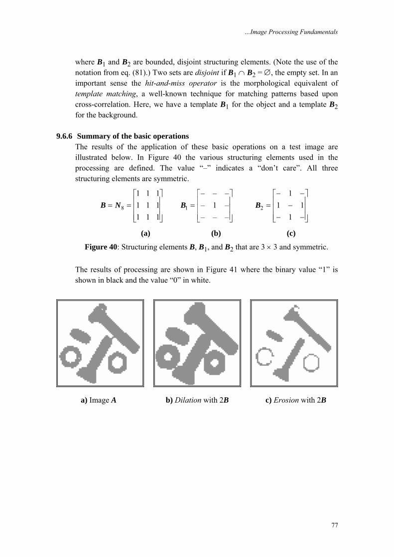
…Image Processing Fundamentals
77
where B1 and B2 are bounded, disjoint structuring elements. (Note the use of the notation from eq. (81).) Two sets are disjoint if B1 ∩ B2 = ∅, the empty set. In an important sense the hit-and-miss operator is the morphological equivalent of template matching, a well-known technique for matching patterns based upon cross-correlation. Here, we have a template B1 for the object and a template B2 for the background.
9.6.6 Summary of the basic operations The results of the application of these basic operations on a test image are illustrated below. In Figure 40 the various structuring elements used in the processing are defined. The value “–” indicates a “don’t care”. All three structuring elements are symmetric.
8
1 1 11 1 11 1 1
⎡ ⎤⎢ ⎥= = ⎢ ⎥⎢ ⎥⎣ ⎦
B N 1
– – –– 1 –– – –
⎡ ⎤⎢ ⎥= ⎢ ⎥⎢ ⎥⎣ ⎦
B 2
11 1
1
− −⎡ ⎤⎢ ⎥= −⎢ ⎥⎢ ⎥− −⎣ ⎦
B
(a) (b) (c)
Figure 40: Structuring elements B, B1, and B2 that are 3 × 3 and symmetric. The results of processing are shown in Figure 41 where the binary value “1” is shown in black and the value “0” in white.
a) Image A b) Dilation with 2B c) Erosion with 2B
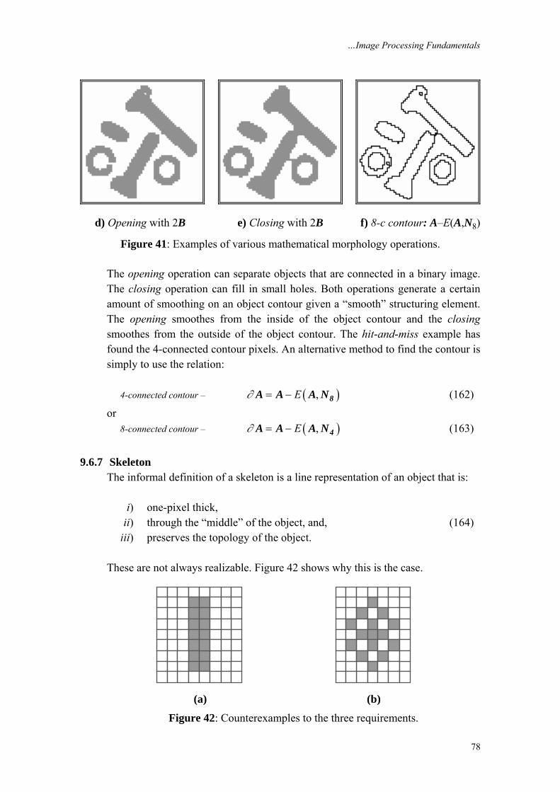
…Image Processing Fundamentals
78
d) Opening with 2B e) Closing with 2B f) 8-c contour: A–E(A,N8)
Figure 41: Examples of various mathematical morphology operations. The opening operation can separate objects that are connected in a binary image. The closing operation can fill in small holes. Both operations generate a certain amount of smoothing on an object contour given a “smooth” structuring element. The opening smoothes from the inside of the object contour and the closing smoothes from the outside of the object contour. The hit-and-miss example has found the 4-connected contour pixels. An alternative method to find the contour is simply to use the relation: 4-connected contour – ( ),E∂ = − 8A A A N (162)
or 8-connected contour – ( ),E∂ = − 4A A A N (163)
9.6.7 Skeleton The informal definition of a skeleton is a line representation of an object that is: i) one-pixel thick, ii) through the “middle” of the object, and, (164) iii) preserves the topology of the object. These are not always realizable. Figure 42 shows why this is the case.
(a) (b)
Figure 42: Counterexamples to the three requirements.
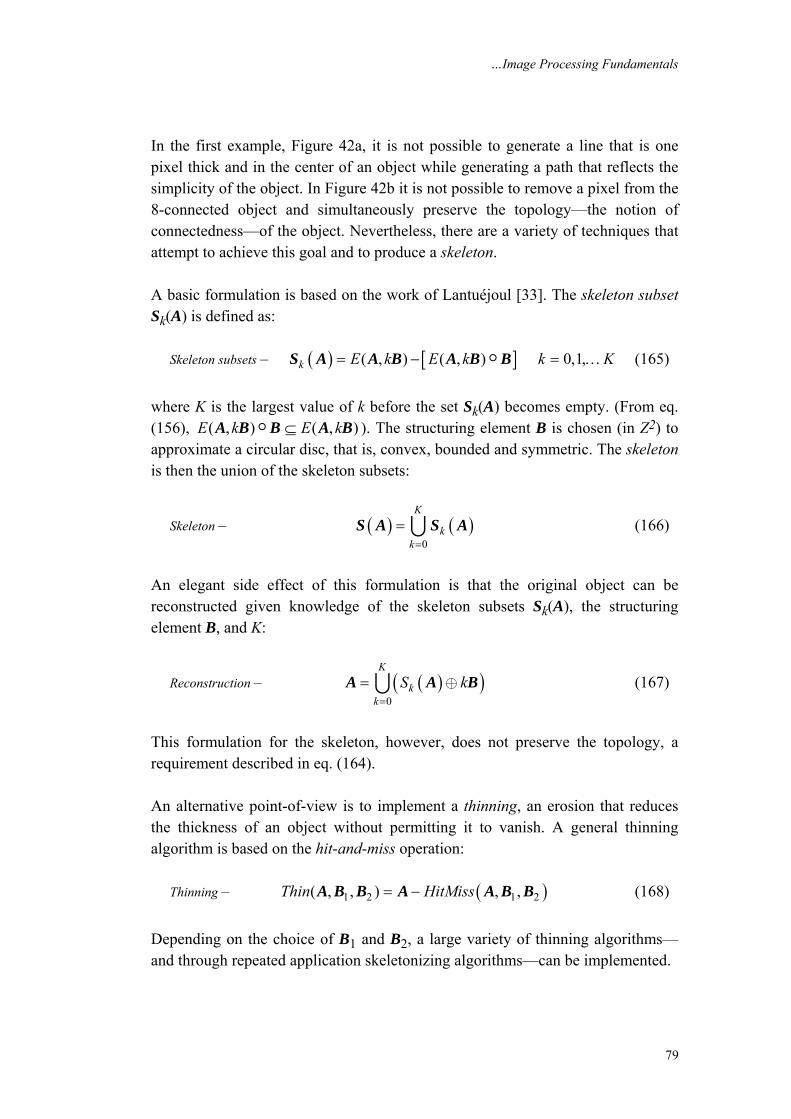
…Image Processing Fundamentals
79
In the first example, Figure 42a, it is not possible to generate a line that is one pixel thick and in the center of an object while generating a path that reflects the simplicity of the object. In Figure 42b it is not possible to remove a pixel from the 8-connected object and simultaneously preserve the topology—the notion of connectedness—of the object. Nevertheless, there are a variety of techniques that attempt to achieve this goal and to produce a skeleton. A basic formulation is based on the work of Lantuéjoul [33]. The skeleton subset Sk(A) is defined as: Skeleton subsets – ( ) [ ]( , ) ( , ) 0,1,k E k E k k K= − = …S A A B A B B (165)
where K is the largest value of k before the set Sk(A) becomes empty. (From eq. (156), ( , ) ( , )E k E k⊆A B B A B ). The structuring element B is chosen (in Z2) to approximate a circular disc, that is, convex, bounded and symmetric. The skeleton is then the union of the skeleton subsets:
Skeleton – ( ) ( )0
K
kk=
= ∪S A S A (166)
An elegant side effect of this formulation is that the original object can be reconstructed given knowledge of the skeleton subsets Sk(A), the structuring element B, and K:
Reconstruction – ( )( )0
K
kk
S k=
= ∪ ⊕A A B (167)
This formulation for the skeleton, however, does not preserve the topology, a requirement described in eq. (164). An alternative point-of-view is to implement a thinning, an erosion that reduces the thickness of an object without permitting it to vanish. A general thinning algorithm is based on the hit-and-miss operation: Thinning – ( )1 2 1 2( , , ) , ,Thin HitMiss= −A B B A A B B (168)
Depending on the choice of B1 and B2, a large variety of thinning algorithms—and through repeated application skeletonizing algorithms—can be implemented.
…Image Processing Fundamentals
80
A quite practical implementation can be described in another way. If we restrict ourselves to a 3 × 3 neighborhood, similar to the structuring element B = N8 in Figure 40a, then we can view the thinning operation as a window that repeatedly scans over the (binary) image and sets the center pixel to “0” under certain conditions. The center pixel is not changed to “0” if and only if: i) an isolated pixel is found (e.g. Figure 43a), ii) removing a pixel would change the connectivity (e.g. Figure 43b), (169) iii) removing a pixel would shorten a line (e.g. Figure 43c). As pixels are (potentially) removed in each iteration, the process is called a conditional erosion. Three test cases of eq. (169) are illustrated in Figure 43. In general all possible rotations and variations have to be checked. As there are only 512 possible combinations for a 3 × 3 window on a binary image, this can be done easily with the use of a lookup table.
(a) Isolated pixel (b) Connectivity pixel (c) End pixel
Figure 43: Test conditions for conditional erosion of the center pixel. If only condition (i) is used then each object will be reduced to a single pixel. This is useful if we wish to count the number of objects in an image. If only condition (ii) is used then holes in the objects will be found. If conditions (i + ii) are used each object will be reduced to either a single pixel if it does not contain a hole or to closed rings if it does contain holes. If conditions (i + ii + iii) are used then the “complete skeleton” will be generated as an approximation to eq. (56). Illustrations of these various possibilities are given in Figure 44a,b.
9.6.8 Propagation It is convenient to be able to reconstruct an image that has “survived” several erosions or to fill an object that is defined, for example, by a boundary. The formal mechanism for this has several names including region-filling, reconstruction, and propagation. The formal definition is given by the following algorithm. We start with a seed image S(0), a mask image A, and a structuring element B. We then use dilations of S with structuring element B and masked by A in an iterative procedure as follows: Iteration k – ( ) ( 1) ( ) ( 1)untilk k k k− −⎡ ⎤= ∩ =⎣ ⎦⊕S S B A S S (170)
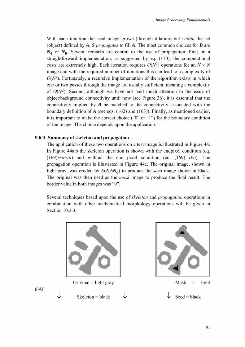
…Image Processing Fundamentals
81
With each iteration the seed image grows (through dilation) but within the set (object) defined by A; S propagates to fill A. The most common choices for B are N4 or N8. Several remarks are central to the use of propagation. First, in a straightforward implementation, as suggested by eq. (170), the computational costs are extremely high. Each iteration requires O(N2) operations for an N × N image and with the required number of iterations this can lead to a complexity of O(N3). Fortunately, a recursive implementation of the algorithm exists in which one or two passes through the image are usually sufficient, meaning a complexity of O(N2). Second, although we have not paid much attention to the issue of object/background connectivity until now (see Figure 36), it is essential that the connectivity implied by B be matched to the connectivity associated with the boundary definition of A (see eqs. (162) and (163)). Finally, as mentioned earlier, it is important to make the correct choice (“0” or “1”) for the boundary condition of the image. The choice depends upon the application.
9.6.9 Summary of skeleton and propagation The application of these two operations on a test image is illustrated in Figure 44. In Figure 44a,b the skeleton operation is shown with the endpixel condition (eq. (169)i+ii+iii) and without the end pixel condition (eq. (169) i+ii). The propagation operation is illustrated in Figure 44c. The original image, shown in light gray, was eroded by E(A,6N8) to produce the seed image shown in black. The original was then used as the mask image to produce the final result. The border value in both images was “0”. Several techniques based upon the use of skeleton and propagation operations in combination with other mathematical morphology operations will be given in Section 10.3.3.
Original = light gray Mask = light gray
↓ Skeleton = black ↓ ↓ Seed = black
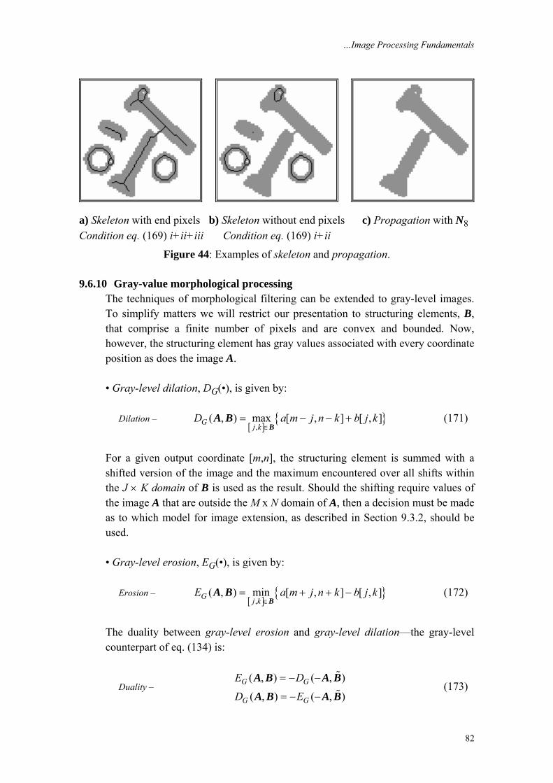
…Image Processing Fundamentals
82
a) Skeleton with end pixels b) Skeleton without end pixels c) Propagation with N8 Condition eq. (169) i+ii+iii Condition eq. (169) i+ii
Figure 44: Examples of skeleton and propagation.
9.6.10 Gray-value morphological processing The techniques of morphological filtering can be extended to gray-level images. To simplify matters we will restrict our presentation to structuring elements, B, that comprise a finite number of pixels and are convex and bounded. Now, however, the structuring element has gray values associated with every coordinate position as does the image A. • Gray-level dilation, DG(•), is given by: Dilation –
[ ]{ }
,( , ) max [ , ] [ , ]G j k
D a m j n k b j k∈
= − − +B
A B (171)
For a given output coordinate [m,n], the structuring element is summed with a shifted version of the image and the maximum encountered over all shifts within the J × K domain of B is used as the result. Should the shifting require values of the image A that are outside the M x N domain of A, then a decision must be made as to which model for image extension, as described in Section 9.3.2, should be used. • Gray-level erosion, EG(•), is given by: Erosion –
[ ]{ }
,( , ) min [ , ] [ , ]G j k
E a m j n k b j k∈
= + + −B
A B (172)
The duality between gray-level erosion and gray-level dilation—the gray-level counterpart of eq. (134) is:
Duality – ( , ) ( , )
( , ) ( , )G G
G G
E D
D E
= − −
= − −
A B A B
A B A B (173)
…Image Processing Fundamentals
83
where “ A ” means that a[j,k] → a[–j,–k] and “ −A” means that a[j,k] → –a[j,k]. The definitions of higher order operations such as gray-level opening and gray-level closing are: Opening – ( , ) ( ( , ), )G G GO D E=A B A B B (174) Closing – ( )( )( , ) , ,G G GC E D=A B A B B (175)
The duality between gray-level opening and gray-level closing is:
Duality – ( , ) ( , )( , ) ( , )
G G
G G
O CC O
= − −
= − −
A B A BA B A B
(176)
The important properties that were discussed earlier such as idempotence, translation invariance, increasing in A, and so forth are also applicable to gray level morphological processing. The details can be found in Giardina and Dougherty [6]. In many situations the seeming complexity of gray level morphological processing is significantly reduced through the use of symmetric structuring elements where b[j,k] = b[–j,–k]. The most common of these is based on the use of B = constant = 0. For this important case and using again the domain [j,k] ∈ B, the definitions above reduce to: Dilation –
[ ]{ } ( )
,( , ) max [ , ] maxG j k
D a m j n k∈
= − − =B B
A B A (177)
Erosion –
[ ]{ } ( )
,( , ) min [ , ] minG j k
E a m j n k∈
= + + =B B
A B A (178)
Opening – ( , ) max(min( ))GO =
BBA B A (179)
Closing – ( , ) min(max( ))GC =
B BA B A (180)
The remarkable conclusion is that the maximum filter and the minimum filter, introduced in Section 9.4.2, are gray-level dilation and gray-level erosion for the specific structuring element given by the shape of the filter window with the gray value “0” inside the window. Examples of these operations on a simple one-dimensional signal are shown in Figure 45.
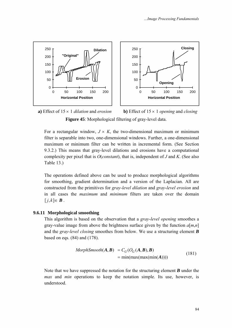
…Image Processing Fundamentals
84
0
50
100
150
200
250
0 50 100 150 200
Horizontal Position
Dilation
Erosion
"Original"
0
50
100
150
200
250
0 50 100 150 200
Horizontal Position
Closing
Opening
a) Effect of 15 × 1 dilation and erosion b) Effect of 15 × 1 opening and closing
Figure 45: Morphological filtering of gray-level data. For a rectangular window, J × K, the two-dimensional maximum or minimum filter is separable into two, one-dimensional windows. Further, a one-dimensional maximum or minimum filter can be written in incremental form. (See Section 9.3.2.) This means that gray-level dilations and erosions have a computational complexity per pixel that is O(constant), that is, independent of J and K. (See also Table 13.) The operations defined above can be used to produce morphological algorithms for smoothing, gradient determination and a version of the Laplacian. All are constructed from the primitives for gray-level dilation and gray-level erosion and in all cases the maximum and minimum filters are taken over the domain [ , ]j k ∈ B .
9.6.11 Morphological smoothing This algorithm is based on the observation that a gray-level opening smoothes a gray-value image from above the brightness surface given by the function a[m,n] and the gray-level closing smoothes from below. We use a structuring element B based on eqs. (84) and (178).
( , ) ( ( , ), )
min(max(max(min( ))))G GMorphSmooth C O=
=
A B A B BA
(181)
Note that we have suppressed the notation for the structuring element B under the max and min operations to keep the notation simple. Its use, however, is understood.
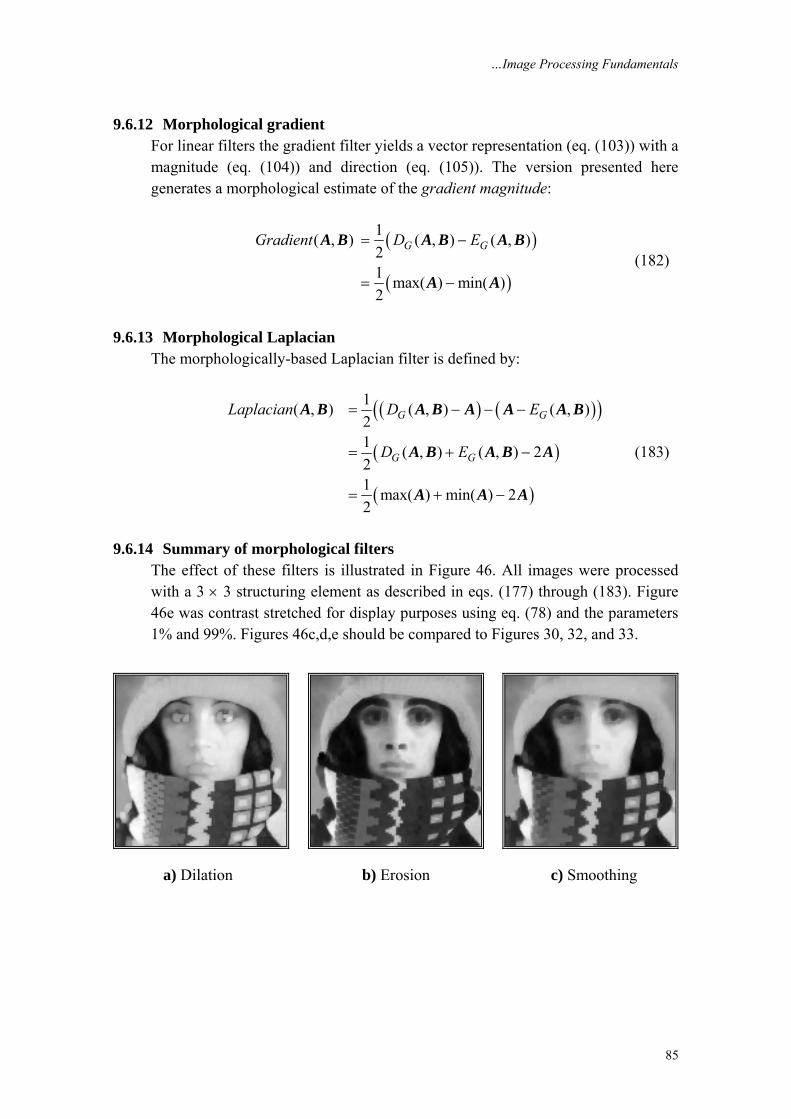
…Image Processing Fundamentals
85
9.6.12 Morphological gradient For linear filters the gradient filter yields a vector representation (eq. (103)) with a magnitude (eq. (104)) and direction (eq. (105)). The version presented here generates a morphological estimate of the gradient magnitude:
( )
( )
1( , ) ( , ) ( , )21 max( ) min( )2
G GGradient D E= −
= −
A B A B A B
A A (182)
9.6.13 Morphological Laplacian The morphologically-based Laplacian filter is defined by:
( ) ( )( )
( )
( )
1( , ) ( , ) ( , )21 ( , ) ( , ) 221 max( ) min( ) 22
G G
G G
Laplacian D E
D E
= − − −
= + −
= + −
A B A B A A A B
A B A B A
A A A
(183)
9.6.14 Summary of morphological filters The effect of these filters is illustrated in Figure 46. All images were processed with a 3 × 3 structuring element as described in eqs. (177) through (183). Figure 46e was contrast stretched for display purposes using eq. (78) and the parameters 1% and 99%. Figures 46c,d,e should be compared to Figures 30, 32, and 33.
a) Dilation b) Erosion c) Smoothing
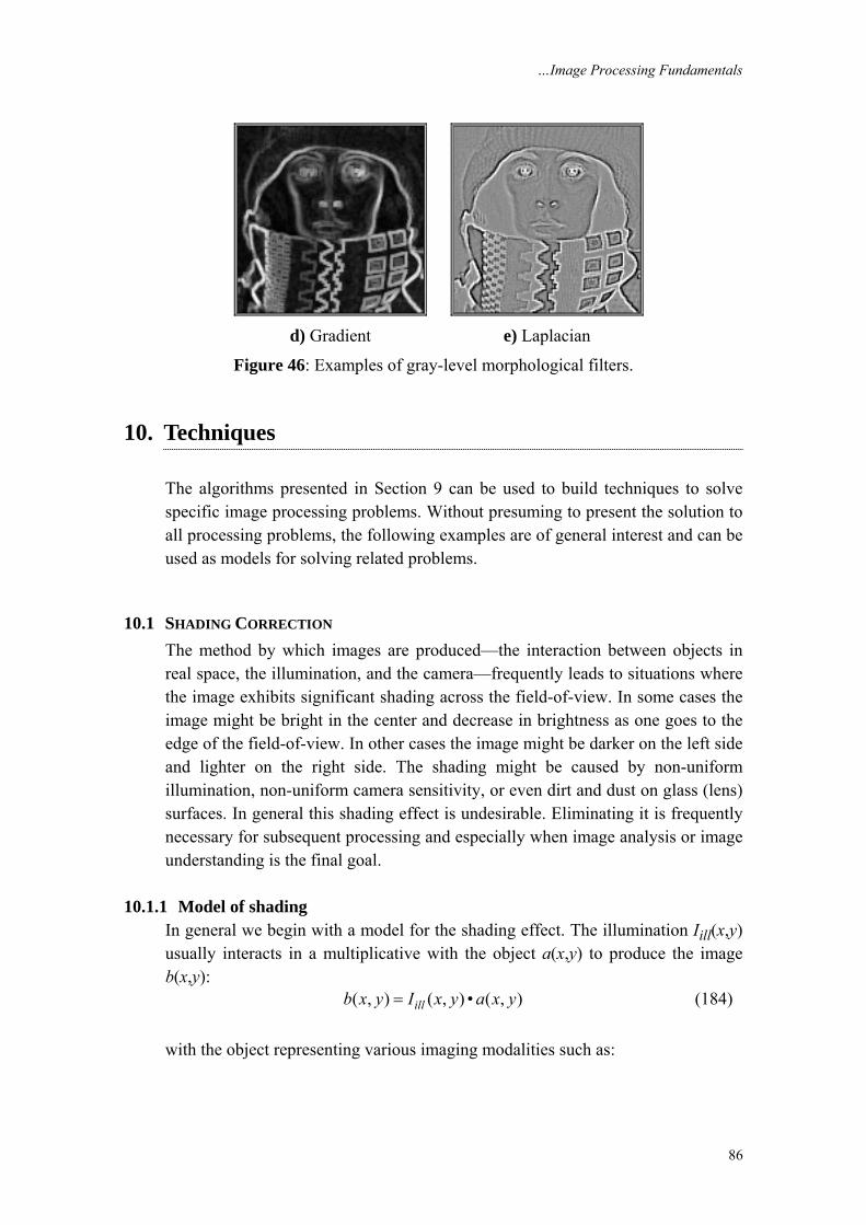
…Image Processing Fundamentals
86
d) Gradient e) Laplacian
Figure 46: Examples of gray-level morphological filters.
10. Techniques The algorithms presented in Section 9 can be used to build techniques to solve specific image processing problems. Without presuming to present the solution to all processing problems, the following examples are of general interest and can be used as models for solving related problems.
10.1 SHADING CORRECTION The method by which images are produced—the interaction between objects in real space, the illumination, and the camera—frequently leads to situations where the image exhibits significant shading across the field-of-view. In some cases the image might be bright in the center and decrease in brightness as one goes to the edge of the field-of-view. In other cases the image might be darker on the left side and lighter on the right side. The shading might be caused by non-uniform illumination, non-uniform camera sensitivity, or even dirt and dust on glass (lens) surfaces. In general this shading effect is undesirable. Eliminating it is frequently necessary for subsequent processing and especially when image analysis or image understanding is the final goal.
10.1.1 Model of shading In general we begin with a model for the shading effect. The illumination Iill(x,y) usually interacts in a multiplicative with the object a(x,y) to produce the image b(x,y): ( , ) ( , ) • ( , )illb x y I x y a x y= (184) with the object representing various imaging modalities such as:
…Image Processing Fundamentals
87
( , )
( , ) reflectance model
( , ) 10 absorption model
( , ) fluorescence model
OD x y
r x y
a x y
c x y
−
⎧⎪⎪⎪= ⎨⎪⎪⎪⎩
(185)
where at position (x,y), r(x,y) is the reflectance, OD(x,y) is the optical density, and c(x,y) is the concentration of fluorescent material. Parenthetically, we note that the fluorescence model only holds for low concentrations. The camera may then contribute gain and offset terms, as in eq. (74), so that:
Total shading – [ , ] [ , ]• [ , ] [ , ]
[ , ]• [ , ]• [ , ] [ , ]ill
c m n gain m n b m n offset m ngain m n I m n a m n offset m n
= += +
(186)
In general we assume that Iill[m,n] is slowly varying compared to a[m,n].
10.1.2 Estimate of shading We distinguish between two cases for the determination of a[m,n] starting from c[m,n]. In both cases we intend to estimate the shading terms {gain[m,n]•Iill[m,n]} and {offset[m,n]}. While in the first case we assume that we have only the recorded image c[m,n] with which to work, in the second case we assume that we can record two, additional, calibration images. • A posteriori estimate – In this case we attempt to extract the shading estimate from c[m,n]. The most common possibilities are the following. Lowpass filtering – We compute a smoothed version of c[m,n] where the smoothing is large compared to the size of the objects in the image. This smoothed version is intended to be an estimate of the background of the image. We then subtract the smoothed version from c[m,n] and then restore the desired DC value. In formula: Lowpass – { }ˆ[ , ] [ , ] [ , ]a m n c m n LowPass c m n constant= − + (187)
where ˆ[ , ]a m n is the estimate of a[m,n]. Choosing the appropriate lowpass filter means knowing the appropriate spatial frequencies in the Fourier domain where the shading terms dominate. Homomorphic filtering – We note that, if the offset[m,n] = 0, then c[m,n] consists solely of multiplicative terms. Further, the term {gain[m,n]•Iill[m,n]} is slowly varying while a[m,n] presumably is not. We therefore take the logarithm of c[m,n]
…Image Processing Fundamentals
88
to produce two terms one of which is low frequency and one of which is high frequency. We suppress the shading by high pass filtering the logarithm of c[m,n] and then take the exponent (inverse logarithm) to restore the image. This procedure is based on homomorphic filtering as developed by Oppenheim, Schafer and Stockham [34]. In formula:
{ }
{ }{ } { }{ }{ }{ }
) [ , ] [ , ]• [ , ]• [ , ]
) ln [ , ] ln [ , ]• [ , ] ln [ , ]
) ln [ , ] ln [ , ]
ˆ) [ , ] exp ln [ , ]
ill
illrapidly varyingslowly varying
i c m n gain m n I m n a m n
ii c m n gain m n I m n a m n
iii HighPass c m n a m n
iv a m n HighPass c m n
=
⎧ ⎫ ⎧ ⎫⎪ ⎪ ⎪ ⎪= +⎨ ⎬ ⎨ ⎬⎪ ⎪ ⎪ ⎪⎩ ⎭⎩ ⎭
≈
=
(188)
Morphological filtering – We again compute a smoothed version of c[m,n] where the smoothing is large compared to the size of the objects in the image but this time using morphological smoothing as in eq. (181). This smoothed version is the estimate of the background of the image. We then subtract the smoothed version from c[m,n] and then restore the desired DC value. In formula: { }ˆ[ , ] [ , ] [ , ]a m n c m n MorphSmooth c m n constant= − + (189)
Choosing the appropriate morphological filter window means knowing (or estimating) the size of the largest objects of interest. • A priori estimate – If it is possible to record test (calibration) images through the cameras system, then the most appropriate technique for the removal of shading effects is to record two images – BLACK[m,n] and WHITE[m,n]. The BLACK image is generated by covering the lens leading to b[m,n] = 0 which in turn leads to BLACK[m,n] = offset[m,n]. The WHITE image is generated by using a[m,n] = 1 which gives WHITE[m,n] = gain[m,n]•Iill[m,n] + offset[m,n]. The correction then becomes:
[ , ] [ , ]ˆ[ , ] •[ , ] [ , ]
BLACK
WHITE BLACK
c m n m na m n constantm n m n
−=
− (190)
The constant term is chosen to produce the desired dynamic range. The effects of these various techniques on the data from Figure 45 are shown in Figure 47. The shading is a simple, linear ramp increasing from left to right; the objects consist of Gaussian peaks of varying widths.
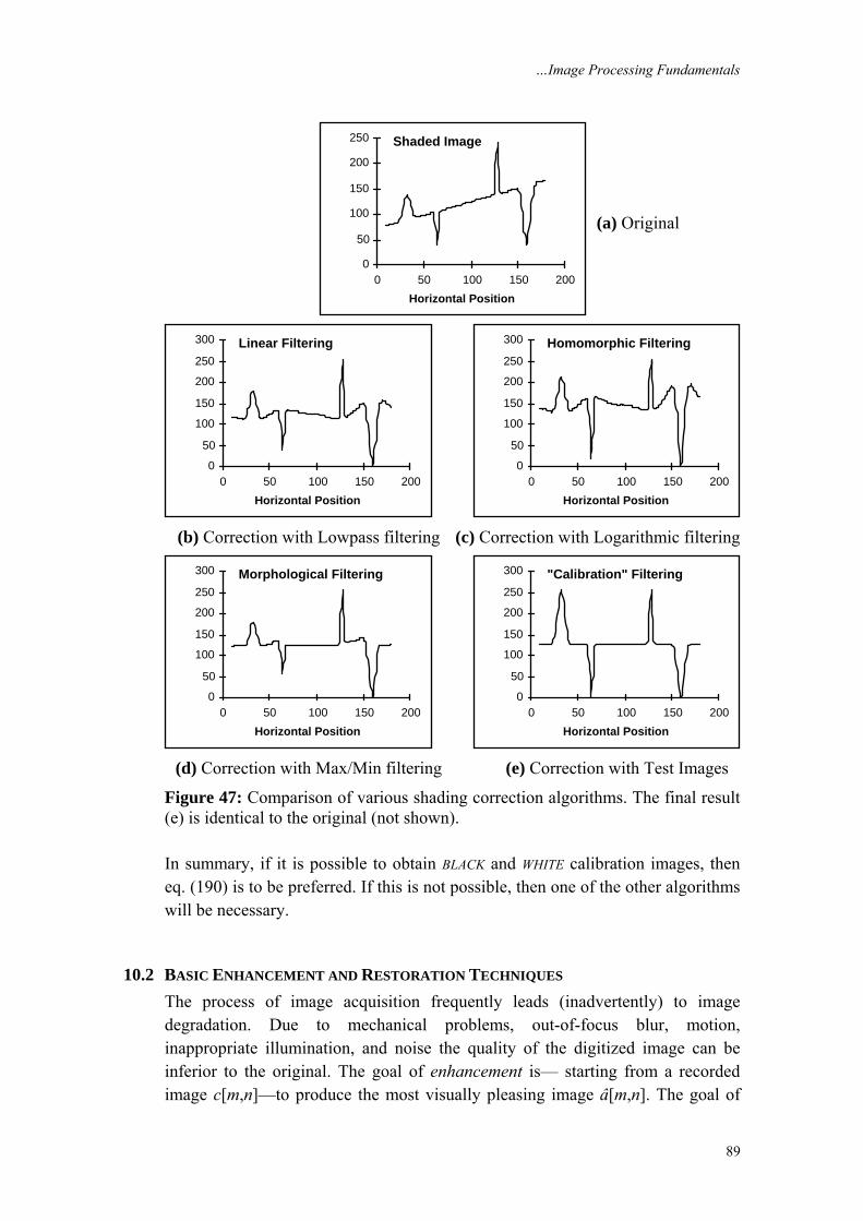
…Image Processing Fundamentals
89
0
50
100
150
200
250
0 50 100 150 200Horizontal Position
Shaded Image
(a) Original
0
50
100
150
200
250
300
0 50 100 150 200Horizontal Position
Linear Filtering
0
50
100
150
200
250
300
0 50 100 150 200Horizontal Position
Homomorphic Filtering
(b) Correction with Lowpass filtering (c) Correction with Logarithmic filtering
0
50
100
150
200
250
300
0 50 100 150 200Horizontal Position
Morphological Filtering
0
50
100
150
200
250
300
0 50 100 150 200Horizontal Position
"Calibration" Filtering
(d) Correction with Max/Min filtering (e) Correction with Test Images
Figure 47: Comparison of various shading correction algorithms. The final result (e) is identical to the original (not shown). In summary, if it is possible to obtain BLACK and WHITE calibration images, then eq. (190) is to be preferred. If this is not possible, then one of the other algorithms will be necessary.
10.2 BASIC ENHANCEMENT AND RESTORATION TECHNIQUES The process of image acquisition frequently leads (inadvertently) to image degradation. Due to mechanical problems, out-of-focus blur, motion, inappropriate illumination, and noise the quality of the digitized image can be inferior to the original. The goal of enhancement is— starting from a recorded image c[m,n]—to produce the most visually pleasing image â[m,n]. The goal of

…Image Processing Fundamentals
90
restoration is—starting from a recorded image c[m,n]—to produce the best possible estimate â[m,n] of the original image a[m,n]. The goal of enhancement is beauty; the goal of restoration is truth. The measure of success in restoration is usually an error measure between the original a[m,n] and the estimate â[m,n]: E{â[m,n], a[m,n]}. No mathematical error function is known that corresponds to human perceptual assessment of error. The mean-square error function is commonly used because: 1. It is easy to compute; 2. It is differentiable implying that a minimum can be sought; 3. It corresponds to “signal energy” in the total error, and; 4. It has nice properties vis à vis Parseval’s theorem, eqs. (22) and (23). The mean-square error is defined by:
{ }1 1
2
0 0
1ˆ ˆ, [ , ] [ , ]M N
m na a a m n a m n
MN
− −
= =
= −∑ ∑E (191)
In some techniques an error measure will not be necessary; in others it will be essential for evaluation and comparative purposes.
10.2.1 Unsharp masking A well-known technique from photography to improve the visual quality of an image is to enhance the edges of the image. The technique is called unsharp masking. Edge enhancement means first isolating the edges in an image, amplifying them, and then adding them back into the image. Examination of Figure 33 shows that the Laplacian is a mechanism for isolating the gray level edges. This leads immediately to the technique: ( )2ˆ[ , ] [ , ] • [ , ]a m n a m n k a m n= − ∇ (192)
The term k is the amplifying term and k > 0. The effect of this technique is shown in Figure 48. The Laplacian used to produce Figure 48 is given by eq. (120) and the amplification term k = 1.
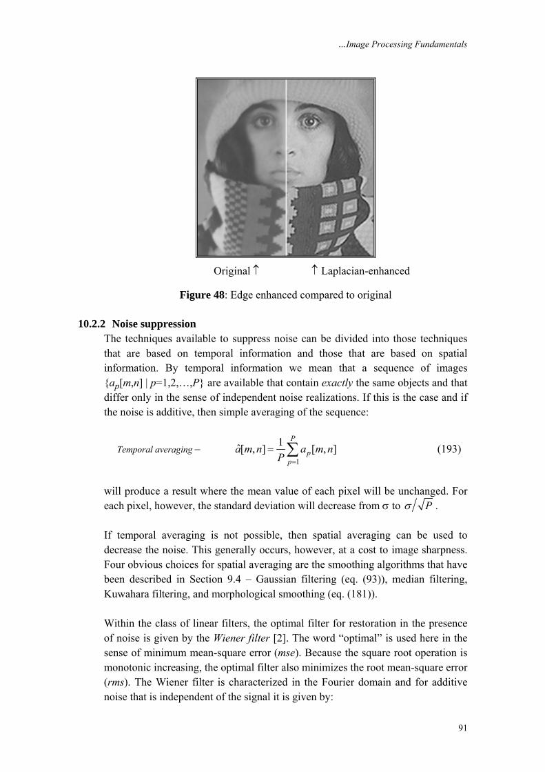
…Image Processing Fundamentals
91
Original ↑ ↑ Laplacian-enhanced
Figure 48: Edge enhanced compared to original
10.2.2 Noise suppression The techniques available to suppress noise can be divided into those techniques that are based on temporal information and those that are based on spatial information. By temporal information we mean that a sequence of images {ap[m,n] | p=1,2,…,P} are available that contain exactly the same objects and that differ only in the sense of independent noise realizations. If this is the case and if the noise is additive, then simple averaging of the sequence:
Temporal averaging – 1
1ˆ[ , ] [ , ]P
pp
a m n a m nP =
= ∑ (193)
will produce a result where the mean value of each pixel will be unchanged. For each pixel, however, the standard deviation will decrease from σ to Pσ . If temporal averaging is not possible, then spatial averaging can be used to decrease the noise. This generally occurs, however, at a cost to image sharpness. Four obvious choices for spatial averaging are the smoothing algorithms that have been described in Section 9.4 – Gaussian filtering (eq. (93)), median filtering, Kuwahara filtering, and morphological smoothing (eq. (181)). Within the class of linear filters, the optimal filter for restoration in the presence of noise is given by the Wiener filter [2]. The word “optimal” is used here in the sense of minimum mean-square error (mse). Because the square root operation is monotonic increasing, the optimal filter also minimizes the root mean-square error (rms). The Wiener filter is characterized in the Fourier domain and for additive noise that is independent of the signal it is given by:
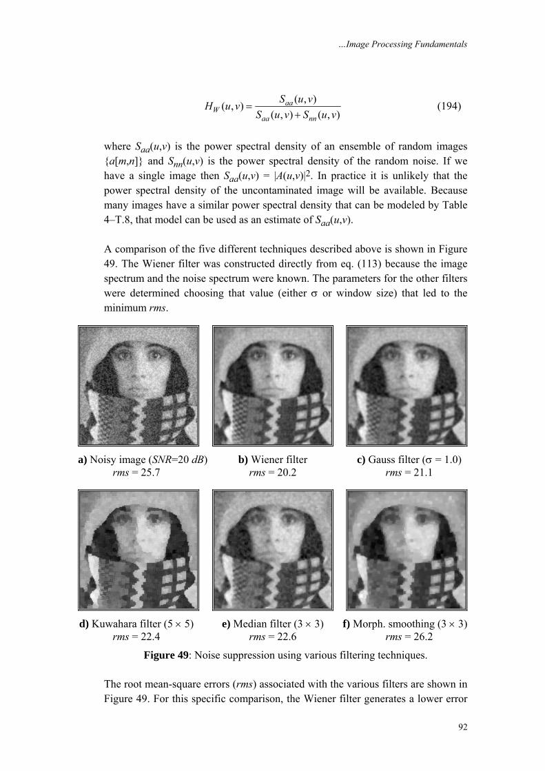
…Image Processing Fundamentals
92
( , )( , )( , ) ( , )
aaW
aa nn
S u vH u vS u v S u v
=+
(194)
where Saa(u,v) is the power spectral density of an ensemble of random images {a[m,n]} and Snn(u,v) is the power spectral density of the random noise. If we have a single image then Saa(u,v) = |A(u,v)|2. In practice it is unlikely that the power spectral density of the uncontaminated image will be available. Because many images have a similar power spectral density that can be modeled by Table 4–T.8, that model can be used as an estimate of Saa(u,v). A comparison of the five different techniques described above is shown in Figure 49. The Wiener filter was constructed directly from eq. (113) because the image spectrum and the noise spectrum were known. The parameters for the other filters were determined choosing that value (either σ or window size) that led to the minimum rms.
a) Noisy image (SNR=20 dB) b) Wiener filter c) Gauss filter (σ = 1.0) rms = 25.7 rms = 20.2 rms = 21.1
d) Kuwahara filter (5 × 5) e) Median filter (3 × 3) f) Morph. smoothing (3 × 3) rms = 22.4 rms = 22.6 rms = 26.2
Figure 49: Noise suppression using various filtering techniques. The root mean-square errors (rms) associated with the various filters are shown in Figure 49. For this specific comparison, the Wiener filter generates a lower error
…Image Processing Fundamentals
93
than any of the other procedures that are examined here. The two linear procedures, Wiener filtering and Gaussian filtering, performed slightly better than the three non-linear alternatives.
10.2.3 Distortion suppression The model presented above—an image distorted solely by noise—is not, in general, sophisticated enough to describe the true nature of distortion in a digital image. A more realistic model includes not only the noise but also a model for the distortion induced by lenses, finite apertures, possible motion of the camera and/or an object, and so forth. One frequently used model is of an image a[m,n] distorted by a linear, shift-invariant system ho[m,n] (such as a lens) and then contaminated by noise κ[m,n]. Various aspects of ho[m,n] and κ[m,n] have been discussed in earlier sections. The most common combination of these is the additive model: ( )[ , ] [ , ] [ , ] [ , ]oc m n a m n h m n m nκ= ⊗ + (195)
The restoration procedure that is based on linear filtering coupled to a minimum mean-square error criterion again produces a Wiener filter [2]:
*
2
*
2
( , ) ( , )( , )( , ) ( , ) ( , )
( , )( , )( , )( , )
o aaW
o aa nn
o
nno
aa
H u v S u vH u vH u v S u v S u v
H u vS u vH u vS u v
=+
=+
(196)
Once again Saa(u,v) is the power spectral density of an image, Snn(u,v) is the power spectral density of the noise, and Ho(u,v) = F{ho[m,n]}. Examination of this formula for some extreme cases can be useful. For those frequencies where Saa(u,v) >> Snn(u,v), where the signal spectrum dominates the noise spectrum, the Wiener filter is given by 1/Ho(u,v), the inverse filter solution. For those frequencies where Saa(u,v) << Snn(u,v), where the noise spectrum dominates the signal spectrum, the Wiener filter is proportional to Ho*(u,v), the matched filter solution. For those frequencies where Ho(u,v) = 0, the Wiener filter HW(u,v) = 0 preventing overflow. The Wiener filter is a solution to the restoration problem based upon the hypothesized use of a linear filter and the minimum mean-square (or rms) error criterion. In the example below the image a[m,n] was distorted by a bandpass
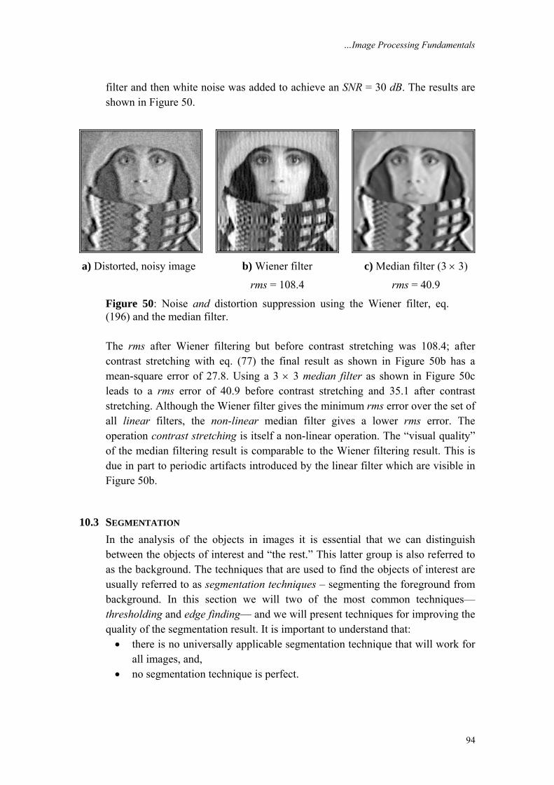
…Image Processing Fundamentals
94
filter and then white noise was added to achieve an SNR = 30 dB. The results are shown in Figure 50.
a) Distorted, noisy image b) Wiener filter c) Median filter (3 × 3)
rms = 108.4 rms = 40.9
Figure 50: Noise and distortion suppression using the Wiener filter, eq. (196) and the median filter. The rms after Wiener filtering but before contrast stretching was 108.4; after contrast stretching with eq. (77) the final result as shown in Figure 50b has a mean-square error of 27.8. Using a 3 × 3 median filter as shown in Figure 50c leads to a rms error of 40.9 before contrast stretching and 35.1 after contrast stretching. Although the Wiener filter gives the minimum rms error over the set of all linear filters, the non-linear median filter gives a lower rms error. The operation contrast stretching is itself a non-linear operation. The “visual quality” of the median filtering result is comparable to the Wiener filtering result. This is due in part to periodic artifacts introduced by the linear filter which are visible in Figure 50b.
10.3 SEGMENTATION In the analysis of the objects in images it is essential that we can distinguish between the objects of interest and “the rest.” This latter group is also referred to as the background. The techniques that are used to find the objects of interest are usually referred to as segmentation techniques – segmenting the foreground from background. In this section we will two of the most common techniques—thresholding and edge finding— and we will present techniques for improving the quality of the segmentation result. It is important to understand that:
• there is no universally applicable segmentation technique that will work for all images, and,
• no segmentation technique is perfect.
…Image Processing Fundamentals
95
10.3.1 Thresholding This technique is based upon a simple concept. A parameter θ called the brightness threshold is chosen and applied to the image a[m,n] as follows:
[ , ] [ , ] 1
[ , ] 0a m n a m n object
a m n backgroundθ≥ = =
= =IfElse
(197)
This version of the algorithm assumes that we are interested in light objects on a dark background. For dark objects on a light background we would use:
[ , ] [ , ] 1
[ , ] 0a m n a m n object
a m n backgroundθ< = =
= =IfElse
(198)
The output is the label “object” or “background” which, due to its dichotomous nature, can be represented as a Boolean variable “1” or “0”. In principle, the test condition could be based upon some other property than simple brightness (for example, If (Redness{a[m,n]} ≥ θred), but the concept is clear. The central question in thresholding then becomes: How do we choose the threshold θ? While there is no universal procedure for threshold selection that is guaranteed to work on all images, there are a variety of alternatives. • Fixed threshold – One alternative is to use a threshold that is chosen independently of the image data. If it is known that one is dealing with very high-contrast images where the objects are very dark and the background is homogeneous (Section 10.1) and very light, then a constant threshold of 128 on a scale of 0 to 255 might be sufficiently accurate. By accuracy we mean that the number of falsely-classified pixels should be kept to a minimum. • Histogram-derived thresholds – In most cases the threshold is chosen from the brightness histogram of the region or image that we wish to segment. (See Sections 3.5.2 and 9.1.) An image and its associated brightness histogram are shown in Figure 51. A variety of techniques have been devised to automatically choose a threshold starting from the gray-value histogram, {h[b] | b = 0, 1, … , 2B–1}. Some of the most common ones are presented below. Many of these algorithms can benefit from a smoothing of the raw histogram data to remove small fluctuations but the smoothing algorithm must not shift the peak positions. This translates into a zero-phase smoothing algorithm given below where typical values for W are 3 or 5:
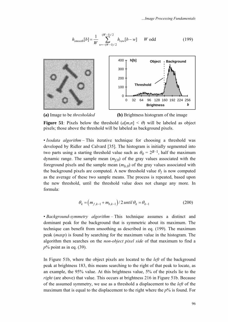
…Image Processing Fundamentals
96
( 1) / 2
( 1) / 2
1[ ] [ ] oddW
smooth raww W
h b h b w WW
−
=− −= −∑ (199)
0
100
200
300
400
0 32 64 96 128 160 192 224 256Brightness
Threshold
Object Backgroundh[b]
b
(a) Image to be thresholded (b) Brightness histogram of the image
Figure 51: Pixels below the threshold (a[m,n] < θ) will be labeled as object pixels; those above the threshold will be labeled as background pixels. • Isodata algorithm – This iterative technique for choosing a threshold was developed by Ridler and Calvard [35]. The histogram is initially segmented into two parts using a starting threshold value such as θ0 = 2B–1, half the maximum dynamic range. The sample mean (mf,0) of the gray values associated with the foreground pixels and the sample mean (mb,0) of the gray values associated with the background pixels are computed. A new threshold value θ1 is now computed as the average of these two sample means. The process is repeated, based upon the new threshold, until the threshold value does not change any more. In formula: ( ), 1 , 1 1/ 2 k f k b k k km m untilθ θ θ− − −= + = (200)
• Background-symmetry algorithm – This technique assumes a distinct and dominant peak for the background that is symmetric about its maximum. The technique can benefit from smoothing as described in eq. (199). The maximum peak (maxp) is found by searching for the maximum value in the histogram. The algorithm then searches on the non-object pixel side of that maximum to find a p% point as in eq. (39). In Figure 51b, where the object pixels are located to the left of the background peak at brightness 183, this means searching to the right of that peak to locate, as an example, the 95% value. At this brightness value, 5% of the pixels lie to the right (are above) that value. This occurs at brightness 216 in Figure 51b. Because of the assumed symmetry, we use as a threshold a displacement to the left of the maximum that is equal to the displacement to the right where the p% is found. For
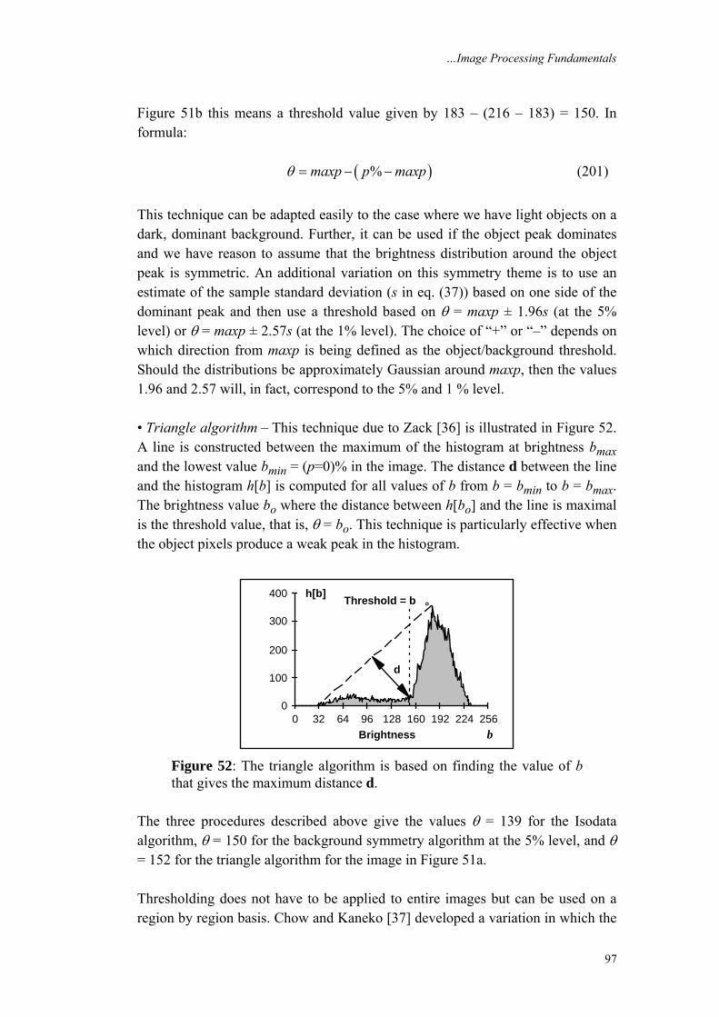
…Image Processing Fundamentals
97
Figure 51b this means a threshold value given by 183 – (216 – 183) = 150. In formula: ( )%maxp p maxpθ = − − (201)
This technique can be adapted easily to the case where we have light objects on a dark, dominant background. Further, it can be used if the object peak dominates and we have reason to assume that the brightness distribution around the object peak is symmetric. An additional variation on this symmetry theme is to use an estimate of the sample standard deviation (s in eq. (37)) based on one side of the dominant peak and then use a threshold based on θ = maxp ± 1.96s (at the 5% level) or θ = maxp ± 2.57s (at the 1% level). The choice of “+” or “–” depends on which direction from maxp is being defined as the object/background threshold. Should the distributions be approximately Gaussian around maxp, then the values 1.96 and 2.57 will, in fact, correspond to the 5% and 1 % level. • Triangle algorithm – This technique due to Zack [36] is illustrated in Figure 52. A line is constructed between the maximum of the histogram at brightness bmax and the lowest value bmin = (p=0)% in the image. The distance d between the line and the histogram h[b] is computed for all values of b from b = bmin to b = bmax. The brightness value bo where the distance between h[bo] and the line is maximal is the threshold value, that is, θ = bo. This technique is particularly effective when the object pixels produce a weak peak in the histogram.
0
100
200
300
400
0 32 64 96 128 160 192 224 256Brightness
Threshold = b o
d
b
h[b]
Figure 52: The triangle algorithm is based on finding the value of b that gives the maximum distance d.
The three procedures described above give the values θ = 139 for the Isodata algorithm, θ = 150 for the background symmetry algorithm at the 5% level, and θ = 152 for the triangle algorithm for the image in Figure 51a. Thresholding does not have to be applied to entire images but can be used on a region by region basis. Chow and Kaneko [37] developed a variation in which the
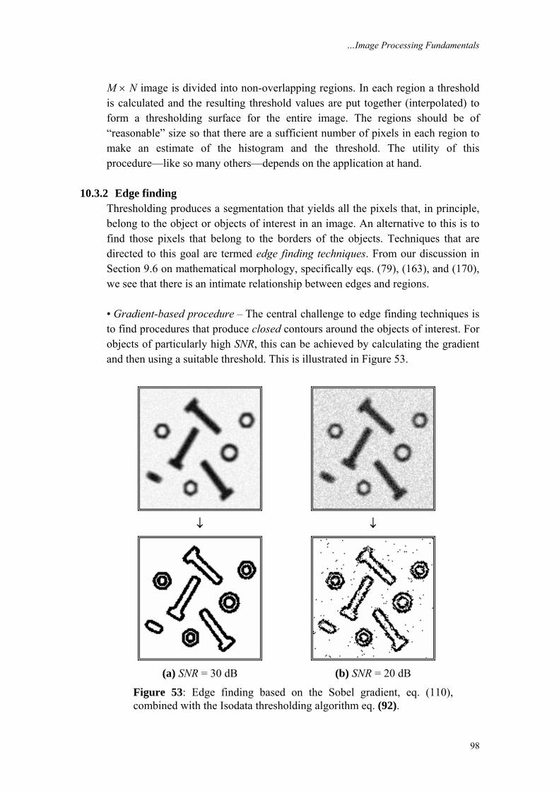
…Image Processing Fundamentals
98
M × N image is divided into non-overlapping regions. In each region a threshold is calculated and the resulting threshold values are put together (interpolated) to form a thresholding surface for the entire image. The regions should be of “reasonable” size so that there are a sufficient number of pixels in each region to make an estimate of the histogram and the threshold. The utility of this procedure—like so many others—depends on the application at hand.
10.3.2 Edge finding Thresholding produces a segmentation that yields all the pixels that, in principle, belong to the object or objects of interest in an image. An alternative to this is to find those pixels that belong to the borders of the objects. Techniques that are directed to this goal are termed edge finding techniques. From our discussion in Section 9.6 on mathematical morphology, specifically eqs. (79), (163), and (170), we see that there is an intimate relationship between edges and regions. • Gradient-based procedure – The central challenge to edge finding techniques is to find procedures that produce closed contours around the objects of interest. For objects of particularly high SNR, this can be achieved by calculating the gradient and then using a suitable threshold. This is illustrated in Figure 53.
↓ ↓
(a) SNR = 30 dB (b) SNR = 20 dB
Figure 53: Edge finding based on the Sobel gradient, eq. (110), combined with the Isodata thresholding algorithm eq. (92).
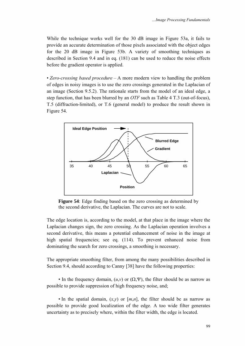
…Image Processing Fundamentals
99
While the technique works well for the 30 dB image in Figure 53a, it fails to provide an accurate determination of those pixels associated with the object edges for the 20 dB image in Figure 53b. A variety of smoothing techniques as described in Section 9.4 and in eq. (181) can be used to reduce the noise effects before the gradient operator is applied. • Zero-crossing based procedure – A more modern view to handling the problem of edges in noisy images is to use the zero crossings generated in the Laplacian of an image (Section 9.5.2). The rationale starts from the model of an ideal edge, a step function, that has been blurred by an OTF such as Table 4 T.3 (out-of-focus), T.5 (diffraction-limited), or T.6 (general model) to produce the result shown in Figure 54.
35 40 45 50 55 60 65
Position
Blurred Edge
Gradient
Laplacian
Ideal Edge Position
Figure 54: Edge finding based on the zero crossing as determined by the second derivative, the Laplacian. The curves are not to scale.
The edge location is, according to the model, at that place in the image where the Laplacian changes sign, the zero crossing. As the Laplacian operation involves a second derivative, this means a potential enhancement of noise in the image at high spatial frequencies; see eq. (114). To prevent enhanced noise from dominating the search for zero crossings, a smoothing is necessary. The appropriate smoothing filter, from among the many possibilities described in Section 9.4, should according to Canny [38] have the following properties: • In the frequency domain, (u,v) or (Ω,Ψ), the filter should be as narrow as possible to provide suppression of high frequency noise, and; • In the spatial domain, (x,y) or [m,n], the filter should be as narrow as possible to provide good localization of the edge. A too wide filter generates uncertainty as to precisely where, within the filter width, the edge is located.
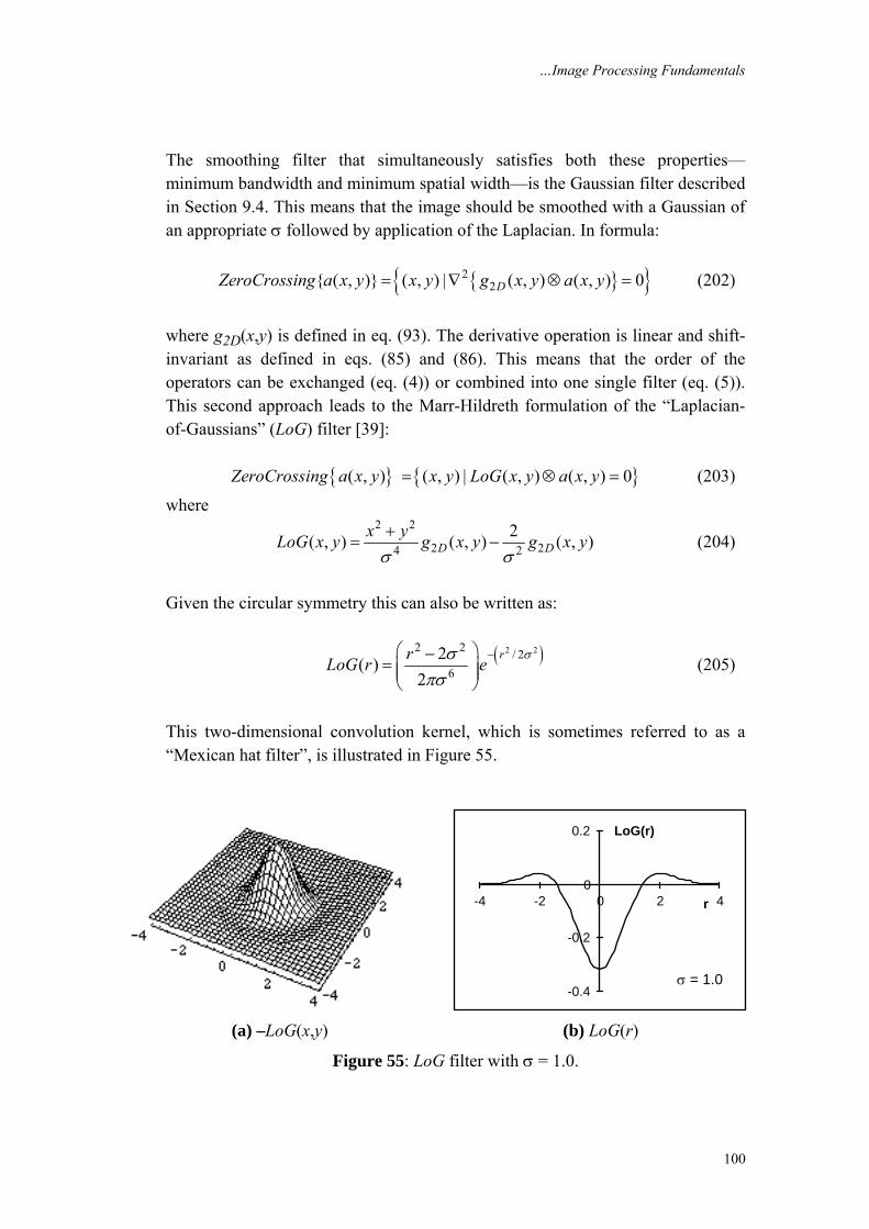
…Image Processing Fundamentals
100
The smoothing filter that simultaneously satisfies both these properties—minimum bandwidth and minimum spatial width—is the Gaussian filter described in Section 9.4. This means that the image should be smoothed with a Gaussian of an appropriate σ followed by application of the Laplacian. In formula: { }{ }2
2{ ( , )} ( , ) | ( , ) ( , ) 0DZeroCrossing a x y x y g x y a x y= ∇ ⊗ = (202)
where g2D(x,y) is defined in eq. (93). The derivative operation is linear and shift-invariant as defined in eqs. (85) and (86). This means that the order of the operators can be exchanged (eq. (4)) or combined into one single filter (eq. (5)). This second approach leads to the Marr-Hildreth formulation of the “Laplacian-of-Gaussians” (LoG) filter [39]: { } { }( , ) ( , ) | ( , ) ( , ) 0ZeroCrossing a x y x y LoG x y a x y= ⊗ = (203)
where
2 2
2 24 22( , ) ( , ) ( , )D D
x yLoG x y g x y g x yσ σ+
= − (204)
Given the circular symmetry this can also be written as:
( )2 22 2 / 26
2( )2
rrLoG r eσσ
πσ−⎛ ⎞−
= ⎜ ⎟⎜ ⎟⎝ ⎠
(205)
This two-dimensional convolution kernel, which is sometimes referred to as a “Mexican hat filter”, is illustrated in Figure 55.
-0.4
-0.2
0
0.2
-4 -2 0 2 4r
σ = 1.0
LoG(r)
(a) –LoG(x,y) (b) LoG(r)
Figure 55: LoG filter with σ = 1.0.
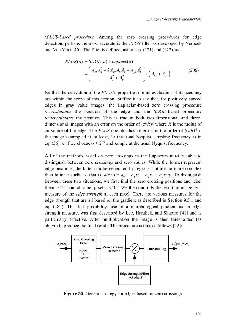
…Image Processing Fundamentals
101
•PLUS-based procedure – Among the zero crossing procedures for edge detection, perhaps the most accurate is the PLUS filter as developed by Verbeek and Van Vliet [40]. The filter is defined, using eqs. (121) and (122), as:
( )2 2
2 2
( ) ( ) ( )
2xx x xy x y yy yxx yy
x y
PLUS a SDGD a Laplace a
A A A A A A AA A
A A
= +
⎛ ⎞+ +⎜ ⎟= + +⎜ ⎟+⎝ ⎠
(206)
Neither the derivation of the PLUS’s properties nor an evaluation of its accuracy are within the scope of this section. Suffice it to say that, for positively curved edges in gray value images, the Laplacian-based zero crossing procedure overestimates the position of the edge and the SDGD-based procedure underestimates the position. This is true in both two-dimensional and three-dimensional images with an error on the order of (σ/R)2 where R is the radius of curvature of the edge. The PLUS operator has an error on the order of (σ/R)4 if the image is sampled at, at least, 3× the usual Nyquist sampling frequency as in eq. (56) or if we choose σ ≥ 2.7 and sample at the usual Nyquist frequency. All of the methods based on zero crossings in the Laplacian must be able to distinguish between zero crossings and zero values. While the former represent edge positions, the latter can be generated by regions that are no more complex than bilinear surfaces, that is, a(x,y) = a0 + a1•x + a2•y + a3•x•y. To distinguish between these two situations, we first find the zero crossing positions and label them as “1” and all other pixels as “0”. We then multiply the resulting image by a measure of the edge strength at each pixel. There are various measures for the edge strength that are all based on the gradient as described in Section 9.5.1 and eq. (182). This last possibility, use of a morphological gradient as an edge strength measure, was first described by Lee, Haralick, and Shapiro [41] and is particularly effective. After multiplication the image is then thresholded (as above) to produce the final result. The procedure is thus as follows [42]:
a[m,n] edges[m,n]×Zero Crossing Detector
Zero Crossing Filter
• LoG • PLUS • other
Thresholding
Edge Strength Filter (Gradient)
Figure 56: General strategy for edges based on zero crossings.
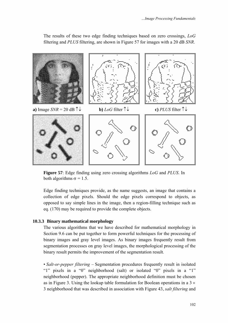
…Image Processing Fundamentals
102
The results of these two edge finding techniques based on zero crossings, LoG filtering and PLUS filtering, are shown in Figure 57 for images with a 20 dB SNR.
a) Image SNR = 20 dB ↑↓ b) LoG filter ↑↓ c) PLUS filter ↑↓
Figure 57: Edge finding using zero crossing algorithms LoG and PLUS. In both algorithms σ = 1.5. Edge finding techniques provide, as the name suggests, an image that contains a collection of edge pixels. Should the edge pixels correspond to objects, as opposed to say simple lines in the image, then a region-filling technique such as eq. (170) may be required to provide the complete objects.
10.3.3 Binary mathematical morphology The various algorithms that we have described for mathematical morphology in Section 9.6 can be put together to form powerful techniques for the processing of binary images and gray level images. As binary images frequently result from segmentation processes on gray level images, the morphological processing of the binary result permits the improvement of the segmentation result. • Salt-or-pepper filtering – Segmentation procedures frequently result in isolated “1” pixels in a “0” neighborhood (salt) or isolated “0” pixels in a “1” neighborhood (pepper). The appropriate neighborhood definition must be chosen as in Figure 3. Using the lookup table formulation for Boolean operations in a 3 × 3 neighborhood that was described in association with Figure 43, salt filtering and
…Image Processing Fundamentals
103
pepper filtering are straightforward to implement. We weight the different positions in the 3 × 3 neighborhood as follows:
4 3 2
5 0 1
6 7 8
16 8 432 1 264 128 256
w w wWeights w w w
w w w
= = =⎡ ⎤⎢ ⎥= = = =⎢ ⎥⎢ ⎥= = =⎣ ⎦
(207)
For a 3 × 3 window in a[m,n] with values “0” or “1” we then compute:
0 1 2
3 4 5
6 7 8
[ , ] [ 1, ] [ 1, 1][ , 1] [ 1, 1] [ 1, ][ 1, 1] [ , 1] [ 1, 1]
sum w a m n w a m n w a m nw a m n w a m n w a m nw a m n w a m n w a m n
= + + + + − +
− + − − + − +
− + + + + + −
(208)
The result, sum, is a number bounded by 0 ≤ sum ≤ 511. • Salt Filter – The 4-connected and 8-connected versions of this filter are the same and are given by the following procedure: i) Compute sum (209) ii) If ( (sum == 1) c[m,n] = 0 Else c[m,n] = a[m,n] • Pepper Filter – The 4-connected and 8-connected versions of this filter are the following procedures: 4-connected 8-connected i) Compute sum i) Compute sum (210) ii) If ( (sum == 170) ii) If ( (sum == 510) c[m,n] = 1 c[m,n] = 1 Else Else c[m,n] = a[m,n] c[m,n] = a[m,n] • Isolate objects with holes – To find objects with holes we can use the following procedure which is illustrated in Figure 58. i) Segment image to produce binary mask representation (211) ii) Compute skeleton without end pixels – eq. (169) iii) Use salt filter to remove single skeleton pixels iv) Propagate remaining skeleton pixels into original binary mask – eq. (170)
…Image Processing Fundamentals
104
a) Binary image b) Skeleton after salt filter c) Objects with holes
Figure 58: Isolation of objects with holes using morphological operations. The binary objects are shown in gray and the skeletons, after application of the salt filter, are shown as a black overlay on the binary objects. Note that this procedure uses no parameters other then the fundamental choice of connectivity; it is free from “magic numbers.” In the example shown in Figure 58, the 8-connected definition was used as well as the structuring element B = N8. • Filling holes in objects – To fill holes in objects we use the following procedure which is illustrated in Figure 59. i) Segment image to produce binary representation of objects (212) ii) Compute complement of binary image as a mask image iii) Generate a seed image as the border of the image iv) Propagate the seed into the mask – eq. (97) v) Complement result of propagation to produce final result
a) Mask and Seed images b) Objects with holes filled
Figure 59: Filling holes in objects. The mask image is illustrated in gray in Figure 59a and the seed image is shown in black in that same illustration. When the object pixels are specified with a connectivity of C = 8, then the propagation into the mask (background) image
…Image Processing Fundamentals
105
should be performed with a connectivity of C = 4, that is, dilations with the structuring element B = N4. This procedure is also free of “magic numbers.” • Removing border-touching objects – Objects that are connected to the image border are not suitable for analysis. To eliminate them we can use a series of morphological operations that are illustrated in Figure 60. i) Segment image to produce binary mask image of objects (213) ii) Generate a seed image as the border of the image iv) Propagate the seed into the mask – eq. (97) v) Compute XOR of the propagation result and the mask image as final result
a) Mask and Seed images b) Remaining objects
Figure 60: Removing objects touching borders. The mask image is illustrated in gray in Figure 60a and the seed image is shown in black in that same illustration. If the structuring element used in the propagation is B = N4, then objects are removed that are 4-connected with the image boundary. If B = N8 is used then objects that 8-connected with the boundary are removed. • Exo-skeleton – The exo-skeleton of a set of objects is the skeleton of the background that contains the objects. The exo-skeleton produces a partition of the image into regions each of which contains one object. The actual skeletonization (eq. (169)) is performed without the preservation of end pixels and with the border set to “0.” The procedure is described below and the result is illustrated in Figure 61. i) Segment image to produce binary image (214) ii) Compute complement of binary image iii) Compute skeleton using eq. (169)i+ii with border set to “0”
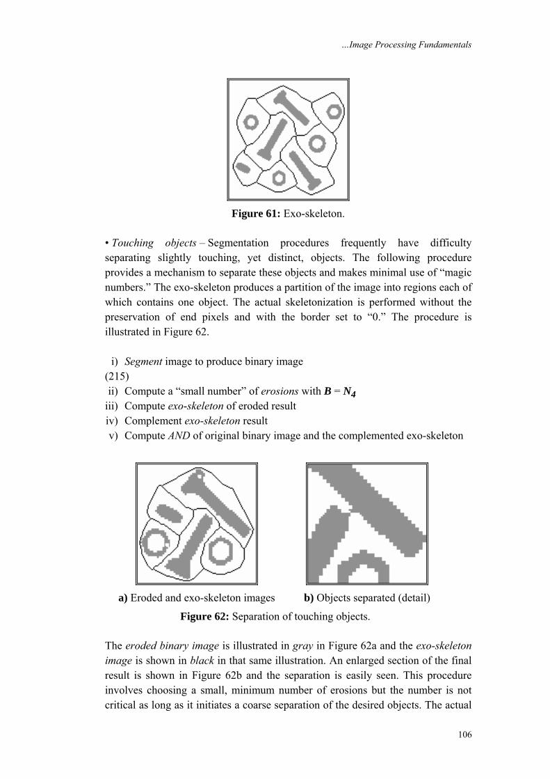
…Image Processing Fundamentals
106
Figure 61: Exo-skeleton.
• Touching objects – Segmentation procedures frequently have difficulty separating slightly touching, yet distinct, objects. The following procedure provides a mechanism to separate these objects and makes minimal use of “magic numbers.” The exo-skeleton produces a partition of the image into regions each of which contains one object. The actual skeletonization is performed without the preservation of end pixels and with the border set to “0.” The procedure is illustrated in Figure 62. i) Segment image to produce binary image (215) ii) Compute a “small number” of erosions with B = N4 iii) Compute exo-skeleton of eroded result iv) Complement exo-skeleton result v) Compute AND of original binary image and the complemented exo-skeleton
a) Eroded and exo-skeleton images b) Objects separated (detail)
Figure 62: Separation of touching objects. The eroded binary image is illustrated in gray in Figure 62a and the exo-skeleton image is shown in black in that same illustration. An enlarged section of the final result is shown in Figure 62b and the separation is easily seen. This procedure involves choosing a small, minimum number of erosions but the number is not critical as long as it initiates a coarse separation of the desired objects. The actual
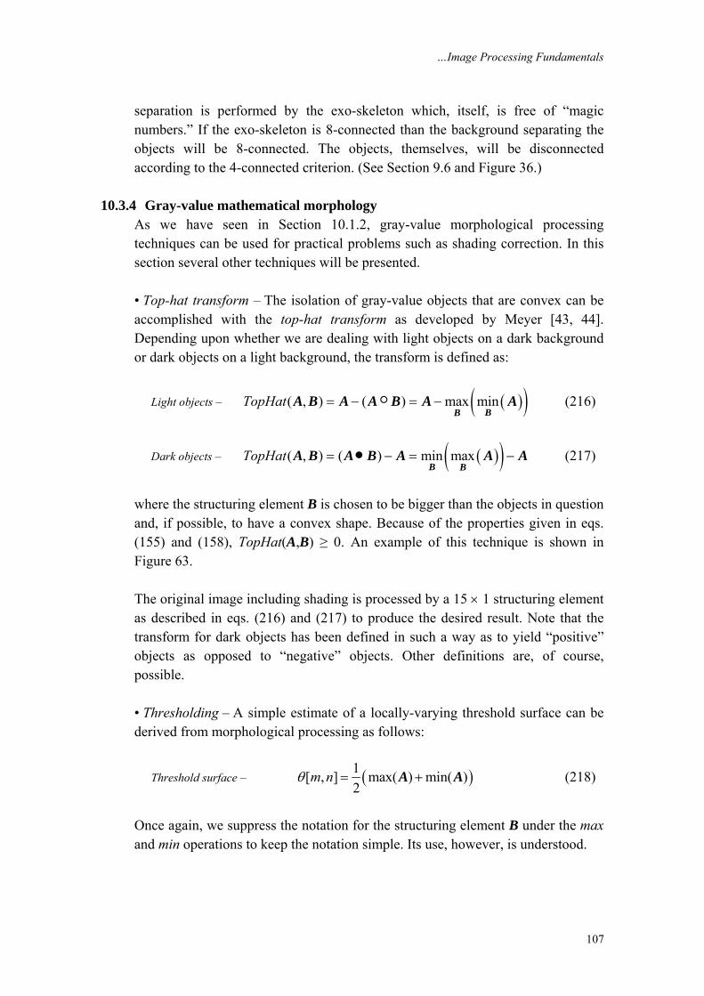
…Image Processing Fundamentals
107
separation is performed by the exo-skeleton which, itself, is free of “magic numbers.” If the exo-skeleton is 8-connected than the background separating the objects will be 8-connected. The objects, themselves, will be disconnected according to the 4-connected criterion. (See Section 9.6 and Figure 36.)
10.3.4 Gray-value mathematical morphology As we have seen in Section 10.1.2, gray-value morphological processing techniques can be used for practical problems such as shading correction. In this section several other techniques will be presented. • Top-hat transform – The isolation of gray-value objects that are convex can be accomplished with the top-hat transform as developed by Meyer [43, 44]. Depending upon whether we are dealing with light objects on a dark background or dark objects on a light background, the transform is defined as:
Light objects – ( )( )( , ) ( ) max minTopHat = − = −BB
A B A A B A A (216)
Dark objects – ( )( )( , ) ( ) min maxTopHat = − = −•B B
A B A B A A A (217)
where the structuring element B is chosen to be bigger than the objects in question and, if possible, to have a convex shape. Because of the properties given in eqs. (155) and (158), TopHat(A,B) ≥ 0. An example of this technique is shown in Figure 63. The original image including shading is processed by a 15 × 1 structuring element as described in eqs. (216) and (217) to produce the desired result. Note that the transform for dark objects has been defined in such a way as to yield “positive” objects as opposed to “negative” objects. Other definitions are, of course, possible. • Thresholding – A simple estimate of a locally-varying threshold surface can be derived from morphological processing as follows:
Threshold surface – ( )1[ , ] max( ) min( )2
m nθ = +A A (218)
Once again, we suppress the notation for the structuring element B under the max and min operations to keep the notation simple. Its use, however, is understood.
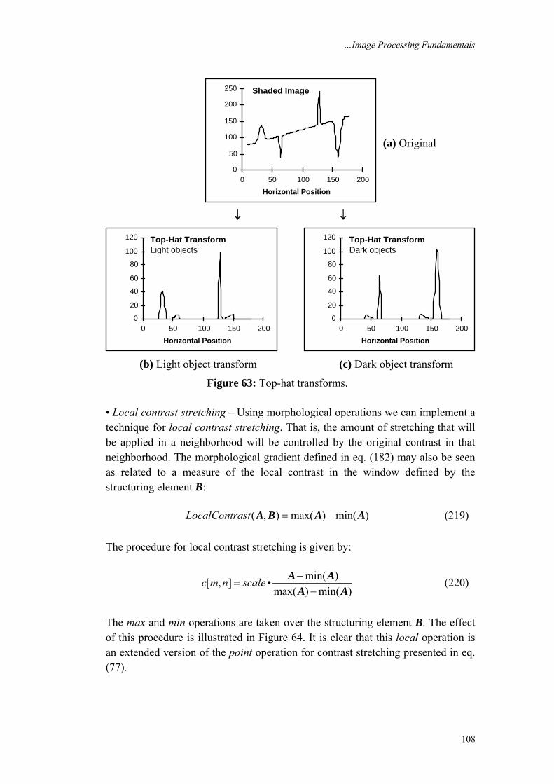
…Image Processing Fundamentals
108
0
50
100
150
200
250
0 50 100 150 200Horizontal Position
Shaded Image
(a) Original
↓ ↓
0
20
40
60
80
100
120
0 50 100 150 200Horizontal Position
Top-Hat TransformLight objects
0
20
40
60
80
100
120
0 50 100 150 200Horizontal Position
Top-Hat TransformDark objects
(b) Light object transform (c) Dark object transform
Figure 63: Top-hat transforms. • Local contrast stretching – Using morphological operations we can implement a technique for local contrast stretching. That is, the amount of stretching that will be applied in a neighborhood will be controlled by the original contrast in that neighborhood. The morphological gradient defined in eq. (182) may also be seen as related to a measure of the local contrast in the window defined by the structuring element B: ( , ) max( ) min( )LocalContrast = −A B A A (219) The procedure for local contrast stretching is given by:
min( )[ , ] •max( ) min( )
c m n scale −=
−A A
A A (220)
The max and min operations are taken over the structuring element B. The effect of this procedure is illustrated in Figure 64. It is clear that this local operation is an extended version of the point operation for contrast stretching presented in eq. (77).
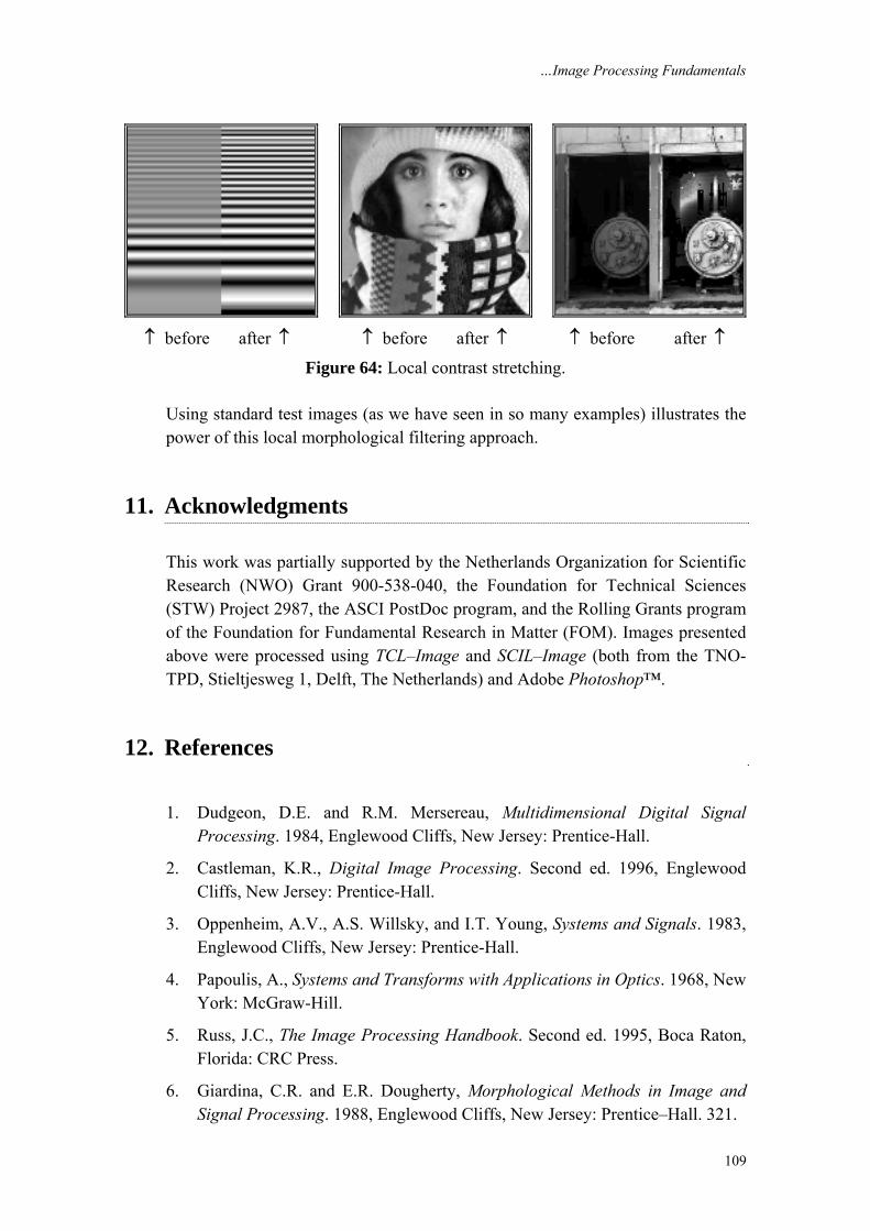
…Image Processing Fundamentals
109
↑ before after ↑ ↑ before after ↑ ↑ before after ↑
Figure 64: Local contrast stretching. Using standard test images (as we have seen in so many examples) illustrates the power of this local morphological filtering approach.
11. Acknowledgments This work was partially supported by the Netherlands Organization for Scientific Research (NWO) Grant 900-538-040, the Foundation for Technical Sciences (STW) Project 2987, the ASCI PostDoc program, and the Rolling Grants program of the Foundation for Fundamental Research in Matter (FOM). Images presented above were processed using TCL–Image and SCIL–Image (both from the TNO-TPD, Stieltjesweg 1, Delft, The Netherlands) and Adobe Photoshop™.
12. References
1. Dudgeon, D.E. and R.M. Mersereau, Multidimensional Digital Signal Processing. 1984, Englewood Cliffs, New Jersey: Prentice-Hall.
2. Castleman, K.R., Digital Image Processing. Second ed. 1996, Englewood Cliffs, New Jersey: Prentice-Hall.
3. Oppenheim, A.V., A.S. Willsky, and I.T. Young, Systems and Signals. 1983, Englewood Cliffs, New Jersey: Prentice-Hall.
4. Papoulis, A., Systems and Transforms with Applications in Optics. 1968, New York: McGraw-Hill.
5. Russ, J.C., The Image Processing Handbook. Second ed. 1995, Boca Raton, Florida: CRC Press.
6. Giardina, C.R. and E.R. Dougherty, Morphological Methods in Image and Signal Processing. 1988, Englewood Cliffs, New Jersey: Prentice–Hall. 321.

…Image Processing Fundamentals
110
7. Gonzalez, R.C. and R.E. Woods, Digital Image Processing. 1992, Reading, Massachusetts: Addison-Wesley. 716.
8. Goodman, J.W., Introduction to Fourier Optics. McGraw-Hill Physical and Quantum Electronics Series. 1968, New York: McGraw-Hill. 287.
9. Heijmans, H.J.A.M., Morphological Image Operators. Advances in Electronics and Electron Physics. 1994, Boston: Academic Press.
10. Hunt, R.W.G., The Reproduction of Colour in Photography, Printing & Television,. Fourth ed. 1987, Tolworth, England: Fountain Press.
11. Freeman, H., Boundary encoding and processing, in Picture Processing and Psychopictorics, B.S. Lipkin and A. Rosenfeld, Editors. 1970, Academic Press: New York. p. 241-266.
12. Stockham, T.G., Image Processing in the Context of a Visual Model. Proc. IEEE, 1972. 60: p. 828 - 842.
13. Murch, G.M., Visual and Auditory Perception. 1973, New York: Bobbs-Merrill Company, Inc. 403.
14. Frisby, J.P., Seeing: Illusion, Brain and Mind. 1980, Oxford, England: Oxford University Press. 160.
15. Blakemore, C. and F.W.C. Campbell, On the existence of neurons in the human visual system selectively sensitive to the orientation and size of retinal images. J. Physiology, 1969. 203: p. 237-260.
16. Born, M. and E. Wolf, Principles of Optics. Sixth ed. 1980, Oxford: Pergamon Press.
17. Young, I.T., Quantitative Microscopy. IEEE Engineering in Medicine and Biology, 1996. 15(1): p. 59-66.
18. Dorst, L. and A.W.M. Smeulders, Length estimators compared, in Pattern Recognition in Practice II, E.S. Gelsema and L.N. Kanal, Editors. 1986, Elsevier Science: Amsterdam. p. 73-80.
19. Young, I.T., Sampling density and quantitative microscopy. Analytical and Quantitative Cytology and Histology, 1988. 10(4): p. 269-275.
20. Kulpa, Z., Area and perimeter measurement of blobs in discrete binary pictures. Computer Vision, Graphics and Image Processing, 1977. 6: p. 434-454.
21. Vossepoel, A.M. and A.W.M. Smeulders, Vector code probabilities and metrication error in the representation of straight lines of finite length. Computer Graphics and Image Processing, 1982. 20: p. 347–364.
22. Photometrics Ltd., Signal Processing and Noise, in Series 200 CCD Cameras Manual. 1990: Tucson, Arizona.
…Image Processing Fundamentals
111
23. Huang, T.S., G.J. Yang, and G.Y. Tang, A Fast Two-Dimensional Median Filtering Algorithm. IEEE Transactions on Acoustics, Speech, and Signal Processing, 1979. ASSP-27: p. 13-18.
24. Groen, F.C.A., R.J. Ekkers, and R. De Vries, Image processing with personal computers. Signal Processing, 1988. 15: p. 279-291.
25. Verbeek, P.W., H.A. Vrooman, and L.J. Van Vliet, Low-Level Image Processing by Max-Min Filters. Signal Processing, 1988. 15: p. 249-258.
26. Young, I.T. and L.J. Van Vliet, Recursive Implementation of the Gaussian Filter. Signal Processing, 1995. 44(2): p. 139-151.
27. Kuwahara, M., et al., Processing of RI-angiocardiographic images, in Digital Processing of Biomedical Images, K. Preston and M. Onoe, Editors. 1976, Plenum Press: New York. p. 187-203.
28. Van Vliet, L.J., Grey-scale measurements in multi-dimensional digitized images, PhD Thesis: Delft University of Technology, 1993.
29. Serra, J., Image Analysis and Mathematical Morphology. 1982, London: Academic Press.
30. Vincent, L., Morphological transformations of binary images with arbitrary structuring elements. Signal Processing, 1991. 22(1): p. 3-23.
31. Van Vliet, L.J. and B.J.H. Verwer, A Contour Processing Method for Fast Binary Neighbourhood Operations. Pattern Recognition Letters, 1988. 7(1): p. 27-36.
32. Young, I.T., et al., A new implementation for the binary and Minkowski operators. Computer Graphics and Image Processing, 1981. 17(3): p. 189-210.
33. Lantuéjoul, C., Skeletonization in Quantitative Metallography, in Issues of Digital Image Processing, R.M. Haralick and J.C. Simon, Editors. 1980, Sijthoff and Noordhoff: Groningen, The Netherlands.
34. Oppenheim, A.V., R.W. Schafer, and T.G. Stockham, Jr., Non-Linear Filtering of Multiplied and Convolved Signals. Proc. IEEE, 1968. 56(8): p. 1264-1291.
35. Ridler, T.W. and S. Calvard, Picture thresholding using an iterative selection method. IEEE Trans. on Systems, Man, and Cybernetics, 1978. SMC-8(8): p. 630-632.
36. Zack, G.W., W.E. Rogers, and S.A. Latt, Automatic Measurement of Sister Chromatid Exchange Frequency. 1977. 25(7): p. 741-753.
…Image Processing Fundamentals
112
37. Chow, C.K. and T. Kaneko, Automatic boundary detection of the left ventricle from cineangiograms. Computers and Biomedical Research, 1972. 5: p. 388-410.
38. Canny, J., A Computational Approach to Edge Detection. IEEE Transactions on Pattern Analysis and Machine Intelligence, 1986. PAMI-8(6): p. 679-698.
39. Marr, D. and E.C. Hildreth, Theory of edge detection. Proc. R. Soc. London Ser. B., 1980. 207: p. 187-217.
40. Verbeek, P.W. and L.J. Van Vliet, On the Location Error of Curved Edges in Low-Pass Filtered 2D and 3D Images. IEEE Transactions on Pattern Analysis and Machine Intelligence, 1994. 16(7): p. 726-733.
41. Lee, J.S.L., R.M. Haralick, and L.S. Shapiro. Morphologic Edge Detection. in 8th International Conference on Pattern Recognition. 1986. Paris: IEEE Computer Society.
42. Van Vliet, L.J., I.T. Young, and A.L.D. Beckers, A Non-linear Laplace Operator as Edge Detector in Noisy Images. Computer Vision, Graphics, and Image Processing, 1989. 45: p. 167-195.
43. Meyer, F. and S. Beucher, Morphological Segmentation. J. Visual Comm. Image Rep., 1990. 1(1): p. 21-46.
44. Meyer, F., Iterative Image Transformations for an Automatic Screening of Cervical Cancer. Journal of Histochemistry and Cytochemistry, 1979. 27: p. 128-135.