1

Lecture 18. Electric Motors

simple motor equations and their application

2

I will deal with DC motors that have either permanent magnets or separately-excited field coils

This means that all I have to think about is the armature circuit.

We apply a current to the armature. The current cuts magnetic field lines creating a local force

This results in a global torque, making the armature accelerate

The motion of the armature means that a conductor is cutting magnetic field lineswhich generates a voltage that opposes the motion, the so-called back emf

All of this is governed by just three equations.

3

€

τ =K1i, eb = K2ω

The torque is proportional to the armature current

The back emf is proportional to the rotation rate

These are connected by the voltage-current relation

€

e = Ldi

dt+ Ri

For most control applications the time scales are slow enough that we can neglect the inductance

Ohm’s law is good enough

4

The voltage in Ohm’s law is the sum of the input voltage and the back emf

€

ei − eb = Ri

The two proportionality constants are generally more or less equal

€

K1 = K = K2

€

τ =Kei − eb

R= K

ei − Kω

R

Combine all this to get

5

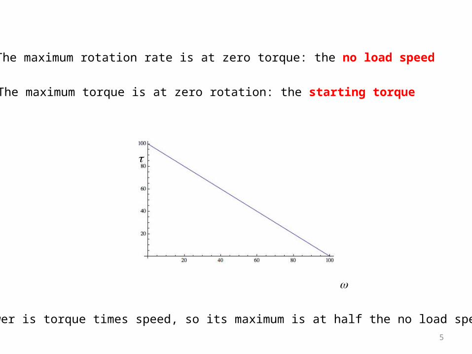
The maximum rotation rate is at zero torque: the no load speed

The maximum torque is at zero rotation: the starting torque

t

w

Power is torque times speed, so its maximum is at half the no load speed.

6

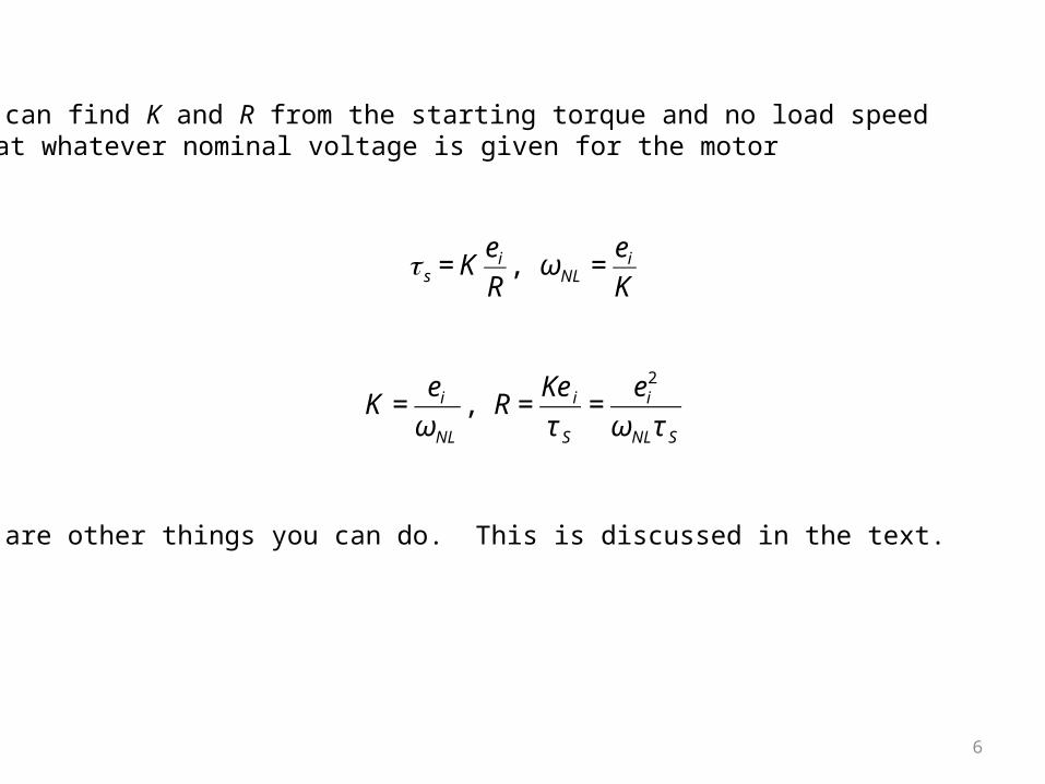
You can find K and R from the starting torque and no load speedat whatever nominal voltage is given for the motor

€

τ s = Kei

R, ωNL =

ei

K

€

K =ei

ωNL

, R =Kei

τ S

=ei

2

ωNLτ S

There are other things you can do. This is discussed in the text.

7

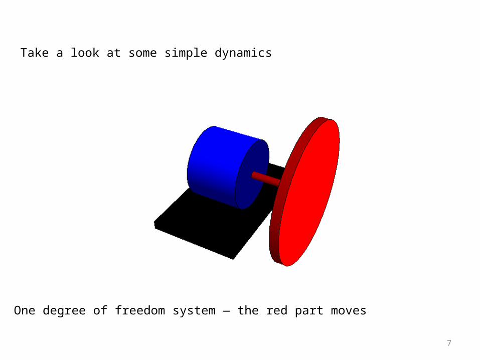
Take a look at some simple dynamics

One degree of freedom system — the red part moves

8

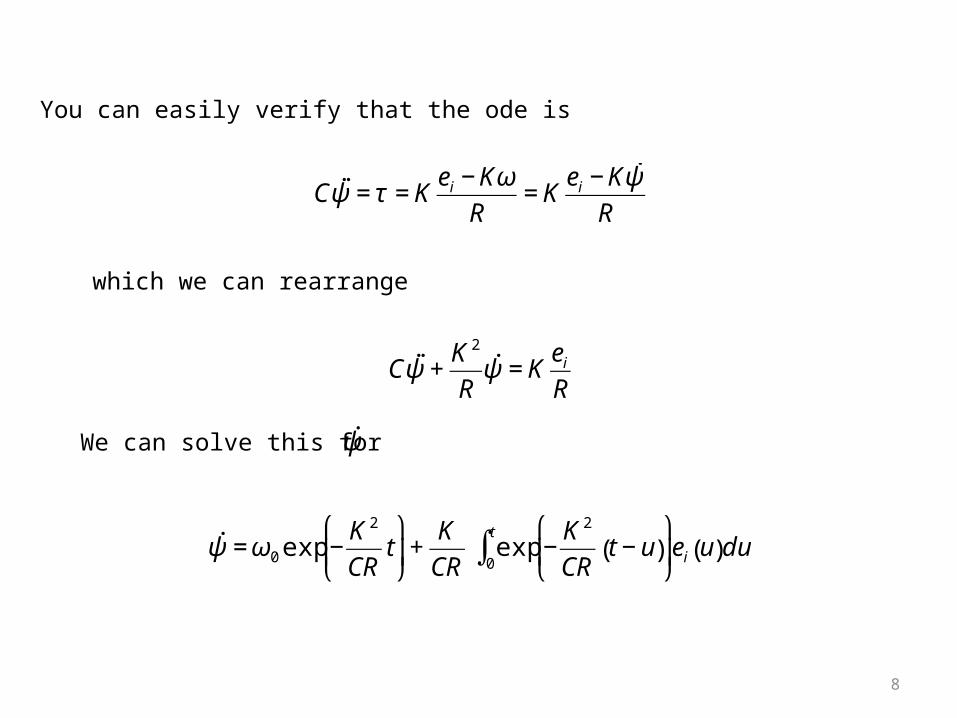
You can easily verify that the ode is

€

C ˙ ̇ ψ = τ = Kei − Kω

R= K

ei − K ˙ ψ

R

which we can rearrange

€

C ˙ ̇ ψ +K 2

R˙ ψ = K

ei

R

We can solve this for

€

˙ ψ

€

˙ ψ = ω0 exp −K 2

CRt

⎛

⎝ ⎜

⎞

⎠ ⎟+

K

CRexp −

K 2

CRt − u( )

⎛

⎝ ⎜

⎞

⎠ ⎟ei u( )du

0

t

∫

9

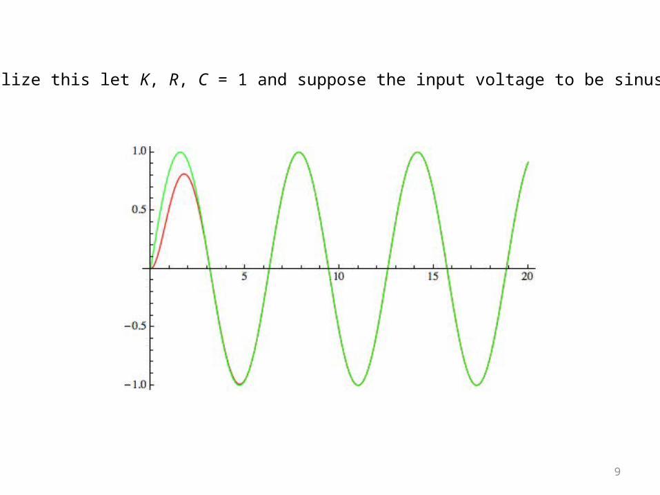
To visualize this let K, R, C = 1 and suppose the input voltage to be sinusoidal

10

Let’s look at a simple control problem: find ei to move y from 0 to π

Define a state

€

x =ψ˙ ψ

⎧ ⎨ ⎩

⎫ ⎬ ⎭=

q

u

⎧ ⎨ ⎩

⎫ ⎬ ⎭

Write the state equations, which are linear

€

˙ x =0 1

0 −K 2

CR

⎧ ⎨ ⎪

⎩ ⎪

⎫ ⎬ ⎪

⎭ ⎪x +

0K

CR

⎧ ⎨ ⎪

⎩ ⎪

⎫ ⎬ ⎪

⎭ ⎪ei

Define an error vector

€

e = x − xd( ) =ψ − π

˙ ψ

⎧ ⎨ ⎩

⎫ ⎬ ⎭

11

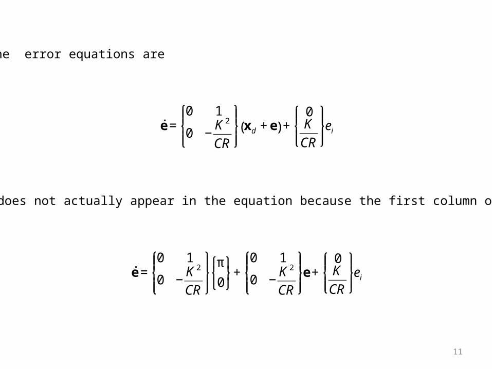
The error equations are

€

˙ e =0 1

0 −K 2

CR

⎧ ⎨ ⎪

⎩ ⎪

⎫ ⎬ ⎪

⎭ ⎪xd + e( ) +

0K

CR

⎧ ⎨ ⎪

⎩ ⎪

⎫ ⎬ ⎪

⎭ ⎪ei

The xd term does not actually appear in the equation because the first column of A is empty

€

˙ e =0 1

0 −K 2

CR

⎧ ⎨ ⎪

⎩ ⎪

⎫ ⎬ ⎪

⎭ ⎪

π

0

⎧ ⎨ ⎩

⎫ ⎬ ⎭+

0 1

0 −K 2

CR

⎧ ⎨ ⎪

⎩ ⎪

⎫ ⎬ ⎪

⎭ ⎪e +

0K

CR

⎧ ⎨ ⎪

⎩ ⎪

⎫ ⎬ ⎪

⎭ ⎪ei

12

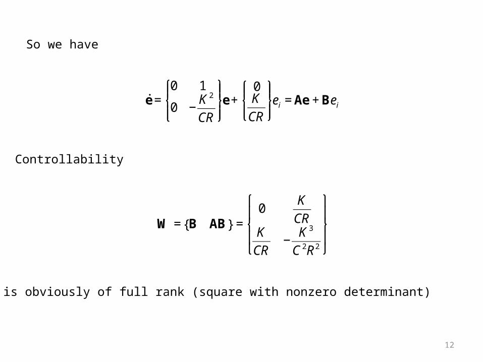
So we have

€

˙ e =0 1

0 −K 2

CR

⎧ ⎨ ⎪

⎩ ⎪

⎫ ⎬ ⎪

⎭ ⎪e +

0K

CR

⎧ ⎨ ⎪

⎩ ⎪

⎫ ⎬ ⎪

⎭ ⎪ei = Ae + Bei

Controllability

€

W = B AB{ } =0

K

CRK

CR−

K 3

C2R2

⎧

⎨ ⎪

⎩ ⎪

⎫

⎬ ⎪

⎭ ⎪

which is obviously of full rank (square with nonzero determinant)

13

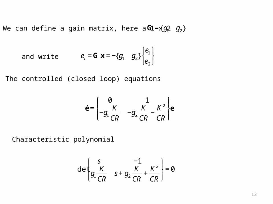
We can define a gain matrix, here a 1 x 2

€

G = g1 g2{ }

and write

€

ei = G.x = − g1 g2{ }e1

e2

⎧ ⎨ ⎩

⎫ ⎬ ⎭

The controlled (closed loop) equations

€

˙ e =0 1

−g1

K

CR−g2

K

CR−

K 2

CR

⎧ ⎨ ⎪

⎩ ⎪

⎫ ⎬ ⎪

⎭ ⎪e

Characteristic polynomial

€

dets −1

g1

K

CRs + g2

K

CR+

K 2

CR

⎧ ⎨ ⎪

⎩ ⎪

⎫ ⎬ ⎪

⎭ ⎪= 0

14

€

dets −1

g1

K

CRs + g2

K

CR+

K 2

CR

⎧ ⎨ ⎪

⎩ ⎪

⎫ ⎬ ⎪

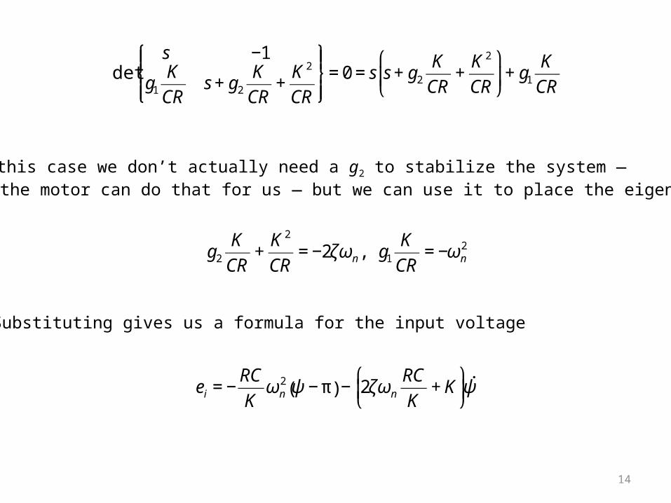
⎭ ⎪= 0 = s s + g2

K

CR+

K 2

CR

⎛

⎝ ⎜

⎞

⎠ ⎟+ g1

K

CR

In this case we don’t actually need a g2 to stabilize the system —the motor can do that for us — but we can use it to place the eigenvalues

€

g2

K

CR+

K 2

CR= −2ζωn, g1

K

CR= −ωn

2

€

ei = −RC

Kωn

2 ψ − π( ) − 2ζωn

RC

K+ K

⎛

⎝ ⎜

⎞

⎠ ⎟˙ ψ

Substituting gives us a formula for the input voltage

15

€

C ˙ ̇ ψ +K 2

R˙ ψ = K

ei

R

€

˙ ̇ ψ = −2ζωn˙ ψ −ωn

2 ψ − π( )

Combining these two equations leads us to the same input voltage

We can look at this from the nonlinear perspective, even though it it a linear problem

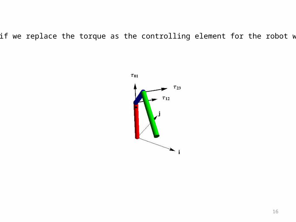
16

What happens if we replace the torque as the controlling element for the robot with voltage?

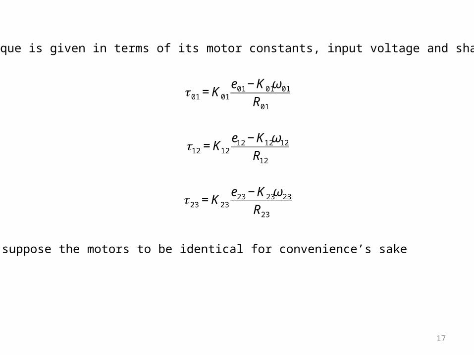
17

Each torque is given in terms of its motor constants, input voltage and shaft speed

€

τ 01 = K01

e01 − K01ω01

R01

€

τ12 = K12

e12 − K12ω12

R12

€

τ 23 = K23

e23 − K23ω23

R23

I’ll suppose the motors to be identical for convenience’s sake

18

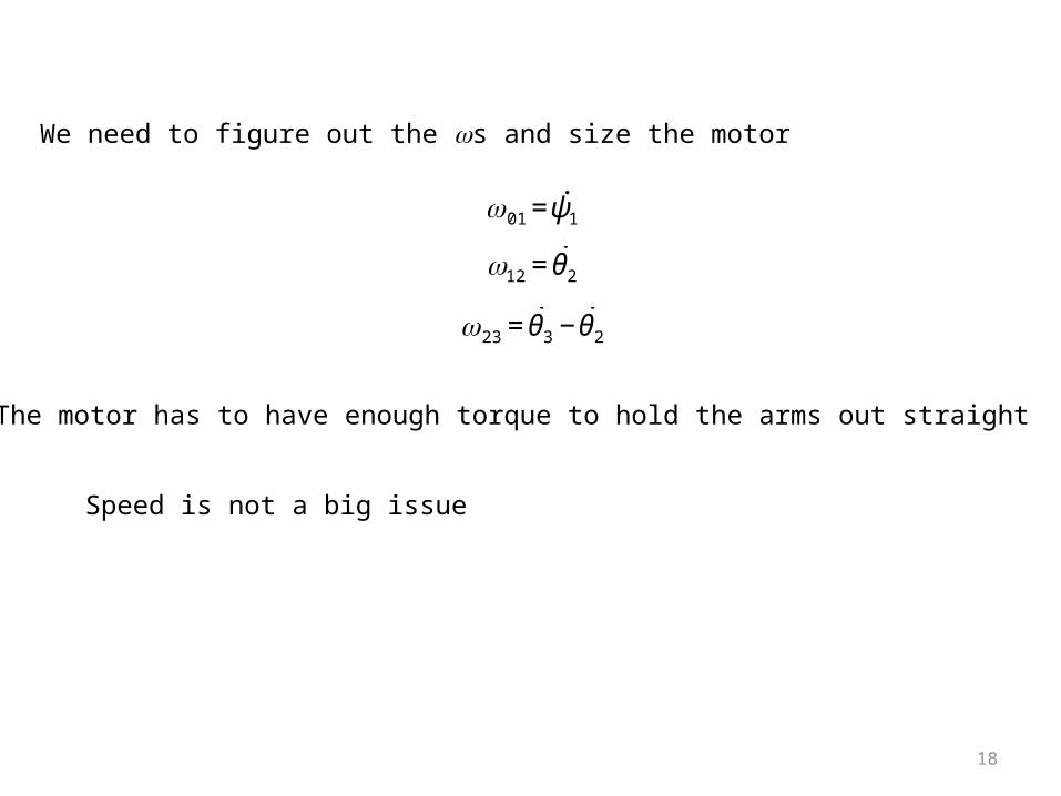
We need to figure out the ws and size the motor

€

ω01 = ˙ ψ 1

€

ω12 = ˙ θ 2

€

ω23 = ˙ θ 3 − ˙ θ 2

The motor has to have enough torque to hold the arms out straight

Speed is not a big issue

19

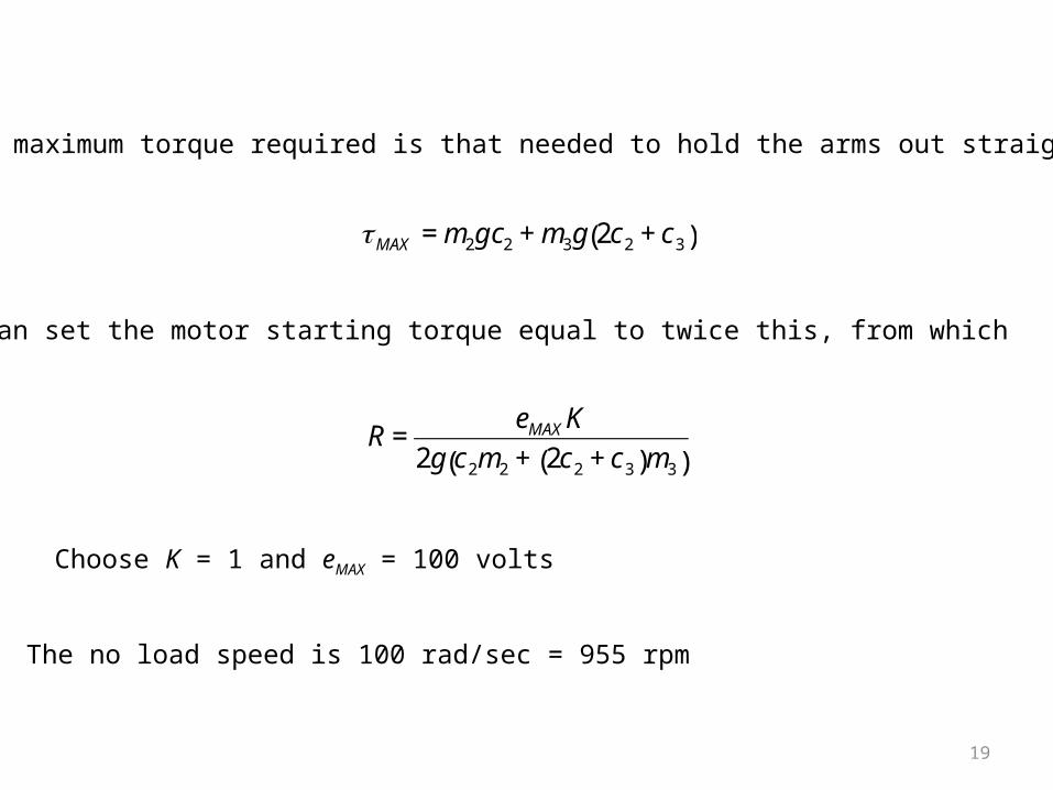
The maximum torque required is that needed to hold the arms out straight

€

τMAX = m2gc2 + m3g 2c2 + c3( )

I can set the motor starting torque equal to twice this, from which

€

R =eMAX K

2g c2m2 + 2c2 + c3( )m3( )

Choose K = 1 and eMAX = 100 volts

The no load speed is 100 rad/sec = 955 rpm

20

We can see how all this goes in Mathematica