Embed Size (px)
Citation preview
EE363 Winter 2008-09
Lecture 13
Linear quadratic Lyapunov theory
• the Lyapunov equation
• Lyapunov stability conditions
• the Lyapunov operator and integral
• evaluating quadratic integrals
• analysis of ARE
• discrete-time results
• linearization theorem
13–1
The Lyapunov equation
the Lyapunov equation is
ATP + PA + Q = 0
where A, P, Q ∈ Rn×n, and P, Q are symmetric
interpretation: for linear system x = Ax, if V (z) = zTPz, then
V (z) = (Az)TPz + zTP (Az) = −zTQz
i.e., if zTPz is the (generalized)energy, then zTQz is the associated(generalized) dissipation
linear-quadratic Lyapunov theory: linear dynamics, quadratic Lyapunovfunction
Linear quadratic Lyapunov theory 13–2
we consider system x = Ax, with λ1, . . . , λn the eigenvalues of A
if P > 0, then
• the sublevel sets are ellipsoids (and bounded)
• V (z) = zTPz = 0 ⇔ z = 0
boundedness condition: if P > 0, Q ≥ 0 then
• all trajectories of x = Ax are bounded(this means ℜλi ≤ 0, and if ℜλi = 0, then λi corresponds to a Jordanblock of size one)
• the ellipsoids {z | zTPz ≤ a} are invariant
Linear quadratic Lyapunov theory 13–3
Stability condition
if P > 0, Q > 0 then the system x = Ax is (globally asymptotically)stable, i.e., ℜλi < 0
to see this, note that
V (z) = −zTQz ≤ −λmin(Q)zTz ≤ −λmin(Q)
λmax(P )zTPz = −αV (z)
where α = λmin(Q)/λmax(P ) > 0
Linear quadratic Lyapunov theory 13–4
An extension based on observability
(Lasalle’s theorem for linear dynamics, quadratic function)
if P > 0, Q ≥ 0, and (Q,A) observable, then the system x = Ax is(globally asymptotically) stable
to see this, we first note that all eigenvalues satisfy ℜλi ≤ 0
now suppose that v 6= 0, Av = λv, ℜλ = 0
then Av = λv = −λv, so
∥
∥
∥Q1/2v
∥
∥
∥
2
= v∗Qv = −v∗(
ATP + PA)
v = λv∗Pv − λv∗Pv = 0
which implies Q1/2v = 0, so Qv = 0, contradicting observability (by PBH)
interpretation: observability condition means no trajectory can stay in the“zero dissipation” set {z | zTQz = 0}
Linear quadratic Lyapunov theory 13–5
An instability condition
if Q ≥ 0 and P 6≥ 0, then A is not stable
to see this, note that V ≤ 0, so V (x(t)) ≤ V (x(0))
since P 6≥ 0, there is a w with V (w) < 0; trajectory starting at w does notconverge to zero
in this case, the sublevel sets {z | V (z) ≤ 0} (which are unbounded) areinvariant
Linear quadratic Lyapunov theory 13–6
The Lyapunov operator
the Lyapunov operator is given by
L(P ) = ATP + PA
special case of Sylvester operator
L is nonsingular if and only if A and −A share no common eigenvalues,i.e., A does not have pair of eigenvalues which are negatives of each other
• if A is stable, Lyapunov operator is nonsingular
• if A has imaginary (nonzero, iω-axis) eigenvalue, then Lyapunovoperator is singular
thus if A is stable, for any Q there is exactly one solution P of Lyapunovequation ATP + PA + Q = 0
Linear quadratic Lyapunov theory 13–7

Solving the Lyapunov equation
ATP + PA + Q = 0
we are given A and Q and want to find P
if Lyapunov equation is solved as a set of n(n + 1)/2 equations inn(n + 1)/2 variables, cost is O(n6) operations
fast methods, that exploit the special structure of the linear equations, cansolve Lyapunov equation with cost O(n3)
based on first reducing A to Schur or upper Hessenberg form
Linear quadratic Lyapunov theory 13–8
The Lyapunov integral
if A is stable there is an explicit formula for solution of Lyapunov equation:
P =
∫
∞
0
etATQetA dt
to see this, we note that
ATP + PA =
∫
∞
0
(
ATetATQetA + etAT
QetAA)
dt
=
∫
∞
0
(
d
dtetAT
QetA
)
dt
= etATQetA
∣
∣
∣
∞
0
= −Q
Linear quadratic Lyapunov theory 13–9
Interpretation as cost-to-go
if A is stable, and P is (unique) solution of ATP + PA + Q = 0, then
V (z) = zTPz
= zT
(∫
∞
0
etATQetA dt
)
z
=
∫
∞
0
x(t)TQx(t) dt
where x = Ax, x(0) = z
thus V (z) is cost-to-go from point z (with no input) and integralquadratic cost function with matrix Q
Linear quadratic Lyapunov theory 13–10
if A is stable and Q > 0, then for each t, etATQetA > 0, so
P =
∫
∞
0
etATQetA dt > 0
meaning: if A is stable,
• we can choose any positive definite quadratic form zTQz as thedissipation, i.e., −V = zTQz
• then solve a set of linear equations to find the (unique) quadratic formV (z) = zTPz
• V will be positive definite, so it is a Lyapunov function that proves A isstable
in particular: a linear system is stable if and only if there is a quadratic
Lyapunov function that proves it
Linear quadratic Lyapunov theory 13–11
generalization: if A stable, Q ≥ 0, and (Q, A) observable, then P > 0
to see this, the Lyapunov integral shows P ≥ 0
if Pz = 0, then
0 = zTPz = zT
(∫
∞
0
etATQetA dt
)
z =
∫
∞
0
∥
∥
∥Q1/2etAz
∥
∥
∥
2
dt
so we conclude Q1/2etAz = 0 for all t ≥ 0
this implies that Qz = 0, QAz = 0, . . . , QAn−1z = 0, contradicting(Q,A) observable
Linear quadratic Lyapunov theory 13–12
Monotonicity of Lyapunov operator inverse
suppose ATPi + PiA + Qi = 0, i = 1, 2
if Q1 ≥ Q2, then for all t, etATQ1e
tA ≥ etATQ2e
tA
if A is stable, we have
P1 =
∫
∞
0
etATQ1e
tA dt ≥
∫
∞
0
etATQ2e
tA dt = P2
in other words: if A is stable then
Q1 ≥ Q2 =⇒ L−1(Q1) ≥ L−1(Q2)
i.e., inverse Lyapunov operator is monotonic, or preserves matrixinequality, when A is stable
(question: is L monotonic?)
Linear quadratic Lyapunov theory 13–13
Evaluating quadratic integrals
suppose x = Ax is stable, and define
J =
∫
∞
0
x(t)TQx(t) dt
to find J , we solve Lyapunov equation ATP + PA + Q = 0 for P
then, J = x(0)TPx(0)
in other words: we can evaluate quadratic integral exactly, by solving a setof linear equations, without even computing a matrix exponential
Linear quadratic Lyapunov theory 13–14
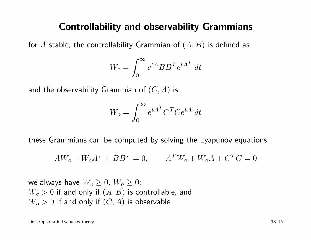
Controllability and observability Grammians
for A stable, the controllability Grammian of (A, B) is defined as
Wc =
∫
∞
0
etABBTetATdt
and the observability Grammian of (C, A) is
Wo =
∫
∞
0
etATCTCetA dt
these Grammians can be computed by solving the Lyapunov equations
AWc + WcAT + BBT = 0, ATWo + WoA + CTC = 0
we always have Wc ≥ 0, Wo ≥ 0;Wc > 0 if and only if (A, B) is controllable, andWo > 0 if and only if (C, A) is observable
Linear quadratic Lyapunov theory 13–15
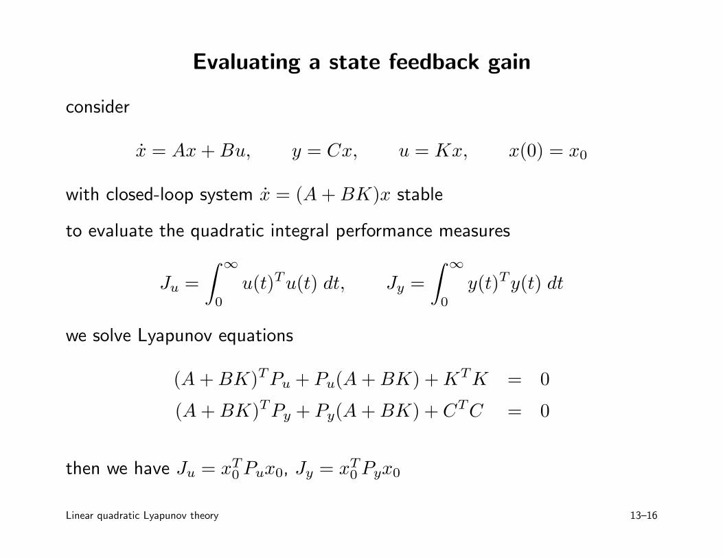
Evaluating a state feedback gain
consider
x = Ax + Bu, y = Cx, u = Kx, x(0) = x0
with closed-loop system x = (A + BK)x stable
to evaluate the quadratic integral performance measures
Ju =
∫
∞
0
u(t)Tu(t) dt, Jy =
∫
∞
0
y(t)Ty(t) dt
we solve Lyapunov equations
(A + BK)TPu + Pu(A + BK) + KTK = 0
(A + BK)TPy + Py(A + BK) + CTC = 0
then we have Ju = xT0 Pux0, Jy = xT
0 Pyx0
Linear quadratic Lyapunov theory 13–16
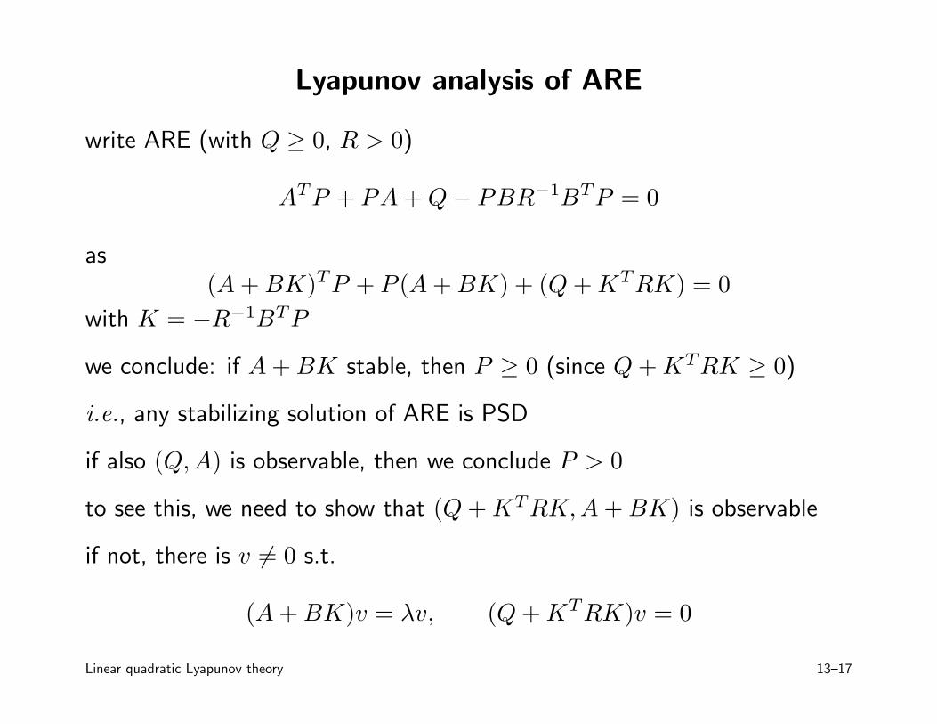
Lyapunov analysis of ARE
write ARE (with Q ≥ 0, R > 0)
ATP + PA + Q − PBR−1BTP = 0
as(A + BK)TP + P (A + BK) + (Q + KTRK) = 0
with K = −R−1BTP
we conclude: if A + BK stable, then P ≥ 0 (since Q + KTRK ≥ 0)
i.e., any stabilizing solution of ARE is PSD
if also (Q,A) is observable, then we conclude P > 0
to see this, we need to show that (Q + KTRK, A + BK) is observable
if not, there is v 6= 0 s.t.
(A + BK)v = λv, (Q + KTRK)v = 0
Linear quadratic Lyapunov theory 13–17
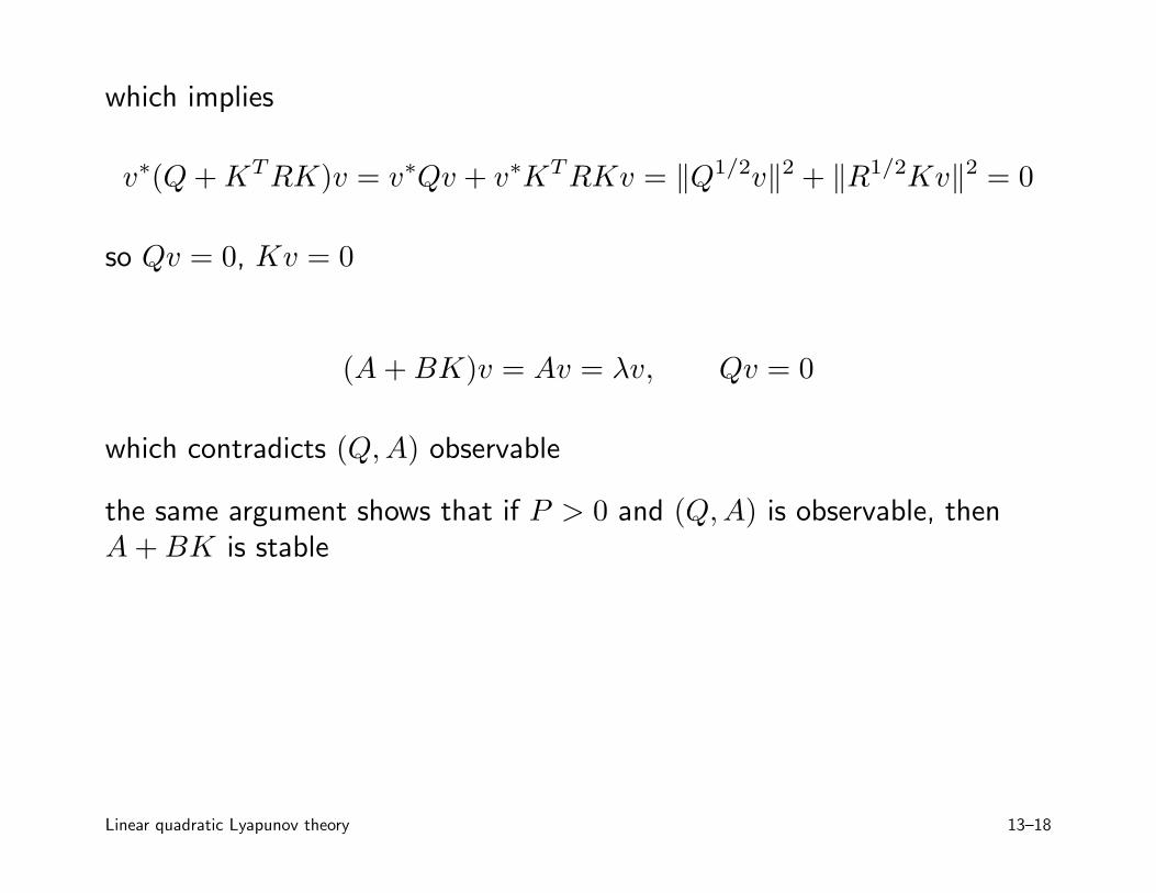
which implies
v∗(Q + KTRK)v = v∗Qv + v∗KTRKv = ‖Q1/2v‖2 + ‖R1/2Kv‖2 = 0
so Qv = 0, Kv = 0
(A + BK)v = Av = λv, Qv = 0
which contradicts (Q,A) observable
the same argument shows that if P > 0 and (Q, A) is observable, thenA + BK is stable
Linear quadratic Lyapunov theory 13–18
Monotonic norm convergence
suppose that A + AT < 0, i.e., (symmetric part of) A is negative definite
can express as ATP + PA + Q = 0, with P = I, Q > 0
meaning: xTPx = ‖x‖2 decreases along every nonzero trajectory, i.e.,
• ‖x(t)‖ is always decreasing monotonically to 0
• x(t) is always moving towards origin
this implies A is stable, but the converse is false: for a stable system, weneed not have A + AT < 0
(for a stable system with A + AT 6< 0, ‖x(t)‖ converges to zero, but notmonotonically)
Linear quadratic Lyapunov theory 13–19
for a stable system we can always change coordinates so we havemonotonic norm convergence
let P denote the solution of ATP + PA + I = 0
take T = P−1/2
in new coordinates A becomes A = T−1AT ,
A + AT = P 1/2AP−1/2 + P−1/2ATP 1/2
= P−1/2(
PA + ATP)
P−1/2
= −P−1 < 0
in new coordinates, convergence is obvious because ‖x(t)‖ is alwaysdecreasing
Linear quadratic Lyapunov theory 13–20
Discrete-time results
all linear quadratic Lyapunov results have discrete-time counterparts
the discrete-time Lyapunov equation is
ATPA − P + Q = 0
meaning: if xt+1 = Axt and V (z) = zTPz, then ∆V (z) = −zTQz
• if P > 0 and Q > 0, then A is (discrete-time) stable (i.e., |λi| < 1)
• if P > 0 and Q ≥ 0, then all trajectories are bounded(i.e., |λi| ≤ 1; |λi| = 1 only for 1 × 1 Jordan blocks)
• if P > 0, Q ≥ 0, and (Q, A) observable, then A is stable
• if P 6> 0 and Q ≥ 0, then A is not stable
Linear quadratic Lyapunov theory 13–21
Discrete-time Lyapunov operator
the discrete-time Lyapunov operator is given by L(P ) = ATPA − P
L is nonsingular if and only if, for all i, j, λiλj 6= 1(roughly speaking, if and only if A and A−1 share no eigenvalues)
if A is stable, then L is nonsingular; in fact
P =
∞∑
t=0
(AT )tQAt
is the unique solution of Lyapunov equation ATPA − P + Q = 0
the discrete-time Lyapunov equation can be solved quickly (i.e., O(n3))and can be used to evaluate infinite sums of quadratic functions, etc.
Linear quadratic Lyapunov theory 13–22
Converse theorems
suppose xt+1 = Axt is stable, ATPA − P + Q = 0
• if Q > 0 then P > 0
• if Q ≥ 0 and (Q,A) observable, then P > 0
in particular, a discrete-time linear system is stable if and only if there is aquadratic Lyapunov function that proves it
Linear quadratic Lyapunov theory 13–23
Monotonic norm convergence
suppose ATPA − P + Q = 0, with P = I and Q > 0
this means ATA < I, i.e., ‖A‖ < 1
meaning: ‖xt‖ decreases on every nonzero trajectory; indeed,‖xt+1‖ ≤ ‖A‖‖xt‖ < ‖xt‖
when ‖A‖ < 1,
• stability is obvious, since ‖xt‖ ≤ ‖A‖t‖x0‖
• system is called contractive since norm is reduced at each step
the converse is false: system can be stable without ‖A‖ < 1
Linear quadratic Lyapunov theory 13–24
now suppose A is stable, and let P satisfy ATPA − P + I = 0
take T = P−1/2
in new coordinates A becomes A = T−1AT , so
AT A = P−1/2ATPAP−1/2
= P−1/2(P − I)P−1/2
= I − P−1 < I
i.e., ‖A‖ < 1
so for a stable system, we can change coordinates so the system iscontractive
Linear quadratic Lyapunov theory 13–25
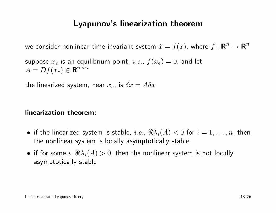
Lyapunov’s linearization theorem
we consider nonlinear time-invariant system x = f(x), where f : Rn → Rn
suppose xe is an equilibrium point, i.e., f(xe) = 0, and letA = Df(xe) ∈ Rn×n
the linearized system, near xe, is ˙δx = Aδx
linearization theorem:
• if the linearized system is stable, i.e., ℜλi(A) < 0 for i = 1, . . . , n, thenthe nonlinear system is locally asymptotically stable
• if for some i, ℜλi(A) > 0, then the nonlinear system is not locallyasymptotically stable
Linear quadratic Lyapunov theory 13–26
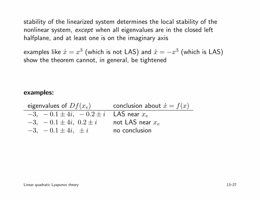
stability of the linearized system determines the local stability of thenonlinear system, except when all eigenvalues are in the closed lefthalfplane, and at least one is on the imaginary axis
examples like x = x3 (which is not LAS) and x = −x3 (which is LAS)show the theorem cannot, in general, be tightened
examples:
eigenvalues of Df(xe) conclusion about x = f(x)−3, − 0.1 ± 4i, − 0.2 ± i LAS near xe
−3, − 0.1 ± 4i, 0.2 ± i not LAS near xe
−3, − 0.1 ± 4i, ± i no conclusion
Linear quadratic Lyapunov theory 13–27
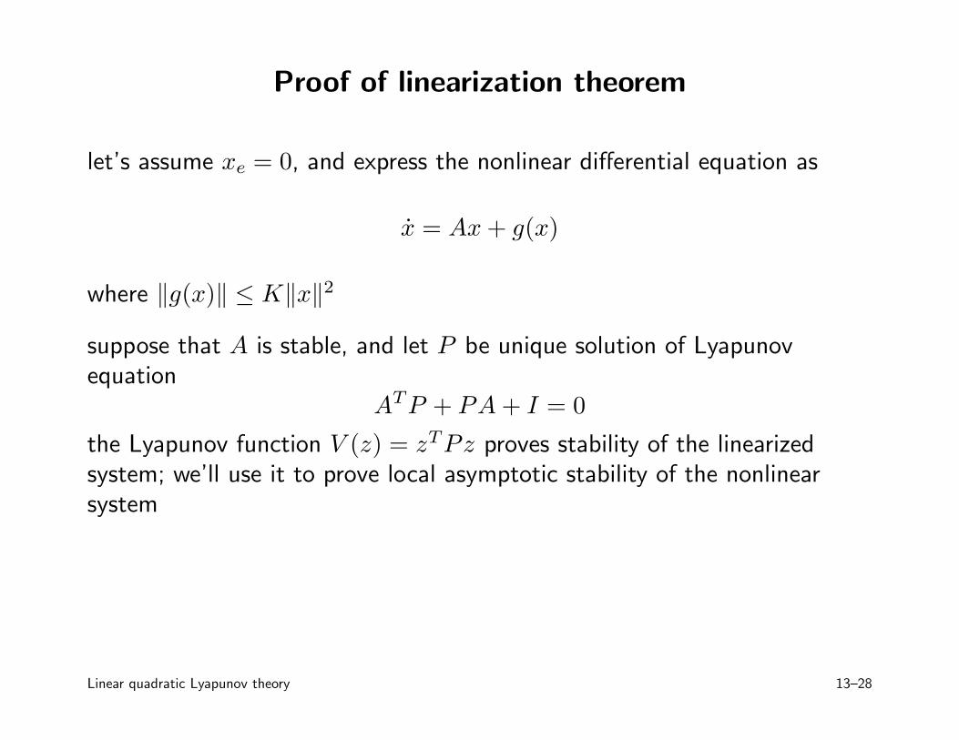
Proof of linearization theorem
let’s assume xe = 0, and express the nonlinear differential equation as
x = Ax + g(x)
where ‖g(x)‖ ≤ K‖x‖2
suppose that A is stable, and let P be unique solution of Lyapunovequation
ATP + PA + I = 0
the Lyapunov function V (z) = zTPz proves stability of the linearizedsystem; we’ll use it to prove local asymptotic stability of the nonlinearsystem
Linear quadratic Lyapunov theory 13–28
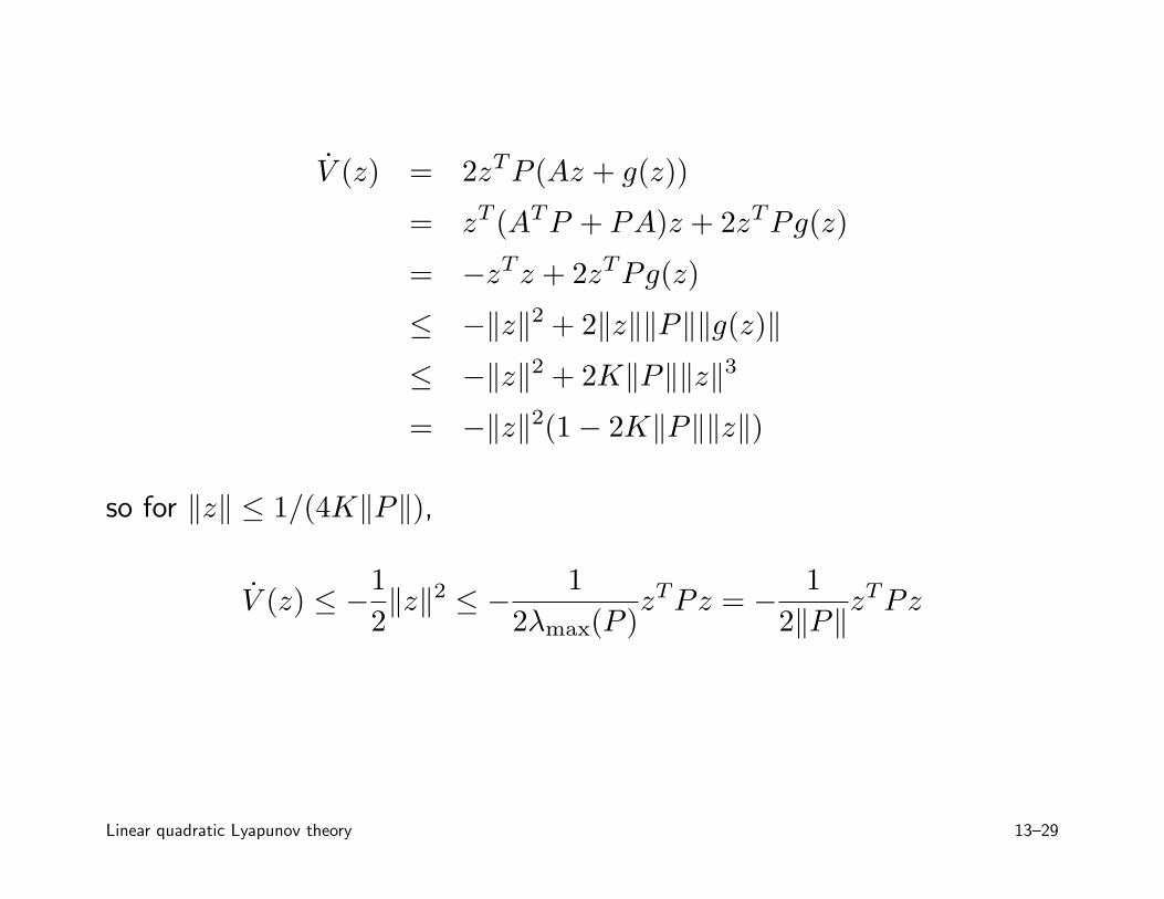
V (z) = 2zTP (Az + g(z))
= zT (ATP + PA)z + 2zTPg(z)
= −zTz + 2zTPg(z)
≤ −‖z‖2 + 2‖z‖‖P‖‖g(z)‖
≤ −‖z‖2 + 2K‖P‖‖z‖3
= −‖z‖2(1 − 2K‖P‖‖z‖)
so for ‖z‖ ≤ 1/(4K‖P‖),
V (z) ≤ −1
2‖z‖2 ≤ −
1
2λmax(P )zTPz = −
1
2‖P‖zTPz
Linear quadratic Lyapunov theory 13–29
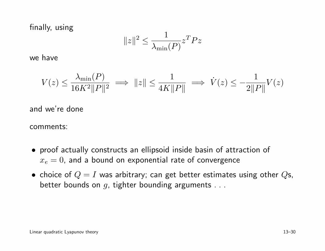
finally, using
‖z‖2 ≤1
λmin(P )zTPz
we have
V (z) ≤λmin(P )
16K2‖P‖2=⇒ ‖z‖ ≤
1
4K‖P‖=⇒ V (z) ≤ −
1
2‖P‖V (z)
and we’re done
comments:
• proof actually constructs an ellipsoid inside basin of attraction ofxe = 0, and a bound on exponential rate of convergence
• choice of Q = I was arbitrary; can get better estimates using other Qs,better bounds on g, tighter bounding arguments . . .
Linear quadratic Lyapunov theory 13–30
Integral quadratic performance
consider x = f(x), x(0) = x0
we are interested in the integral quadratic performance measure
J(x0) =
∫
∞
0
x(t)TQx(t) dt
for any fixed x0 we can find this (approximately) by simulation andnumerical integration
(we’ll assume the integral exists; we do not require Q ≥ 0)
Linear quadratic Lyapunov theory 13–31
Lyapunov bounds on integral quadratic performance
suppose there is a function V : Rn → R such that
• V (z) ≥ 0 for all z
• V (z) ≤ −zTQz for all z
then we have J(x0) ≤ V (x0), i.e., the Lyapunov function V serves as anupper bound on the integral quadratic cost
(since Q need not be PSD, we might not have V ≤ 0; so we cannotconclude that trajectories are bounded)
Linear quadratic Lyapunov theory 13–32
to show this, we note that
V (x(T )) − V (x(0)) =
∫ T
0
V (x(t)) dt ≤ −
∫ T
0
x(t)TQx(t) dt
and so
∫ T
0
x(t)TQx(t) dt ≤ V (x(0)) − V (x(T )) ≤ V (x(0))
since this holds for arbitrary T , we conclude
∫
∞
0
x(t)TQx(t) dt ≤ V (x(0))
Linear quadratic Lyapunov theory 13–33
Integral quadratic performance for linear systems
for a stable linear system, with Q ≥ 0, the Lyapunov bound is sharp, i.e.,there exists a V such that
• V (z) ≥ 0 for all z
• V (z) ≤ −zTQz for all z
and for which V (x0) = J(x0) for all x0
(take V (z) = zTPz, where P is solution of ATP + PA + Q = 0)
Linear quadratic Lyapunov theory 13–34