Lecture 13: Chapter 8, Sections 1-2 4 Stages of Statistics

(C) 2007 Nancy Pfenning

©2011 Brooks/Cole, Cengage Learning

Elementary Statistics: Looking at the Big Picture 1

Lecture 13: Chapter 8, Sections 1-2Sampling Distributions:Proportions; begin MeansoTypical Inference ProblemoDefinition of Sampling Distributiono3 Approaches to Understanding Sampling Dist.oApplying 68-95-99.7 RuleoMeans: Inference Problem, 3 ApproachesoCenter, Spread, Shape of Sample Mean

1


Elementary Statistics: Looking at the Big Picture L13.2

Looking Back: Review

o 4 Stages of Statisticsn Data Production (discussed in Lectures 1-3)n Displaying and Summarizing (Lectures 3-8)n Probability

o Finding Probabilities (discussed in Lectures 9-10)o Random Variables (discussed in Lectures 10-12)o Sampling Distributions

n Proportionsn Means

n Statistical Inference

2



Typical Inference Problem

If sample of 100 students has 0.13 left-handed,can you believe population proportion is 0.10?Solution Method: Assume (temporarily) thatpopulation proportion is 0.10, find probabilityof sample proportion as high as 0.13. If it’s tooimprobable, we won’t believe populationproportion is 0.10.

3



Key to Solving Inference Problems

For a given population proportion p and sample size n, need to find probability of sample proportion in a certain range:

Need to know sampling distribution of .Note: can denote a single statistic or a

random variable.

4




Definition

Sampling distribution of sample statistic tells probability distribution of values taken by the statistic in repeated random samples of a given size.

Looking Back: We summarize a probability distribution by reporting its center, spread, shape.

5



Behavior of Sample Proportion (Review)

For random sample of size n from population with p in category of interest, sample proportion has

n mean pn standard deviationn shape approximately normal for large

enough n Looking Back: Can find normal probabilities using 68-95-99.7 Rule, etc.

6



Rules of Thumb (Review)

n Population at least 10 times sample size n(formula for standard deviation of approximately correct even if sampled without replacement)

n np and n(1-p) both at least 10(guarantees approximately normal)

7



Understanding Dist. of Sample Proportion

3 Approaches:1. Intuition2. Hands-on Experimentation3. Theoretical Results

Looking Ahead: We’ll find that our intuition is consistent with experimental results, and both are confirmed by mathematical theory.

8




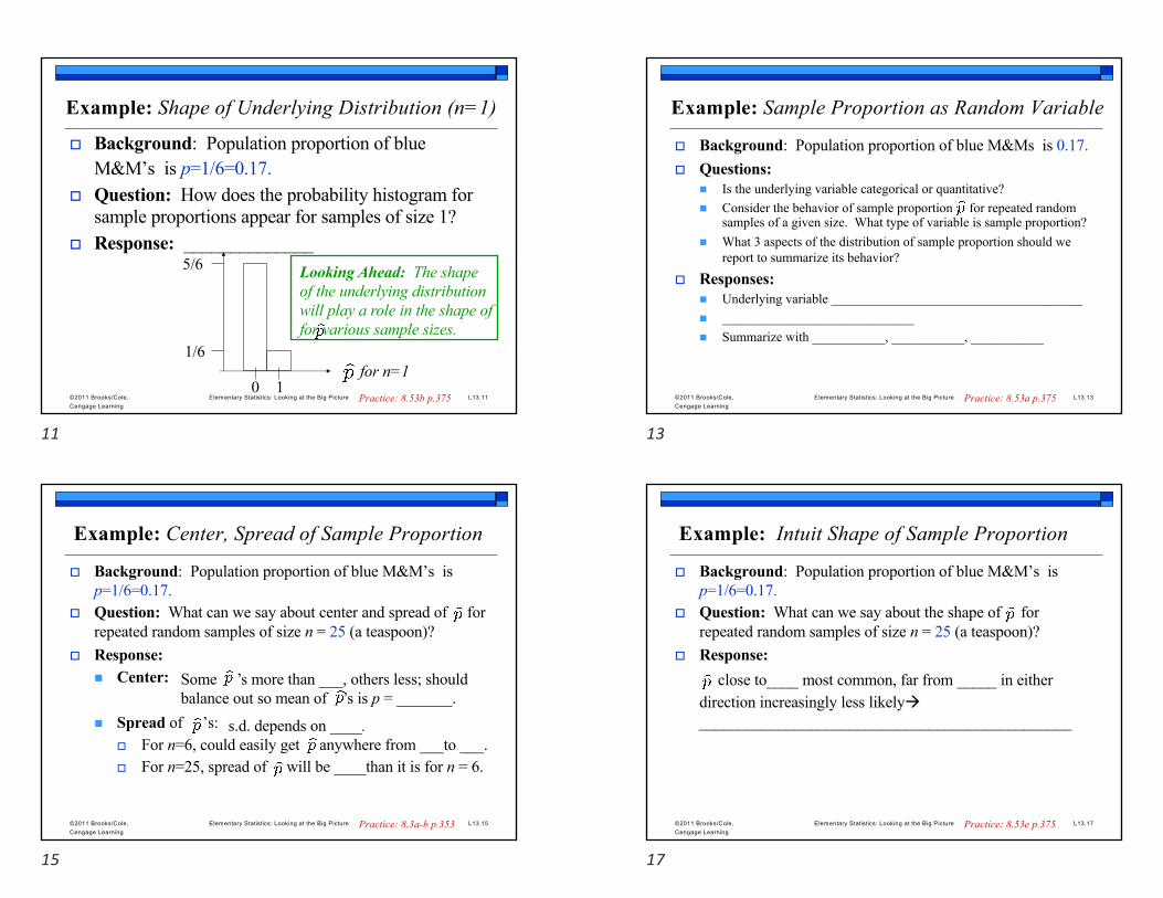
Example: Shape of Underlying Distribution (n=1)

o Background: Population proportion of blue M&M’s is p=1/6=0.17.

o Question: How does the probability histogram for sample proportions appear for samples of size 1?

o Response: ______________

for n=1

5/6

1/6

0 1

Looking Ahead: The shape of the underlying distribution will play a role in the shape of for various sample sizes.

Practice: 8.53b p.375

11



Example: Sample Proportion as Random Variable

o Background: Population proportion of blue M&Ms is 0.17. o Questions:

n Is the underlying variable categorical or quantitative?n Consider the behavior of sample proportion for repeated random

samples of a given size. What type of variable is sample proportion?n What 3 aspects of the distribution of sample proportion should we

report to summarize its behavior?

o Responses: n Underlying variable ______________________________________n _____________________________n Summarize with ___________, ___________, ___________

Practice: 8.53a p.375

13



Example: Center, Spread of Sample Proportion


o Question: What can we say about center and spread of for repeated random samples of size n = 25 (a teaspoon)?

o Response: n Center:

n Spread of ’s: o For n=6, could easily get anywhere from ___to ___.o For n=25, spread of will be ____than it is for n = 6.

Some ’s more than ___, others less; should balance out so mean of ’s is p = _______.

s.d. depends on ____.

Practice: 8.3a-b p.353

15



Example: Intuit Shape of Sample Proportion


o Question: What can we say about the shape of for repeated random samples of size n = 25 (a teaspoon)?

o Response: close to____ most common, far from _____ in either

direction increasingly less likelyà_______________________________________________

Practice: 8.53e p.375

17




Example: Sample Proportion for Larger n


o Question: What can we say about center, spread, shape of for repeated random samples of size n = 75 (a Tablespoon)?

o Response: n Center:n Spread of ’s: compared to n=25, spread for n=75 is ____n Shape: ’s clumped near 0.17, taper at tailsà _________

mean of ’s should be p = _____ (for any n).

Looking Ahead: Sample size does not affect center but plays an important role in spread and shape of the distribution of sample proportion (also of sample mean).

Practice: 8.5 p.354

19



Understanding Sample Proportion



20



Central Limit Theorem

Approximate normality of sample statistic for repeated random samples of a large enough size is cornerstone of inference theory.

o Makes intuitive sense.o Can be verified with experimentation.o Proof requires higher-level mathematics;

result called Central Limit Theorem.

21



Center of Sample Proportion (Implications)


n mean pà is unbiased estimator of p

(sample must be random)

22




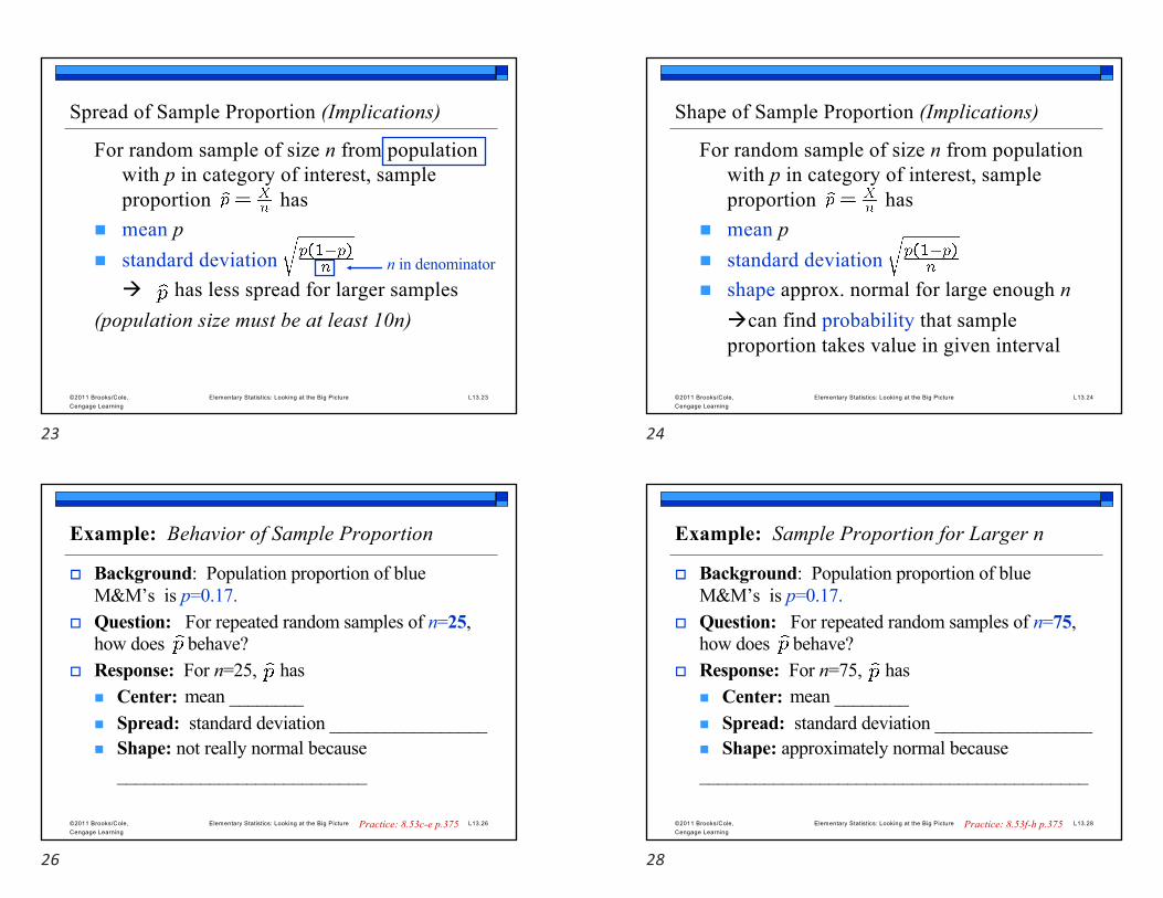
Spread of Sample Proportion (Implications)


n mean pn standard deviation

à has less spread for larger samples(population size must be at least 10n)

n in denominator

23



Shape of Sample Proportion (Implications)


n mean pn standard deviationn shape approx. normal for large enough n

àcan find probability that sample proportion takes value in given interval

24



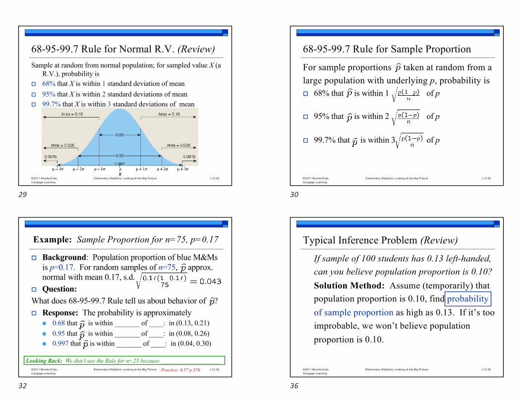
Example: Behavior of Sample Proportion

o Background: Population proportion of blue M&M’s is p=0.17.

o Question: For repeated random samples of n=25, how does behave?

o Response: For n=25, has n Center:n Spread: standard deviation _________________n Shape: not really normal because

___________________________

mean ________

Practice: 8.53c-e p.375

26



Example: Sample Proportion for Larger n

o Background: Population proportion of blue M&M’s is p=0.17.

o Question: For repeated random samples of n=75, how does behave?

o Response: For n=75, has n Center:n Spread: standard deviation _________________n Shape: approximately normal because __________________________________________

mean ________

Practice: 8.53f-h p.375

28




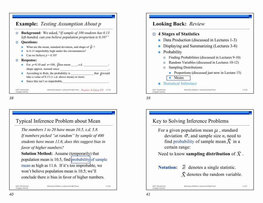
68-95-99.7 Rule for Normal R.V. (Review)Sample at random from normal population; for sampled value X (a

R.V.), probability iso 68% that X is within 1 standard deviation of meano 95% that X is within 2 standard deviations of meano 99.7% that X is within 3 standard deviations of mean

29



68-95-99.7 Rule for Sample Proportion

For sample proportions taken at random from alarge population with underlying p, probability iso 68% that is within 1 of p

o 95% that is within 2 of p

o 99.7% that is within 3 of p

30



Example: Sample Proportion for n=75, p=0.17

o Background: Population proportion of blue M&Ms is p=0.17. For random samples of n=75, approx. normal with mean 0.17, s.d.

o Question: What does 68-95-99.7 Rule tell us about behavior of ?o Response: The probability is approximately

n 0.68 that is within _______ of ____: in (0.13, 0.21)n 0.95 that is within _______ of ____: in (0.08, 0.26)n 0.997 that is within _______ of ____: in (0.04, 0.30)

Looking Back: We don’t use the Rule for n=25 because ____________________Practice: 8.57 p.376

32



Typical Inference Problem (Review)

If sample of 100 students has 0.13 left-handed,can you believe population proportion is 0.10?Solution Method: Assume (temporarily) thatpopulation proportion is 0.10, find probabilityof sample proportion as high as 0.13. If it’s tooimprobable, we won’t believe populationproportion is 0.10.

36




Example: Testing Assumption About p o Background: We asked, “If sample of 100 students has 0.13

left-handed, can you believe population proportion is 0.10?”o Questions:

n What are the mean, standard deviation, and shape of ? n Is 0.13 improbably high under the circumstances?n Can we believe p = 0.10?

o Response:n For p=0.10 and n=100, has mean ____, s.d. ________________ ;

shape approx. normal since _________________________________.n According to Rule, the probability is _______________ that would

take a value of 0.13 (1 s.d. above mean) or more. n Since this isn’t so improbable, ______________________________.

Practice: 8.11d-f p.355

38



Looking Back: Review

o 4 Stages of Statisticsn Data Production (discussed in Lectures 1-3)n Displaying and Summarizing (Lectures 3-8)n Probability

o Finding Probabilities (discussed in Lectures 9-10)o Random Variables (discussed in Lectures 10-12)o Sampling Distributions

n Proportions (discussed just now in Lecture 13)n Means

n Statistical Inference

39



Typical Inference Problem about MeanThe numbers 1 to 20 have mean 10.5, s.d. 5.8.If numbers picked “at random” by sample of 400students have mean 11.6, does this suggest bias infavor of higher numbers?Solution Method: Assume (temporarily) thatpopulation mean is 10.5, find probability of samplemean as high as 11.6. If it’s too improbable, wewon’t believe population mean is 10.5; we’llconclude there is bias in favor of higher numbers.

40



Key to Solving Inference Problems

For a given population mean , standard deviation , and sample size n, need to find probability of sample mean in a certain range:

Need to know sampling distribution of .

Notation: denotes a single statistic.denotes the random variable.

41




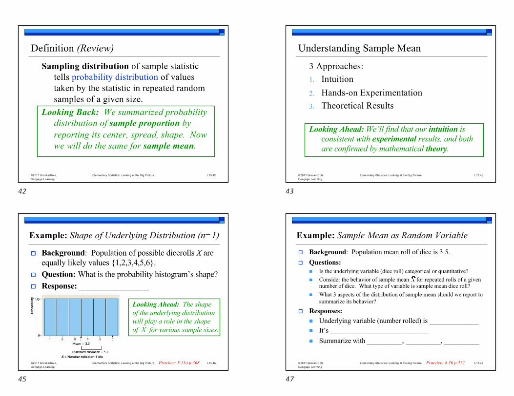
Definition (Review)

Sampling distribution of sample statistic tells probability distribution of values taken by the statistic in repeated random samples of a given size.

Looking Back: We summarized probability distribution of sample proportion by reporting its center, spread, shape. Now we will do the same for sample mean.

42



Understanding Sample Mean



43



Example: Shape of Underlying Distribution (n=1)

o Background: Population of possible dicerolls X are equally likely values {1,2,3,4,5,6}.

o Question: What is the probability histogram’s shape?o Response: _________________

Looking Ahead: The shape of the underlying distribution will play a role in the shape of X for various sample sizes.

Practice: 8.25a p.368

45



Example: Sample Mean as Random Variable

o Background: Population mean roll of dice is 3.5.o Questions:

n Is the underlying variable (dice roll) categorical or quantitative?n Consider the behavior of sample mean for repeated rolls of a given

number of dice. What type of variable is sample mean dice roll?n What 3 aspects of the distribution of sample mean should we report to

summarize its behavior?

o Responses: n Underlying variable (number rolled) is ______________n It’s ____________________________n Summarize with __________, __________, __________

Practice: 8.36 p.372

47




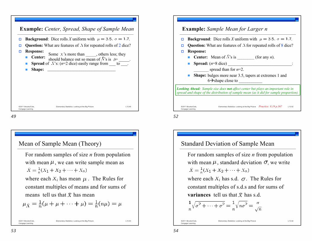
Example: Center, Spread, Shape of Sample Mean

o Background: Dice rolls X uniform with . o Question: What are features of for repeated rolls of 2 dice?o Response:

n Center:n Spread of ’s: (n=2 dice) easily range from ___ to ___.n Shape:

Some ’s more than _____, others less; they should balance out so mean of ’s is = _____.

________________________________

49



Example: Sample Mean for Larger n

o Background: Dice rolls X uniform with . o Question: What are features of for repeated rolls of 8 dice?o Response:

n Center:n Spread: (n=8 dice) ______________________________:

_______ spread than for n=2.n Shape:

Mean of ’s is ________ (for any n).

bulges more near 3.5, tapers at extremes 1 and 6àshape close to ___________

Looking Ahead: Sample size does not affect center but plays an important role in spread and shape of the distribution of sample mean (as it did for sample proportion).

Practice: 8.19 p.367

52



Mean of Sample Mean (Theory)

For random samples of size n from population with mean , we can write sample mean as

where each has mean . The Rules forconstant multiples of means and for sums ofmeans tell us that has mean

53



Standard Deviation of Sample Mean

For random samples of size n from population with mean , standard deviation , we write

where each has s.d. . The Rules forconstant multiples of s.d.s and for sums ofvariances tell us that has s.d.

54




Rule of Thumb (Review)

n Need population size at least 10n(formula for s.d. of approx. correct even if sampled without replacement)

Note: For means, there is no Rule of Thumb for approximate normality that is as simple as the one for proportions [np and n(1-p) both at least 10].

55



Central Limit Theorem (Review)

Approximate normality of sample statistic for repeated random samples of a large enough size is cornerstone of inference theory.

o Makes intuitive sense.o Can be verified with experimentation.o Proof requires higher-level mathematics;

result called Central Limit Theorem.

56



Shape of Sample Mean

For random samples of size n from population of quantitative values X, the shape of the distribution of sample mean is approximately normal if

n X itself is normal; orn X is fairly symmetric and n is at least 15; orn X is moderately skewed and n is at least 30

57



Behavior of Sample Mean: Summary

For random sample of size n from population with mean , standard deviation , sample mean has

n meann standard deviationn shape approximately normal for large

enough n

58




Center of Sample Mean (Implications)

For random sample of size n from population with mean , sample mean has

n meanà is unbiased estimator of

(sample must be random)

Looking Ahead: We’ll rely heavily on this result when we perform inference. As long as the sample is random, sample mean is our “best guess” for unknown population mean.

59



Spread of Sample Mean (Implications)

For random sample of size n from population with mean , s.d. , sample mean has

n meann standard deviation à has less spread for larger samples(population size must be at least 10n)

n in denominator

Looking Ahead: This result also impacts inference conclusions to come. Sample mean from a larger sample gives us a better estimate for the unknown population mean.

60



Shape of Sample Mean (Implications)For random sample of size n from population

with mean , s.d. , sample mean hasn meann standard deviation n shape approx. normal for large enough n

àcan find probability that sample mean takes value in given interval

Looking Ahead: Finding probabilities about sample mean will enable us to solve inference problems.

61



Example: Behavior of Sample Mean, 2 Dice

o Background: Population of dice rolls has

o Question: For repeated random samples of n=2, how does sample mean behave?

o Response: For n=2, sample mean roll hasn Center: mean _________ n Spread: standard deviation ________________n Shape: _________ because the population is flat,

not normal, and _______________Practice: 8.75a p.381

63




Example: Behavior of Sample Mean, 8 Dice

o Background: Population of dice rolls has

o Question: For repeated random samples of n=8, how does sample mean behave?

o Response: For n=8, sample mean roll hasn Center: mean __________ n Spread: standard deviation ________________n Shape: _______ normal than for n=2

(Central Limit Theorem)Practice: 8.15 p.366

65



Lecture Summary(Distribution of Sample Proportion)

o Typical inference problemo Sampling distribution; definitiono 3 approaches to understanding sampling dist.

n Intuitionn Hands-on experimentn Theory

o Center, spread, shape of sampling distributionn Central Limit Theorem

o Role of sample sizeo Applying 68-95-99.7 Rule

66



Lecture Summary(Sampling Distributions; Means)o Typical inference problem for meanso 3 approaches to understanding dist. of sample

meann Intuitn Hands-onn Theory

o Center, spread, shape of dist. of sample mean

67

Documents

Lecture 13: Chapter 8, Sections 1-2 4 Stages of Statistics