Lecture 12 –Matrix Models for Population Biologygrandjb/wildpop/lectures/lect_12.pdf · The age-structured transition matrix model representing this system ... Life cycle graph

1 of 23

WILD 7250 - Analysis of Wildlife Populations www.auburn.edu/~grandjb/wildpop

Lecture 12 –Matrix Models for Population Biology Resources:

Caswell, H. 2001. Matrix population models. 2nd ed. Sinauer Associates, Inc. Sunderland, Mass.

Manley, B.F.J. 1990. Stage-structured population: sampling, analysis, and simulation. Chapman and Hall, New York.

Matrix Arithmetic

1. Addition and subtraction

Simply addition (subtraction) of the corresponding elements in the matrices. Matrices must be of the same rank (dimension).

⎥⎥⎥⎥

⎦

⎤

⎢⎢⎢⎢

⎣

⎡

−−−−−−−−−

=−

⎥⎥⎥⎥

⎦

⎤

⎢⎢⎢⎢

⎣

⎡

−−−−

−

=+

⎥⎥⎥⎥

⎦

⎤

⎢⎢⎢⎢

⎣

⎡

−−−

−=

⎥⎥⎥⎥

⎦

⎤

⎢⎢⎢⎢

⎣

⎡

−−−

−−

=

1710736443444111

59325344

056010113

28116314

21527012

312110502412

3101

BA

BA

B

A

2. Multiplication

For the matrices A, B, and C with corresponding elements aij , bij., and cij., where C is the product of AxB. The element cij is the sum of the j products of the elements of row i of matrix A and the elements of column i of B. Note that matrices must have the same “inner” dimension. Matrix dimensions are specified as rows x columns. Thus a 4x3 matrix can be multiplied by a 3x1 matrix, but the order of the multiplication can not be reversed (i.e., a 1x3 matrix cannot be multiplied by a 4x3 matrix).

lect_12.doc

2 of 23


lect_12.doc

⎥⎢

⎥⎥

⎢⎢=⎥

⎥⎢⎢ +++−=× 11184521624BA

⎥⎥⎥

⎦

⎤

⎢⎢⎢

⎣

⎡

−

−=

⎥⎥⎥

⎦

⎤

⎢⎢⎢

⎣

⎡×

⎥⎥⎥

⎦

⎤

⎢⎢⎢

⎣

⎡

−

−=

050412101

100010001

050412101

* IA

⎥⎥⎥⎥⎥⎤

⎢⎢⎢⎢⎢⎡

=×

⎥⎥⎥

⎦

⎤

⎢⎢⎢

⎣

⎡=

⎥⎥⎥

⎦

⎤

⎢⎢⎢

⎣

⎡=

∑∑∑∑∑∑

jjjj

jjj

jjj

jjj

jjj

baba

baba

baba

BA

bbbbbb

Baaaaaaaaa

A

2313

2212

2111

3231

2221

1211

333231

232221

131211

⎦⎣ jj

⎤⎡−⎤⎡ −+−+

⎥⎥⎥

⎦

⎤

⎢⎢⎢

⎣

⎡−=

⎥⎥⎥

⎦

⎤

⎢⎢⎢

⎣

⎡

−

−=

02101402

145212

050412101

BA

Example:

⎥⎦⎢⎣ −⎥⎦⎢⎣ +−++ 251002500100

⎥⎥⎥

⎦

⎤

⎢⎢⎢

⎣

⎡=

⎥⎥⎥

⎦

⎤

⎢⎢⎢

⎣

⎡

−

−=

100010001

050412101

IA

The identity matrix. For any square matrix, the identity is a diagonal matrix of equal rank with all of the diagonal elements = 1.

Leslie and Lefkovitch Projection Matrices

1. History

• Application of age-specific survival and fertility rates dates back to the late 19th century

• Use of matrix models was developed independently by Bernardelli (1941), Lewis (1942), and Leslie (1945).

• Bernardelli’s 1941 paper in the Journal of the Burma Research Society focused on oscillations in the age structure of the Burmese population from 1901-1931.

3 of 23


• Lewis suggested age-structured matrix models in a 1942 paper, appearing in the Indian Journal of Statistics, that was very similar to Leslie’s 1945 paper.

• Leslie’s works published in 1945, 1948, 1959, and 1966 were apparently the most influential.

• 1945 – age-specific projection equations in matrix form, rates of increase, and stable age distributions.

• 1948 – examined relationships to logistic models and predator-prey interactions.

• 1959 – effects of time-lags on matrix models.

• 1966 – intrinsic rates of increase and overlap in generations on guillemots populations

• Even so matrix models were not mentioned in many notable ecology texts or in ecological research prior to the 1970s.

• Lefkovitch worked on the dynamics of agricultural pests published a series of influential papers using the matrix models described by Leslie in the early 1960s. Among these was a 1965 paper that introduced the idea of stage-structured models that classified insects by life-stage rather than age. This idea was rapidly adopted by ecologists classifying trees by size, humans by age-groups, and various plants by life-stage and size.

• Before the advent of small computers, much of the work by Leslie and others focused on the parallels with life tables and transformations to make matrix calculations easier (by hand).

2. Age-structured models

The goal of population modeling is to develop equations that allow us to understand the processes that govern population dynamics. Consider the equation:

lect_12.doc

tt NN = λ+

tt NPFN )(1

1 ,

where Nt is the population size in year t and Nt+1. In the absence of emigration and immigration, the population growth rate, λ, subsumes the processes of mortality and recruitment. Thus, one could more explicitly write this equation as

= ++ ,

where F is fertility, the number of offspring recruited per adult and P is the probability of surviving from year t until year t+1.

Now consider a population of size N with 3 1-year age classes where ni is the number of individuals in age-class i and age class one is the youngest age class. The dynamics of this population could be expressed as three separate equations:

4 of 23


1112

313221111

nPn

nFnFnFn

t

tttt

=

++=

lect_12.doc

2213 nPn t =+

⎥⎥⎥

⎦

⎤

⎢⎢⎡

=0001

321

PFFF

A

⎥⎥⎥

⎦

⎤

⎢⎢⎢

⎣

⎡×

⎥⎥⎥

⎦

⎤

⎢⎢⎢

⎣

⎡=

+

+

,

and since individuals in this population do not live beyond age 3, all of the n3s die before the next time step (year). Note that n1 t+1 is composed of offspring produced by all three age classes, and that n2 t+1 and n3 t+1 contain only individuals from n1 t and n2 t (respectively) that survived until t+1.

The age-structured transition matrix model representing this system of equations is a square matrix with one column for each age-class:

⎢⎣ 0 2P

The population N, composed of individuals of three age classes n1-3 is represented by the vector:

⎥⎥⎥

⎦

⎤

⎢⎢⎢

⎣

⎡=

3

2

1

nnn

N .

This population is projected through time using matrix multiplication by the equation:

= ×+

3

2

1

2

1

321

1

0000

nnn

PP

FFFNAN tt

.

(Note that the inner dimensions of the matrices (3x3;3x1) agree.)

This model can be represented by the above life-cycle diagram, where each node represents an age class, the straight lines connecting the nodes represent the survival

1 2 3

5 of 23


lect_12.doc

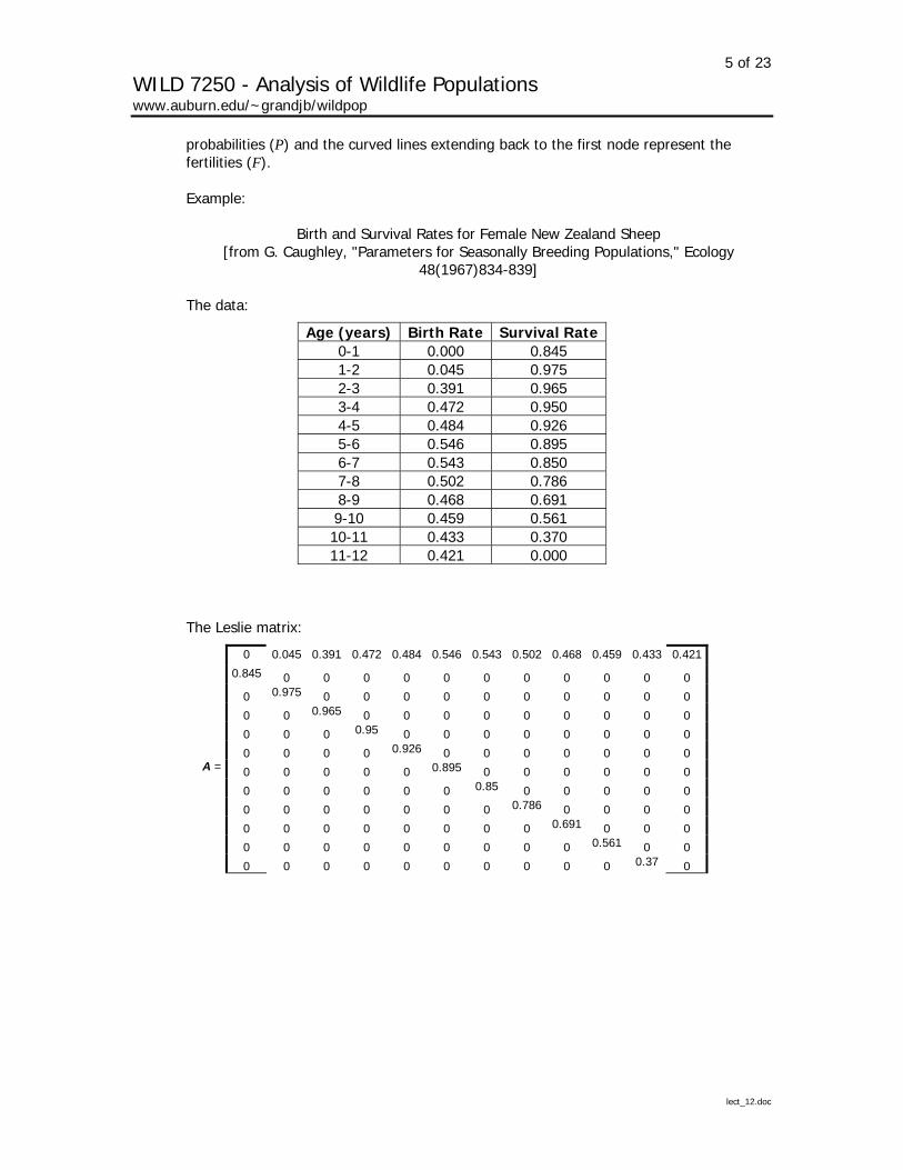
probabilities (P) and the curved lines extending back to the first node represent the fertilities (F).

Example:

Birth and Survival Rates for Female New Zealand Sheep [from G. Caughley, "Parameters for Seasonally Breeding Populations," Ecology

48(1967)834-839]

The data:

Age (years) Birth Rate Survival Rate0-1 0.000 0.845 1-2 0.045 0.975 2-3 0.391 0.965 3-4 0.472 0.950 4-5 0.484 0.926 5-6 0.546 0.895 6-7 0.543 0.850 7-8 0.502 0.786 8-9 0.468 0.691 9-10 0.459 0.561 10-11 0.433 0.370 11-12 0.421 0.000

The Leslie matrix:

0 0.045 0.391 0.472 0.484 0.546 0.543 0.502 0.468 0.459 0.433 0.421

0.845 0 0 0 0 0 0 0 0 0 0 0 0 0.975 0 0 0 0 0 0 0 0 0 0 0 0 0.965 0 0 0 0 0 0 0 0 0 0 0 0 0.95 0 0 0 0 0 0 0 0 0 0 0 0 0.926 0 0 0 0 0 0 0

A = 0 0 0 0 0 0.895 0 0 0 0 0 0 0 0 0 0 0 0 0.85 0 0 0 0 0 0 0 0 0 0 0 0 0.786 0 0 0 0 0 0 0 0 0 0 0 0 0.691 0 0 0 0 0 0 0 0 0 0 0 0 0.561 0 0 0 0 0 0 0 0 0 0 0 0 0.37 0

6 of 23


Life-cycle diagram:

1 2 3 4 5 6 7 8 9 10

11

12

1 2 3 4 5 6 7 8 9 10

11

12

10-year projection starting with 100 2-year olds:

Note the rapidly (exponential) increasing population and the initial fluctuations in λ due to starting conditions (age distribution).

Age distributions - 10-year projection starting with 100 2-year olds.

lect_12.doc

0

100

200

300

400

500

600

0 1 2 3 4 5 6 7 8 9 10Year

N

Stage 12

Stage 11

Stage 10

Stage 9

Stage 8

Stage 7

Stage 6

Stage 5

Stage 4

Stage 3

Stage 2

Stage 1

0

100

200

300

400

500

600

0 1 2 3 4 5 6 7 8 9 10

Year

N

0.9

1

1.1

1.2

1.3

1.4

N λ

7 of 23


3. Assumptions of age structured models: a. Individuals progress through the life-cycle by discrete time-steps (e.g., years) b. Age-specific fertility c. Age-specific survival

4. Stage-based models

The works of Lefkovitch relaxed the assumptions of the age-structured models described by Leslie and were useful for animals that had stage-dependent vital rates.

1) Discrete time-steps (e.g., years)

2) Individuals allowed to remain in life-stages longer than one year

3) Stage-specific fertility

4) Stage-specific survival

lect_12.doc

⎥⎥⎥

⎦

⎤

⎢⎢⎢

⎣

⎡=

32

21

321

00PG

PGFFP

A

Stage-based matrix model (3 stages):

F i is still the fertility, the number of offspring recruited per adult; Pi is the probability of surviving from year t until year t+1 and remaining in stage i ; and Gi is the probability of growing to stage i during the next time step.

Life cycle graph for a typical 4-stage population:

1 2 3 4G1

P2 P3 P4P1

G3G2

F3

F4

F2

Examples:

1) Arthropods with discrete developmental stages.

2) Plants, crustaceans, and fish with size-dependent ages of maturity.

8 of 23


3) Angiosperms, kelp, molluscs, decapods, insects, isopods, amphibians, and reptiles with reproductive rates that vary with adult body size.

4) Plants with mortality rates that vary with size.

5) Plants and animals with size related sex changes.

Another example – from Brault, S. and Caswell, H. 1973. Pod-Specific Demography of Killer Whales (Orcinus orca). Ecology, 74:1444-1454.

Classified the population into 4 stages of females: yearlings (1 year olds), juveniles (up to 18 yrs), reproductive (up to 45 yrs), and post-reproductive. Thus the life-cycle graph

looks like:

1 2 3 4G1

P2 P3 P4

G3G2

F3F2

1 2 3 4G1

P2 P3 P4

G3G2

F3F2

0.000 0.004 0.113 0.0000.978 0.911 0.000 0.0000.000 0.074 0.953 0.000

A =

0.000 0.000 0.045 0.980

Projections:

0

20

40

60

80

100

120

0 10 20 30 40 50

Year

N

Stage 1Stage 2Stage 3Stage 4

0

50

100

150

200

250

300

350

400

0 5 10 15 20 25 30 35 40 45 50

Year

N

Stage 4Stage 3Stage 2Stage 1

lect_12.doc

9 of 23


Type of models

1. Pre-breeding vs. post-breeding census

Time step models can be configured to conform to traditional census times used for animal populations. In most wildlife studies, censuses or surveys to estimate population size occur just before breeding or post reproduction.

Depending upon the desired use of the model, matrix models can be configured to provide comparable output by adjusting the fertilities and survivals. Generally, speaking Pis in age-based and Gis in stage-based models are annual rates and will not vary. However, the Fis in a pre-breeding census model include productivity and survival of offspring until the end of the first time step (e.g., year), while Fis in a postbreeding census model are discounted by survival of adults until the next time step (e.g., year). Also P1s in a prebreeding census reflect survival of individuals between the first and second time step. Whereas P1s in the postbreeding model are survival from postbreeding until the next postbreeding census.

Example:

Hypothetical bird population

Estimate Parameter 7 Clutch size (cs, all ages)

0.5 Sex ratio (sr, females/egg) 0.35 Nest success (ns, all ages) 0.45 Chick survival until postbreeding census (gs)

0.6 Annual survival of young from postbreeding to first birthday (S0) 0.76 Annual survival of adults (Sa - age 1+)

Postbreeding age-structured matrix

Fi = cs*sr*ns*gs*S1+ = 7*0.5*0.35*0.45*0.76 = 0..42

0 0.42 0.420.60 0 0

0 0.76 0.76

⎡ ⎤⎢ ⎥= ⎢ ⎥

lect_12.doc

⎢ ⎥⎣ ⎦

0 0.33 0.330.76 0 0

0 0.76 0.76

A

Prebreeding age-structured matrix

Fi = cs*ns*gs*S0 = 7*0.5*0.35*0.45*0.60 = 0.33

⎡ ⎤⎢ ⎥= ⎢ ⎥⎢ ⎥⎣ ⎦

A

Four questions from Caswell (2001)

10 of 23


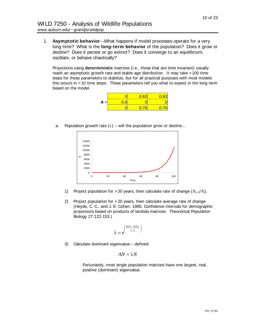
1. Asymptotic behavior—What happens if model processes operate for a very long time? What is the long-term behavior of the population? Does it grow or decline? Does it persist or go extinct? Does it converge to an equilibrium, oscillate, or behave chaotically?

Projections using deterministic matrices (i.e., those that are time invariant) usually reach an asymptotic growth rate and stable age distribution. It may take >100 time steps for these parameters to stabilize, but for all practical purposes with most models this occurs in <10 time steps. These parameters tell you what to expect in the long term based on the model.

0 0.63 0.63A = 0.6 0 0

0 0.76 0.76

a. Population growth rate (λ) – will the population grow or decline…

0

2000

4000

6000

8000

10000

12000

14000

0 20 40 60 80 1

Time

00

1) Project population for >20 years, then calculate rate of change (Nt+1/Nt).

2) Project population for >20 years, then calculate average rate of change (Heyde, C. C., and J. E. Cohen. 1985. Confidence intervals for demographic projections based on products of lambda matrices. Theoretical Population Biology 27:122-153.)

⎟⎟⎠

⎞⎜⎜⎝

⎛−−

=λ 1lnln 1

tNN t

e

NAN

3) Calculate dominant eigenvalue – defined:

= λ

Fortunately, most single population matrices have one largest, real, positive (dominant) eigenvalue.

lect_12.doc

11 of 23


0.55

0.65

0.75

0.85

0.95

1.05

1.15

1.25

1.35

1.45

0 20 40 60 80 100Time

λ10.11

lnln 1

==λ⎟⎟⎠

⎞⎜⎜⎝

⎛−−

tNN t

e

Dominant eigenvalue = 1.10

Nt+1/Nt = 1.10

b. Stable age (stage) distribution (SAD) – What is the predicted structure of the population?

1) Project the population for >20 years, determine the percentage of the population in each age (stage) class.

0

1000

2000

3000

4000

5000

6000

0 20 40 60 80 100

Time

N

n(1 t)n(2 t)n(3 t)

2) Calculate the right eigenvector of the dominant eigenvalue and normalize.

Age/stage structure R eigenvectorFinal SAD

36.4% 36.4%19.8% 19.8%43.9% 43.9%

lect_12.doc

12 of 23


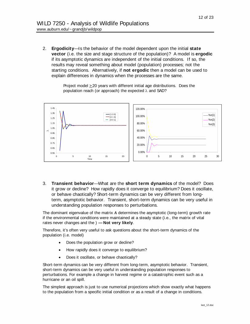
2. Ergodicity—Is the behavior of the model dependent upon the initial state vector (i.e. the size and stage structure of the population)? A model is ergodic if its asymptotic dynamics are independent of the initial conditions. If so, the results may reveal something about model (population) processes; not the starting conditions. Alternatively, if not ergodic then a model can be used to explain differences in dynamics when the processes are the same.

Project model >20 years with different initial age distributions. Does the population reach (or approach) the expected λ and SAD?

0.55

0.65

0.75

0.85

0.95

1.05

1.15

1.25

1.35

1.45

0 5 10 15 20Time

λ

[1 0 0][0 1 0][0 0 1]

0.00%

20.00%

40.00%

60.00%

80.00%

100.00%

120.00%

0 5 10 15 20 25 30

%n(1)%n(2)%n(3)

3. Transient behavior—What are the short term dynamics of the model? Does it grow or decline? How rapidly does it converge to equilibrium? Does it oscillate, or behave chaotically? Short-term dynamics can be very different from long-term, asymptotic behavior. Transient, short-term dynamics can be very useful in understanding population responses to perturbations.

The dominant eigenvalue of the matrix A determines the asymptotic (long-term) growth rate if the environmental conditions were maintained at a steady state (i.e., the matrix of vital rates never changes and the ) — Not very likely.

Therefore, it’s often very useful to ask questions about the short-term dynamics of the population (i.e. model)

• Does the population grow or decline?

• How rapidly does it converge to equilibrium?

• Does it oscillate, or behave chaotically?

Short-term dynamics can be very different from long-term, asymptotic behavior. Transient, short-term dynamics can be very useful in understanding population responses to perturbations. For example a change in harvest regime or a catastrophic event such as a hurricane or an oil spill.

The simplest approach is just to use numerical projections which show exactly what happens to the population from a specific initial condition or as a result of a change in conditions.

lect_12.doc

13 of 23


Example

Spectacled Eider population on the Y-K Delta at Kashunuk River Study site Demographics:

Age 1 Age 2 Age 3

Nest success 0.47 0.47

Clutch size (females hatched) 2.15 2.15

Breeding propensity 0.56 1

Duckling survival 0.34 0.34

Survival of immatures 0.49 0.49

Survival of adults

- exposed to lead 0.44 0.44

- not exposed 0.82 0.82 0.82

- lead exposure 0 0.1764 0.315

weighted average 0.75 0.70

( ) ( )( ) ( ) nll

nll

SleSlePSlebpSlebpP

****1**

3

2

+=−+=

nl

iiiii

SPSdsbpfhnsF ****

1

0

==

Matrix model:

0.000 0.094 0.1680.820 0 0A =

0 0.75 0.70

Life cycle graph:

1 2 3

lect_12.doc

14 of 23


Matrix analysis: Eigenvalues Eigenvectors (R&L) Real Imaginary Age/stage structReprod val0.858046 0 15.3% 0.9489 -0.07887 -0.22765 14.7% 0.992927-0.07887 0.227654 70.0% 1.012684

Numerical projection starting with SAD:

lect_12.doc

0

20

40

60

80

100

120

0 10 20 30 40 50

Year

N(t)

0.7600

0.78000.8000

0.8200

0.8400

0.86000.8800

0.9000

N(b t) SAD N(t+1)/N(t) SAD

Numerical projection after breeding failure:

0

20

40

60

80

100

120

0 10 20 30 40 50Year

N(t)

0.7600

0.7800

0.8000

0.8200

0.8400

0.8600

0.8800

0.9000

N(b t) N(b t) SAD N(t+1)/N(t) N(t+1)/N(t) SAD

15 of 23


Transient behavior after reproductive failure

020406080

100120

0 1 2 3 4 5

N(t)

0.7500

0.8000

0.8500

0.9000

÷

Year

N(b t) N(b t) SADN(t+1)/N(t) N(t+1)/N(t) SAD

Numerical projection after loss of 80% of adult females

020406080

100120

N(b t) N(b t) SAD

lect_12.doc

0 10 20 30 40 50

N(t)

0.0

0.5

1.0

1.5

♦

Year

N(t+1)/N(t) N(t+1)/N(t) SAD

Transient dynamics after loss of 80% of adult females

N(b t) N(b t) SAD

020406080

100120

0 1 2 3 4 5

Year

N(t

)

0.0

0.5

1.0

1.5

N(t+1)/N(t) N(t+1)/N(t) SAD

The rate of convergence on a stable population growth rate is governed by the relative size of the subdominant eigenvalues. That is, the larger λ1 is in relation to λi>1 the more rapidly the population will converge on stability. This property often referred to as the damping ratio is defined as:

16 of 23


2λ1λ

=ρ .

It follows then that for larger values of ρ the population converges more rapidly on λ1 and SAD.

Example:

Hypothetical population matrix with high Fi and low annual survival, similar to a small mammal or a passerine bird:

0 3 4

0.2 0 0 A =

0 0.4 0.4

Eigenvalues Eigenvectors (R&L)

Real Imaginary Age/stage structReprod val1.046434 0 76.4% 0.479315-0.15583 0 14.6% 2.507855-0.49061 0 9.0% 2.965901

N(b t)

lect_12.doc

0

50

100

150

200

250

300

350

0 5 10 15 20Year

N(t)

0

0.5

1

1.5

2

2.5

N(b t) SAD N(t+1)/N(t) N(t+1)/N(t) SAD

ρ = 6.7

17 of 23


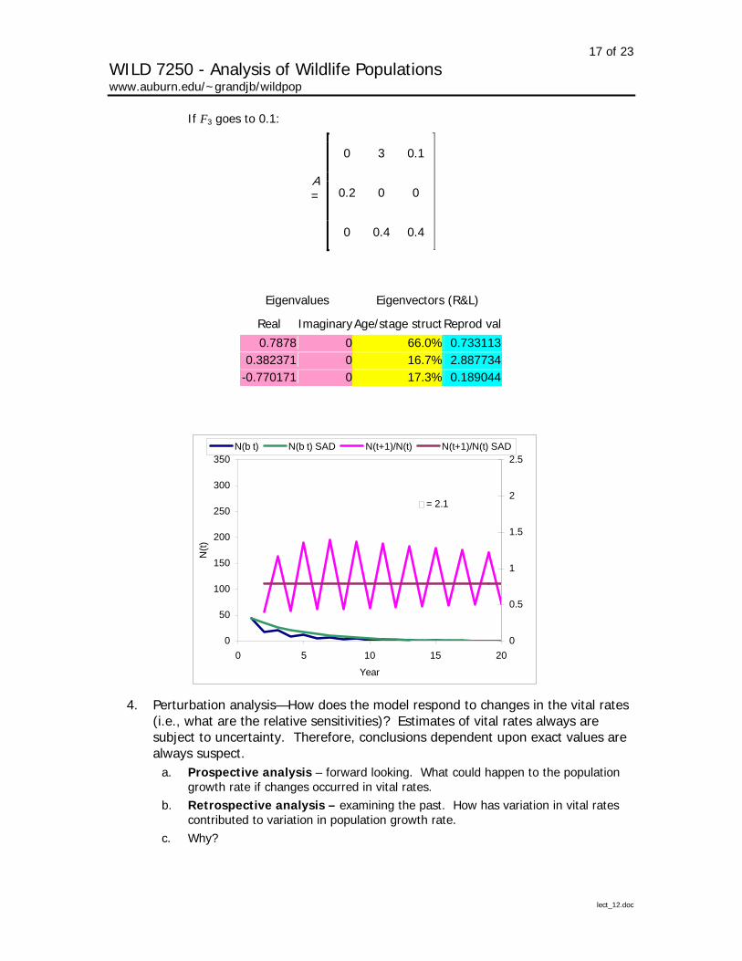
If F3 goes to 0.1:

0 3 0.1

0.2 0 0 A =

0 0.4 0.4


Real ImaginaryAge/stage structReprod val

0.7878 0 66.0% 0.7331130.382371 0 16.7% 2.887734

-0.770171 0 17.3% 0.189044

lect_12.doc

0

50

100

150

200

250

300

350

0 5 10 15 20

Year

N(t)

0

0.5

1

1.5

2

2.5N(b t) N(b t) SAD N(t+1)/N(t) N(t+1)/N(t) SAD

= 2.1

4. Perturbation analysis—How does the model respond to changes in the vital rates (i.e., what are the relative sensitivities)? Estimates of vital rates always are subject to uncertainty. Therefore, conclusions dependent upon exact values are always suspect.

a. Prospective analysis – forward looking. What could happen to the population growth rate if changes occurred in vital rates.

b. Retrospective analysis – examining the past. How has variation in vital rates contributed to variation in population growth rate.

c. Why?

18 of 23


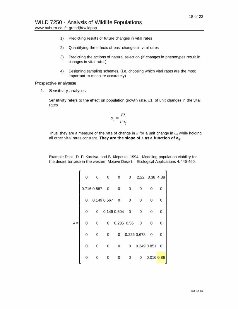
1) Predicting results of future changes in vital rates

2) Quantifying the effects of past changes in vital rates

3) Predicting the actions of natural selection (if changes in phenotypes result in changes in vital rates)

4) Designing sampling schemes. (i.e. choosing which vital rates are the most important to measure accurately)

Prospective analysese

1. Sensitivity analyses

Sensitivity refers to the effect on population growth rate, λ1, of unit changes in the vital rates.

lect_12.doc

ijij a

s∂

λ∂=

Thus, they are a measure of the rate of change in λ for a unit change in aij while holding all other vital rates constant. They are the slope of λ as a function of aij.

Example Doak, D. P. Kareiva, and B. Klepetka. 1994. Modeling population viability for the desert tortoise in the western Mojave Desert. Ecological Applications 4:446-460.

0 0 0 0 0 2.22 3.38 4.38

0.716 0.567 0 0 0 0 0 0

0 0.149 0.567 0 0 0 0 0

0 0 0.149 0.604 0 0 0 0

A = 0 0 0 0.235 0.56 0 0 0

0 0 0 0 0.225 0.678 0 0

0 0 0 0 0 0.249 0.851 0

0 0 0 0 0 0 0.016 0.86

19 of 23


lect_12.doc


Real Imaginary Age/stage structReprod val

0.981896 0 24.7% 0.196423

0.838824 0 42.7% 0.269367

0.780062 0.256278 15.3% 0.750061

0.780062 -0.25628 6.0% 2.08857

0.494042 0 3.4% 3.35856

0.412547 -0.2158 2.5% 6.297609

0.412547 0.215801 4.7% 5.93477

-0.01298 0 0.6% 7.057933

Sensitivity matrix

0 0 0 0 0 0.004895 0.009312 0.001222

0.066615 0.114961 0 0 0 0 0 0

0 0.320112 0.114961 0 0 0 0 0

0 0 0.320112 0.126216 0 0 0 0

0 0 0 0.202964 0.113053 0 0 0

0 0 0 0 0.211985 0.156951 0 0

0 0 0 0 0 0.147908 0.281362 0

0 0 0 0 0 0 0.33461 0.043921

20 of 23


0.98

0.981

0.982

0.983

0.984

0.985

0.986

0.987

0.988

0.989

0.82 0.84 0.86 0.88 0.90 0.92 0.94

a(8,8)

λ

P(l)

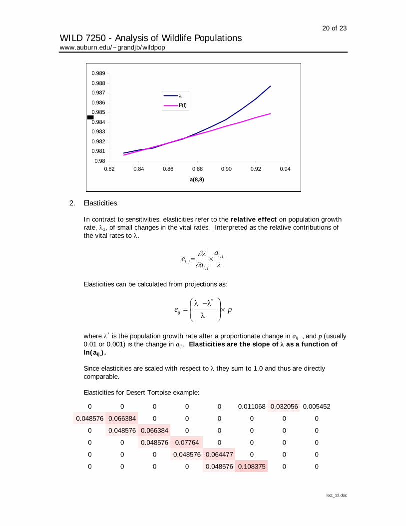
2. Elasticities

In contrast to sensitivities, elasticities refer to the relative effect on population growth rate, λ1, of small changes in the vital rates. Interpreted as the relative contributions of the vital rates to λ.

∂λ aλ∂

ji

jiji a

e ,

,, ×=

Elasticities can be calculated from projections as:

lect_12.doc

peij ×⎟⎟⎠

⎞⎜⎜⎝

⎛

λ

λ−λ=

*

where λ* is the population growth rate after a proportionate change in aij , and p (usually 0.01 or 0.001) is the change in aij.. Elasticities are the slope of λ as a function of ln(aij.).

Since elasticities are scaled with respect to λ they sum to 1.0 and thus are directly comparable.

Elasticities for Desert Tortoise example:

0 0 0 0 0 0.011068 0.032056 0.005452

0.048576 0.066384 0 0 0 0 0 0

0 0.048576 0.066384 0 0 0 0 0

0 0 0.048576 0.07764 0 0 0 0

0 0 0 0.048576 0.064477 0 0 0

0 0 0 0 0.048576 0.108375 0 0

21 of 23


lect_12.doc

0 0 0 0 0 0.037508 0.243854 0

0 0 0 0 0 0 0.005452 0.038468

Thus, it would be correct to state that P7 (e77 = 0.24) the probability of surviving and remaining in stage 7 has 2.25 times as much of an effect on λ as does P6 (e66 = 0.11)

Also, elasticities can be summed to determine the relative contributions of more than one vital rate. Thus, it would also be correct to conclude that the elasticity of transition probabilities (Ps and Gs) was 0.95, while the elasticity of Fs was .05; thus, the population is 20 times as sensitive to survival rates versus productivity rates.

Retrospective analysis – Life Table Response Experiments (LTRE)

A set of vital rates is the response variable in an experimental design. The treatments affect the various vital rates and the demographic models represent a way to synthesize the results. λ is the most frequently use statistic to evaluate the effect of the treatments. As such they are often used to examine the effect of past variation in vital rates on population growth rates.

LTRE designs are often analogous to analysis of variance and are presented as fixed (one-way, two-way, or factorial), random or regression analysis.

Example – one-way fixed design one treatment (t) and one control (c) the resulting vital rates are used to populate the matrices:

0 0 0 0 0 2.22 3.38 4.38

0.716 0.567 0 0 0 0 0 0

0 0.149 0.567 0 0 0 0 0

0 0 0.149 0.604 0 0 0 0

0 0 0 0.235 0.56 0 0 0

0 0 0 0 0.225 0.678 0 0

0 0 0 0 0 0.249 0.851 0

At =

0 0 0 0 0 0 0.016 0.86

0 0 0 0 0 0.042 0.069 0.069

0.716 0.567 0 0 0 0 0 0

0 0.149 0.567 0 0 0 0 0

0 0 0.149 0.604 0 0 0 0

0 0 0 0.235 0.56 0 0 0

0 0 0 0 0.225 0.678 0 0

0 0 0 0 0 0.249 0.851 0

Ac =

0 0 0 0 0 0 0.016 0.86

22 of 23


The mean or reference matrix is calculated as:

lect_12.doc

2/)( ctm AAA += ,

0 0 0 0 0 1.1311.72452.2245

0.716 0.567 0 0 0 0 0 0

0 0.1490.567 0 0 0 0 0

0 0 0.1490.604 0 0 0 0

0 0 0 0.235 0.56 0 0 0

0 0 0 0 0.2250.678 0 0

0 0 0 0 0 0.249 0.851 0

Am =

0 0 0 0 0 0 0.016 0.86

the sensitivities of Am are calculated:

0.000 0.000 0.000 0.000 0.000 0.006 0.016 0.003

0.056 0.104 0.000 0.000 0.000 0.000 0.000 0.000

0.000 0.268 0.104 0.000 0.000 0.000 0.000 0.000

0.000 0.000 0.268 0.115 0.000 0.000 0.000 0.000

0.000 0.000 0.000 0.170 0.102 0.000 0.000 0.000

0.000 0.000 0.000 0.000 0.178 0.146 0.000 0.000

0.000 0.000 0.000 0.000 0.000 0.132 0.324 0.000

mAS =

0.000 0.000 0.000 0.000 0.000 0.000 0.374 0.065

The difference (D) between At and Ac is then multiplied (elementwise) by the sensitivities:

0 0 0 0 0 2.178 3.311 4.311

0 0 0 0 0 0 0 0

0 0 0 0 0 0 0 0

0 0 0 0 0 0 0 0

0 0 0 0 0 0 0 0

0 0 0 0 0 0 0 0

0 0 0 0 0 0 0 0

D =

0 0 0 0 0 0 0 0

23 of 23


0 0 0 0 0 0.0138 0.0515 0.0116

0 0 0 0 0 0 0 0

0 0 0 0 0 0 0 0

0 0 0 0 0 0 0 0

0 0 0 0 0 0 0 0

0 0 0 0 0 0 0 0

0 0 0 0 0 0 0 0

mASD =

0 0 0 0 0 0 0 0

The resulting matrix is the contributions of the differences in the vital rates to the change in the population growth rate.

lect_12.doc

Documents

Lecture 12 –Matrix Models for Population Biologygrandjb/wildpop/lectures/lect_12.pdf · The age-structured transition matrix model representing this system ... Life cycle graph