Embed Size (px)
Citation preview
Lecture 12
Lecture 12: Feasible direction methods
Kin Cheong SouDecember 2, 2013
TMA947 – Lecture 12 Lecture 12: Feasible direction methods 1 / 1
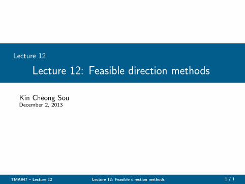
Feasible-direction methods, I Intro
◮ Consider the problem to find
f ∗ = infimum f (x), (1a)
subject to x ∈ X , (1b)
X ⊆ Rn nonempty, closed and convex; f : Rn → R is C 1 on X
◮ A natural idea is to mimic the line search methods forunconstrained problems.
◮ However, most methods for (1) manipulate (that is, relax) theconstraints defining X ; in some cases even such that thesequence {xk} is infeasible until convergence. Why?
TMA947 – Lecture 12 Lecture 12: Feasible direction methods 3 / 1
Feasible-direction methods, I Intro
◮ Consider a constraint “gi (x) ≤ bi ,” where gi is nonlinear
◮ Checking whether p is a feasible direction at x , or what themaximum feasible step from x in the direction of p is, is verydifficult
◮ For which step length α > 0 is gi (x + αp) = bi? This is anonlinear equation in α!
◮ Assuming that X is polyhedral, these problems are not present
◮ Note: KKT always necessary for a local min for polyhedralsets; methods will find such points
TMA947 – Lecture 12 Lecture 12: Feasible direction methods 4 / 1
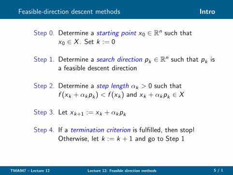
Feasible-direction descent methods Intro
Step 0. Determine a starting point x0 ∈ Rn such that
x0 ∈ X . Set k := 0
Step 1. Determine a search direction pk ∈ Rn such that pk is
a feasible descent direction
Step 2. Determine a step length αk > 0 such thatf (xk + αkpk) < f (xk) and xk + αkpk ∈ X
Step 3. Let xk+1 := xk + αkpk
Step 4. If a termination criterion is fulfilled, then stop!Otherwise, let k := k + 1 and go to Step 1
TMA947 – Lecture 12 Lecture 12: Feasible direction methods 5 / 1
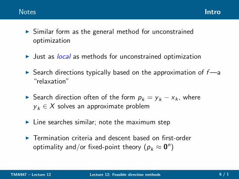
Notes Intro
◮ Similar form as the general method for unconstrainedoptimization
◮ Just as local as methods for unconstrained optimization
◮ Search directions typically based on the approximation of f—a“relaxation”
◮ Search direction often of the form pk = yk − xk , whereyk ∈ X solves an approximate problem
◮ Line searches similar; note the maximum step
◮ Termination criteria and descent based on first-orderoptimality and/or fixed-point theory (pk ≈ 0n)
TMA947 – Lecture 12 Lecture 12: Feasible direction methods 6 / 1
LP-based algorithm, I: The Frank–Wolfe method Frank–Wolfe
◮ The Frank–Wolfe method is based on a first-orderapproximation of f around the iterate xk . This means thatthe relaxed problems are LPs, which can then be solved byusing the Simplex method
◮ Remember the first-order optimality condition: If x∗ ∈ X is alocal minimum of f on X then
∇f (x∗)T(x − x∗) ≥ 0, x ∈ X ,
holds
◮ Remember also the following equivalent statement:
minimumx∈X
∇f (x∗)T(x − x∗) = 0
TMA947 – Lecture 12 Lecture 12: Feasible direction methods 9 / 1
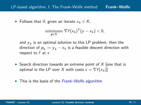
LP-based algorithm, I: The Frank–Wolfe method Frank–Wolfe
◮ Follows that if, given an iterate xk ∈ X ,
minimumy∈X
∇f (xk)T(y − xk) < 0,
and yk is an optimal solution to this LP problem, then thedirection of pk := yk − xk is a feasible descent direction withrespect to f at x
◮ Search direction towards an extreme point of X [one that isoptimal in the LP over X with costs c = ∇f (xk)]
◮ This is the basis of the Frank–Wolfe algorithm
TMA947 – Lecture 12 Lecture 12: Feasible direction methods 10 / 1
LP-based algorithm, I: The Frank–Wolfe method Frank–Wolfe
◮ We assume that X is bounded in order to ensure that the LPalways has a finite optimal solution. The algorithm can beextended to work for unbounded polyhedra
◮ The search directions then are either towards an extremepoint (finite optimal solution to LP) or in the direction of anextreme ray of X (unbounded solution to LP)
◮ Both cases identified in the Simplex method
TMA947 – Lecture 12 Lecture 12: Feasible direction methods 11 / 1
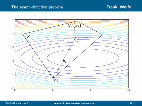
The search-direction problem Frank–Wolfe
−5 0 5 10−5
0
5
10
15
20
xk
yk
pk
∇f (xk)
X
TMA947 – Lecture 12 Lecture 12: Feasible direction methods 12 / 1
Algorithm description, Frank–Wolfe Frank–Wolfe
Step 0. Find x0 ∈ X (for example any extreme point in X ).Set k := 0
Step 1. Find an optimal solution yk to the problem to
minimizey∈X
zk(y ) := ∇f (xk)T(y − xk) (2)
Let pk := yk − xk be the search direction
Step 2. Approximately solve the problem to minimizef (xk + αpk) over α ∈ [0, 1]. Let αk be the steplength
Step 3. Let xk+1 := xk + αkpk
Step 4. If, for example, zk(yk) or αk is close to zero, thenterminate! Otherwise, let k := k+1 and go to Step 1
TMA947 – Lecture 12 Lecture 12: Feasible direction methods 13 / 1
∗Convergence Frank–Wolfe
◮ Suppose X ⊂ Rn nonempty polytope; f in C 1 on X
◮ In Step 2 of the Frank–Wolfe algorithm, we either use anexact line search or the Armijo step length rule
◮ Then: the sequence {xk} is bounded and every limit point (atleast one exists) is stationary;
◮ {f (xk)} is descending, and therefore has a limit;
◮ zk(yk) → 0 (∇f (xk)Tpk → 0)
◮ If f is convex on X , then every limit point is globally optimal
TMA947 – Lecture 12 Lecture 12: Feasible direction methods 14 / 1
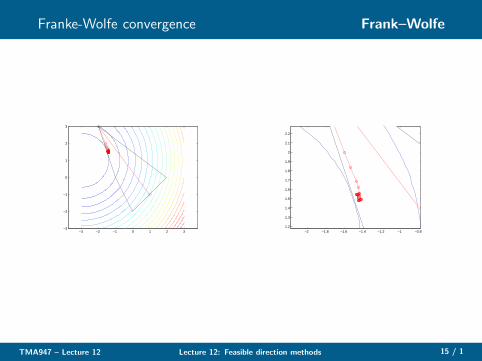
Franke-Wolfe convergence Frank–Wolfe
−3 −2 −1 0 1 2 3−3
−2
−1
0
1
2
3
−2 −1.8 −1.6 −1.4 −1.2 −1 −0.81.2
1.3
1.4
1.5
1.6
1.7
1.8
1.9
2
2.1
2.2
TMA947 – Lecture 12 Lecture 12: Feasible direction methods 15 / 1
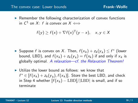
The convex case: Lower bounds Frank–Wolfe
◮ Remember the following characterization of convex functionsin C 1 on X : f is convex on X ⇐⇒
f (y ) ≥ f (x) +∇f (x)T(y − x), x , y ∈ X
◮ Suppose f is convex on X . Then, f (xk) + zk(yk) ≤ f ∗ (lowerbound, LBD), and f (xk) + zk(yk) = f (xk) if and only if xk isglobally optimal. A relaxation—cf. the Relaxation Theorem!
◮ Utilize the lower bound as follows: we know thatf ∗ ∈ [f (xk) + zk(yk), f (xk)]. Store the best LBD, and checkin Step 4 whether [f (xk)− LBD]/|LBD| is small, and if soterminate
TMA947 – Lecture 12 Lecture 12: Feasible direction methods 16 / 1
Notes Frank–Wolfe
◮ Frank–Wolfe uses linear approximations—works best foralmost linear problems
◮ For highly nonlinear problems, the approximation is bad—theoptimal solution may be far from an extreme point
◮ In order to find a near-optimum requires many iterations—thealgorithm is slow
◮ Another reason is that the information generated (the extremepoints) is forgotten. If we keep the linear subproblem, we cando much better by storing and utilizing this information
TMA947 – Lecture 12 Lecture 12: Feasible direction methods 17 / 1
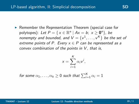
LP-based algorithm, II: Simplicial decomposition SD
◮ Remember the Representation Theorem (special case forpolytopes): Let P = { x ∈ R
n | Ax = b; x ≥ 0n}, benonempty and bounded, and V = {v1, . . . , vK} be the set ofextreme points of P. Every x ∈ P can be represented as aconvex combination of the points in V , that is,
x =K∑
i=1
αivi ,
for some α1, . . . , αk ≥ 0 such that∑
K
i=1 αi = 1
TMA947 – Lecture 12 Lecture 12: Feasible direction methods 19 / 1
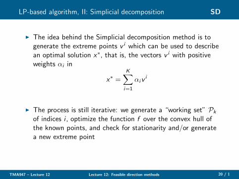
LP-based algorithm, II: Simplicial decomposition SD
◮ The idea behind the Simplicial decomposition method is togenerate the extreme points v i which can be used to describean optimal solution x∗, that is, the vectors v i with positiveweights αi in
x∗ =
K∑
i=1
αivi
◮ The process is still iterative: we generate a “working set” Pk
of indices i , optimize the function f over the convex hull ofthe known points, and check for stationarity and/or generatea new extreme point
TMA947 – Lecture 12 Lecture 12: Feasible direction methods 20 / 1
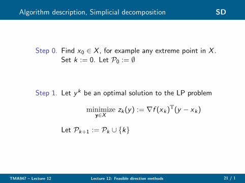
Algorithm description, Simplicial decomposition SD
Step 0. Find x0 ∈ X , for example any extreme point in X .Set k := 0. Let P0 := ∅
Step 1. Let yk be an optimal solution to the LP problem
minimizey∈X
zk(y) := ∇f (xk)T(y − xk)
Let Pk+1 := Pk ∪ {k}
TMA947 – Lecture 12 Lecture 12: Feasible direction methods 21 / 1
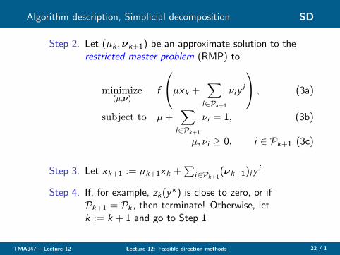
Algorithm description, Simplicial decomposition SD
Step 2. Let (µk ,νk+1) be an approximate solution to therestricted master problem (RMP) to
minimize(µ,ν)
f
µxk +∑
i∈Pk+1
νiyi
, (3a)
subject to µ+∑
i∈Pk+1
νi = 1, (3b)
µ, νi ≥ 0, i ∈ Pk+1 (3c)
Step 3. Let xk+1 := µk+1xk +∑
i∈Pk+1(νk+1)iy
i
Step 4. If, for example, zk(yk) is close to zero, or if
Pk+1 = Pk , then terminate! Otherwise, letk := k + 1 and go to Step 1
TMA947 – Lecture 12 Lecture 12: Feasible direction methods 22 / 1
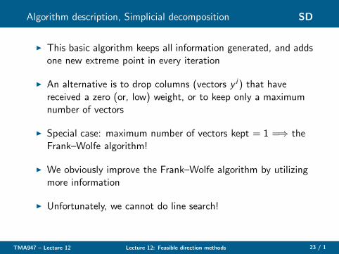
Algorithm description, Simplicial decomposition SD
◮ This basic algorithm keeps all information generated, and addsone new extreme point in every iteration
◮ An alternative is to drop columns (vectors y i ) that havereceived a zero (or, low) weight, or to keep only a maximumnumber of vectors
◮ Special case: maximum number of vectors kept = 1 =⇒ theFrank–Wolfe algorithm!
◮ We obviously improve the Frank–Wolfe algorithm by utilizingmore information
◮ Unfortunately, we cannot do line search!
TMA947 – Lecture 12 Lecture 12: Feasible direction methods 23 / 1
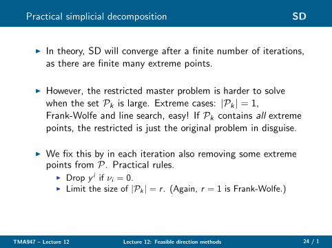
Practical simplicial decomposition SD
◮ In theory, SD will converge after a finite number of iterations,as there are finite many extreme points.
◮ However, the restricted master problem is harder to solvewhen the set Pk is large. Extreme cases: |Pk | = 1,Frank-Wolfe and line search, easy! If Pk contains all extremepoints, the restricted is just the original problem in disguise.
◮ We fix this by in each iteration also removing some extremepoints from P. Practical rules.
◮ Drop y i if νi = 0.◮ Limit the size of |Pk | = r . (Again, r = 1 is Frank-Wolfe.)
TMA947 – Lecture 12 Lecture 12: Feasible direction methods 24 / 1
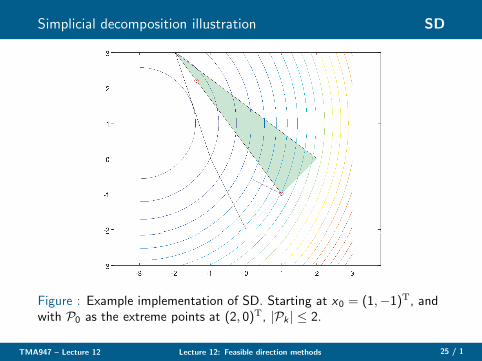
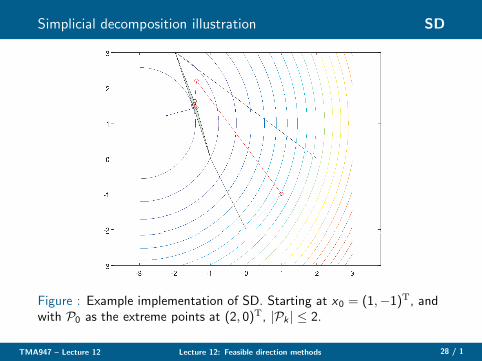
Simplicial decomposition illustration SD
Figure : Example implementation of SD. Starting at x0 = (1,−1)T, andwith P0 as the extreme points at (2, 0)T, |Pk | ≤ 2.
TMA947 – Lecture 12 Lecture 12: Feasible direction methods 25 / 1
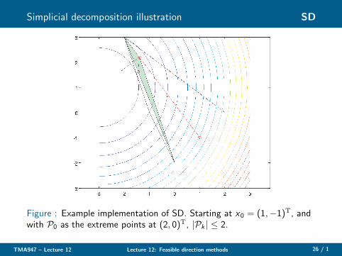
Simplicial decomposition illustration SD
Figure : Example implementation of SD. Starting at x0 = (1,−1)T, andwith P0 as the extreme points at (2, 0)T, |Pk | ≤ 2.
TMA947 – Lecture 12 Lecture 12: Feasible direction methods 26 / 1
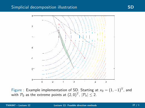
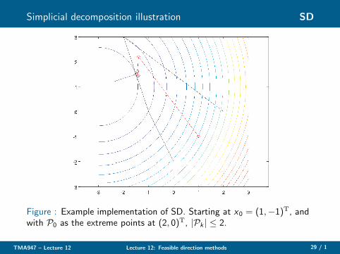
Simplicial decomposition illustration SD
Figure : Example implementation of SD. Starting at x0 = (1,−1)T, andwith P0 as the extreme points at (2, 0)T, |Pk | ≤ 2.
TMA947 – Lecture 12 Lecture 12: Feasible direction methods 27 / 1
Simplicial decomposition illustration SD
Figure : Example implementation of SD. Starting at x0 = (1,−1)T, andwith P0 as the extreme points at (2, 0)T, |Pk | ≤ 2.
TMA947 – Lecture 12 Lecture 12: Feasible direction methods 28 / 1
Simplicial decomposition illustration SD
Figure : Example implementation of SD. Starting at x0 = (1,−1)T, andwith P0 as the extreme points at (2, 0)T, |Pk | ≤ 2.
TMA947 – Lecture 12 Lecture 12: Feasible direction methods 29 / 1
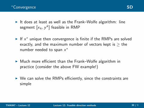
∗Convergence SD
◮ It does at least as well as the Frank–Wolfe algorithm: linesegment [xk , y
k ] feasible in RMP
◮ If x∗ unique then convergence is finite if the RMPs are solvedexactly, and the maximum number of vectors kept is ≥ thenumber needed to span x∗
◮ Much more efficient than the Frank–Wolfe algorithm inpractice (consider the above FW example!)
◮ We can solve the RMPs efficiently, since the constraints aresimple
TMA947 – Lecture 12 Lecture 12: Feasible direction methods 30 / 1
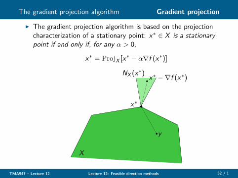
The gradient projection algorithm Gradient projection
◮ The gradient projection algorithm is based on the projectioncharacterization of a stationary point: x∗ ∈ X is a stationarypoint if and only if, for any α > 0,
x∗ = ProjX [x∗ − α∇f (x∗)]
���
���
X
y
x∗ −∇f (x∗)
x∗
NX (x∗)
TMA947 – Lecture 12 Lecture 12: Feasible direction methods 32 / 1
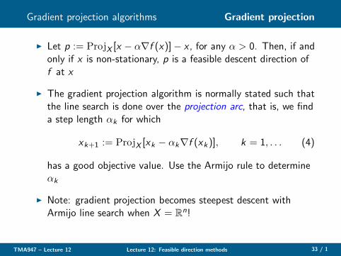
Gradient projection algorithms Gradient projection
◮ Let p := ProjX [x − α∇f (x)]− x , for any α > 0. Then, if andonly if x is non-stationary, p is a feasible descent direction off at x
◮ The gradient projection algorithm is normally stated such thatthe line search is done over the projection arc, that is, we finda step length αk for which
xk+1 := ProjX [xk − αk∇f (xk)], k = 1, . . . (4)
has a good objective value. Use the Armijo rule to determineαk
◮ Note: gradient projection becomes steepest descent withArmijo line search when X = R
n!
TMA947 – Lecture 12 Lecture 12: Feasible direction methods 33 / 1
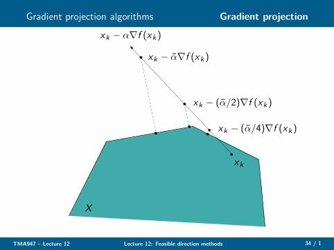
Gradient projection algorithms Gradient projection
X
xk
xk − α∇f (xk)
xk − (α/2)∇f (xk)
xk − (α/4)∇f (xk)
xk − α∇f (xk)
TMA947 – Lecture 12 Lecture 12: Feasible direction methods 34 / 1
Gradient projection algorithms Gradient projection
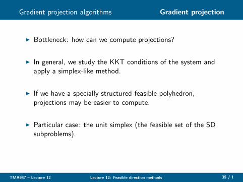
◮ Bottleneck: how can we compute projections?
◮ In general, we study the KKT conditions of the system andapply a simplex-like method.
◮ If we have a specially structured feasible polyhedron,projections may be easier to compute.
◮ Particular case: the unit simplex (the feasible set of the SDsubproblems).
TMA947 – Lecture 12 Lecture 12: Feasible direction methods 35 / 1
Easy projections Gradient projection
◮ Example: the feasible set isS = {x ∈ R
n | 0 ≤ xi ≤ 1, i = 1, . . . , n}.
◮ Then ProjS (x) = z, where
zi =
0, xi < 0,
xi , 0 ≤ xi ≤ 1
1, 1 < xi ,
for i = 1, . . . , n.
◮ Exercise: prove this by applying the varitional inequality (orKKT conditions) to the problem
minz∈S1
2‖x − z‖2
.
TMA947 – Lecture 12 Lecture 12: Feasible direction methods 36 / 1
∗Convergence, I Gradient projection
◮ X ⊆ Rn nonempty, closed, convex; f ∈ C 1 on X ;
◮ for the starting point x0 ∈ X it holds that the level setlevf (f (x0)) intersected with X is bounded
◮ In the algorithm (5), the step length αk is given by the Armijostep length rule along the projection arc
◮ Then: the sequence {xk} is bounded;
◮ every limit point of {xk} is stationary;
◮ {f (xk)} descending, lower bounded, hence convergent
◮ Convergence arguments similar to steepest descent one
TMA947 – Lecture 12 Lecture 12: Feasible direction methods 37 / 1
∗Convergence, II Gradient projection
◮ Assume: X ⊆ Rn nonempty, closed, convex;
◮ f ∈ C 1 on X ; f convex;
◮ an optimal solution x∗ exists
◮ In the algorithm (5), the step length αk is given by the Armijostep length rule along the projection arc
◮ Then: the sequence {xk} converges to an optimal solution
◮ Note: with X = Rn =⇒ convergence of steepest descent for
convex problems with optimal solutions!
TMA947 – Lecture 12 Lecture 12: Feasible direction methods 38 / 1
An illustration of FW vs. SD, I Gradient projection
◮ A large-scale nonlinear network flow problem which is used toestimate traffic flows in cities
◮ Model over the small city of Sioux Falls in North Dakota,USA; 24 nodes, 76 links, and 528 pairs of origin anddestination
◮ Three algorithms for the RMPs were tested—a Newtonmethod and two gradient projection methods. MATLABimplementation.
◮ Remarkable difference—The Frank–Wolfe method suffers fromvery small steps being taken. Why? Many extreme pointsactive = many routes used
TMA947 – Lecture 12 Lecture 12: Feasible direction methods 39 / 1
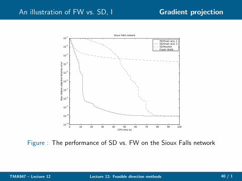
An illustration of FW vs. SD, I Gradient projection
0 10 20 30 40 50 60 70 80 90 10010
−11
10−10
10−9
10−8
10−7
10−6
10−5
10−4
10−3
10−2
10−1
Sioux Falls network
CPU time (s)
Max
rel
ativ
e ob
ject
ive
func
tion
erro
r
SD/Grad. proj. 1SD/Grad. proj. 2SD/NewtonFrank−Wolfe
Figure : The performance of SD vs. FW on the Sioux Falls network
TMA947 – Lecture 12 Lecture 12: Feasible direction methods 40 / 1