Embed Size (px)
Citation preview

F R E I G H T T R A V E L D E M A N D M O D E L I N G
C I V L 7 9 0 9 / 8 9 8 9
D E P A R T M E N T O F C I V I L E N G I N E E R I N G
U N I V E R S I T Y O F M E M P H I S
1
Lecture-10: Freight Mode Choice
11/14/2014

Outline2
1. Objective of Mode Choice
2. A simple Example
3. Discrete Choice Framework
4. The Random Utility Model
5. Binary Choice Models
6. Freight Mode Choice Models
7. Case Studies

Basics of Mode Choice (1)3
• Mode choice determines the number of trips between zones that are made by different modes (such as truck, rail, water, and air).
truck
rail

Basics of Mode Choice (2)4
1 2 3
1 a11 a12 a13
2 a21 a22 a23
3 a31 a32 a33
Trip Distribution
(Number of trips from origin->destination)
Mode Choice
(Number of trips from origin->destination
by mode)
1 2 3
1 𝑎11𝑚1 𝑎12
𝑚1 𝑎13𝑚1
2 𝑎21𝑚1 𝑎22
𝑚1 𝑎23𝑚1
3 𝑎31𝑚1 𝑎32
𝑚1 𝑎33𝑚1
1 2 3
1 𝑎11𝑚2 𝑎12
𝑚2 𝑎13𝑚2
2 𝑎21𝑚2 𝑎22
𝑚2 𝑎23𝑚2
3 𝑎31𝑚2 𝑎32
𝑚2 𝑎33𝑚21 2 3
1 𝑎11𝑚3 𝑎12
𝑚3 𝑎13𝑚3
2 𝑎21𝑚3 𝑎22
𝑚3 𝑎23𝑚3
3 𝑎31𝑚3 𝑎32
𝑚3 𝑎33𝑚3
𝑝𝑟𝑠𝑚1
𝑝𝑟𝑠𝑚2
𝑝𝑟𝑠𝑚3
𝑟
𝑠
𝑚𝑖
𝑝𝑟𝑠𝑚𝑖 = 1
Where,
r: origin
s: destination
mi: mode I
p: probability

Basics of Mode Choice (3)5
How to estimate the probability of choosing a mode
(𝑝𝑟𝑠𝑚𝑖)
Typically done by random utility maximization
Each mode is a choice given to the commodities to be carried from origin to destination
The attractiveness of each mode can be represented as an utility function
Derived from discrete choice theories
Let’s consider a simple example to get a glimpse of choice models

A Simple Example
6
Mobile Phone Choice
Education
Low(k=1) Medium(k=2) High(k=3)
Smartphone(i=1) 10 100 90 200
Feature phone (i=2) 140 200 60 400
150 300 150 600
25% 50% 25%
• Sample size: N = 600 (Random)
• Mobile phone choice (Smartphone, feature phone)
• Education (Low, Medium, high)

Example: Marginal and Joint Probabilities
• (Marginal) probability of choosing smartphone: P(i = 1)
𝑃 𝑖 = 1 =200
600=
1
3
• (Joint) probability of choosing smartphone and having medium level education: P(i = 1, k =2)
𝑃 𝑖 = 1, 𝑘 = 2 =100
600=
1
6
𝑖=1
2
𝑘=1
3
𝑝 𝑖, 𝑘 = 1

Joint and Marginal Probabilities
Mobile Phone ChoiceEducation Mobile Phone
Choice MarginalLow(k=1) Medium(k=2) High(k=3)
Smartphone(i=1)10
600=
1
60
10
600=
1
60
90
600=
3
20
200
600=
1
3
Feature phone (i=2)140
600=
7
30
200
600=
1
3
60
600=
1
10
400
600=
2
3
Educational Marginal
150
600=
1
4
300
600=
1
2
150
600=
1
4

Example: Conditional Probability P(i|k)
• Bayes’ Theorem: P(i,k) = P(i) . P(k | i)
= P(k) . P(i | k)
Independence
P(i,k)=P(i)P(k)
P(i | k)=P(i)
P(k | i)=P(k)
𝑃 𝑖 =
𝑘
𝑃 𝑖, 𝑘
𝑃 𝑘 =
𝑖
𝑃 𝑖, 𝑘
𝑃 𝑘|𝑖 =P(i,k)
P(i), 𝑃(𝑖) ≠ 0
𝑃 𝑖|𝑘 =P(i,k)
P(k), 𝑃(𝑘) ≠ 0

Example: Modeling P(i | k)
• Behavioral Model- Probability (Mobile Phone Choice | Education) = P(i | k)
- Explains choice of mobile phone type given education level
• Unknown parameters
P(i =1| k=1) = 𝜋1
P(i =1| k=2) = 𝜋2
P(i =1| k=3) = 𝜋3

Example: Model Estimation
• Estimates of the unknown parameters:
𝜋1 = 𝑃 𝑖 = 1 𝑘 = 1 = 𝑃(𝑖 = 1, 𝑘 = 1)
𝑃(𝐾 = 1)=
160
14
=1
15= 0.067
𝜋2 = 𝑃 𝑖 = 1 𝑘 = 2 = 𝑃(𝑖 = 1, 𝑘 = 2)
𝑃(𝐾 = 2)=
16
12
=1
3= 0.333
𝜋3 = 𝑃 𝑖 = 1 𝑘 = 3 = 𝑃(𝑖 = 1, 𝑘 = 3)
𝑃(𝐾 = 3)=
320
14
=3
5= 0.6

Maximum Likelihood Estimation12
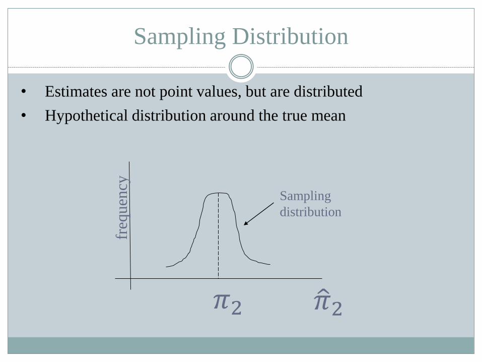
Sampling Distribution
• Estimates are not point values, but are distributed
• Hypothetical distribution around the true meanfr
equen
cy
Sampling
distribution
𝜋2 𝜋2

Standard Errors
• Compute the standard error of the estimates
• Since outcomes are Bernoulli random variables
𝑠1 = 𝜋1. (1 − 𝜋1)
𝑁1=
1/15. (1 − 1/15)
150= 0.020
𝑠2 = 𝜋2. (1 − 𝜋2)
𝑁2=
1/3. (1 − 1/3)
300= 0.027
𝑠3 = 𝜋3. (1 − 𝜋3)
𝑁3=
3/5. (1 − 3/5)
150= 0.040
Standard errors

Standard Error of Forecast
• Predicted smartphone share:
𝑃 𝑖 = 1 =
𝑘=1
3
𝜋𝑘 . 𝑃 𝑘
• The estimated standard of the predicted smartphone share is
𝑆 𝑝(𝑖=1) =
𝑘=1
3
𝑃 𝑘 2𝑠𝑘2 ≈ 0.0175 = 1.75%

Discrete Choice Framework
• Decision-Maker
- Individual (person/household)
- Socio-economic characteristics (e.g. age, gender, education, income)
• Alternatives
- Decision-maker n selects one and only one alternative from a choice set
Cn = {1,2,…,i,…,Jn} with Jn alternatives
• Attributes of alternatives (e.g. price, quality)
• Decision Rule
- Dominance, satisfaction, utility etc.

Mobile Phone Choice
• Decision Maker: An individual or a household
• Choice set: Alternative mobile phones
• Decision rule: Utility maximization
• Utility function: Function of attributes of the mobile phone, such as price and quality

Decision Maker Choice
Utility maximization
- Decision maker chooses the alternative that has the maximum utility (and falls within the set of considered alternatives)
If U(smartphone)>U(feature phone), choose smartphone
If U(smartphone)<U(feature phone), choose feature phone
U(smartphone) = ?
U(feature phone) = ?

Constructing the Utility Function
• U(smartphone)= U(pricesmartphone, qualitysmartphone, …)
U(feature phone)= U(pricefeaturephone, qualityfeaturephone, …)
• Assume linearity (in the parameters)
U(smartphone) = 𝛽1 × (pricesmartphone) + 𝛽2 ×(qualitysmartphone) + …
• Parameters represent tastes, which may bary across people
- Include socio-economic characteristics )e.g. age, gender, income)
- U(smartphone) = 𝛽1 × (pricesmartphone/income) + …
+ 𝛽2 × (qualitysmartphone)

Decision Maker Choice
If U(smartphone) - U(feature phone) > 0 , Probability(smartphone) = 1
If U(smartphone) - U(feature phone) < 0 , Probability(smartphone) = 0
1
00
P(smartphone)
U(smartphone) - U(feature phone)

Probabilistic Choice
• Random Utility Model (RUM)
Ui = V(attributes of I; parameters) + ɛi
• What is in the ɛ ? Analysts’ imperfect knowledge
- Unobserved attributes
- Unobserved taste variations
- Measurement errors
- Use of proxy variables
• U(smartphone) = 𝛽1 × (pricesmartphone) + 𝛽2 ×(qualitysmartphone) + … +
ɛsmartphone= V(smartphone) + ɛsmartphone

Probabilistic Binary Choice
1
00
P(smartphone)
V(smartphone) - V(feature phone)

3. The Random Utility Model
• Decision rule: Utility maximization
- Individual n selects the alternative i with the highest utility Uin
among those in the choice set Cn
• Utility: Uin = Vin + ɛin
• Vin: Systematic utility expressed as a function of k observable variables,
e.g. 𝑘 𝛽𝑘𝑥𝑖𝑛𝑘 = 𝛽′𝑥𝑖𝑛
• ɛin : Random utility component

The Random Utility Model (Cont.)
• Choice Probability
P(i|Cn) = P(Uin ≥ Ujn ∀ j ∈ Cn)
= P(Uin - Ujn ≥ 0,∀ j ∈ Cn)
= P(Uin = maxj Ujn ,∀ j ∈ Cn)
• For binary choice,
Pn(1) = P(U1n ≥ U2n)
= P(U1n − U2n ≥ 0)

Example with Attributes
𝑈1 = 𝛽1𝑞1 − 𝛽2𝑝1 + 𝜀1𝑈2 = 𝛽1𝑞2 − 𝛽2𝑝2 + 𝜀2
𝛽1, 𝛽2 ≥ 0
Mobile Phone ChoiceAttributes
UtilityQuality (q) Price (p)
Smartphone(i=1) 𝑞1 𝑝1 𝑈1
Feature phone (i=2) 𝑞1 𝑝2 𝑈2

Example with Attributes(Cont.)
Ordinal utility
- Decision are based on utility differences
- Unique up to order preserving transformation
𝑈1 = (𝛽1𝑞1 − 𝛽2𝑝1 + 𝜀1 + 𝛼)𝜇∗
𝑈2 = (𝛽1𝑞2 − 𝛽2𝑝2 + 𝜀2 + 𝛼)𝜇∗
𝛽1, 𝛽2, 𝜇∗ ≥ 0

Example with Attributes(Cont.)
𝑈1 =𝛽1
𝛽2𝑞1 − 𝑝1 + 𝜀1
𝑈2 =𝛽1
𝛽2𝑞2 − 𝑝2 + 𝜀2
𝛽 =𝛽1
𝛽2= "𝑣𝑎𝑙𝑢𝑒 𝑜𝑓 𝑞𝑢𝑎𝑙𝑖𝑡𝑦"
𝑉1 =𝛽1
𝛽2𝑞1 − 𝑝1
𝑉2 =𝛽1
𝛽2𝑞2 − 𝑝2
𝑈1 − 𝑈2 = −𝛽1
𝛽2𝑞2 − 𝑞1 − 𝑝1 − 𝑝2 + 𝜀1 − 𝜀2
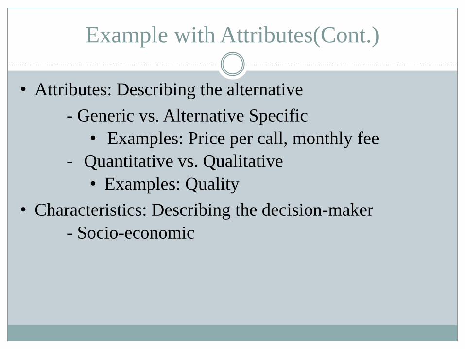
Example with Attributes(Cont.)
• Attributes: Describing the alternative
- Generic vs. Alternative Specific
• Examples: Price per call, monthly fee
- Quantitative vs. Qualitative
• Examples: Quality
• Characteristics: Describing the decision-maker
- Socio-economic

Random Terms
• Distribution of epsilons (ε)
• Variance/covariance structure
- Correlations between alternatives
- Multidimensional decision (e.g. mobile phone type and service provider)
• Typical models
- Probit (normal error terms)
- Logit (i.i.d. “Extreme Value” error terms)

4.Binary Choice Models
Choice Set Cn={1,2} ∀ n
Pn(1) = P(1| Cn)=P( U1n ≥ U2n)
= P(V1n + 𝜀1n ≥ V2n + 𝜀2n)
= P(V1n –V2n ≥ 𝜀2n - 𝜀1n)
= P(V1n –V2n ≥ 𝜀n)
= P(Vn ≥ 𝜀n)= F𝜀(Vn)

Binary Probit Model
“Probit” name comes from Probability Unit
𝜀1𝑛 ~ 𝑁(0, 𝜎12)
𝜀2𝑛 ~ 𝑁(0, 𝜎22)
𝜀𝑛 ~ 𝑁(0, 𝜎2) where 𝜎2 =𝜎12+𝜎2
2 − 2𝜎12
𝑓 𝜀 =1
𝜎 2𝜋𝑒−
12(
𝜀𝜎)2
𝑃𝑛 1 = 𝐹𝜀 𝑉𝑛 = −∞
𝑉𝑛 1
𝜎 2𝜋𝑒−
12(𝜀𝜎
)2
𝑑𝜀 = Φ(𝑉𝑛
𝜎)
Where Φ(z) is the standardized cumulative normal distribution

Binary Logit Model
“Logit” name comes from Logistic Probability Unit
𝜀1𝑛 ~ Extreme value(0, 𝜇) 𝐹𝜀 𝜀1𝑛 =exp[-𝑒−𝜇𝜀1𝑛]
𝜀2𝑛 ~ Extreme value(0, 𝜇) 𝐹𝜀 𝜀2𝑛 =exp[-𝑒−𝜇𝜀2𝑛]
𝜀𝑛 ~ Logistic (0, 𝜇) 𝐹𝜀 𝜀𝑛 =1
1+𝑒−𝜇𝜀𝑛
𝑃𝑛 1 = 𝐹𝜀 𝑉𝑛 =1
1 + 𝑒−𝜇𝜀𝑛

Logit vs Probit
• Probit
𝑃𝑛 1 = Φ𝑉𝑛
𝜎=
−∞
𝑉𝑛𝜎 1
2𝜋𝑒−
1
2𝜀2
𝑑𝜀 = −∞
𝑉1𝑛−𝑉2𝑛𝜎 1
2𝜋𝑒−
1
2𝜀2
𝑑𝜀
• Logit
𝑃𝑛 1 =1
1+𝑒−𝜇𝑉𝑛=
1
1+𝑒−𝜇(𝑉1𝑛−𝑉2𝑛) = 𝑒𝜇𝑉1𝑛
𝑒𝜇𝑉1𝑛+𝑒𝜇𝑉2𝑛
• 𝑉1𝑛 = 𝛽′𝑥1𝑛, 𝑉2𝑛 = 𝛽′𝑥2𝑛, 𝑉𝑛 = 𝛽′(𝑥1𝑛 − 𝑥2𝑛)

Why Logit?
• Probit does not have a closed form-the choice probability is an integral
• The logistic distribution is used because
• It approximates a normal distribution quite well
• It is analytically convenient
• Extreme Value distribution can be “justified” because of utility maximization
• Logit does have “fatter” tails than a normal distribution

Summary
• A simple Example
• Discrete Choice Framework
• The Random Utility Model
• Binary Choice Models
• Probit 𝑃𝑛 1 = Φ 𝑉𝑛 = −∞
𝑉𝑛 1
2𝜋𝑒−
1
2𝜀2
𝑑𝜀
(normalize σ = 1)
• Logit 𝑃𝑛 1 =1
1+𝑒−𝑉𝑛=
𝑒𝑉1𝑛
𝑒𝑉1𝑛+𝑒𝑉2𝑛
(normalize μ = 1)
• 𝑉1𝑛 = 𝛽′𝑥1𝑛, 𝑉2𝑛 = 𝛽′𝑥2𝑛, 𝑉𝑛 = 𝛽′(𝑥1𝑛 − 𝑥2𝑛)

Additional Readings
• Ben-Akiva, M. and Lerman, S. (1985), Discrete Choice Analysis: Theory and Application to Travel Demand, MIT Press, Cambridge MA, USA, Chapters 1-7.

Maximum Likelihood Estimation
Log likelihood function:𝐿 𝛽 = 𝑙𝑛𝐿∗ 𝛽 = 𝑛=1
𝑁 𝑙𝑛𝑃 𝑦𝑛 𝑋𝑛, 𝛽 = 𝑛=1𝑁 𝑖∈𝐶𝑛
𝑙𝑛𝑃 𝑖 𝐶𝑛
Where 𝑦𝑖𝑛 = 1if n chose alternative I, 0 otherwise
Logit:
𝑃 𝑖 𝐶𝑛 =𝑒𝜇𝑉𝑖𝑛
𝑗∈𝐶𝑛𝑒
𝜇𝑉𝑗𝑛, 𝜇 = 1
𝐿 𝛽 =
𝑛=1
𝑁
𝑖∈𝐶𝑛
𝑦𝑖𝑛 𝑉𝑖𝑛 − 𝑙𝑛
𝑗∈𝐶𝑛
𝑒𝑉𝑗𝑛

Maximum Likelihood Estimation(cont.)
The maximum likelihood estimation problem:
𝛽 = arg 𝑚𝑎𝑥𝛽𝐿(𝛽1, 𝛽2, … , 𝛽𝑘)
FOC for linear in parameters Logit
𝐿 𝛽 =
𝑛=1
𝑁
𝑖∈𝐶𝑛
𝑦𝑖𝑛 𝑉𝑖𝑛 − 𝑙𝑛
𝑗∈𝐶𝑛
𝑒𝑉𝑗𝑛 𝑉𝑖𝑛 = 𝑘=1
𝐾
𝛽𝑘𝑋𝑖𝑛𝑘
𝜕𝐿(𝛽)
𝜕𝛽𝑘=
𝑛=1
𝑁
𝑖∈𝐶𝑛
𝑦𝑖𝑛 𝑥𝑖𝑛𝑘 − 𝑗∈𝐶𝑛
𝑥𝑖𝑛𝑘𝑒𝑉𝑗𝑛
𝑗∈𝐶𝑛𝑒𝑉𝑗𝑛
= 0
𝑛=1
𝑁
𝑖∈𝐶𝑛
𝑦𝑖𝑛 − 𝑃𝑛 𝑖|𝑥𝑛, 𝛽 𝑥𝑖𝑛𝑘 = 0

Evaluation of Estimation Results
Signs and relative magnitudes of the coefficients For example, we expect the coefficient of price to be negative
Statistical tests
Goodness of fit measures

Statistical tests
Asymptotic t-test
- Used to test if a particular parameter is different from zero or from another known value
- Standard output statistic with most software
𝐻0: 𝛽𝑘 = 𝛽𝑘0
𝑡𝑘 = 𝛽𝑘 − 𝛽𝑘
0
𝑠 𝛽𝑘
- Compare to the critical value of the t distribution at a given level of significance

Statistical tests (cont.)
Likelihood ratio test- Tests nested hypotheses (restrictions in the model)
The statistic −2 𝐿 0 − 𝐿 𝛽
- Used to test the null hypothesis that all parameters are zero
- It is asymptotically 𝜒2 distributed with K (number of parameters) degrees of freedom
The statistic −2 𝐿 𝑐 − 𝐿 𝛽
- Used to test the null hypothesis that all the parameters other than
the intercept are zero
- It is asymptotically 𝜒2 distributed with K-1 (number of restrictions) degrees of freedom

Goodness of Fit
𝜌2 and 𝜌2 are analogous to 𝑅2 and 𝑅2 in least squares.
Likelihood ratio index 𝜌2: measures the fraction of an initial log likelihood that is explained by the model
𝜌2 ≡ 1 −𝐿( 𝛽)
𝐿(0)
𝜌2 is monotonic in the number of parameters K
𝜌2 must lie between 0 and 1.

Goodness of Fit
Adjusted 𝜌2 ( 𝜌2)
- Useful for comparison of models with different number of parameters (i.e., different degrees of freedom)
𝜌2 ≡ 1 −𝐿 𝛽 − 𝐾
𝐿(0)

Extensions of Binary Choice Models44
Classical extensions
Multinomial Logit (MNL)
NL (Nested Logit)
CNL (Cross Nested Logit)
MMNL (Mixed Multinomial Logit)
Logit fixed effect / random effect
Advanced
Latent class
Bayesian
Hybrid

Maryland Freight Mode Choice Model45
Source: Mishra, S., Zhu, X, and Fucca, F. “An integrated framework for Modeling freight mode and route choice” Report for Maryland State Highway Administration. [Download]

Growing awareness of freight system
Thrust at federal, state and local level
Maryland’s freight transportation is estimated
To grow about 105% by 2035
1.4 billion of total tons
4.98 trillion of $ value transfer (108% increase from 2006)
Sustainability of MD corridors to meet the future demand
Background

National Peak Period Congestion-2007 (Freight)

National Peak Period Congestion-2040 (Freight)

Why Freight Mode Choice?
Freight demand by mode varies by
Type of commodity
Value and size of commodity
Travel characteristics near distribution centers
Finer level geometric detail
Detailed Origin-Destination analysis within Maryland
Land use impact on freight flows
LOS identification and project selection
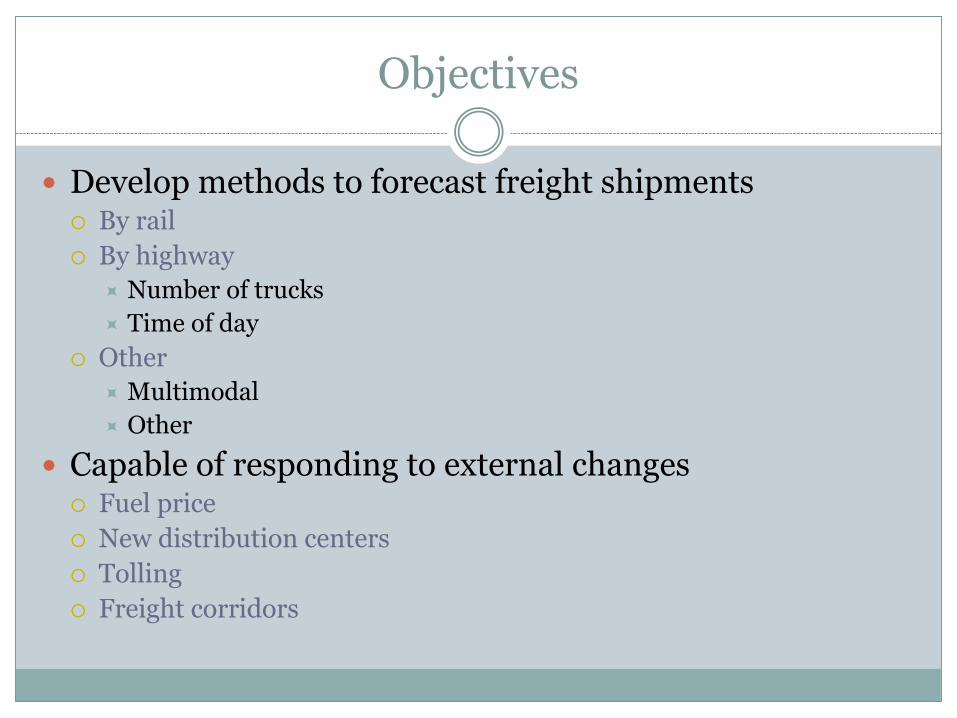
Objectives
Develop methods to forecast freight shipments By rail
By highway
Number of trucks
Time of day
Other
Multimodal
Other
Capable of responding to external changes Fuel price
New distribution centers
Tolling
Freight corridors

Mode Choice Factors
Develop methods to forecast freight shipments By rail
By highway
Number of trucks
Time of day
Other
Multimodal
Other
Capable of responding to external changes Fuel price
New distribution centers
Tolling
Freight corridors

Data
Available from Freight Analysis Framework (FAF)
Annual Macroscopic North American Freight Flow
Tons, Value, Distance, Commodity, Mode
Derive large scale long distance movements
Not available from FAF
Through trips (route)
Short distance internal trips
Cost (fuel price, time)
Just in time delivery
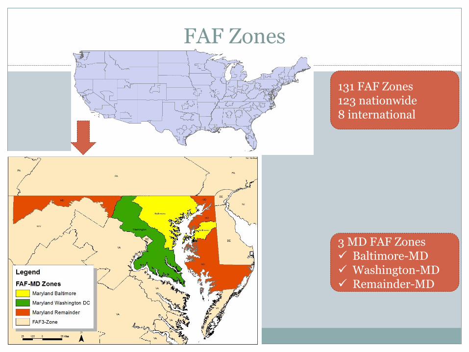
FAF Zones
131 FAF Zones123 nationwide8 international
3 MD FAF Zones Baltimore-MD Washington-MD Remainder-MD

Freight in Maryland
Within
MD
Leaving
MD
Arriving
in MD
Through
(Northeast-
Southeast)
Weight
(million of tons)135 84 91 52
Value (billion$) 92 113 169 177
Value/Weight
(Thousand $/ton)0.7 1.3 1.9 3.4
Northeast: CT, ME, MA, NH, NJ, NY, RI,VTSoutheast: FL, GA, NC, SC

External and Internal Trips By Mode
0.00%
10.00%
20.00%
30.00%
40.00%
50.00%
60.00%
70.00%
80.00%
90.00%
100.00%
Weight Value Weight Value Weight Value Weight Value
Within Maryland Leaving MD Arriving in MD Through (NE-SE)
Truck Rail Multimode Other
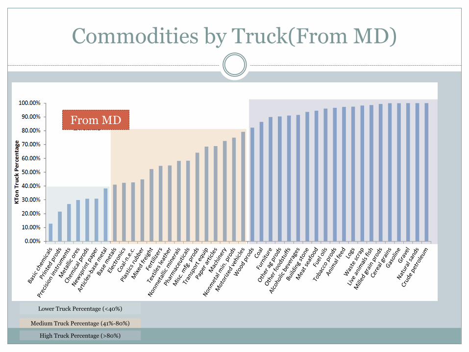
Commodities by Truck(From MD)
Lower Truck Percentage (<40%)
Medium Truck Percentage (41%-80%)
High Truck Percentage (>80%)
From MD

Commodities by Truck (To MD)
To MD
Lower Truck Percentage (<40%)
Medium Truck Percentage (41%-80%)
High Truck Percentage (>80%)

Commodities by Truck (Within MD)
Within MD
Lower Truck Percentage (<40%)
Medium Truck Percentage (41%-80%)
High Truck Percentage (>80%)

Proposed Model Structure
Within MD
Leaving MD
Arriving in MD
Com 1
Com 2
Com 3
4 models for different OD and Commodities
From To From To From To
1 Live animals fish 3 3 15 Coal 3 3 29 Printed prods 1 1
2 Cereal grains 3 3 16 Crude petroleum 3 3 30 Textiles leather 2 2
3 Other ag prods 3 3 17 Gasoline 3 3 31 Nonmetal min. prods 2 3
4 Animal feed 3 3 18 Fuel oils 3 3 32 Base metals 2 2
5 Meat seafood 3 3 19 Coal-n.e.c. 2 2 33 Articles-base metal 1 2
6 Milled grain prods 3 3 20 Basic chemicals 1 2 34 Machinery 2 2
7 Other foodstuffs 3 3 21 Pharmaceuticals 2 1 35 Electronics 2 2
8 Alcoholic beverages 3 3 22 Fertilizers 2 3 36 Motorized vehicles 2 1
9 Tobacco prods 3 3 23 Chemical prods 1 1 37 Transport equip 2 3
10 Building stone 3 3 24 Plastics rubber 2 1 38 Precision instruments 1 2
11 Natural sands 3 3 25 Logs 3 2 39 Furniture 3 2
12 Gravel 3 3 26 Wood prods 3 2 40 Misc. mfg. prods 2 2
13 Nonmetallic minerals 2 2 27 Newsprint paper 1 3 41 Waste scrap 3 3
14 Metallic ores 1 3 28 Paper articles 2 2 43 Mixed freight 2 2

Proposed Method
Aggregated analysis
Using land use as the factor
Logistic Regression Models
𝑃𝑖𝑗 is the probability of Truck Tonnage share
𝑋𝑖𝑗 is the Info of distribution centers,
highway/railway coverage,transportation/warehousing employment.
𝑙𝑜𝑔𝑖𝑡 𝑃𝑖𝑗 = 𝑋𝑖𝑗𝛽𝑗 + 𝜀𝑖𝑗

𝑙𝑜𝑔
𝑇𝑜.𝑑𝑤𝑜.𝑑
1 −𝑇𝑜.𝑑𝑤𝑜.𝑑
= 𝑋𝑖𝑗𝛽𝑗 + 𝜀𝑖𝑗
=𝛽0 + 𝛽1𝐷𝑖𝑠𝑡 + 𝛽2 𝐷𝐶𝑂 + 𝛽3 𝐷𝐶𝐷 + 𝛽4 𝐶𝑜𝑣𝑂 + 𝛽5 𝐶𝑜𝑣𝐷 +𝛽6 𝐸𝑚𝑝𝑂 + 𝛽7 𝐸𝑚𝑝𝐷 … + 𝜀𝑖𝑗
1 2 … 123
…
…
48 𝑤48.1 𝑤48.2 𝑤48.123
49 𝑤49.1
50 𝑤50.1 𝑤50.123
…
Summation of all group 1 tonnage from MD
1 2 … 123
…
…
48 𝑇48.1 𝑇48.2 𝑇48.123
49 𝑇49.1
50 𝑇50.1 𝑇50.123
…
Summation of all group 1 trucktonnage from MD
Proposed Model Structure

The share of truck 𝑃𝑡 =exp(𝑦)
1+exp(𝑦)
y = 0.431 − 0.002𝑋1 + 2.463𝑋2 − 0.164𝑋3 + 0.414𝑋4 − 0.024𝑋5 + 0.286𝑋6 −0.133𝑋7
Parameter Estimates95% CI Lower
95% CI Upper
Wald Chi-Square
Sig.
(Intercept) X0 .431 -2.580 3.442 .079 .779
Highway distance X1 -.002 -.003 -.001 19.315 .000
# Origin zone truck center
X2 2.463 .417 4.508 5.569 .018
# Origin zone rail center
X3 -.164 -.272 -.055 8.766 .003
# Destination zone truck center
X4 .414 .108 .720 7.018 .008
# Destination zone rail center
X5 -.024 -.056 .007 2.265 .132
# Destination zone port center
X6 .286 -.075 .647 2.412 .120
# Destination zone Trans employment
(10K)X7 -.133 -.310 .044 2.160 .142
Example: From MD group1

Example: From MD group1
Parameter Estimate
s
(Intercept) X0 .431
Highway distance X1 -.002
# Origin zone truck center
X2 2.463
# Origin zone rail center X3 -.164
# Destination zone truck center
X4 .414
# Destination zone rail center
X5 -.024
# Destination zone port center
X6 .286
# Destination zone Trans employment (10K)
X7 -.133
• For this group of commodities, the total truck share from MD is less than 40%.
• The truck percentage share decrease with longer distance between the Origin and Destination zone.
• The number of truck-truck centers in MD influence the truck share dramatically.
• More number of rail centers in MD reduce the truck share.
• Truck share is high to the destination zone with more truck and port oriented centers and less rail centers, and less transportation/warehousing employment.

Example: From MD group1
The total group 1 commodity shipped from Baltimore (MD MSA) to Denver (CO CSA) 𝑃𝑡=62.3%
If there is one more port related distribution center in Baltimore
The truck share does not change.
If there is one more truck center in Baltimore 𝑃𝑡=95.1%
If there is one more rail center in Baltimore 𝑃𝑡=58.3%

Example: From MD group1
If the Destination zone is Jacksonville (FL MSA) Distance reduces from 1,591 m to 756m.
Employment reduces from 5.17 to 3.22 10K.
𝑃𝑡=91.9%
With one more port-truck distribution center in Baltimore The truck share does not change.
If there is one more truck center in Baltimore 𝑃𝑡=99.3%
If there is one more rail center in Baltimore 𝑃𝑡=90.6%

Example: From MD group2
Parameter Estimates95% CI Lower
95% CI Upper
Wald Chi-
SquareSig.
(Intercept) X0 .689 -.542 1.920 1.204 .273
Highway distance X1 -.002 -.003 -.002 65.168 .000
# Destination zone rail center X2 -.022 -.044 .000 3.676 .055
Destination zone Principal arterialpercentage out of total highway and rail
mileageX3 3.660 .822 6.498 6.388 .011
# Destination zone Trans employment (10K) X4 .112 .013 .210 4.956 .026
For this group of commodities, the truck share from MD ranges from 40% to 80%.
The characteristics in Maryland do not impact the truck share.
The truck share only depends on the destination zone.
The truck is preferred to the zones closer to Maryland, with less rail distribution centers, higher Principal Arterial roadway and more transportation related employments.

Example: To MD group1
Parameter Estimat
es95% CI Lower
95% CI Upper
Wald Chi-Square
Sig.
(Intercept) X0 2.720 2.019 3.421 57.850 0.000
Highway distance X1 -0.001 -0.001 0.000 3.981 0.046
# Origin zone port related distribution center
X2 -0.158 -0.373 0.058 2.060 0.151
Destination zone rail center percentage X3 -2.020 -3.246 -0.794 10.431 0.001
# Origin zone Trans employment (10K) X4 0.040 -0.023 0.102 1.565 0.211
• The percentage of rail oriented distribution centers in Maryland is negative related with the truck share.
• The truck share also depends on the origin zone # port related centers, transportation employments.
• The truck is preferred from the zones closer to Maryland, with less port distribution centers, and more transportation related employments.
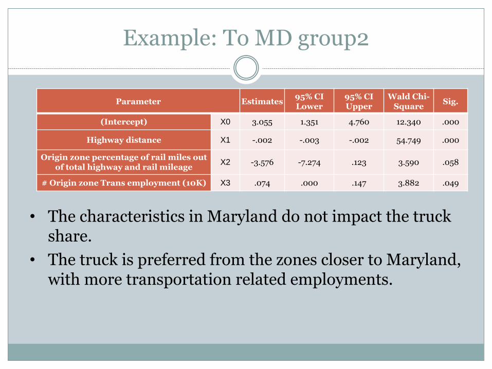
Example: To MD group2
• The characteristics in Maryland do not impact the truck share.
• The truck is preferred from the zones closer to Maryland, with more transportation related employments.
Parameter Estimates95% CI Lower
95% CI Upper
Wald Chi-Square
Sig.
(Intercept) X0 3.055 1.351 4.760 12.340 .000
Highway distance X1 -.002 -.003 -.002 54.749 .000
Origin zone percentage of rail miles out of total highway and rail mileage
X2 -3.576 -7.274 .123 3.590 .058
# Origin zone Trans employment (10K) X3 .074 .000 .147 3.882 .049

Choice Model for Rail
Parameter B
95% Wald Confidence
Interval
Hypothesis
Test
Lower Upper
Wald Chi-
Square
Group1
Commodity
from MD
(Intercept) 5.525 2.933 8.117 17.46
Truck_dist -0.001 -0.002 0 6.533
D_Port 0.29 -0.002 0.582 3.783
D_PAHwy_P -12.539 -17.422 -7.655 25.324
Group2
Commodity
from MD
(Intercept) 3.822 -0.862 8.506 2.557
Truck_dist -0.002 -0.003 -0.001 23.284
D_truck -0.228 -0.381 -0.075 8.536
D_PAHwy_P -14.252 -20.424 -8.08 20.486
Group1
Commodity to
MD
(Intercept) -2.339 -4.357 -0.32 5.158
Truck_dist -0.001 -0.002 0 6.233
O_truck -0.276 -0.461 -0.091 8.558
O_rail 0.155 0.101 0.209 31.586
D_TC_P -6.958 -12.129 -1.787 6.954
Group2
Commodity to
MD
(Intercept) 7.195 4.799 9.592 34.62
Truck_dist 0 -0.001 -6.50E-05 5.541
O_truck 0.127 0.008 0.246 4.349
O_rail 0.044 0.019 0.069 11.756
D_TC_P -2.173 -3.488 -0.858 10.495
D_RC_P -5.759 -8.147 -3.372 22.361
O_PAHwy_P -8.946 -12.704 -5.188 21.774

Sensitivity Analysis Results
Parameter 48 49 50
Group 1 from MD
# Origin zone truck center X2 1.2314 1.209 1.0761
# Origin zone rail center X3 0.9763 0.9783 0.9904
# Destination zone truck center X4 1.0545 1.0498 1.0213
# Destination zone rail center X5 0.9966 0.9969 0.9986
# Destination zone port center X6 1.0384 1.0351 1.0152
# Destination zone Trans
employment (10K)X7 0.9809 0.9825 0.9923
Group 2 from MD
# Destination zone rail center X2 0.9930 0.9931 0.9928
Destination zone principal
arterial percentage out of total
highway and rail mileage (1%)
X3 1.0115 1.0114 1.0120
# Destination zone Trans
employment (10K)X4 1.0352 1.0349 1.0366
Group 1 to MD
# Origin zone port related
distribution centerX2 0.9474 0.9713 0.9413
Destination zone rail center
percentage (1%)X3 0.9934 0.9964 0.9926
# Origin zone Trans employment
(10K)X4 1.0131 1.0069 1.0147
Group 2 to MD
Origin zone percentage of rail
miles out of total highway and
rail mileage (1%)
X2 0.9883 0.9883 0.9878
# Origin zone Trans employment
(10K)X3 1.0242 1.0240 1.0252

Summary
For Group 1 commodities, number of truck and rail centers will influence the percentage of tonnage carried by truck.
For Group 2 commodities, the percentage of truck tonnage only depends on the characteristics of the opposite zones.
The distance is a dominant variables related to truck share.
The principal arterial highway and rail coverage in the opposite zones are related to truck share for group 2, not group 1.
Number of transportation/warehousing employments in the opposite zones is significant.
Variables such as highway and rail coverage in MD and employment in MD is not related.

Potential Applications
Forecast of Future Freight Demand
Expansion of the Port of Baltimore
Expansion of Panama Canal and Northwest passage
Prevent Infrastructure Bottlenecks
Intermodal Facilities
Truck Distribution Centers
Economic Analysis
Project selection
Dollars lost by not providing infrastructure

Model Extensions

Overall contributing factors (1)

Overall contributing factors (2)

Differences Among Zones

Shipments from Zones
Chicago Freight Mode Choice Model78
Amir Samimia*, Kazuya Kawamurab and Abolfazl Mohammadian. (2011). A behavioral analysis of freight mode choice decisions. Transportation Planning and Technology, Vol. 34, No. 8, p. 857-869.

Data Collection79
Collected 881 domestic shipments in the United States.
A total of 4544 business establishments opened the recruiting email, of which 316 firms participated
A 7% response rate, which is a reasonable rate in such surveys.
Basic information about the following is obtained each establishment
five recent shipments, namely origin, destination, transportation mode, type, value, weight, and volume of the commodity
cost and time of the entire shipping process

Data-Descriptive Statistics80

Modeling Approach81
Used random utility maximization approach
Binary probit and logit
Goodness of fit
AIC
Log-likelihood
Rho-square
Sample validation for both modes
Predicted versus modeled

Model Results82

Marginal Effect and Elasticities83

London Freight Mode Choice Model84
Kriangkrai Arunotayanun , John W. Polak. (2011). Taste heterogeneity and market segmentation in freight shippers’ mode choice behaviour. Transportation Research Part E, 47, pp. 138-148.

Model Form85
MNL
Mixed MNL

Model Results86

Commodity Specific Mode Choice87

Sweden Freight Mode Choice Model88
Gerard de Jong , Moshe Ben-Akiva. (2007). A micro-simulation model of shipment size and transport chain choice, Transportation Research Part B 41, pp.950–965.

Model Summary89
Multinomial logit model for combined shipment size and mode choice
Weight choices
Up to 3500 kg
3501–15,000 kg
15,001–30,000 kg
30,001–100,000 kg
Above 100,000 kg
Nested and mixed models were not significant

Variables90

Results91