Lecture 1: Three Dimensional graphics: Projections and Transformations

Device Independence

Figure 1: Normalisation transformation

We will start with a brief discussion oftwo dimensional drawing primitives. Atthe lowest level of an operating sys-tem we have device dependent graphicsmethods such as:

SetPixel(XCoord,YCoord,Colour);DrawLine(xs,ys,xf,yf);

which draw objects using pixel coordi-nates. However it is clearly desirablethat we create any graphics applicationin a device independent way. If we cando this then we can re-size a picture, ortransport it to a different operating sys-tem and it will fit exactly in the windowwhere we place it. Many graphics APIsprovide this facility, and it is a straight-forward matter to implement it using a world coordinate system. This defines the coordinate values to beapplied to the window on the screen where the graphics image will be drawn. Typically it will use a method ofthe kind:

SetWindowCoords(Wxmin,Wymin,Wxmax,Wymax);WXMin etc are real numbers whose units are application dependent. If the application is to produce a visuali-sation of a house then the units could be meters, and if it is to draw accurate molecular models the units will beµm. The application program uses drawing primitives that work in these units, and converts the numeric valuesto pixels just before the image is rendered on the screen. This makes it easy to transport it to other systems orto upgrade it when new graphics hardware becomes available. There may be other device characteristics thatneed to be accounted for to achieve complete device independence, for example aspect ratios.

In order to implement a world coordinate system we need to be able to translate between world coordinatesand the device or pixel coordinates. However, we do not necessarily know what the pixel coordinates of awindow are, since the user can move and resize it without the program knowing. The first stage is therefore tofind out what the pixel coordinates of a window are, which is done using an enquiry procedure of the kind:

GetWindowPixelCoords(Dxmin, Dymin, Dxmax, Dymax)In the Windows API this procedure is called GetClientRect. Having established both the world and devicecoordinate systems, it is possible to define a normalisation process to compute the pixel coordinates from theworld coordinates. This is done by simple ratios as shown in Figure 1 . For the X direction:

(Xw −Wxmin)(Wxmax −Wxmin)

=(Xd −Dxmin)

(Dxmax −Dxmin)

Rearranging, and applying the same idea to the Y direction yields a pair of simple linear equations equations:

Xd = AXw +BYd = CYw +D

where the four constants A,B,C and D define the normalisation between the world coordinate system and thewindow pixel coordinates. Whenever a window is re-sized it is necessary to re-calculate the constants A,B,Cand D.

Graphical Input

The most important input device is the mouse, which records the distance moved in the X and Y directions. Inthe simplest form it provides at least three pieces of information: the x distance moved, the y distance movedand the button status. The mouse causes an interrupt every time it is moved, and it is up to the system software to

Interactive Computer Graphics Lecture 1 1

keep track of the changes. Note that the mouse is not connected with the screen in any way. Either the operatingsystem or the application program must achieve the connection by drawing the visible marker. The operatingsystem must share control of the mouse with the application, since it needs to act on mouse actions that takeplace outside the graphics window. For instance, processing a menu bar or launching a different application. Ittherefore traps all mouse events (ie changes in position or buttons) and informs the program whenever an eventhas taken place using a ”callback procedure”. The application program must, after every action carried out,return to the callback procedure (or event loop) to determine whether any mouse action (or other event such asa keystroke) has occurred. The callback is the main program part of any application, and, in simplified pseudocode, looks like this:

while (executing) do{ if (menu event) ProcessMenuRequest();

if (mouse event){ GetMouseCoordinates();

GetMouseButtons();PerformMouseProcess();}if (window resize event) RedrawGraphics();}

The procedure ProcessMenuRequest will be used to launch all the normal actions, such as save and open andquit, together with all the application specific requests. The procedures GetMouseCoordinates and Perform-MouseProcess will be used by the application writer to create whatever effect is wanted, for example, movingan object with the mouse. This may well involve re-drawing the graphics. If the window is re-sized then thewhole picture will be re-drawn.

3-Dimensional Objects Bounded by Planar Polygons (Facets)

Most graphical scenes are made up of planar facets. Each facet is an ordered set of 3D vertices, lying on oneplane, which form a closed polygon. The data describing a facet are of two types. First, there is the numericaldata which is a list of 3D points, (3 × N numbers for N points), and secondly, there is the topological datawhich describes how points are connected to form edges and facets.

Projections of Wire-Frame Models

Figure 2: Planar Projection

Since the display device is only 2D, we haveto define a transformation from the 3D spaceto the 2D surface of the display device. Thistransformation is called a projection. In gen-eral, projections transform an n-dimensionalspace into anm-dimensional space wherem <n. Projection of an object onto a surface isdone by selecting a viewpoint and then defin-ing projectors or lines which join each vertexof the object to the viewpoint. The projectedvertices are placed where the projectors inter-sect the projection surface as shown in Figure2.

The most common (and simplest) projections used for viewing 3D scenes use planes for the projectionsurface and straight lines for projectors. These are called planar geometric projections. A rectangular windowcan be defined defined on the plane of projection which can be mapped into the device window as describedabove. Once all the vertices of an object have been projected it can be rendered. An easy way to do this isdrawing all the projected edges. This is called a wire-frame representation. Note that for such rendering the

Interactive Computer Graphics Lecture 1 2

topological information only specifies which points are joined by edges. For other forms of rendering we alsoneed to define the object faces.

There are two common classes of planar geometric projections. Parallel projections use parallel projectors,perspective projections use projectors which pass through one single point called the viewpoint. In order tominimise confusion in dealing with a general projection problem, we can standardise the plane of projection bymaking it always parallel to the z = 0 plane, (the plane which contains the x and y axis). This does not limit thegenerality of our discussion because if the required projection plane is not parallel to the z = 0 plane then wecan use a coordinate transformations in 3D and make so. We will see shortly how to do this. We shall restrictthe viewed objects to be in the positive half space (z > 0), therefore the projectors starting at the vertices willalways run in the negative z direction.

Parallel Projections

Figure 3: Orthographic Projections

In a parallel projection all the projectors have the same direction d,and the viewpoint can be considered to be at infinity. For a vertexV = [Vx, Vy, Vz] the projector is defined by the parametric line equa-tion:

P = V + µdIn orthographic projection the projectors are perpendicular to the projec-tion plane, which we usually define as z = 0. In this case the projectorsare in the direction of the z axis and:

d = [0, 0,−1]and so Px = Vx

and Py = Vy

which means that the x and y co-ordinates of the projected vertex areequal to the x and y co-ordinates of the vertex itself and no calculations are necessary. Some examples of awireframe cube drawn in orthographic projection are shown in Figure 3.

If the projectors are not perpendicular to the plane of projection then the projection is called oblique. Theprojected vertex intersects the z = 0 plane where the z component of the P vector is equal to zero, therefore:

Pz = 0 = Vz + µdz

so µ = −Vz/dz

and we can use this value of µ to compute:Px = Vx + µdx = Vx − dxVz/dz

and Py = Vy + µdy = Vy − dyVz/dz

These projections are similar to the orthographic projection with one or other of the dimensions scaled. Theyare not often used in practice.

Perspective Projections

In perspective projection, all the rays pass through one point in space, the centre of projection as shown infigure 2. If the centre of projection is behind the plane of projection then the orientation of the image is thesame as the 3D object. By contrast, in a pin hole camera it is inverted. To calculate perspective projections weadopt a canonical form in which the centre of projection is at the origin, and the projection plane is placed at aconstant z value, z = f . This canonical form is illustrated in Figure 4. The projection of a 3D point onto thez = f plane is calculated as follows. If we are projecting the point V then the projector has equation:

P = µVSince the projection plane has equation z = f , it follows that, at the point of intersection:

f = µVz

If we write µp = f/Vz for the intersection point on the plane of projection then:Px = µpVx = fVx/Vz

and Py = µpVy = fVy/Vz

Interactive Computer Graphics Lecture 1 3

The factor µp is called the foreshortening factor, because the further away an object is, the larger Vz and thesmaller is its image. Some examples of the perspective projection of a cube are shown in figure 5.

Figure 4: Canonical form for perspective projection Figure 5: Perspective projection of a cube

Space Transformations

The introduction of canonical forms for perspective and orthographic projection simplifies their computation.However, in cases where we wish to move around a graphical scene and view if from any particular point, wemust be able to transform the coordinates of the scene, such that the view direction is along the z axis and(for perspective projection) the viewpoint is at the origin. In general we would like to change the coordinatesof every point in the scene, such that some chosen viewpoint C = [Cx, Cy, Cz] is the origin and some viewdirection d = [dx, dy, dz] is the Z axis. This new coordinate system in which the scene is to be defined issometimes called the “view centered” coordinate system and is shown in Figure 6.

Figure 6: View centered coordinate transformation

Frequently, we may also want to transform the points of a graphical scene for other purposes such asgeneration of special effects like rotating or shrinking objects. Transformations of this kind are achieved bymultiplying every point of the scene by a transformation matrix. Unfortunately however, we cannot perform ageneral translation using normal Cartesian coordinates, and for that reason we now introduce a system calledhomogeneous coordinates. Three dimensional points expressed in homogeneous form have a fourth ordinate:

P = [px, py, pz, s]The fourth ordinate is a scale factor, and conversion to Cartesian form is achieved by dividing it into the otherordinates, so:

[px, py, pz, s] has Cartesian coordinate equivalent [px/s, py/s, pz/s]In most cases s will be 1. The point of introducing homogenous coordinates is to allow us to translate the points

Interactive Computer Graphics Lecture 1 4

of a scene by using matrix multiplication.

[x, y, z, 1]

1 0 0 00 1 0 00 0 1 0tx ty tz 1

= [x+ tx, y + ty, x+ tz, 1]

The matrix for scaling a graphical scene is also easily expressed in homogenous form:

[x, y, z, 1]

sx 0 0 00 sy 0 00 0 sz 00 0 0 1

= [sxx, syy, szz, 1]

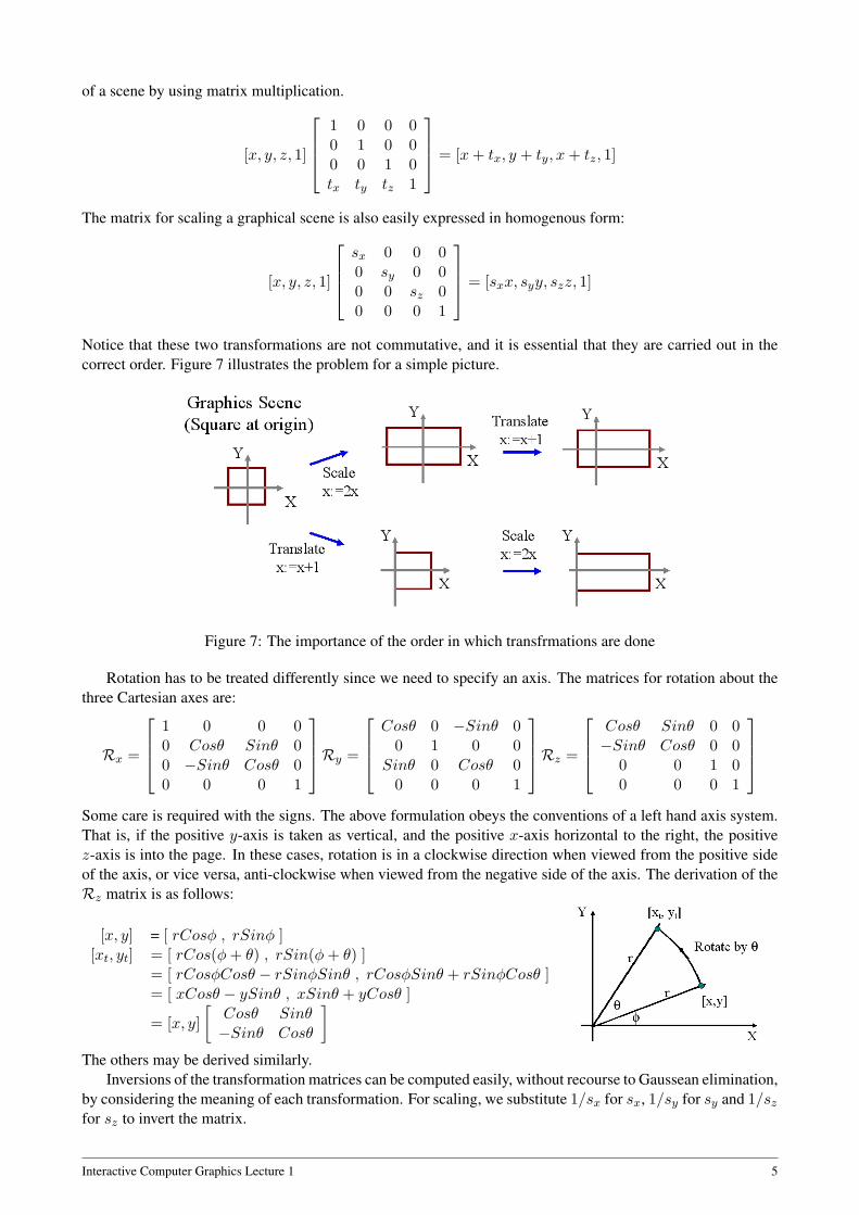
Notice that these two transformations are not commutative, and it is essential that they are carried out in thecorrect order. Figure 7 illustrates the problem for a simple picture.

Figure 7: The importance of the order in which transfrmations are done

Rotation has to be treated differently since we need to specify an axis. The matrices for rotation about thethree Cartesian axes are:

Rx =

1 0 0 00 Cosθ Sinθ 00 −Sinθ Cosθ 00 0 0 1

Ry =

Cosθ 0 −Sinθ 0

0 1 0 0Sinθ 0 Cosθ 0

0 0 0 1

Rz =

Cosθ Sinθ 0 0−Sinθ Cosθ 0 0

0 0 1 00 0 0 1

Some care is required with the signs. The above formulation obeys the conventions of a left hand axis system.That is, if the positive y-axis is taken as vertical, and the positive x-axis horizontal to the right, the positivez-axis is into the page. In these cases, rotation is in a clockwise direction when viewed from the positive sideof the axis, or vice versa, anti-clockwise when viewed from the negative side of the axis. The derivation of theRz matrix is as follows:

[x, y] = [ rCosφ , rSinφ ][xt, yt] = [ rCos(φ+ θ) , rSin(φ+ θ) ]

= [ rCosφCosθ − rSinφSinθ , rCosφSinθ + rSinφCosθ ]= [ xCosθ − ySinθ , xSinθ + yCosθ ]

= [x, y][

Cosθ Sinθ−Sinθ Cosθ

]The others may be derived similarly.

Inversions of the transformation matrices can be computed easily, without recourse to Gaussean elimination,by considering the meaning of each transformation. For scaling, we substitute 1/sx for sx, 1/sy for sy and 1/sz

for sz to invert the matrix.

Interactive Computer Graphics Lecture 1 5

sx 0 0 00 sy 0 00 0 sz 00 0 0 1

has inversion

1/sx 0 0 0

0 1/sy 0 00 0 1/sz 00 0 0 1

For translation we substitute −tx for tx, −ty for ty and −tz for tz .

1 0 0 00 1 0 00 0 1 0tx ty tz 1

has inversion

1 0 0 00 1 0 00 0 1 0−tx −ty −tz 1

For the rotation matrices we note that:

Cos(−θ) = Cos(θ) and Sin(−θ) = −Sin(θ)

Hence to invert the matrix we simply change the sign of the Sin terms, for example:Cosθ Sinθ 0 0−Sinθ Cosθ 0 0

0 0 1 00 0 0 1

has inversion

Cosθ −Sinθ 0 0Sinθ Cosθ 0 0

0 0 1 00 0 0 1

Interactive Computer Graphics Lecture 1 6

Lecture 2: Scene Transformation and Animation

Flying Sequences

We will now consider a most important subject, namely, scene transformation. In any viewer centered appli-cation, such as a flight simulator or a computer game, we need to view the scene from a moving position. Asthe viewpoint changes we transform all the coordinates of the scene such that the viewpoint is the origin andthe view direction is the z axis, before projecting and drawing the scene. Let us suppose that, in the coordinatesystem in which the scene is defined we wish to view it from the point C = [Cx, Cy, Cz], looking along thedirection d = [dx, dy, dz]. The first step is to move the origin to C for which we use the transformation matrixA.

A =

1 0 0 00 1 0 00 0 1 0−Cx −Cy −Cz 1

Following this, we wish to rotate about the y-axis so that d lies in the plane x = 0. Using the fact that d isdefined by the co-ordinates [dxdydz] and using the notation v2 = d2

x + d2z this is done by matrix B.

v =√d2

x + d2z

Cosθ = dz/v

Sinθ = dx/v

B =

dz/v 0 dx/v 0

0 1 0 0−dx/v 0 dz/v 0

0 0 0 1

Notice that we have avoided computing the Cos and Sin functions for this rotation by use of the directioncosine. To get the direction vector lying along the z axis a further rotation is needed. This time it is about the xaxis using matrix C.

v =√d2

x + d2z

Cosφ = v/|d|

Sinφ = dy/|d|

C =

1 0 0 00 v/|d| dy/|d| 00 −dy/|d| v/|d| 00 0 0 1

Finally the transformation matrices are combined into one, and each point of the scene is transformed:T = A · B · C

and so for all the pointsPt = P · T

Problems with verticals

Figure 1: Inversion of the Vertical

The concept of “vertical” is missing from the above anal-ysis, and needs attention since it is easy to invert the ver-tical. This will be easily observed in the trivial exampleof figure 1, where an arrow whose base is at [0,0,-l] isbeing observed from the origin. A transformation basedon rotating about the y axis first yields the correct solu-tion. However, a transformation involving rotation aboutthe x axis first inverts the image.

Interactive Computer Graphics Lecture 2 1

Rotation about a general line

A very similar problem to the viewer centered transformation concerns animation of objects in a fixed scene.Let us suppose that we want to rotate one sub-object about some line in the Cartesian space where the scene isdefined. Let the line be: L + µd where L = [Lx, Ly, Lz] is the position vector of any point on the line and dis a unit direction vector along the line. We use a translation to move the origin so that it is on the line (matrixA but transforming the origin to L rather than C) followed by two rotations to make the z axis coincident withthe direction vector d (matrices B and C). Now we can perform a rotation of the object about the z-axis usingthe standard rotation matrix Rz defined previously. Finally we need to restore the coordinate system as it was,such that the viewpoint is the same as before. To do this we simply invert the transformation matrices A B andC. As before we multiply all the individual transformation matrices together to make one matrix which is thenapplied to all the points.T = A · B · C · Rz · C−1 · B−1 · A−1

and for all the points Pt = P · TOther object transformations for graphical animation are performed similarly. For example to make an

object shrink we move the origin to its centre, perform a scaling and then restore the origin to its originalposition.

Projection by Matrix Multiplication

If we use homogeneous co-ordinates then it is also possible to compute projection by multiplication by aprojection matrix. Placing the centre of projection at the origin and using z = f as the projection plane givesus matrixMp for perspective projection. MatrixMo is for orthographic projection:

Mp =

1 0 0 00 1 0 00 0 1 1/f0 0 0 0

Mo =

1 0 0 00 1 0 00 0 0 00 0 0 1

It is not immediately obvious that matrixMp produces the correct perspective projection. Let us transform anarbitrary point V with homogeneous co-ordinates [x, y, z, 1] by using matrix multiplication. For the projectedpoint P we get:

P = V · Mp = [x, y, z, z/f ]

This point must be normalised into a Cartesian coordinate. To do this we divide the first three co-ordinates bythe value of the fourth and we get:

Pc = [xf/z, yf/z, f, 1]

which is the projected point. It is interesting to note that the projection matrix is obviously singular (it has a rowof zeros) and, therefore, it has no inverse. This must be so because it is impossible to reconstruct a 3D objectfrom its 2D projection without other information. Projection matrices can of course be combined with the othermatrices. Indeed the popularity of the orthographic projection is that it simplifies the amount of calculationssince the z row and column fall to zero. Although a simplification applies when the perspective projection isused, there is also the need to normalise the resulting homogenous coordinates, and this adds to the computationtime.

Homogenous coordinates

We now take a second look at homogeneous coordinates, and their relation to vectors. Previously, we describedthe fourth ordinate as a scale factor, and ensured that, with the exception of the projection transformation, itwas always normalised to 1. As an alternative, we can consider the fourth ordinate as indicating a type asfollows. Informally we acknowledge that a normal Cartesian coordinate is a special form of vector, which wecall a position vector, and usually denote using bold face capital letters. Hence, we can say that a normalisedhomogenous coordinate is the same as a position vector.

By contrast, if we consider a homogenous coordinate where the last ordinate is zero - [x, y, z, 0] - we findthat we cannot normalise it in the usual way because of the divide by zero. So clearly a homogenous coordinateof this form cannot be directly associated with a point in Cartesian space. However, it still has a magnitude and

Interactive Computer Graphics Lecture 2 2

direction, and hence we can consider it to be a direction vector. Thus homogenous coordinates fall into twoclasses, those with the final ordinate non-zero, which can be normalised into position vectors or points, andthose with zero in the final ordinate which are direction vectors, or vectors in the pure sense of the word.

Figure 2: Definition of a straight line

Consider now how vector addition works with these definitions.If we add two direction vectors, we add the ordinates as before andwe obtain a direction vector. ie:

[xi, yi, zi, 0] + [xj , yj , zj , 0] = [xi + xj , yi + yj , zi + zj , 0]

This is the normal vector addition rule which operates independentlyof Cartesian space. However, if we add a direction vector to a positionvector we obtain a position vector or point:

[Xi, Yi, Zi, 1] + [xj , yj , zj , 0] = [Xi + xj , Yi + yj , Zi + zj , 1]

This is a nice result, because it ties in with our definition of a straightline in Cartesian space, which is the sum of a point and a scaled di-rection as shown in figure 2.

Now, consider a general affine transformation matrix. We ignore the possibility of doing perspective pro-jection or shear, so that the last column will always be [0, 0, 0, 1]T , and the matrix will be of the form shown infigure 3, with the rows viewed as three direction vectors and a position vector.

Figure 3: The structure of a space transformation matrix

To see what the individual rows mean we consider the effect of the transformation in simple cases. Forexample take the unit vectors along the Cartesian axes eg i = [1, 0, 0, 0]:

[1, 0, 0, 0]

qx qy qz 0rx ry rz 0sx sy sz 0Cx Cy Cz 1

= [qx, qy, qz, 0]

In other words the direction vector of the top row represents the direction in which the x axis points aftertransformation, and similarly we find that j = [0, 1, 0, 0] will be transformed to direction [rx, ry, rz, 0] and k =[0, 0, 1, 0] will be transformed to [sx, sy, sz, 0]. Similarly, we can see the effect of the bottom row by consideringthe transformation of the origin which has homogeneous coordinate [0, 0, 0, 1]. This will be transformed to[Cx,Cy,Cz, 1].

[0, 0, 0, 1]

qx qy qz 0rx ry rz 0sx sy sz 0Cx Cy Cz 1

= [Cx, Cy, Cz, 1]

Notice also that the zero in the last ordinate ensures that direction vectors will not be affected by thetranslation, whereas all position vectors will be moved by the same factor. Notice also that if we do not shearthe object the three vectors q r and s will remain orthogonal so that q · r = r · s = q · s = 0. Unfortunatelyhowever, this analysis does not help us to determine the transformation matrix, though we will need it laterin the course when we look at annimation. In general it would be more natural to assume that we know thevectors u,v, and w which form the view centered coordinate system. To see how to write down a transformationmatrix from thses vectors we need to introduce the notion of the dot product as a projection onto a line. This ismost readily seen in two dimensions as shown in Figure 4. By dropping perpendiculars from the point P to theline defined by vector u and vector v we see that the distances from the origin are respectively P · u and P · v.

Interactive Computer Graphics Lecture 2 3

Figure 4: The dot product as projectionFigure 5: Three dimensional point projection

P · u = |P||u|Cosθ = |P|Cosθ since u is a unit vector. Now, suppose that we wish to rotate the scene so thatthe new x and y axes were the u and v vectors, then the x ordinate would be defined by P ·u and the y by P · v.

The generalisation to three dimensions is shown in figure 5, in which a point P is transformed into the(u, v, w) axis system, translated by vector C, is given by:

P tx = (P−C) · uP t

y = (P−C) · vP t

z = (P−C) · wExpressing this as a transformation matrix we get:

[P tx, P

ty, P

tz , 1] = [Px, Py, Pz, 1]

ux vx wx 0uy vy wy 0uz vz wz 0−C · u −C · v −C · w 1

So now by maintaining values of u, v, w and w throughout an animation sequence, for example by adjusting theirvalues in response to mouse or joystick commands, we can simply write down the correct scene transformationmatrix for viewing the virtual world from the correct position.

Finally we will derive the matrix used for a view centered transformation with the viewer at point C andlooking in direction d by finding the new axis system u, v, w, and then deducing the transformation matrix.The direction vector for viewing is d = [dx, dy, dz] and this must lie along the w direction, so w = d/|d|. Wefirst find any two vectors, p and q,which have the same directions as u and v, but do not necessarily have unitlength. We can constrain the system to preserve horizontals and verticals in two ways: (i) Vector p will be inthe direction of the new x-axis, so to preserve the horizontal, we choose: py = 0, and (ii) Vector q will be thenew y axis (vertical) and should have a positive y component (so that the picture is not upside down) so wechoose (arbitrarily): qy = 1. Substituting our constraints in the Cartesian components we get:

p = [px, 0, pz] and q = [qx, 1, qz]Now we know that, in a left hand axis system:

k = i× j so therefore we can write: d = p× qsince we have not as yet constrained the magnitude of p. Evaluating the cross product we get three Cartesianequations:

dx = pyqz − pzqy dy = pzqx − pxqz dz = pxqy − pyqxSubstituting the values py = 0 and qy = 1 these equations simplify to

dx = −pz dy = pzqx − pxqz dz = px

Thus we have solved for vector p = [dz, 0,−dx]. To solve for q we need to express the condition that p and qare orthogonal and so have zero dot product, whence:

p · q = dzqx + 0− dxqz = 0 thus qz = dzqx/dx

and from the cross product already evaluated:dy = pzqx − pxqz = −dxqx − dzqz = −dxqx − d2

zqx/dx

so qx = −dydx/(d2x + d2

z)and q = (−dydx/(d2

x + d2z), 1, dydz/(d2

x + d2z))

finally we have that: u = p/|p| and v = q/|q|Thus we can deduce the whole of the transformation matrix.

Interactive Computer Graphics Lecture 2 4

DOC Interactive Computer Graphics Tutorial 1 page 1

Tutorial 1: Analysis of three dimensional space. This tutorial is about the use of vector algebra in the analysis of three dimensional scenes used in computer graphics system. The following notation is used:

• Position vectors are denoted by boldface capital letters: P, Q, V etc. Position vectors are the same as cartesian coordinates, and represent position relative to the origin.

• Direction vectors are indicated by boldface lowercase letters d, n etc. Direction vectors are independent of any origin.

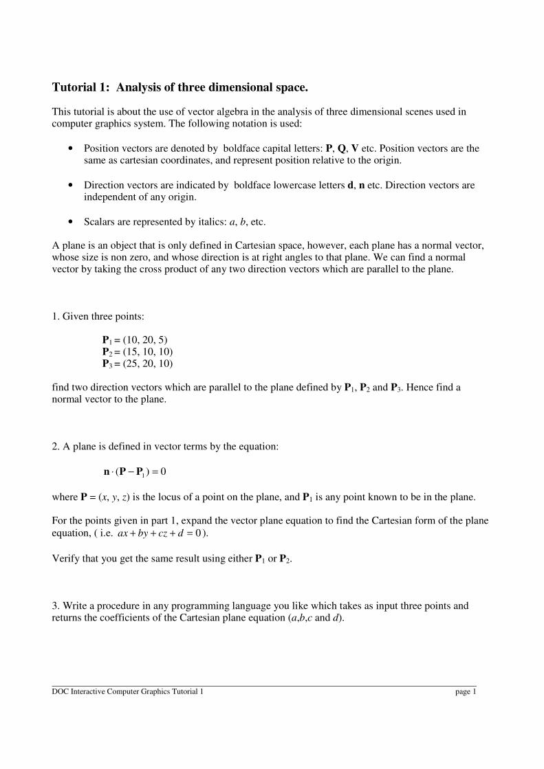
• Scalars are represented by italics: a, b, etc. A plane is an object that is only defined in Cartesian space, however, each plane has a normal vector, whose size is non zero, and whose direction is at right angles to that plane. We can find a normal vector by taking the cross product of any two direction vectors which are parallel to the plane. 1. Given three points:

P1 = (10, 20, 5) P2 = (15, 10, 10) P3 = (25, 20, 10)

find two direction vectors which are parallel to the plane defined by P1, P2 and P3. Hence find a normal vector to the plane. 2. A plane is defined in vector terms by the equation:

0)( 1 =−⋅ PPn

where P = (x, y, z) is the locus of a point on the plane, and P1 is any point known to be in the plane. For the points given in part 1, expand the vector plane equation to find the Cartesian form of the plane

equation, ( i.e. 0=+++ dczbyax ).

Verify that you get the same result using either P1 or P2. 3. Write a procedure in any programming language you like which takes as input three points and returns the coefficients of the Cartesian plane equation (a,b,c and d).

DOC Interactive Computer Graphics Tutorial 1 page 2

4. Starting from any point on a face of a polyhedron, an inner surface normal is a normal vector to the plane of the face whose direction points into the polyhedron. A tetrahedron is defined by the three points of part 1, and a fourth point P4 = (30, 20, 10). Determine whether the normal vector that you calculated in part 1 is an inner surface normal, and if not find the inner surface normal. 5. Two lines intersect at a point P1, and are in the directions defined by d1 and d2. Provided that d1 and d2 represent different directions, the two lines define a plane.

Any point on the plane can be reached by travelling from P1 in direction d1 by some distance µ and

then in direction d2 by a distance ν.

Using this fact construct the parametric equation of any point on the plane of part 1 in terms of µ,ν, P1, P2 and P3. By taking the dot product with a normal vector to the plane n, show that the parametric plane equation is equivalent to the vector plane equation of part 2.

Vector Algebra Revision Notes

A vector is a one dimensional array of numbers: [1,55,79.3, -25] is a vector. For analysis of three dimensionalgeometry we will consider only vectors of dimension two or three.

A vector p = [px, py, pz] has magnitude computed by |p| =√

(p2x + p2

y + p2z) and a direction which is

defined by angles with the Cartesian axes: θx, θy, θz where cos θx = px/|p|, cos θy = py/|p| and cos θz =pz/|p|. A vector does not have any particular position on the Cartesian axes.

A unit vector is one where |p| = 1. By convention, the unit vectors in the directions of the Cartesian axesare labelled i = [1, 0, 0], j = [0, 1, 0] and k = [0, 0, 1]. Unit vectors are often used for specifying directions.Lower case bold italic letters are used for unit vectors in these notes.

A position vector is simply a coordinate in Cartesian space. It is a particular instance of a vector whichstarts from the origin. Upper case bold letters are used for position vectors in these notes.

A direction vector is the same as a vector. The name is used particularly when a vector defines a directionand its magnitude is not relevant. Lower case bold letters are used for direction vectors in these notes.

Vector Addition: There is only one way to add vectors, and that is to add the individual ordinates, so:p + q = [px, py, pz] + [qx, qy, qz] = [px + qx, py + qy, pz + qz].

Scalar multiplication: Multiplication of a vector by a scalar means that each element of the vector ismultiplied by the scalar, ie µd = µ[dx, dy, dz] = [µdx, µdy, µdz]. Multiplication by −1 reverses the directionof a vector. Scalar multiplication and vector addition can be combined to define a line in Cartesian space. Theequation: P = B+µd specifies a line through point (position vector) B in direction d. Choosing any value ofµ will identify one point on the line.

The scalar (or dot) product: There are two ways of multiplying two vectors together. The scalar productreturns a scalar value defined as p · q = pxqx + pyqy + pzqz . Note that we can write the magnitude of a vectoras |p| =

√(p · p). The dot product can be written equivalently as p · q = |p||q| cos(θ) where θ is the angle

between the directions of p and q. The dot product has some useful properties:

1. If two vectors are at right angles, the dot product is zero.

2. If the angle between two vectors is acute the dot product is positive.

3. If one of the vectors is a unit vector the dot product is a projection of the other vector in that direction.

The vector (or cross) product: The second way of multiplying two vectors results in a vector defined by:p×q = [(pyqz−pzqy), (pzqx−pxqz), (pxqy−pyqx)]. This formula may be easily remembered by consideringthe evaluation of the determinant:

p× q =i j kpx py pz

qx qy qz

The vector product is a vector whose magnitude is given by p×q = |p||q| sin(θ) and whose direction is at rightangles to both p and q. Note that p×p = [0, 0, 0] and has no direction. The same is true for any two vectors withthe same direction. To be precise about the direction we need to know its sign. The rule for determining this isbest remembered by thinking of the two vectors as the hands of a clock. Measuring the angle clockwise from pto q the direction is into the clock for positive |p||q| sin(θ). Note that p×q = −q×p since, if the angle betweenp and q is θ, then the angle between q and p will be sin(360 − θ), and sin(360 − θ) = sin(−θ) = − sin(θ).The useful property of the cross product is that it defines a direction at right angles to two vectors. Thus we canuse it to find the normal vector to a plane simply by taking the cross product of two vectors on the plane. Formost graphics applications we need to test which direction the normal vector goes.

Interactive Computer Graphics :Vector Algebra Revision Notes 1