Lecture 1, Jan 19

Review of the expected value, covariance, correlation coefficient, mean, andvariance.

Random variable. A variable that takes on alternative values according tochance. More specifically, a random variable assumes different values, eachwith probability less than or equal to 1.

A continuous random variable may take on any value on the real numberline. A discrete random variable may take only a specific number of values.

Probability mass function (pmf) and probability density function(pdf). The process that generates the values of a random variable. It listsall possible outcomes and the probability that each will occur.

Expected values. The mean, or the expected value, of a random variableX is a weighted average of the possible outcomes, where the probabilities ofthe outcomes serve as the weights. Expectation operator denoted E, meanof X denoted µX . In the discrete case,

µX = E(X) = p1X1 + p2X2 + · · ·+ pNXN =N∑

i=1

piXi,

where pi = P (X = Xi) and∑N

i=1 pi = 1.

In the continuous case, µX = E(X) =∫Ω f(x)xdx, where Ω is the support

of X, and f(x) is the pdf of X.

The sample mean of a set of outcomes on X is denoted by X.

X =1

n

n∑

i=1

xi,

where x1, . . . , xn are realizations of X.

1

Variance. The variance of a random variable provides a measure of thespread, or dispersion, around the mean. Var(X) = σ2

X = E[X − E(X)]2. Inthe discrete case,

Var(X) = σ2X =

N∑

i=1

pi[Xi − E(X)]2.

The positive square root of the variance is called the standard deviation.

Joint distribution. In the discrete case, joint distributions of X and Y aredescribed by a list of probabilities of occurrence of all possible outcomes onboth X and Y .

The covariance of X and Y is Cov(X,Y ) = E[X − E(X)(Y − E(Y )].In the discrete case,

Cov(X,Y ) = pij

N∑

i=1

M∑

j=1

[Xi − E(X)][Yj − E(Y )],

where pij represents the joint probability of X = Xi and Y = Yj occurring.

The covariance is a measure of the linear association between X and Y .If both variables are always above and below their means at the same time,the covariance will be positive. If X is above its mean when Y is below itsmean and vice versa, the covariance will be negative.

The value of covariance depends upon the units in which X and Y aremeasured. The correlation coefficient ρXY is a measure of the associationwhich has been normalized and is scale-free.

ρXY =Cov(X, Y)

σXσY

,

where σX and σY represent the standard deviation of X and Y respectively.The correlation coefficient is always between -1 and 1. A positive correlationindicates that the variables move in the same direction, while a negativecorrelation implies that they move in opposite directions.

Properties. Suppose X and Y are random variables, a and b are constants:

1. E(aX + bY ) = aE(X) + bE(Y );

2. Var(aX + b) = a2Var(X);

3. Var(X + Y ) = Var(X) + Var(Y ) + 2Cov(X,Y );

4. If X and Y are independent, then Cov(X,Y ) = 0.

2

Estimation.

Means, variances and covariances can be measured with certainty only if weknow all there is to know about all possible outcomes. In practice, we mayobtain a sample of the relevant information needed. Given x1, . . . , xn arerandom observations of X, we want to estimate a population parameter (likethe mean or the variance).

The sample mean X is an unbiased estimator of the population mean µX .

E(X) = E(1

n

n∑

i=1

xi) =1

n

n∑

i=1

E(xi) =1

n

n∑

i=1

µX = µX .

The sample variance s2X = 1

n−1

∑ni=1(xi− X)2 is an unbiased estimator of

the population variance Var(X).

The sample covariance sXY = 1n−1

∑ni=1(xi − X)(yi − Y ) is an unbiased

estimator of the population covariance Cov(X,Y ).

The sample correlation coefficient is defined as

rXY =

∑ni=1(xi − X)(yi − Y )√∑n

i=1(xi − X)2∑n

i=1(yi − Y )2.

Desired properties of estimators:

1. Lack of bias. The bias associated with an estimated parameter is de-fined to be: Bias(β) = E(β)−β. β is an unbiased estimator if the meanor the expected value of β is equal to the true value, that is, E(β) = β.

2. Consistency. β is an consistent estimator of β if for any δ > 0,lim

n→∞P (|β − β| < δ) = 1. As sample size n approaches infinity, the

probability that β will differ from β will get very small.

3. Efficiency. We say that β is an efficient unbiased estimator if for agiven sample size, the variance of β is smaller than the variance of anyother unbiased estimators.

3

Lecture 2, Jan 26

Tradeoff between bias and variance of estimators. When the goal isto maximize the precision of the predictions, an estimator with low varianceand some bias may be more desirable than an unbiased estimator with highvariance. We may want to minimize the mean square error, defined as

Mean square error(β) = E(β − β)2.

It can be shown that Mean square error(β) = [Bias(β)]2 +Var(β). The crite-rion of minimizing mean square error take into account of both the varianceand the bias of the estimator.

An alternative criterion to consistency is that the mean square error ofthe estimator approaches zero as the sample size increases. This impliesasymptotically, or when the sample size is very large, the estimator is unbi-ased and its variance goes to zero. An estimator with a mean square errorthat approaches zero will be consistent estimator but that the reverse need notbe true.

1

Probability distributions.

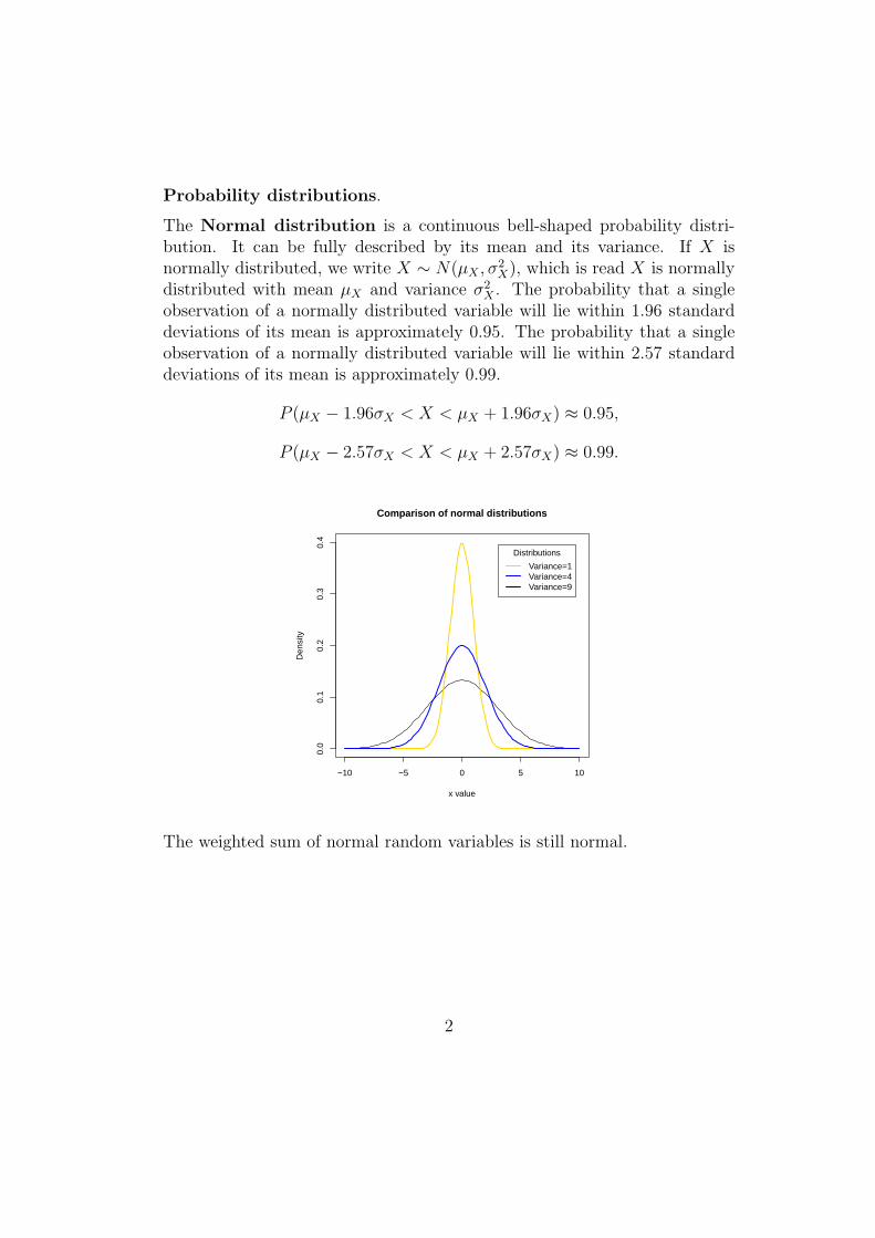
The Normal distribution is a continuous bell-shaped probability distri-bution. It can be fully described by its mean and its variance. If X isnormally distributed, we write X ∼ N(µX , σ2

X), which is read X is normallydistributed with mean µX and variance σ2

X . The probability that a singleobservation of a normally distributed variable will lie within 1.96 standarddeviations of its mean is approximately 0.95. The probability that a singleobservation of a normally distributed variable will lie within 2.57 standarddeviations of its mean is approximately 0.99.

P (µX − 1.96σX < X < µX + 1.96σX) ≈ 0.95,

P (µX − 2.57σX < X < µX + 2.57σX) ≈ 0.99.

−10 −5 0 5 10

0.0

0.1

0.2

0.3

0.4

Comparison of normal distributions

x value

Den

sity

Distributions

Variance=1Variance=4Variance=9

The weighted sum of normal random variables is still normal.

2

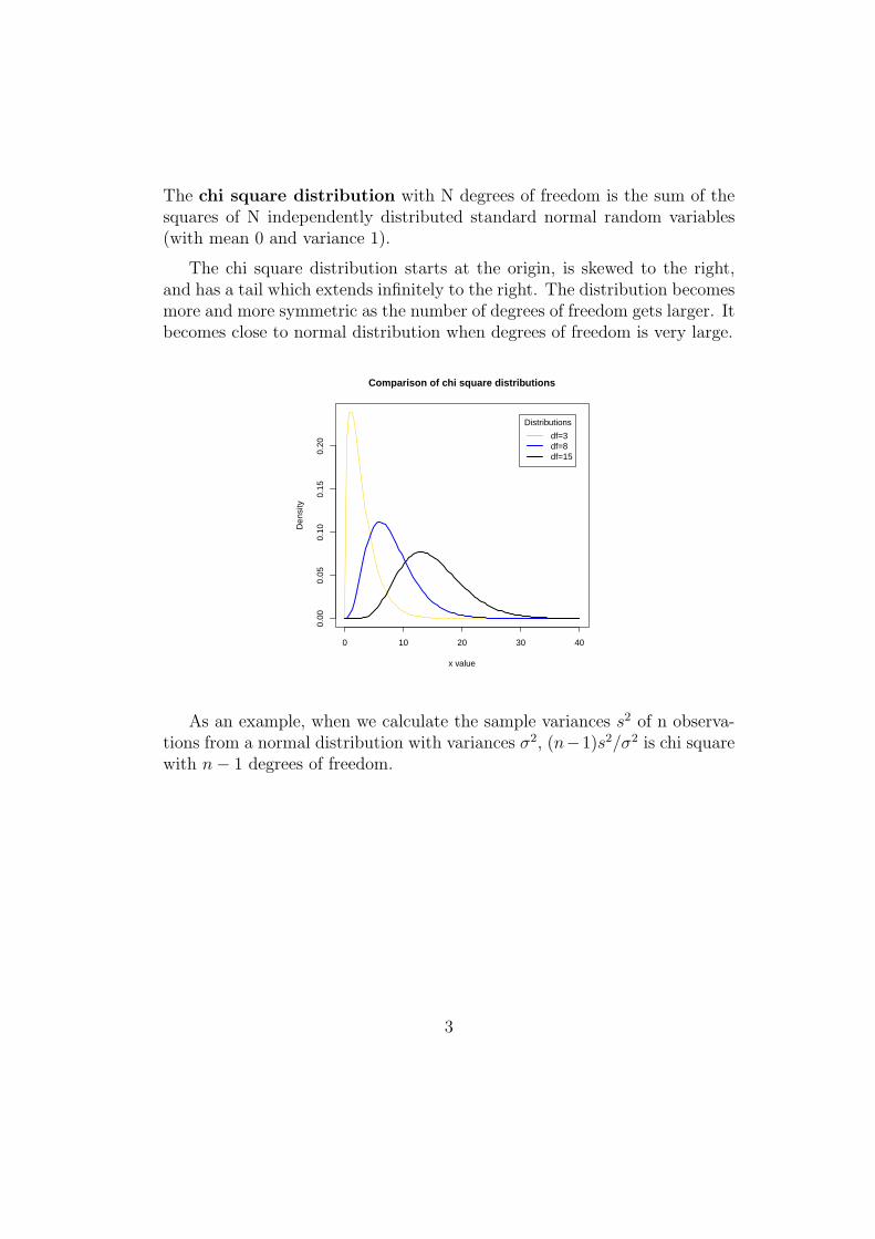
The chi square distribution with N degrees of freedom is the sum of thesquares of N independently distributed standard normal random variables(with mean 0 and variance 1).

The chi square distribution starts at the origin, is skewed to the right,and has a tail which extends infinitely to the right. The distribution becomesmore and more symmetric as the number of degrees of freedom gets larger. Itbecomes close to normal distribution when degrees of freedom is very large.

0 10 20 30 40

0.00

0.05

0.10

0.15

0.20

Comparison of chi square distributions

x value

Den

sity

Distributions

df=3df=8df=15

As an example, when we calculate the sample variances s2 of n observa-tions from a normal distribution with variances σ2, (n−1)s2/σ2 is chi squarewith n− 1 degrees of freedom.

3

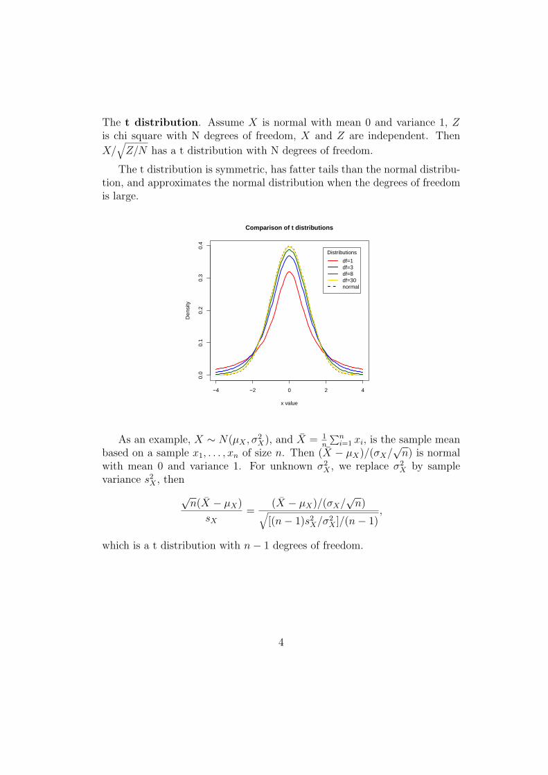
The t distribution. Assume X is normal with mean 0 and variance 1, Zis chi square with N degrees of freedom, X and Z are independent. Then

X/√

Z/N has a t distribution with N degrees of freedom.

The t distribution is symmetric, has fatter tails than the normal distribu-tion, and approximates the normal distribution when the degrees of freedomis large.

−4 −2 0 2 4

0.0

0.1

0.2

0.3

0.4

Comparison of t distributions

x value

Den

sity

Distributions

df=1df=3df=8df=30normal

As an example, X ∼ N(µX , σ2X), and X = 1

n

∑ni=1 xi, is the sample mean

based on a sample x1, . . . , xn of size n. Then (X − µX)/(σX/√

n) is normalwith mean 0 and variance 1. For unknown σ2

X , we replace σ2X by sample

variance s2X , then

√n(X − µX)

sX

=(X − µX)/(σX/

√n)√

[(n− 1)s2X/σ2

X ]/(n− 1),

which is a t distribution with n− 1 degrees of freedom.

4

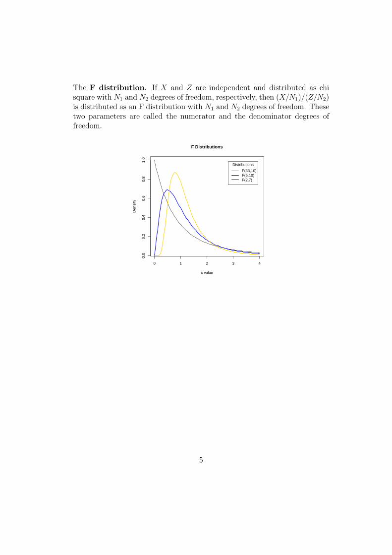
The F distribution. If X and Z are independent and distributed as chisquare with N1 and N2 degrees of freedom, respectively, then (X/N1)/(Z/N2)is distributed as an F distribution with N1 and N2 degrees of freedom. Thesetwo parameters are called the numerator and the denominator degrees offreedom.

0 1 2 3 4

0.0

0.2

0.4

0.6

0.8

1.0

F Distributions

x value

Den

sity

Distributions

F(33,10)F(5,10)F(2,7)

5

Forecasting: to calculate or predict some future event or condition, usuallyas a result of rational study or analysis of pertinent data.

We all make forecasts: a person waiting for a bus; parents expecting a tele-phone call from their children; bank manager predicts cash flow for the nextquarter; company manager predicts sales or estimates number of man-hoursrequired to meet a given production schedule.

Future events involve uncertainty. Forecasts are not perfect. The objectiveof forecasting is to reduce the forecast error. Each forecast has its ownspecifications, and solutions to one are not solutions in another situation.

General principles for any forecast system:Model specification; Model estimation; Diagnostic checking; Forecast gener-ation; Stability checking; Forecast updating.

Choice of forecast model. (1) Degrees of accuracy required; (2) forecasthorizon; (3) budget; (4) what data is available. One may not constructaccurate empirical forecast models from limited and incomplete data base.

Forecast criteria. Actual observation at time t is zt. Its forecast, whichuses the information up to and including time t− 1, is zt−1(1). Objective isto make the future forecast error zt − zt−1(1) as small as possible. However,zt is unknown, we can only talk about its expected value, conditional on theobserved data up to and including time t−1. We minimize the mean absoluteerror E|zt − zt−1(1)| or the mean square error E[zt − zt−1(1)]2. We use themean square error criterion for simpler mathematical calculations.

What we will discuss. In single-variable forecasting, we use past historyof the series, zt, where t is the time index, to extrapolate into the future.In regression forecasting, we use the relationships between the variable to beforecast and the other variables.

In the most general form, the regression model can be written as

yt = f(xt1, . . . , xtp; β1, . . . , βm) + εt

Describes relationship between one dependent variable Y and p independentvariables X1, . . . , Xp.

Index t means at time t or for subject t.At index t, we observe yt and xt1, . . . , xtp.Unknown parameters β1, . . . , βm.Known mathematical function form f .Randomness for this model rises from the error term εt.

6

Lecture 3, Feb 2

In the most general form, the regression model can be written as

yt = f(xt1, . . . , xtp; β1, . . . , βm) + εt

Describes relationship between one dependent variable Y and p independentvariables X1, . . . , Xp.

Index t means at time t or for subject t.At index t, we observe yt and xt1, . . . , xtp.Unknown parameters β1, . . . , βm.Known mathematical function form f .Randomness for this model rises from the error term εt.

Models linear in the parameter :

1. y = β0 + β1x1 + ε;

2. y = β0 + β1x1 + β2x2 + ε;

3. y = β0 + β1x1 + β2x21 + ε;

Models linear in the independent variable:

1. y = β0 + β1x1 + ε;

2. y = β0 + β1x1 + β2x2 + ε.

Regression through origin.y: salary of a sales person; x: number of products sold. No base salary!

y: merit I get for increase in salary; x: number of papers published.

Model: y = βx + ε.

1

Given observations (x1, y1), . . . , (xn, yn), we want to minimize

S(β) =n∑

i=1

(yi − βxi)2.

Take derivatives and set to 0, then we have

S ′(β) =dS(β)

dβ= −2

n∑i=1

(yi − βxi)xi = 0

The least squares estimator of β is

β =

∑ni=1 xiyi∑ni=1 x2

i

.

Take second order derivative to make sure this is a minimizer. Check

S ′′(β) =d2S(β)

dβ2=

dS ′(β)

dβ= 2

n∑i=1

x2i ≥ 0.

Simple linear regression.y: resale price of a preowned car; x: milage!

y: running time for 10-km road race; x: maximal aerobic capacity (oxy-gen uptake, milliliter per kilogram per minite, ml/(kg ·min)

Show MINITAB example! Scatter plot!Model: y = β0 + β1x + ε.Given observations (x1, y1), . . . , (xn, yn), we want to minimize

S(β0, β1) =n∑

i=1

(yi − β0 − β1xi)2.

Take derivatives and set to 0, then we have

∂

∂β0

S(β0, β1) = −2n∑

i=1

(yi − β0 − β1xi) = 0

2

∂

∂β1

S(β0, β1) = −2n∑

i=1

(yi − β0 − β1xi)xi = 0

We have two equations and two unknowns, solve for β0 and β1. Then wehave

β1 =sxy

s2x

=

∑ni=1(xi − x)(yi − y)∑n

i=1(xi − x)2, β0 = y − β1x, where

sxy =1

n− 1

(n∑

i=1

xiyi −∑n

i=1 xi

∑ni=1 yi

n

)=

∑ni=1(xi − x)(yi − y)

n− 1

s2x =

1

n− 1

[n∑

i=1

x2i −

(∑n

i=1 xi)2

n

]=

∑ni=1(xi − x)2

n− 1

We still need to take second order derivatives to make sure (β0, β1) are actualminimizers.

Model assumptions:

1. The relationship between x and y is linear, yi = β0 + β1xi + εi;

2. The x are non-stochastic variable whose values x1, . . . , xn are fixed;

3. Normality The error term ε is normally distributed;Homoscedasticity The error term ε has mean zero and constant vari-ance for all observations, E(εi) = 0, Var(εi) = σ2;Independency The random error εi and εj are independent of eachother for i 6= j, or errors corresponding to different observations areindependent.

How do we check those assumptions? DO AN EXAMPLE BYHAND. Show MINITAB RESULTS!

β1, β0 as weighted sumLet wi = xi−x∑n

i=1(xi−x)2, then β1 =

∑ni=1 wiyi. We notice that

n∑i=1

wi = 0, andn∑

i=1

wixi =n∑

i=1

wi(xi − x) = 1.

3

Thus,

E(β1) = E(n∑

i=1

wiyi) =n∑

i=1

wiE(yi) =n∑

i=1

wi(β0 + β1xi)

= β0

n∑i=1

wi + β1

n∑i=1

wixi = β1,

which means β1 is unbiased estimator of β1. Furthermore

n∑i=1

w2i =

n∑i=1

(xi − x)2

[∑n

i=1(xi − x)2]2=

∑ni=1(xi − x)2

[∑n

i=1(xi − x)2]2=

1∑ni=1(xi − x)2

,

and

Var(β1) = Var(n∑

i=1

wiyi) =n∑

i=1

w2i Var(yi) = σ2

n∑i=1

w2i =

σ2

∑ni=1(xi − x)2

.

Similarly, β0 = y − β1x = 1n

∑ni=1 yi − x

∑ni=1 wiyi =

∑ni=1(

1n− xwi)yi. Thus

E(β0) =n∑

i=1

(1

n− xwi)E(yi) =

n∑i=1

(1

n− xwi)(β0 + β1xi)

= β0 − xβ0

n∑i=1

wi + β1x− β1xn∑

i=1

wixi = β0.

which means β0 is unbiased estimator of β0. Furthermore

Var(β0) = Var[n∑

i=1

(1

n− xwi)yi] =

n∑i=1

(1

n− xwi)

2Var(yi) = σ2

n∑i=1

(1

n− xwi)

2

= σ2

n∑i=1

(1

n2+ x2w2

i −2

nxwi) = σ2(

1

n+

x2

∑ni=1(xi − x)2

) =σ2

∑ni=1 x2

i

n∑n

i=1(xi − x)2

We can also show that

Cov(β0, β1) = − xσ2

∑ni=1(xi − x)2

4

Gauss-Markov Theorem: If the previous model assumptions are sat-isfied, then among all the linear unbiased estimators of β0 and β1, the leastsquares estimators β0 and β1 have the smallest variance.

The Theorem implies that for any unbiased estimator of β1 with form∑wiyi, its variance should be ≥ Var(β1) = σ2∑n

i=1(xi−x)2.

The fitted least squares line: y = β0+ β1x is used to get the fitted valuey.

The i-th residual is the difference between the i-th observation of dependentvariable and its fitted value: ri = yi − yi.

In practice, Var(ε) = σ2 is unknown and we need to estimate it. The sumof squares of error (SSE; also known as sum of squares of residual) is

SSE =n∑

i=1

(yi − yi)2 =

n∑i=1

(yi − β0 − β1xi)2.

It has n − 2 degrees of freedom. We have n random observations, that’s ndegrees of freedom. Estimating β0 and β1 uses 2 degrees of freedom. Themean squares error (MSE) is defined to be

MSE =SSE

n− 2=

∑ni=1(yi − β0 − β1xi)

2

n− 2.

MSE is also denoted by σ2. It is an unbiased estimator of σ2. It can beshown that E(MSE) = E(σ2) = σ2.The i-th standardized residual sri = ri/σ.

In summarization, we have

β1 ∼ N

(β1,

σ2

∑ni=1(xi − x)2

).

β0 ∼ N

(β0,

σ2∑n

i=1 x2i

n∑n

i=1(xi − x)2

).

SSE

σ2=

(n− 2)σ2

σ2∼ χ2

n−2.

5

Lecture 4, Feb 16

Simple linear regression.Model: y = β0 + β1x + ε.

Model assumptions:

1. The relationship between x and y is linear, yi = β0 + β1xi + εi;

2. The x are non-stochastic variable whose values x1, . . . , xn are fixed;

3. Normality The error term ε is normally distributed;Homoscedasticity The error term ε has mean zero and constant vari-ance for all observations, E(εi) = 0, Var(εi) = σ2;Independency The random error εi and εj are independent of eachother for i 6= j, or errors corresponding to different observations areindependent.

Given observations (x1, y1), . . . , (xn, yn), we want to minimize

S(β0, β1) =n∑

i=1

(yi − β0 − β1xi)2.

Take derivatives and set to 0, then we have

∂

∂β0

S(β0, β1) = −2n∑

i=1

(yi − β0 − β1xi) = 0

∂

∂β1

S(β0, β1) = −2n∑

i=1

(yi − β0 − β1xi)xi = 0

We have two equations and two unknowns, solve for β0 and β1. Then wehave

β1 =sxy

s2x

=

∑ni=1(xi − x)(yi − y)∑n

i=1(xi − x)2, β0 = y − β1x, where

1

sxy =1

n− 1

(n∑

i=1

xiyi −∑n

i=1 xi

∑ni=1 yi

n

)=

∑ni=1(xi − x)(yi − y)

n− 1

s2x =

1

n− 1

[n∑

i=1

x2i −

(∑n

i=1 xi)2

n

]=

∑ni=1(xi − x)2

n− 1

We still need to take second order derivatives to make sure (β0, β1) are actualminimizers.The fitted least squares line: y = β0+ β1x is used to get the fitted valuey.

The i-th residual is the difference between the i-th observation of dependentvariable and its fitted value: ri = yi − yi.

In practice, Var(ε) = σ2 is unknown and we need to estimate it. The sumof squares of error (SSE; also known as sum of squares of residual) is

SSE =n∑

i=1

(yi − yi)2 =

n∑i=1

(yi − β0 − β1xi)2.

It has n − 2 degrees of freedom. We have n random observations, that’s ndegrees of freedom. Estimating β0 and β1 uses 2 degrees of freedom. Themean squares error (MSE) is defined to be

MSE =SSE

n− 2=

∑ni=1(yi − β0 − β1xi)

2

n− 2.

MSE is also denoted by σ2. It is an unbiased estimator of σ2. It can beshown that E(MSE) = E(σ2) = σ2.The i-th standardized residual sri = ri/σ.

In summarization, we have

β1 ∼ N

(β1,

σ2

∑ni=1(xi − x)2

).

β0 ∼ N

(β0,

σ2∑n

i=1 x2i

n∑n

i=1(xi − x)2

).

SSE

σ2=

(n− 2)σ2

σ2∼ χ2

n−2.

2

Confidence interval

Denote σ2β1

= σ2∑ni=1(xi−x)2

, s2β1

= σ2∑ni=1(xi−x)2

, then

β1 − β1

σβ1

∼ N(0, 1).

For known σ2, the 100(1− α)% confidence interval for β1 is β1± zα/2σβ1.

For unknown σ2, plug in sβ1as an estimate of unknown σβ1

and we have

t =β1 − β1

sβ1

=(β1 − β1)/σβ1√

s2β1

/σ2β1

=(β1 − β1)/σβ1√(n−2)σ2

σ2 /(n− 2)∼ N(0, 1)√

χ2n−2/(n− 2)

= tn−2

Denote the upper percentile tn−2,α/2, which satisfies P (t > tn−2,α/2) = α/2for random variable t ∼ tn−2. Thus

Prob

(−tn−2,α/2 <

β1 − β1

sβ1

< tn−2,α/2

)= 100(1− α)%

Prob(β1 − tn−2,α/2sβ1< β1 < β1 + tn−2,α/2sβ1

) = 100(1− α)%

The 100(1− α)% confidence interval for β1 is β1 ± tn−2,α/2sβ1.

Hypothesis test

We are interested whether there is significant predictor effect.Null hypothesis: H0 : β1 = 0 v.s. H1 : β1 6= 0.

Test statistics: t = β1

sβ1

. Under H0, t ∼ tn−2.

At 1− α significance level, reject H0 if |t| > tn−2,α/2.

We are interested whether there is significant positive predictor effect.Null hypothesis: H0 : β1 = 0 v.s. H0 : β1 > 0.

Test statistics: t = β1

sβ1

. Under H0, t ∼ tn−2.

At 1− α significance level, reject H0 if t > tn−2,α.

We are interested whether the slope is at a certain specified level c.Null hypothesis: H0 : β1 = c v.s. H0 : β1 6= c.

Test statistics: t = β1−csβ1

. Under H0, t ∼ tn−2.

At 1− α significance level, reject H0 if |t| > tn−2,α/2.

3

Lecture 5, Feb 19

Please check with your classmates for missed lecture notes. The materialslisted here are the key points for ANOVA. Make sure you understand EV-ERYTHING listed here. We are going to get back to ANOVA when we dealwith multiple linear regression.

This version does not have any examples or demonstration in MINITAB.TUCAPTURE should be available soon.

ANOVAThe variation of y has the following decomposition

n∑i=1

(yi − y)2 =n∑

i=1

(yi − y)2 +n∑

i=1

(yi − yi)2

Total Sum of Squares (SST)=Sum of Squares of Regression (SSR)+ Sum of Squares of Error(SSE)

R2, or the R squared, coefficient of determination, is the proportion of vari-ation in y explained by the regression equation.

R2 =SSR

SST= 1− SSE

SST

The sample correlation coefficient R = ±√

R2. R > 0 when β1 > 0; andR < 0 when β1 < 0. |R| measures how closely the data fit a straight line.

ANOVA table

Source df Sum of Squares Mean Squares FRegression 1 SSR =

∑ni=1(yi − y)2 MSR=SSR/1 F=MSR/MSE

Error n-2 SSE =∑n

i=1(yi − yi)2 MSE=SSE/(n-2)

Total n-1 SST =∑n

i=1(yi − y)2

1

To test whether there is significant predictor effect, we don’t use R2.We use F , which takes into consideration of the degrees of freedom.

Null hypothesis: H0 : β1 = 0 v.s. H1 : β1 6= 0.

If test statistic F is large, which means a large proportion of variation in yis explained by the regression, the intuition is that we reject H0.

It can be shown that under H0, F = MSR/MSE ∼ F1,n−2.Denote the upper percentile F1,n−2,α, which satisfies P (F > F1,n−2,α) = α

for random variable F ∼ F1,n−2.At 1− α significance level, reject H0 if F = MSR/MSE > F1,n−2,α.Notice that

F =MSR

MSE=

SSR

SSE/(n− 2)=

(n− 2)SSR

SST − SSR=

(n− 2)SSR/SST

SST/SST − SSR/SST

F =(n− 2)R2

1−R2

Large R2 with small n may not be significant; but moderate R2 withlarge sample size n can be highly significant.

It can be shown that the t test and the F test agree with eachother.

2

Lecture 6, Feb 23

Model assumptions:

1. The relationship between x and y is linear, yi = β0 + β1xi + εi;

2. The x are non-stochastic variable whose values x1, . . . , xn are fixed;

3. Normality The error term ε is normally distributed;Homoscedasticity The error term ε has mean zero and constant vari-ance for all observations, E(εi) = 0, Var(εi) = σ2;Independency The random error εi and εj are independent of eachother for i 6= j, or errors corresponding to different observations areindependent.

Gauss-Markov Theorem: If the previous model assumptions are satisfied,then among all the linear unbiased estimators of β0 and β1, the least squaresestimators β0 and β1 have the smallest variance.

The Theorem implies that for any unbiased estimator of β1 with form∑wiyi, its variance should be ≥ Var(β1) = σ2∑n

i=1(xi−x)2.

Prediction IntervalConsider a college trying to predict first year GPA of a new student based

on the student’s high school GPA. Based on present students, the regressionequation is y = 0.4 + 0.8x, where x =high school GPA and y = first yearcollege GPA.

For a student with high school GPA xnew = 3.5, we estimate its first yearcollege GPA by ynew = β0 + β1xnew = 0.4 + 0.8× 3.5 = 3.2.

The mean of the forecast error is

E(ynew − ynew) = E[(β0 + β1xnew + εnew)− (β0 + β1xnew)] = 0.

1

By the Gauss-Markov theorem, ynew is the minimum mean square error fore-cast among all linear unbiased forecasts.

The variance of the forecast error is

Var(ynew − ynew) = Var[(β0 + β1xnew + εnew)− (β0 + β1xnew)]

= σ2 + Var(β0) + x2newVar(β1) + 2xnewCov(β0, β1)

= σ2 +σ2

∑ni=1 x2

i

n∑n

i=1(xi − x)2+

x2newσ2

∑ni=1(xi − x)2

− 2xnewxσ2

∑ni=1(xi − x)2

= σ2

(1 +

1

n+

(xnew − x)2

∑ni=1(xi − x)2

)

For known σ2, the prediction interval for ynew is

ynew ± zα/2

√σ2

(1 +

1

n+

(xnew − x)2

∑ni=1(xi − x)2

).

For unknown σ2, plug in MSE = σ2 and the prediction interval for ynew

is

ynew ± tn−2,α/2

√σ2

(1 +

1

n+

(xnew − x)2

∑ni=1(xi − x)2

).

Which prediction interval is wider? Why?

Confidence Interval for expectation of yIf we are not interested in just one particular student with high school

GPA=3.5, but we are interested in the expectation of college GPA for allstudents with high school GPA=3.5. With known σ2, the Confidence Intervalfor y0 = E(y|x0) is

y0 ± zα/2

√σ2

(1

n+

(x0 − x)2

∑ni=1(xi − x)2

).

For unknown σ2, plug in MSE = σ2 and the prediction interval for y0 is

y0 ± tn−2,α/2

√σ2

(1

n+

(x0 − x)2

∑ni=1(xi − x)2

).

2

Here y0 = β0 + β1x0. Is the prediction interval wider or the confidenceinterval wider? Why?

Multiple linear regressionInstead of studying the relationship between response y and one independentvariable (predictor) x, we may also use linear model to study the relationshipbetween response y and multiple independent variables x1, . . . , xp.

y = β0 + β1x1 + · · ·+ βpxp + ε.

We have n set of observations (yi; xi1, xi2, . . . , xip) for i = 1, . . . , n. We obtainleast square estimators of the unknown parameters by minimizing the SSE:

S(β1, . . . , βp) =n∑

i=1

[yi − (β0 + β1xi1 + · · ·+ βpxip)]2.

Set the first order derivatives equal to 0:

∂S

∂β0

= 0,∂S

∂β1

= 0, · · · ,∂S

∂βp

= 0.

The solutions are denoted by β0, β1, . . . , βp.

The fitted least squares line is y = β0 + β1x1 + · · ·+ βpxp.

The i-th residual is ri = yi − yi.

ANOVAThe variation of y has the same decomposition as in the simple linear regres-sion

n∑i=1

(yi − y)2 =n∑

i=1

(yi − y)2 +n∑

i=1

(yi − yi)2

SST=SSR+ SSE

3

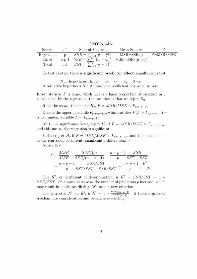
ANOVA table

Source df Sum of Squares Mean Squares FRegression p SSR =

∑ni=1(yi − y)2 MSR=SSR/p F=MSR/MSE

Error n-p-1 SSE =∑n

i=1(yi − yi)2 MSE=SSE/(n-p-1)

Total n-1 SST =∑n

i=1(yi − y)2

To test whether there is significant predictor effect, simultaneous test

Null hypothesis H0 : β1 = β2 = · · · = βp = 0 v.s.Alternative hypothesis H1: At least one coefficient not equal to zero.

If test statistic F is large, which means a large proportion of variation in yis explained by the regression, the intuition is that we reject H0.

It can be shown that under H0, F = MSR/MSE ∼ Fp,n−p−1.

Denote the upper percentile Fp,n−p−1,α, which satisfies P (F > Fp,n−p−1,α) =α for random variable F ∼ Fp,n−p−1.

At 1 − α significance level, reject H0 if F = MSR/MSE > Fp,n−p−1,α,and this means the regression is significant.

Fail to reject H0 if F = MSR/MSE < Fp,n−p−1,α, and this means noneof the regression coefficients significantly differs from 0.

Notice that

F =MSR

MSE=

SSR/(p)

SSE/(n− p− 1)=

n− p− 1

p

SSR

SST − SSR

=n− p− 1

p

SSR/SST

SST/SST − SSR/SST=

n− p− 1

p

R2

1−R2.

The R2, or coefficient of determination, is R2 = SSR/SST = 1 −SSE/SST . R2 always increase as the number of predictors p increase, whichmay result in model overfitting. We need a new criterion.

The corrected R2, or R2, is R2 = 1 − SSE/(n−p−1)SST/(n−1)

. It takes degrees offreedom into consideration and penalizes overfitting.

4

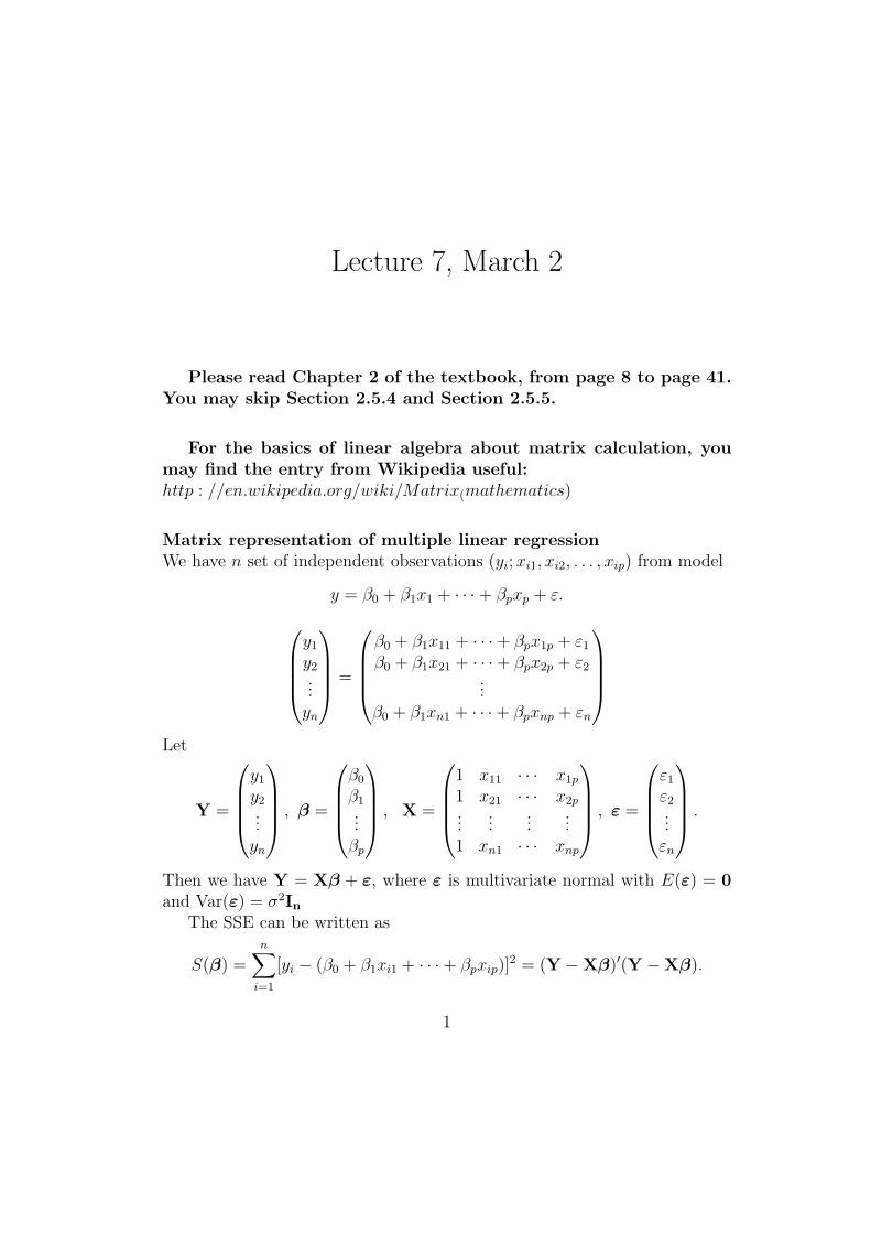
Lecture 7, March 2

Please read Chapter 2 of the textbook, from page 8 to page 41.You may skip Section 2.5.4 and Section 2.5.5.

For the basics of linear algebra about matrix calculation, youmay find the entry from Wikipedia useful:http : //en.wikipedia.org/wiki/Matrix(mathematics)

Matrix representation of multiple linear regressionWe have n set of independent observations (yi; xi1, xi2, . . . , xip) from model

y = β0 + β1x1 + · · ·+ βpxp + ε.

y1

y2...

yn

=

β0 + β1x11 + · · ·+ βpx1p + ε1

β0 + β1x21 + · · ·+ βpx2p + ε2...

β0 + β1xn1 + · · ·+ βpxnp + εn

Let

Y =

y1

y2...

yn

, β =

β0

β1...

βp

, X =

1 x11 · · · x1p

1 x21 · · · x2p...

......

...1 xn1 · · · xnp

, ε =

ε1

ε2...εn

.

Then we have Y = Xβ + ε, where ε is multivariate normal with E(ε) = 0and Var(ε) = σ2In

The SSE can be written as

S(β) =n∑

i=1

[yi − (β0 + β1xi1 + · · ·+ βpxip)]2 = (Y −Xβ)′(Y −Xβ).

1

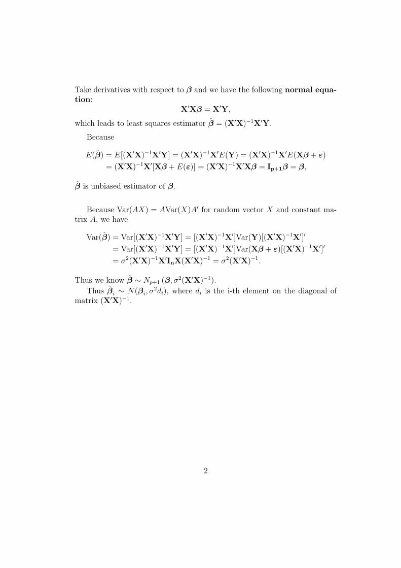
Take derivatives with respect to β and we have the following normal equa-tion:

X′Xβ = X′Y,

which leads to least squares estimator β = (X′X)−1X′Y.

Because

E(β) = E[(X′X)−1X′Y] = (X′X)−1X′E(Y) = (X′X)−1X′E(Xβ + ε)

= (X′X)−1X′[Xβ + E(ε)] = (X′X)−1X′Xβ = Ip+1β = β,

β is unbiased estimator of β.

Because Var(AX) = AVar(X)A′ for random vector X and constant ma-trix A, we have

Var(β) = Var[(X′X)−1X′Y] = [(X′X)−1X′]Var(Y)[(X′X)−1X′]′

= Var[(X′X)−1X′Y] = [(X′X)−1X′]Var(Xβ + ε)[(X′X)−1X′]′

= σ2(X′X)−1X′InX(X′X)−1 = σ2(X′X)−1.

Thus we know β ∼ Np+1 (β, σ2(X′X)−1).

Thus βi ∼ N(βi, σ2di), where di is the i-th element on the diagonal of

matrix (X′X)−1.

2