Lecture 1: Introduction to CS 5220

David Bindel

24 Aug 2011

CS 5220: Applications of Parallel Computers

http://www.cs.cornell.edu/~bindel/class/cs5220-f11/

http://www.piazza.com/cornell/cs5220

Time: TR 8:40–9:55Location: 110 HollisterInstructor: David Bindel (bindel@cs)Office: 5137 Upson HallOffice hours: M 4–5, Th 10–11, or by appt.

The Computational Science & Engineering Picture

Application

Analysis Computation

Applications Everywhere!

These tools are used in more places than you might think:I Climate modelingI CAD tools (computers, buildings, airplanes, ...)I Control systemsI Computational biologyI Computational financeI Machine learning and statistical modelsI Game physics and movie special effectsI Medical imagingI Information retrievalI ...

Parallel computing shows up in all of these.

Why Parallel Computing?

1. Scientific computing went parallel long agoI Want an answer that is right enough, fast enoughI Either of those might imply a lot of work!I ... and we like to ask for more as machines get biggerI ... and we have a lot of data, too

2. Now everyone else is going the same way!I Moore’s law continues (double density every 18 months)I But clock speeds stopped increasing around 2005

I ... otherwise we’d have power densities associated with thesun’s surface on our chips!

I But no more free speed-up with new hardware generationsI Maybe double number of cores every two years instead?I Consequence: We all become parallel programmers?

Lecture Plan

Roughly three parts:1. Basics: architecture, parallel concepts, locality and

parallelism in scientific codes2. Technology: OpenMP, MPI, CUDA/OpenCL, UPC, cloud

systems, profiling tools, computational steering3. Patterns: Monte Carlo, dense and sparse linear algebra

and PDEs, graph partitioning and load balancing, fastmultipole, fast transforms

Goals for the Class

You will learn:I Basic parallel concepts and vocabularyI Several parallel platforms (HW and SW)I Performance analysis and tuningI Some nuts-and-bolts of parallel programmingI Patterns for parallel computing in computational science

You might also learn things aboutI C and UNIX programmingI Software carpentryI Creative debugging (or swearing at broken code)

Workload

CSE usually requires teams with different backgrounds.I Most class work will be done in small groups (1–3)I Three assigned programming projects (20% each)I One final project (30%)

I Should involve some performance analysisI Best projects are attached to interesting applicationsI Final presentation in lieu of final exam

Prerequisites

You should have:I Basic familiarity with C programming

I See CS 4411: Intro to C and practice questions.I Might want Kernighan-Ritchie if you don’t have it already

I Basic numerical methodsI See CS 3220 from last semester.I Shouldn’t panic when I write an ODE or a matrix!

I Some engineering or physics is nice, but not required

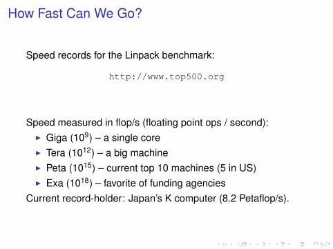
How Fast Can We Go?

Speed records for the Linpack benchmark:

http://www.top500.org

Speed measured in flop/s (floating point ops / second):I Giga (109) – a single coreI Tera (1012) – a big machineI Peta (1015) – current top 10 machines (5 in US)I Exa (1018) – favorite of funding agencies

Current record-holder: Japan’s K computer (8.2 Petaflop/s).

Peak Speed of the K Computer

(2× 109 cycles / second) ×(8 flops / cycle / core) =

16 GFlop/s / node

(16 GFlop/s / node) × (8 cores / node) =128 GFlop/s / node

(128 GFlop/s / node) ×(68544 nodes) =

8.77 GFlop/s

Linpack performance is about 93% of peak.

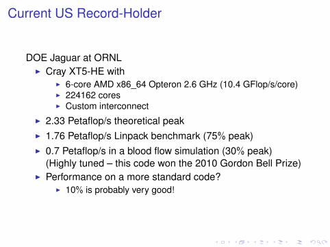
Current US Record-Holder

DOE Jaguar at ORNLI Cray XT5-HE with

I 6-core AMD x86_64 Opteron 2.6 GHz (10.4 GFlop/s/core)I 224162 coresI Custom interconnect

I 2.33 Petaflop/s theoretical peakI 1.76 Petaflop/s Linpack benchmark (75% peak)I 0.7 Petaflop/s in a blood flow simulation (30% peak)

(Highly tuned – this code won the 2010 Gordon Bell Prize)I Performance on a more standard code?

I 10% is probably very good!

Parallel Performance in Practice

So how fast can I make my computation?I Peak > Linpack > Gordon Bell > TypicalI Measuring performance of real applications is hard

I Typically a few bottlenecks slow things downI And figuring out why they slow down can be tricky!

I And we really care about time-to-solutionI Sophisticated methods get answer in fewer flopsI ... but may look bad in benchmarks (lower flop rates!)

See also David Bailey’s comments:I Twelve Ways to Fool the Masses When Giving Performance

Results on Parallel Computers (1991)I Twelve Ways to Fool the Masses: Fast Forward to 2011 (2011)

Quantifying Parallel Performance

I Starting point: good serial performanceI Strong scaling: compare parallel to serial time on the same

problem instance as a function of number of processors (p)

Speedup =Serial time

Parallel time

Efficiency =Speedup

p

I Ideally, speedup = p. Usually, speedup < p.I Barriers to perfect speedup

I Serial work (Amdahl’s law)I Parallel overheads (communication, synchronization)

Amdahl’s Law

Parallel scaling study where some serial code remains:

p = number of processorss = fraction of work that is serialts = serial timetp = parallel time ≥ sts + (1− s)ts/p

Amdahl’s law:

Speedup =tstp

=1

s + (1− s)/p>

1s

So 1% serial work =⇒ max speedup < 100×, regardless of p.

A Little Experiment

Let’s try a simple parallel attendance count:I Parallel computation: Rightmost person in each row

counts number in row.I Synchronization: Raise your hand when you have a countI Communication: When all hands are raised, each row

representative adds their count to a tally and says the sum(going front to back).

(Somebody please time this.)

A Toy Analysis

Parameters:

n = number of studentsr = number of rows

tc = time to count one studenttt = time to say tallyts ≈ ntctp ≈ ntc/r + rtt

How much could I possibly speed up?

Modeling Speedup

0 2 4 6 8 10 120.6

0.8

1

1.2

1.4

Rows

Pre

dict

edsp

eedu

p

(Parameters: n = 55, tc = 0.3, tt = 2.)

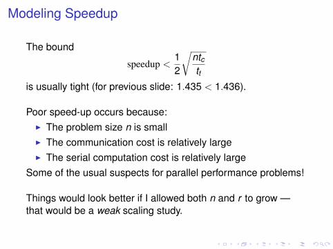
Modeling Speedup

The bound

speedup <12

√ntctt

is usually tight (for previous slide: 1.435 < 1.436).

Poor speed-up occurs because:I The problem size n is smallI The communication cost is relatively largeI The serial computation cost is relatively large

Some of the usual suspects for parallel performance problems!

Things would look better if I allowed both n and r to grow —that would be a weak scaling study.

Summary: Thinking about Parallel Performance

Today:I We’re approaching machines with peak exaflop ratesI But codes rarely get peak performanceI Better comparison: tuned serial performanceI Common measures: speedup and efficiencyI Strong scaling: study speedup with increasing pI Weak scaling: increase both p and nI Serial overheads and communication costs kill speedupI Simple analytical models help us understand scaling

Next time: Computer architecture and serial performance.

And in case you arrived late

http://www.cs.cornell.edu/~bindel/class/cs5220-f11/

http://www.piazza.com/cornell/cs5220