Lect 8

PolyE-501

ADVANCED POLYMER RHEOLOGY

Dr. M. Shafiq IrfanAssistant Professor

Department of Polymer and Process Engineering

University of Engineering and Technology, Lahore

PRINCIPLES OF LINEARVISCOELASTICITY*

2* I M Ward and J Sweeney, The Mechanical Properties of Solid Polymers: Chapter 4

hp

Highlight

Viscoelasticity as a phenomenon

3

Viscoelasticity as a Phenomenon

• The behaviour of materials of low relative molecular mass is usually discussed in terms of two particular types of ideal material: the elastic solid and the viscous liquid.

• One of the most interesting features of polymers is that a given polymer can display all the intermediate range of properties between an elastic solid and a viscous liquid depending on the temperature and the experimentally chosen timescale. This form of response is termed viscoelasticity.

4

Linear Viscoelastic Behaviour

Hooke’s law describes the behaviour of a linear elastic solid and Newton’s law that of a linear viscous liquid. A simple constitutive relation for the behaviour of a linear viscoelastic solid is obtained by combining these two laws:

1. For elastic behaviour

2. For viscous behaviour

5


• A simple possible formulation of linear viscoelastic behaviour combines these equations, making the assumption that the shear stresses related to strain and strain rate are additive:

• The equation represents one of the simple models for linear viscoelastic behaviour, the Kelvin or Voigt model.

6


• For elastic solids Hooke’s law is valid only at small strains, and Newton’s law of viscosity is restricted to relatively low flow rates, as only when the stress is proportional either to the strain or the strain rate is analysis of the deformation feasible in simple form.

• A comparable limitation holds for viscoelastic materials: general quantitative predictions are possible only in the case of linear viscoelasticity, for which the results of changing stresses or strains are simply additive, but the time at which the change is made must be taken into account.

7

Creep

• Creep is the time-dependent change in strain following a step change in stress.

• The responses to two levels of stress for linear elastic and linear viscoelastic materials are compared in Figure 4.2.

• In the former case the strain follows the pattern of the loading programme exactly and in exact proportionality to the magnitude of the stresses applied.

8

9

Creep

• For the most general case of a linear viscoelastic solid the total strain e is the sum of three essentially separate parts:

• e1 the immediate elastic deformation

• e2 the delayed elastic deformation

• e3 the Newtonian flow, which is identical with the deformation of a viscous liquid obeying Newton’s law of viscosity.

10

Creep

• Because the material shows linear behaviour the magnitudes of e1, e2 and e3 are exactly proportional to the magnitude of the applied stress, so that a creep compliance J(t) can be defined, which is a function of time only:

where J1, J2 and J3 correspond to e1, e2 and e3.

11

Creep

• Linear amorphous polymers show a significant J3

above their glass transition temperatures, when creep may continue until the specimen ruptures, but at lower temperatures J1 and J2 dominate.

• Crosslinked polymers do not show a J3 term, and to a very good approximation neither do highly crystalline polymers.

• The maximum insight into the nature of creep is obtained by plotting the logarithm of creep compliance against the logarithm of time over a very wide time-scale (Figure 4.3).

12

Creep

13

Creep

• It is convenient to define a retardation time τ’ in the middle of the viscoelastic region to characterize the time-scale for creep. The distinction between a rubber and a glassy plastic is then seen to be somewhat artificial, because it depends only on the value of τ’ at room temperature.

• Compared with typical experimental response times, which can rarely be less than 1 s, τ’ for a rubber is very small at room temperature, whereas the opposite is true for a glassy polymer.

14

Creep

• As the temperature is raised the frequency of molecular rearrangements increases, so reducing the value of τ’ .

• Thus at sufficiently low temperatures a rubber behaves like a glassy plastic, and will shatter under impact conditions; correspondingly a glassy plastic will become rubber-like at a sufficiently high temperature.

15

Stress Relaxation

• When an instantaneous strain is applied to an ideal elastic solid a finite and constant stress will be recorded. For a linear viscoelastic solid subjected to a nominally instantaneous strain the initial stress will be proportional to the applied strain and will decrease with time (Figure 4.4), at a rate characterized by the relaxation time τ. This behaviour is called stress relaxation.

• For amorphous linear polymers at high temperatures the stress may eventually decay to zero.

16

Stress Relaxation

17

Stress Relaxation

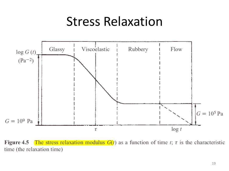
• Making the assumption of linear viscoelastic behaviour we can define the stress relaxation modulus G(t) = σ(t)/e. Where there is no viscous flow the stress decays to a finite value (Figure 4.5), to give an equilibrium or relaxed modulus Gr

at finite time.

• As with creep we see that there are regions of glassy, viscoelastic, rubberlike and flow behaviour; similarly, changing temperature is equivalent to changing the time-scale.

18

Stress Relaxation

19

Mathematical representation of linear viscoelasticity

20

The Boltzmann superposition principle

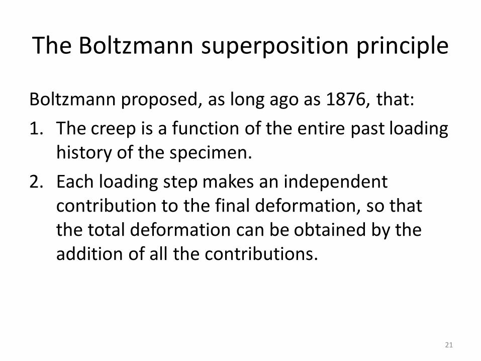
Boltzmann proposed, as long ago as 1876, that:

1. The creep is a function of the entire past loading history of the specimen.

2. Each loading step makes an independent contribution to the final deformation, so that the total deformation can be obtained by the addition of all the contributions.

21


22


• The total creep at time t is then given by

where J(t - τ) is the creep compliance function.

• The summation of above Equation can be generalized in integral form as

• Separating out the instantaneous elastic response in terms of the unrelaxed modulus Gu gives

23


• The integral in last Equation is called a Duhamel integral, and it is a useful illustration of the consequences of the Boltzmann superposition principle to evaluate the response for a number of simple loading programmes.

• The Duhamel integral is most simply evaluated by treating it as the summation of a number of response terms.

24

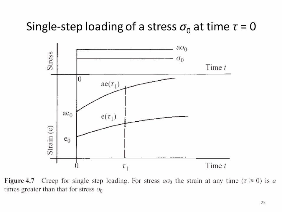
Single-step loading of a stress σ0 at time τ = 0

25

Two-step loading of a stress σ0 at time τ = 0 , followed by an additional stress σ0 at time τ = t1

26

Creep and Recovery

27

Mechanical models, retardation and relaxation time spectra

28

Mechanical Models

29

Mechanical Models

• We have seen that the Maxwell model describes the stress relaxation of a viscoelastic solid to a first approximation, and the Kelvin model the creep behaviour, but that neither model is adequate for the general behaviourof a viscoelastic solid where it is necessary to describe both stress relaxation and creep.

30

The Standard Linear Solid

• A response closer to that of a real polymer is obtained by adding a second spring of modulus Ea in parallel with a Maxwell unit (Figure 4.12). This model is known as the ‘standard linear solid’ and is usually attributed to Zener.

• It provides an approximate representation to the observed behaviour of polymers in their viscoelastic range.

31


32


• In creep, both springs extend, so that

but in stress relaxation Ea is unaffected, giving

• The stress–strain relationship is

33

Multi-element models

• For real materials a simple exponential response in creep or stress relaxation is not an adequate description of the time dependence.

• A good representation can be obtained by simulating creep with an array of Kelvin models in series and simulating stress relaxation with an array of Maxwell models in parallel (Figure 4.13).

34


35


36

Retardation and relaxation time spectra

• Let the number of individual units in multi-element models tend to infinity. For creep, an infinite number of Kelvin units gives an infinite number of retardation times: this is called the spectrum of retardation times.

• The analagous development for stress relaxation leads to the spectrum of relaxation times.

37

Documents

Lect 8