lec06_P

Curves and Splines

Outline

• Hermite Splines

• Catmull-Rom Splines

• Bezier Curves

• Higher Continuity: Natural and B-Splines

• Drawing Splines

3

Modeling Complex Shapes

• We want to build models of very complicated objects

• An equation for a sphere is possible, but how about an equation for a telephone, or a face?

• Complexity is achievedusing simple pieces

– polygons, parametric curvesand surfaces, or implicit

curves and surfaces

– This lecture: parametriccurves

4

What Do We Need From Curvesin Computer Graphics?

• Local control of shape (so that easy to build and modify)

• Stability

• Smoothness and continuity

• Ability to evaluate derivatives

• Ease of rendering

Demo

Curve Usage Demo

5

Curve Representations

• Explicit: y = f(x)

– Easy to generate points

– Must be a function: big limitation—vertical lines?

bmxy +=

x

y

6



– Easy to generate points


bmxy +=

x

y

•Implicit: f(x,y) = 0

+Easy to test if on the curve

–Hard to generate points

0222=!+ ryx

x

y

7



+ Easy to generate points


bmxy +=

x

y

•Implicit: f(x,y) = 0

+Easy to test if on the curve

–Hard to generate points

0222=!+ ryx

x

y

•Parametric: (x,y) = ( f(u), g(u))

+Easy to generate points

)sin,(cos),( uuyx =

u=0

u=""""/2

u= """"

8

Parameterization of a Curve

• Parameterization of a curve: how a change in u moves you along a given curve in xyz space.

• There are an infinite number of parameterizations of a given curve. Slow, fast, speed continuous or discontinuous, clockwise (CW) or CCW…

9

Polynomial Interpolation

• An n-th degree polynomial fits a curve to n+1 points

– called Lagrange Interpolation

– result is a curve that is too wiggly, change to any control point affects entire curve (nonlocal) – this method is poor

• We usually want the curve to be as smooth as possible

– minimize the wiggles

– high-degree polynomials are bad

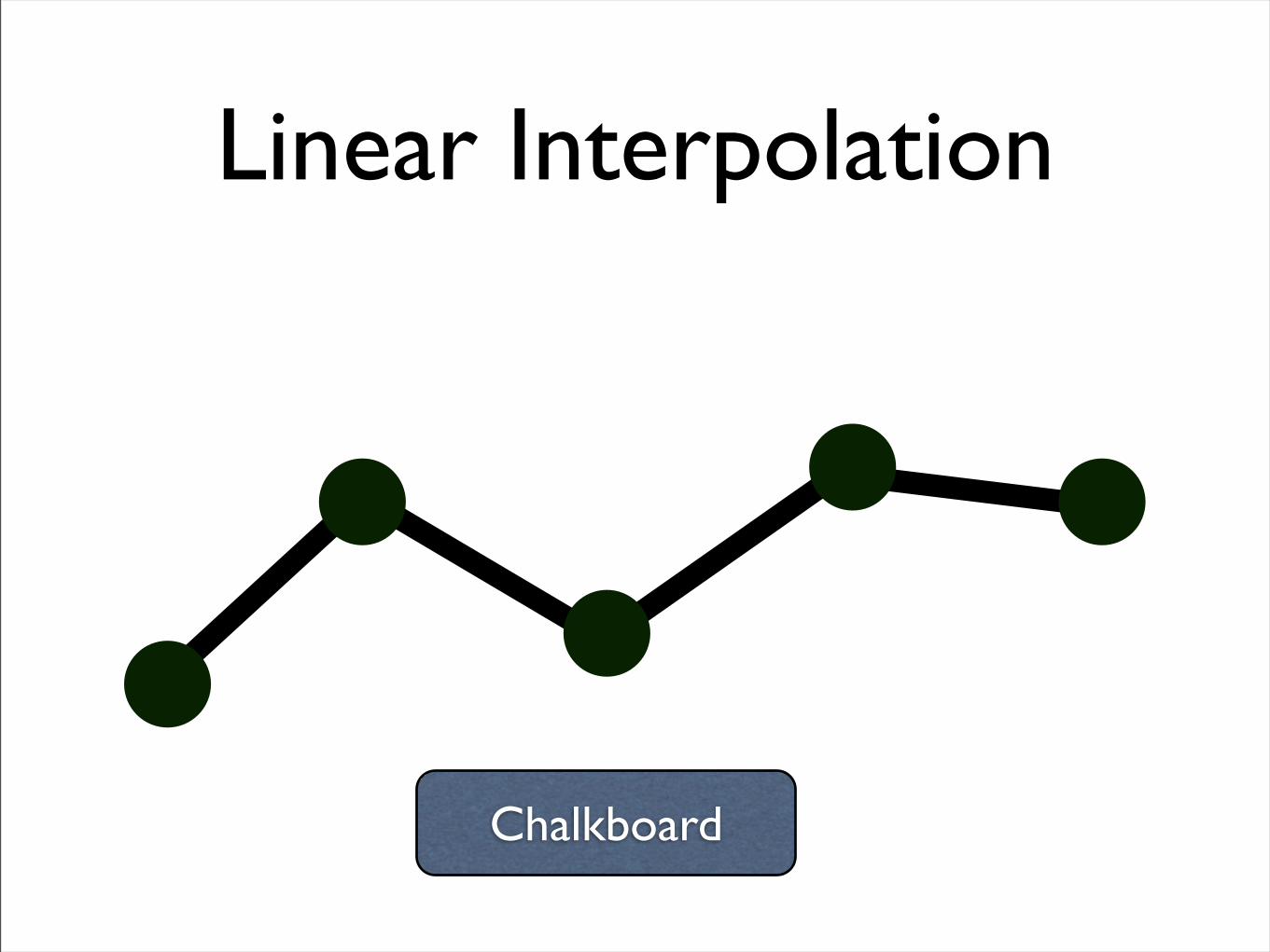
Linear Interpolation

Chalkboard

Spline Interpolation

Spine Interpolation Demo

10

Splines: Piecewise Polynomials

• A spline is a piecewise polynomial - many low degree

polynomials are used to interpolate (pass through) the

control points

• Cubic piecewise polynomials are the most common:

– piecewise definition gives local control

11

Piecewise Polynomials

• Spline: lots of little polynomials pieced together

• Want to make sure they fit together nicely

Continuous in position

Continuous in position and tangent vector

Continuous in position, tangent, and curvature

12

Splines

• Types of splines:– Hermite Splines

– Catmull-Rom Splines

– Bezier Splines

– Natural Cubic Splines

– B-Splines

– NURBS

7

Hermite Curves

• Cubic Hermite Splines

That is, we want a way to specify the end points and theslope at the end points!

Po

P1

P2

13

Splines

chalkboard

14

The Cubic Hermite Spline Equation

control matrix(what the user gets to pick)

basispoint thatgets drawn

• Using some algebra, we obtain:

[ ]!!!!

"

#

$$$$

%

&

!

!!!!!

"

#

$$$$

%

&

"""

"

=

2

1

2

1

23

0001

0100

1233

1122

1)(

p

p

p

p

uuuup

• This form typical for splines– basis matrix and meaning of control matrix change with

the spline type

15

The Cubic Hermite Spline Equation

control matrix(what the user gets to pick)

basispoint thatgets drawn

• Using some algebra, we obtain:

[ ]!!!!

"

#

$$$$

%

&

!

!!!!!

"

#

$$$$

%

&

"""

"

=

2

1

2

1

23

0001

0100

1233

1122

1)(

p

p

p

p

uuuup

!!!!

"

#

$$$$

%

&

!

!

!!!!!

"

#

$$$$$

%

&

"

+"

+"

+"

=

2

1

2

1

23

23

23

23

2

32

132

)(

p

p

p

p

uu

uuu

uu

uu

up4 Basis Functions

T

16

Every cubic Hermite spline is a linear combination (blend)of these 4 functions

!!!!

"

#

$$$$

%

&

!

!

!!!!!

"

#

$$$$$

%

&

"

+"

+"

+"

=

2

1

2

1

23

23

23

23

2

32

132

)(

p

p

p

p

uu

uuu

uu

uu

up

4 Basis Functions

Four Basis Functions for Hermite splines

T

u

17

Piecing together Hermite Curves

• It's easy to make a multi-segment Hermite spline

– each piece is specified by a cubic Hermite curve

– just specify the position and tangent at each “joint”

– the pieces fit together with matched positions and first derivatives

– gives C1 continuity

• The points that the curve has to pass through are called knots or knot points

Outline

• Hermite Splines


• Bezier Curves


• Drawing Splines

Problem with Hermite Splines?

• Must explicitly specify derivatives at each endpoint!

• How can we solve this?

8

Catmull-Rom Splines

• Use for the roller-coaster assignment

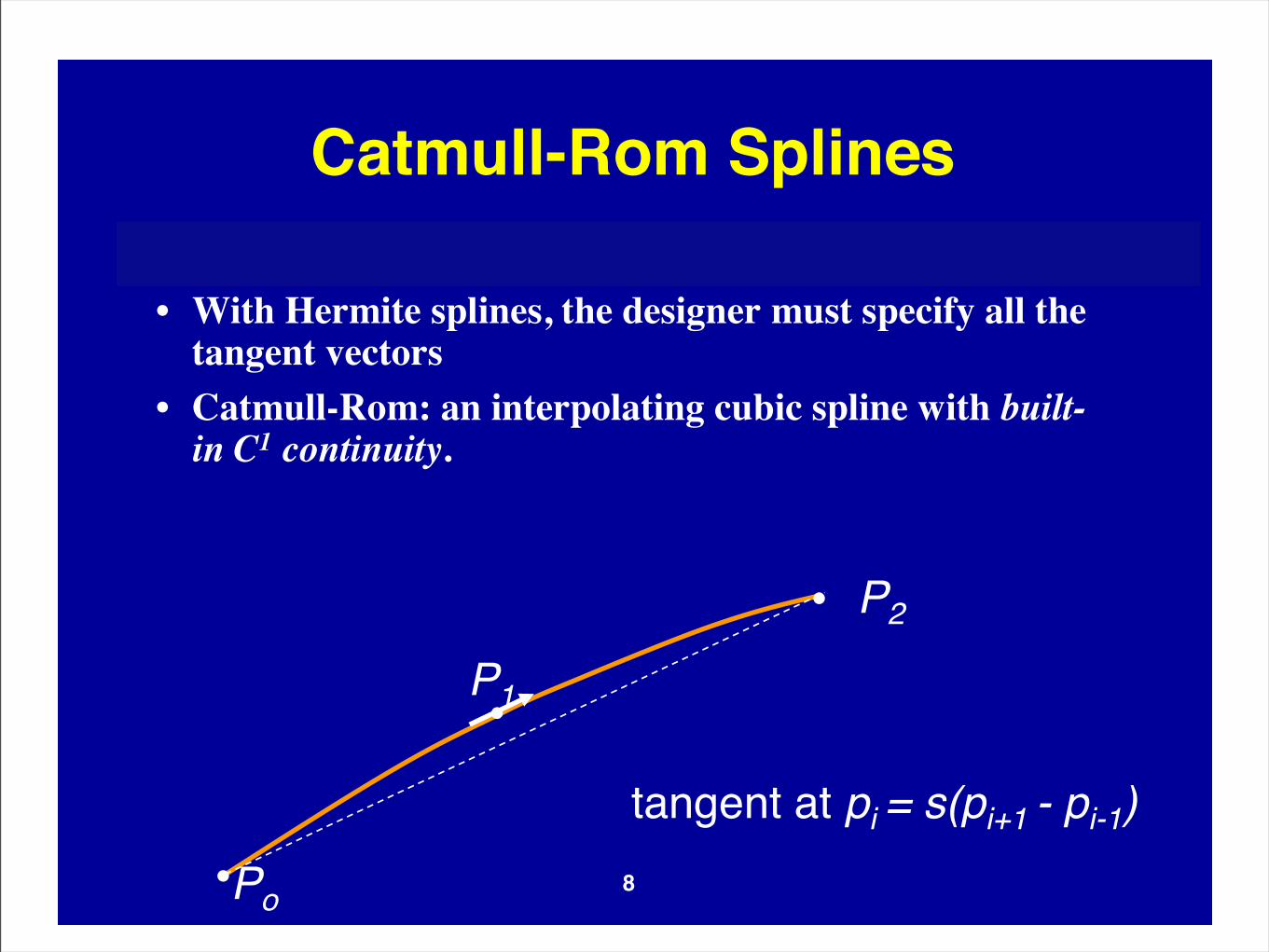
• With Hermite splines, the designer must specify all the tangent vectors

• Catmull-Rom: an interpolating cubic spline with built-in C1 continuity.

Po

P1

P2

tangent at pi = s(pi+1 - pi-1)

18

Catmull-Rom Splines

• Use for the roller-coaster (next programming assignment)

• With Hermite splines, the designer must arrange for consecutive tangents to be collinear, to get C1

continuity. This gets tedious.


chalkboard

19

Catmull-Rom Spline Matrix

control vectorCR basisspline coefficients

[ ]!!!!

"

#

$$$$

%

&

!!!!

"

#

$$$$

%

&

!

!!!

!!!

=

4

3

2

1

23

0010

00

2332

22

1)(

p

p

p

p

ss

ssss

ssss

uuuup

• Derived similarly to Hermite

• Parameter s is typically set to s=1/2.

20


[ ] [ ]!!!!

"

#

$$$$

%

&

!!!!

"

#

$$$$

%

&

!

!!!

!!!

=

444

333

222

111

23

0010

00

2332

22

1

zyx

zyx

zyx

zyx

ss

ssss

ssss

uuuzyx

control vectorCR basisspline coefficients

9

Catmull-Rom Splines

• Use for the roller-coaster assignment

• With Hermite splines, the designer must specify all the tangent vectors


10


control vectorCR basis

[ ]!!!!

"

#

$$$$

%

&

!!!!

"

#

$$$$

%

&

!

!!!

!!!

=

4

3

2

1

23

0010

00

2332

22

1)(

p

p

p

p

ss

ssss

ssss

uuuup

• Derived similarly to Hermite

• Parameter s is typically set to s=1/2.

11

Cubic Curves in 3D

• Three cubic polynomials, one for each coordinate

– x(u) = axu3+bxu

2+cxu+dx

– y(u) = ayu3+byu

2+cyu+dy

– z(u) = azu3+bzu

2+czu+dz

• In matrix notation

[ ] [ ]!!!!

"

#

$$$$

%

&

=

zyx

zyx

zyx

zyx

ddd

ccc

bbb

aaa

uuuuzuyux 1)()()(23

12

Catmull-Rom Spline Matrix in 3D

[ ] [ ]!!!!

"

#

$$$$

%

&

!!!!

"

#

$$$$

%

&

!

!!!

!!!

=

444

333

222

111

23

0010

00

2332

22

1)()()(

zyx

zyx

zyx

zyx

ss

ssss

ssss

uuuuzuyux


Outline

• Hermite Splines


• Bezier Curves


• Drawing Splines

Problem withCatmull-Rom Splines?

• No control of derivatives at endpoints!

• How can we solve this?

• We want something intuitive.

13

Bezier Curves*

• Another variant of the same game

• Instead of endpoints and tangents, four control points

– points P0 and P3 are on the curve: P(u=0) = P0, P(u=1) = P3

– points P1 and P2 are off the curve

– P'(u=0) = 3(P1-P0), P'(u=1) = 3(P3 – P2)

• Convex Hull property

– curve contained within convex hull of control points

• Gives more control knobs (series of points) than Hermite

• Scale factor (3) is chosen to make “velocity” approximately constant

Bezier Spline Example

14

The Bezier Spline Matrix*

[ ] [ ]!!!!

"

#

$$$$

%

&

!!!!

"

#

$$$$

%

&

!

!

!!

=

444

333

222

111

23

0001

0033

0363

1331

1

zyx

zyx

zyx

zyx

uuuzyx

Bezier basis Bezier

control vector

15

Bezier Blending Functions*

Also known as the order 4, degree 3 Bernstein polynomials

Nonnegative, sum to 1

The entire curve lies inside the polyhedron bounded by the control points

Outline

• Hermite Splines


• Bezier Curves


• Drawing Splines

16

Piecewise Polynomials

• Spline: lots of little polynomials pieced together

• Want to make sure they fit together nicely

Continuous in position

Continuous in position and tangent vector

Continuous in position, tangent, and curvature

17

Splines with More Continuity?

• How could we get C2 continuity at control points?

• Possible answers:

– Use higher degree polynomials

degree 4 = quartic, degree 5 = quintic, … but these get computationally expensive, and sometimes wiggly

– Give up local control natural cubic splines

A change to any control point affects the entire curve

– Give up interpolation cubic B-splines

Curve goes near, but not through, the control points

18

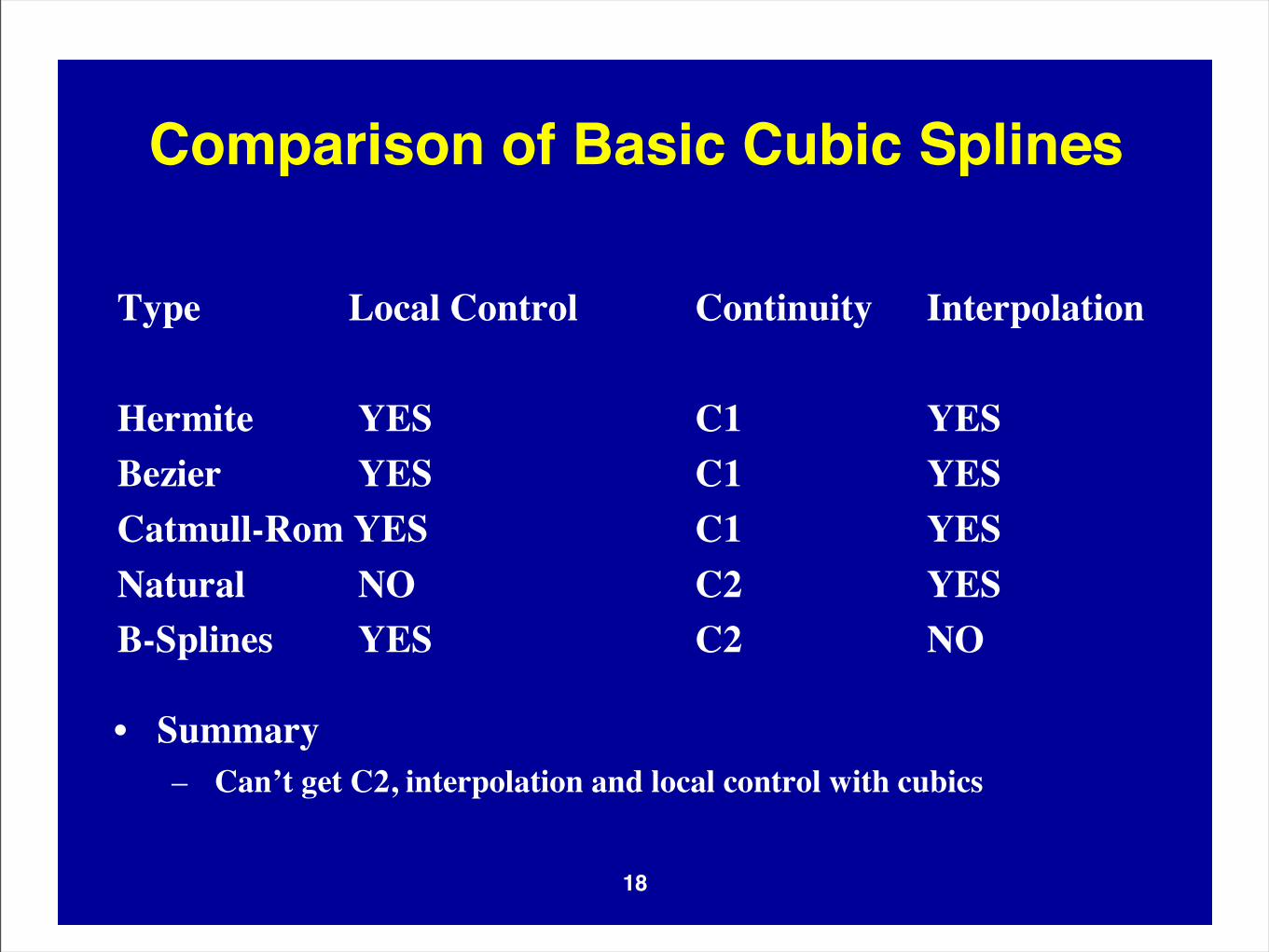
Comparison of Basic Cubic Splines

Type Local Control Continuity Interpolation

Hermite YES C1 YES

Bezier YES C1 YES

Catmull-Rom YES C1 YES

Natural NO C2 YES

B-Splines YES C2 NO

• Summary

– Can’t get C2, interpolation and local control with cubics

19

Natural Cubic Splines*

• If you want 2nd derivatives at joints to match up, the resulting curves are called natural cubic splines

• It’s a simple computation to solve for the cubics' coefficients. (See Numerical Recipes in C book for code.)

• Finding all the right weights is a global calculation (solve tridiagonal linear system)

20

B-Splines*

• Give up interpolation

– the curve passes near the control points

– best generated with interactive placement (because it’s hard to guess where the curve will go)

• Curve obeys the convex hull property

• C2 continuity and local control are good compensation for loss of interpolation

21

B-Spline Basis*

• We always need 3 more control points than splinepieces

!!!!

"

#

$$$$

%

&

=

!!!!

"

#

$$$$

%

&

!

!

!!

=

!

!

!

i

i

i

i

Bs

Bs

P

P

P

P

G

M

i

1

2

3

0141

0303

0363

1331

6

1

Outline

• Hermite Splines


• Bezier Curves


• Drawing Splines

22

How to Draw Spline Curves

• Basis matrix eqn. allows same code to draw any spline type

• Method 1: brute force

– Calculate the coefficients

– For each cubic segment, vary u from 0 to 1 (fixed step size)

– Plug in u value, matrix multiply to compute position on curve

– Draw line segment from last position to current position

[ ] [ ]!!!!

"

#

$$$$

%

&

!!!!

"

#

$$$$

%

&

!

!!!

!!!

=

444

333

222

111

23

0010

00

2332

22

1

zyx

zyx

zyx

zyx

ss

ssss

ssss

uuuzyx


23

How to Draw Spline Curves• What’s wrong with this approach?

–Draws in even steps of u

–Even steps of u !!!! even steps of x

–Line length will vary over the curve

–Want to bound line length

»too long: curve looks jagged

»too short: curve is slow to draw

24

Drawing Splines, 2

• Method 2: recursive subdivision - vary step size to draw short lines

Subdivide(u0,u1,maxlinelength)umid = (u0 + u1)/2x0 = P(u0)x1 = P(u1)if |x1 - x0| > maxlinelength

Subdivide(u0,umid,maxlinelength)Subdivide(umid,u1,maxlinelength)

else drawline(x0,x1)

• Variant on Method 2 - subdivide based on curvature

– replace condition in “if” statement with straightness criterion

– draws fewer lines in flatter regions of the curve

25

In Summary...• Summary:

– piecewise cubic is generally sufficient

– define conditions on the curves and their continuity

• Things to know:

– basic curve properties (what are the conditions, controls, and properties for each spline type)

– generic matrix formula for uniform cubic splines x(u) = uBG

– given definition derive a basis matrix

Documents

lec06_P