Lec Diffvcvvbv

Module5/Lesson3

1 Applied Elasticity for Engineers T.G.Sitharam & L.GovindaRaju

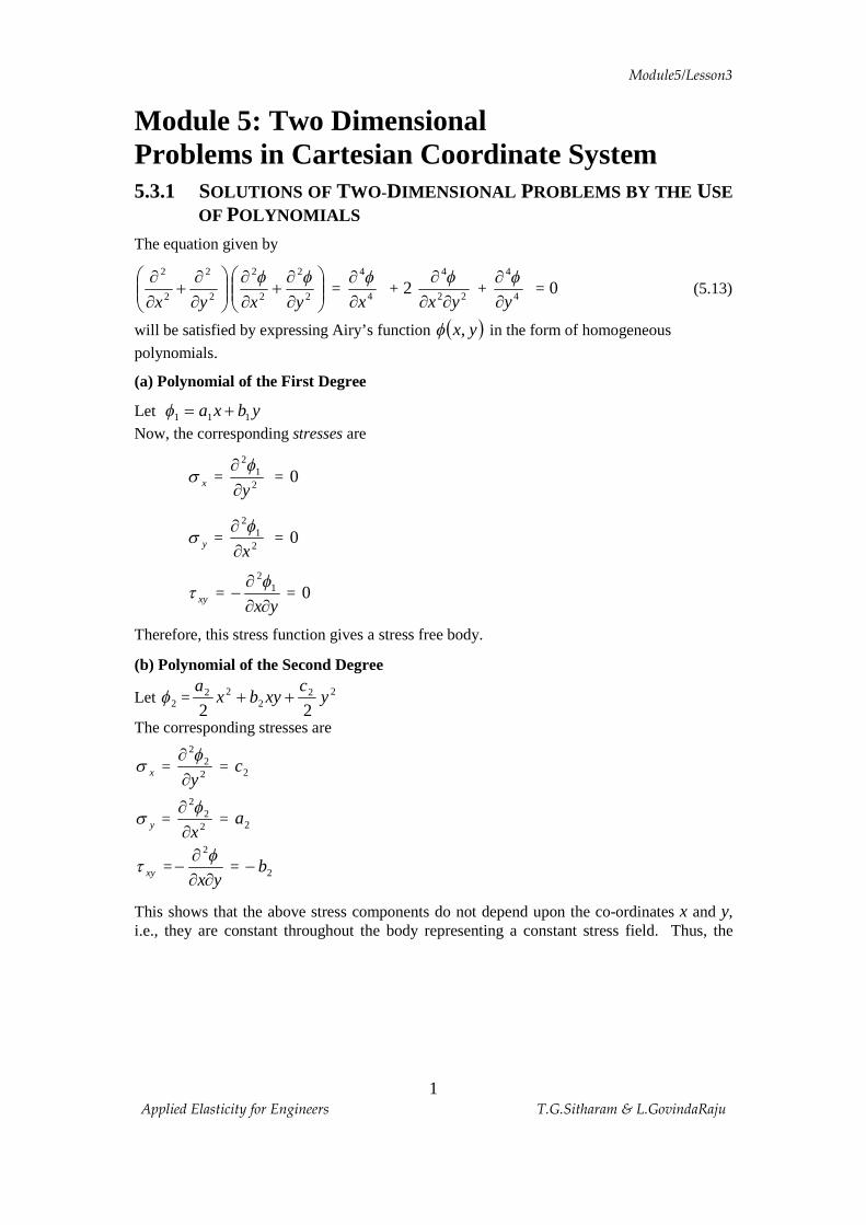
Module 5: Two Dimensional Problems in Cartesian Coordinate System 5.3.1 SOLUTIONS OF TWO-DIMENSIONAL PROBLEMS BY THE USE

OF POLYNOMIALS

The equation given by

÷÷ø

öççè

æ¶¶

+¶¶

2

2

2

2

yx ÷÷ø

öççè

æ¶¶

+¶¶

2

2

2

2

yx

ff =

4

4

x¶¶ f

+ 2 22

4

yx ¶¶¶ f

+ 4

4

y¶¶ f

= 0 (5.13)

will be satisfied by expressing Airy’s function ( )yx,f in the form of homogeneous polynomials.

(a) Polynomial of the First Degree

Let ybxa 111 +=f Now, the corresponding stresses are

xs = 21

2

y¶¶ f

= 0

ys = 21

2

x¶¶ f

= 0

xyt = yx¶¶

¶- 1

2f = 0

Therefore, this stress function gives a stress free body.

(b) Polynomial of the Second Degree

Let 2f = 222

22

22y

cxybx

a++

The corresponding stresses are

xs = 22

2

y¶¶ f

= 2c

ys = 22

2

x¶¶ f

= 2a

xyt =yx¶¶

¶-

f2

= 2b-

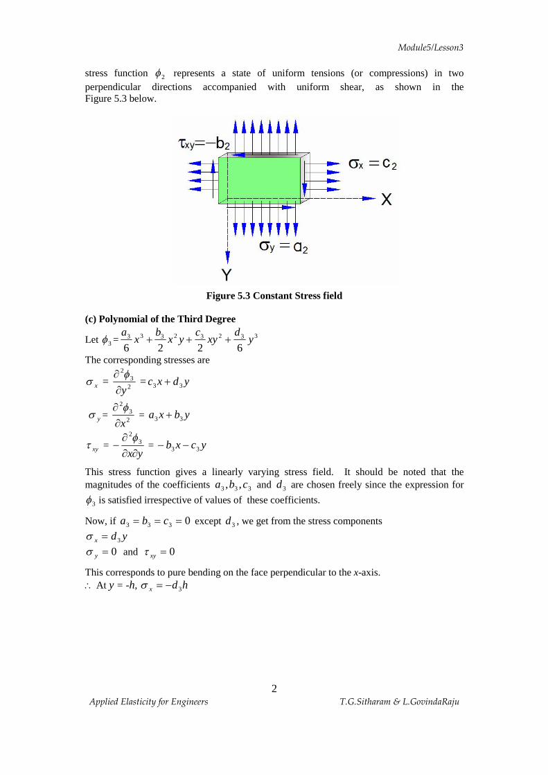
This shows that the above stress components do not depend upon the co-ordinates x and y, i.e., they are constant throughout the body representing a constant stress field. Thus, the

Module5/Lesson3


stress function 2f represents a state of uniform tensions (or compressions) in two perpendicular directions accompanied with uniform shear, as shown in the Figure 5.3 below.

Figure 5.3 State of stresses

Figure 5.3 Constant Stress field (c) Polynomial of the Third Degree

Let 3f = 33232333

6226y

dxy

cyx

bx

a+++

The corresponding stresses are

xs = 23

2

y¶¶ f

= ydxc 33 +

ys = 23

2

x¶¶ f

= ybxa 33 +

xyt = yx¶¶

¶- 3

2f = ycxb 33 --

This stress function gives a linearly varying stress field. It should be noted that the magnitudes of the coefficients 333 ,, cba and 3d are chosen freely since the expression for

3f is satisfied irrespective of values of these coefficients.

Now, if 0333 === cba except 3d , we get from the stress components

ydx 3=s

0=ys and 0=xyt

This corresponds to pure bending on the face perpendicular to the x-axis. \ At y = -h, hdx 3-=s

Module5/Lesson3


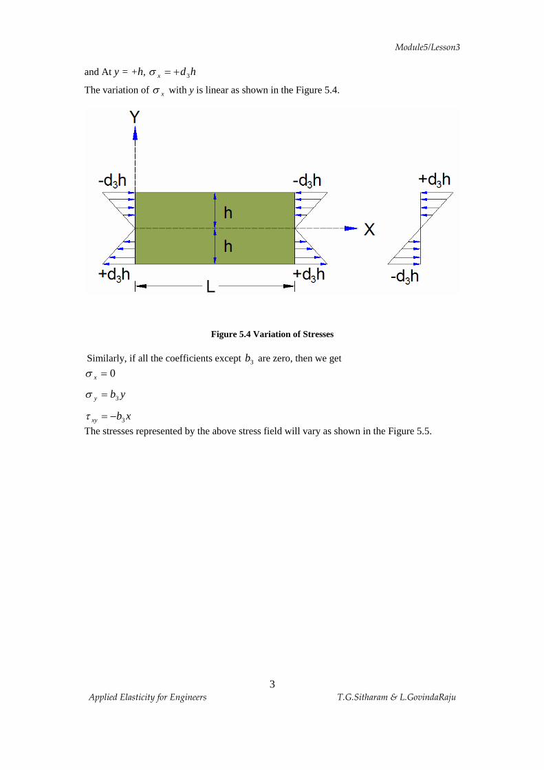
and At y = +h, hdx 3+=s

The variation of xs with y is linear as shown in the Figure 5.4.

Figure 5.4 Variation of Stresses

Similarly, if all the coefficients except 3b are zero, then we get

0=xs

yby 3=s

xbxy 3-=t

The stresses represented by the above stress field will vary as shown in the Figure 5.5.

Module5/Lesson3


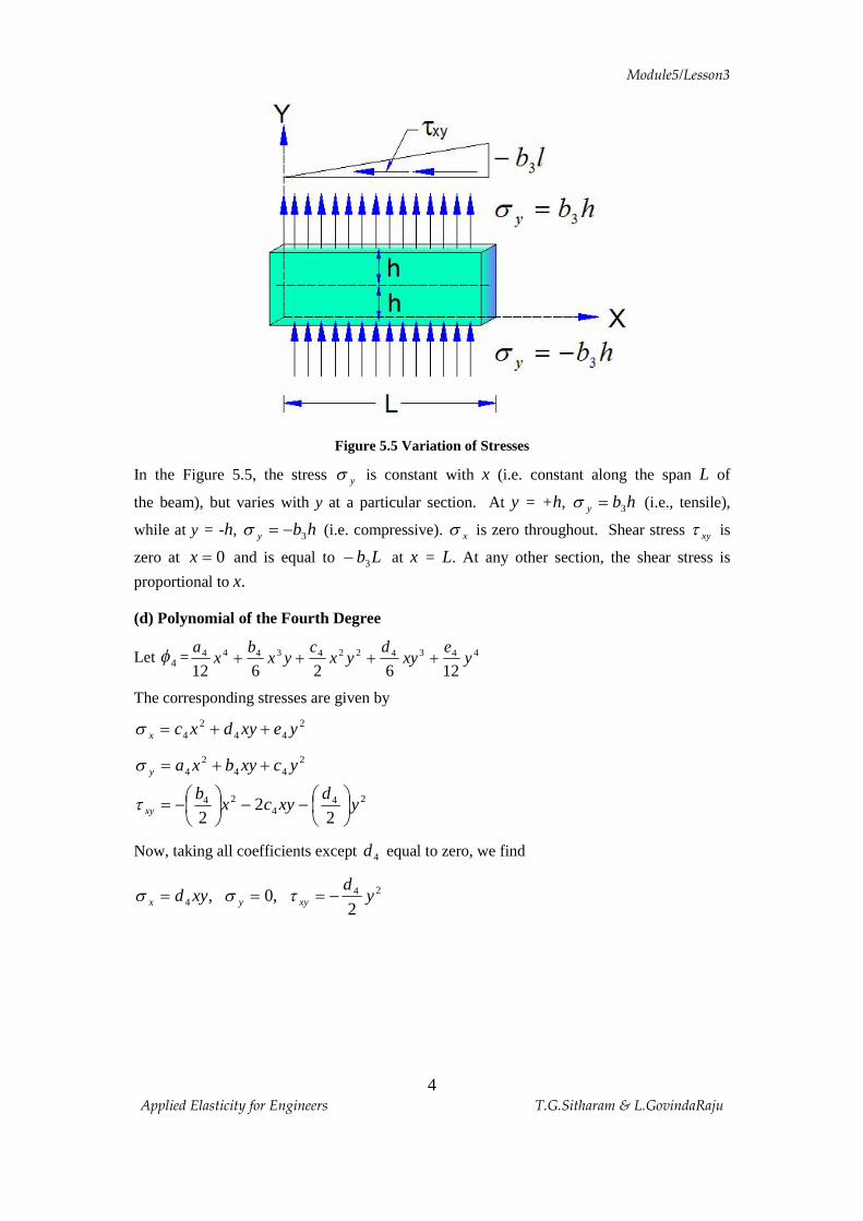
Figure 5.5 Variation of Stresses

In the Figure 5.5, the stress ys is constant with x (i.e. constant along the span L of

the beam), but varies with y at a particular section. At y = +h, hby 3=s (i.e., tensile),

while at y = -h, hby 3-=s (i.e. compressive). xs is zero throughout. Shear stress xyt is

zero at 0=x and is equal to Lb3- at x = L. At any other section, the shear stress is

proportional to x.

(d) Polynomial of the Fourth Degree

Let 4f = 44342243444

1262612y

exy

dyx

cyx

bx

a++++

The corresponding stresses are given by

244

24 yexydxcx ++=s

244

24 ycxybxay ++=s

244

24

22

2y

dxycx

bxy ÷

øö

çèæ--÷

øö

çèæ-=t

Now, taking all coefficients except 4d equal to zero, we find

,4 xydx =s ,0=ys 24

2y

dxy -=t

Module5/Lesson3


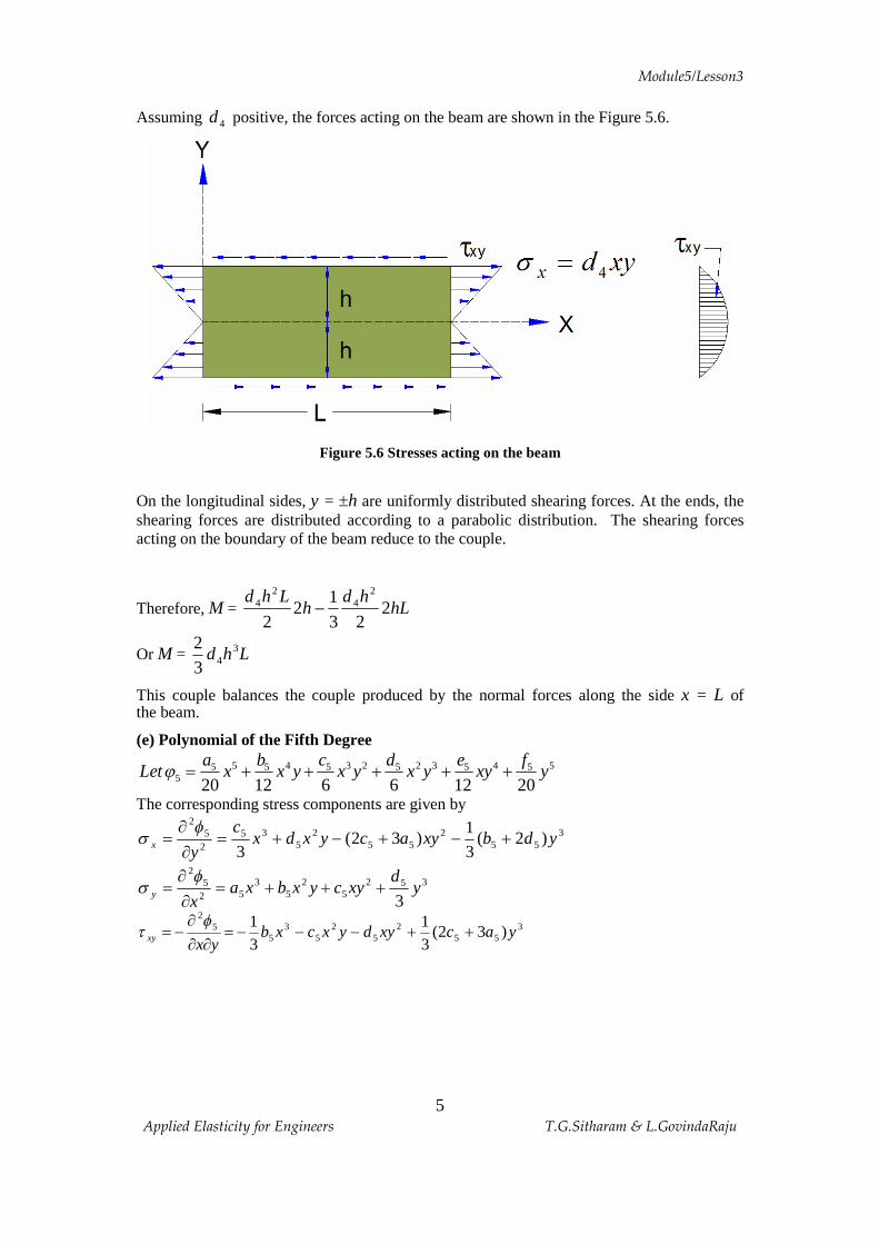
Assuming 4d positive, the forces acting on the beam are shown in the Figure 5.6.

Figure 5.6 Stresses acting on the beam

On the longitudinal sides, y = ±h are uniformly distributed shearing forces. At the ends, the shearing forces are distributed according to a parabolic distribution. The shearing forces acting on the boundary of the beam reduce to the couple.

Therefore, M = hLhd

hLhd

223

12

2

24

24 -

Or M = Lhd 343

2

This couple balances the couple produced by the normal forces along the side x = L of the beam.

(e) Polynomial of the Fifth Degree

5 4 3 2 2 3 4 55 5 5 5 5 55 20 12 6 6 12 20

a b c d e fLet x x y x y x y xy yj = + + + + +

The corresponding stress components are given by

355

255

25

3525

2

)2(31

)32(3

ydbxyacyxdxc

yx +-+-+=¶¶

=f

s

3525

25

352

52

3y

dxycyxbxa

xy +++=¶¶

=f

s

355

25

25

35

52

)32(31

31

yacxydyxcxbyxxy ++---=

¶¶¶

-=f

t

Module5/Lesson3


Here the coefficients 5555 ,,, dcba are arbitrary, and in adjusting them we obtain solutions

for various loading conditions of the beam.

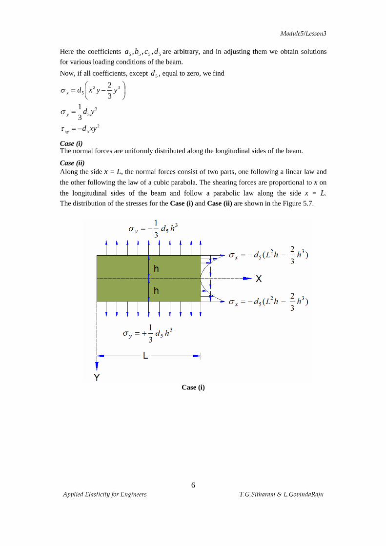
Now, if all coefficients, except 5d , equal to zero, we find

÷øö

çèæ -= 32

5 32

yyxdxs

25

353

1

xyd

yd

xy

y

-=

=

t

s

Case (i) The normal forces are uniformly distributed along the longitudinal sides of the beam.

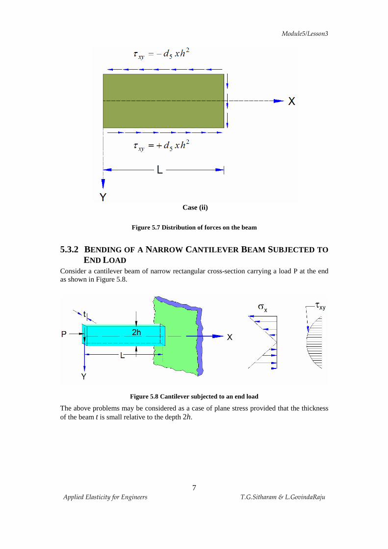
Case (ii) Along the side x = L, the normal forces consist of two parts, one following a linear law and

the other following the law of a cubic parabola. The shearing forces are proportional to x on

the longitudinal sides of the beam and follow a parabolic law along the side x = L. The distribution of the stresses for the Case (i) and Case (ii) are shown in the Figure 5.7.

Case (i)

Module5/Lesson3


Case (ii)

Figure 5.7 Distribution of forces on the beam

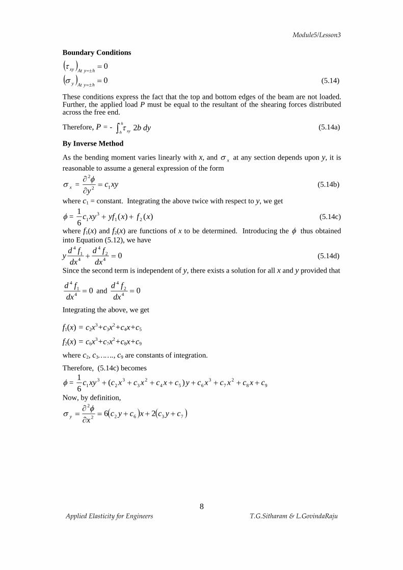
5.3.2 BENDING OF A NARROW CANTILEVER BEAM SUBJECTED TO

END LOAD

Consider a cantilever beam of narrow rectangular cross-section carrying a load P at the end as shown in Figure 5.8.

Figure 5.8 Cantilever subjected to an end load

The above problems may be considered as a case of plane stress provided that the thickness of the beam t is small relative to the depth 2h.

Module5/Lesson3


Boundary Conditions

( ) 0=±= hyAtxyt

( ) 0=±= hyAtys (5.14)

These conditions express the fact that the top and bottom edges of the beam are not loaded. Further, the applied load P must be equal to the resultant of the shearing forces distributed across the free end.

Therefore, P = - ò+

-

h

h xy dyb2t (5.14a)

By Inverse Method

As the bending moment varies linearly with x, and xs at any section depends upon y, it is

reasonable to assume a general expression of the form

xs = xycy 12

2

=¶¶ f

(5.14b)

where c1 = constant. Integrating the above twice with respect to y, we get

f = )()(61

213

1 xfxyfxyc ++ (5.14c)

where f1(x) and f2(x) are functions of x to be determined. Introducing the f thus obtained into Equation (5.12), we have

y 042

4

41

4

=+dx

fddx

fd (5.14d)

Since the second term is independent of y, there exists a solution for all x and y provided that

041

4

=dx

fd and 04

24

=dx

fd

Integrating the above, we get f1(x) = c2x3+c3x2+c4x+c5

f2(x) = c6x3+c7x2+c8x+c9

where c2, c3……., c9 are constants of integration.

Therefore, (5.14c) becomes

f = 982

73

6542

33

23

1 )(61

cxcxcxcycxcxcxcxyc ++++++++

Now, by definition,

( ) ( )73622

2

26 cycxcycxy +++=

¶¶

=fs

Module5/Lesson3


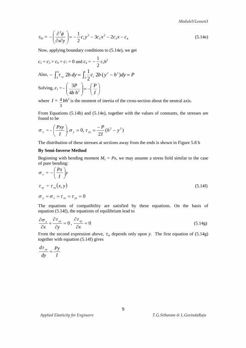
txy = 432

22

1

2

2321

cxcxcycyx

----=÷÷ø

öççè

æ¶¶

¶-

f (5.14e)

Now, applying boundary conditions to (5.14e), we get

c2 = c3 = c6 = c7 = 0 and c4 = 21

- c1h2

Also, ò ò+

- -=-=-

h

h

h

hxy Pdyhybcdyb )(221

2 221t

Solving, c1 = - ÷øö

çèæ-=÷÷

ø

öççè

æIP

hbP

343

where I = 34 bh3 is the moment of inertia of the cross-section about the neutral axis.

From Equations (5.14b) and (5.14e), together with the values of constants, the stresses are found to be

xs = - )(2

,0, 22 yhIP

IPxy

xyy --

==÷øö

çèæ ts

The distribution of these stresses at sections away from the ends is shown in Figure 5.8 b

By Semi-Inverse Method

Beginning with bending moment Mz = Px, we may assume a stress field similar to the case of pure bending:

xs = yI

Px÷øö

çèæ-

xyt = ( )yxxy ,t (5.14f)

0==== yzxzzy ttss

The equations of compatibility are satisfied by these equations. On the basis of equation (5.14f), the equations of equilibrium lead to

0=¶

¶+

¶¶

yxxyx

ts, 0=

¶

¶

xxyt

(5.14g)

From the second expression above, txy depends only upon y. The first equation of (5.14g) together with equation (5.14f) gives

IPy

dy

d xy =t

Module5/Lesson3


or txy = c

IPy

+2

2

Here c is determined on the basis of (txy)y=±h = 0

Therefore, c = - I

Ph2

2

Hence, txy = I

PhI

Py22

22

-

Or txy = - )(2

22 yhI

P-

The above expression satisfies equation (5.14a) and is identical with the result previously obtained. 5.3.3 PURE BENDING OF A BEAM

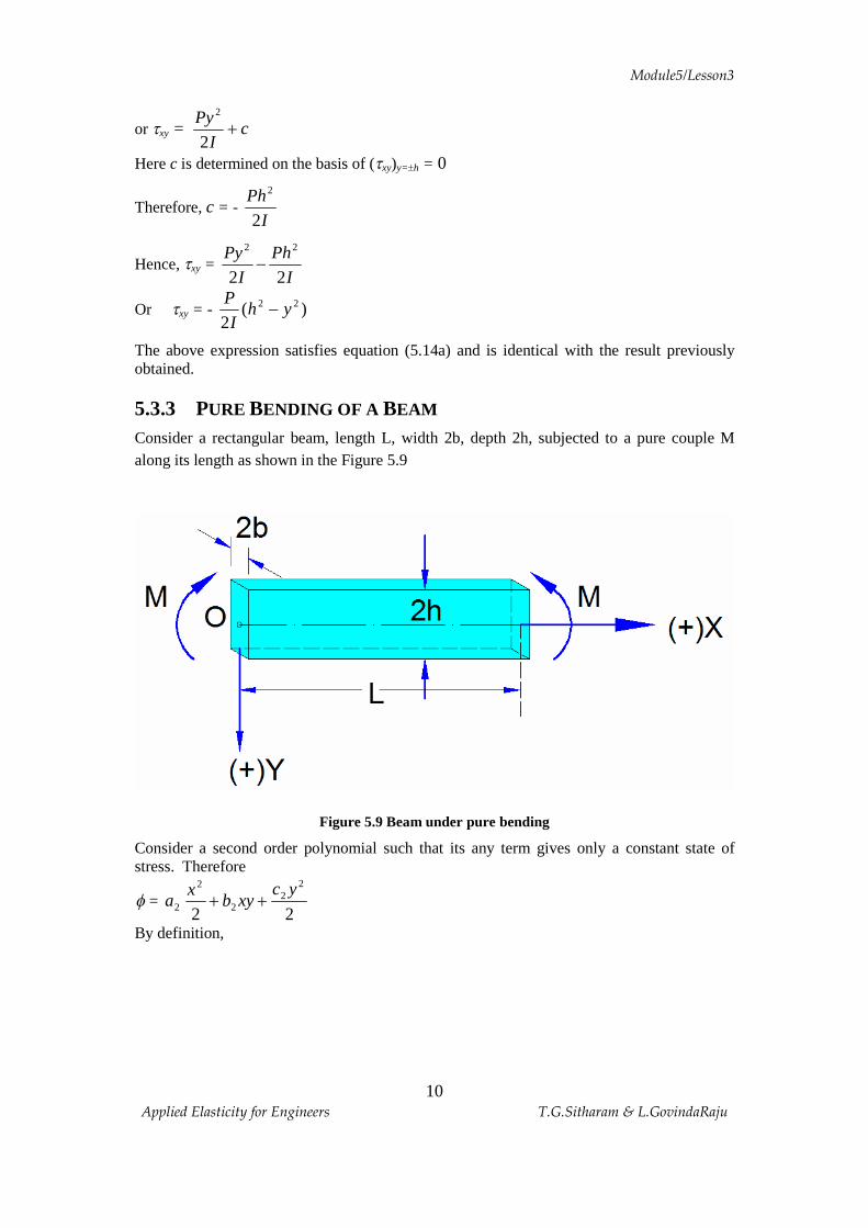
Consider a rectangular beam, length L, width 2b, depth 2h, subjected to a pure couple M along its length as shown in the Figure 5.9

Figure 5.9 Beam under pure bending

Consider a second order polynomial such that its any term gives only a constant state of stress. Therefore

f = 2a22

22

2

2 ycxyb

x++

By definition,

Module5/Lesson3


xs = 2

2

y¶¶ f

, ys = 2

2

x¶¶ f

, txy = ÷÷ø

öççè

æ¶¶

¶-

yxf2

\ Differentiating the function, we get

sx = 2

2

y¶¶ f

= c2, sy = 2

2

x¶¶ f

= a2 and txy = ÷÷ø

öççè

æ¶¶

¶-

yxf2

= -b2

Considering the plane stress case, sz = txz = tyz = 0

Boundary Conditions

(a) At y = ± h, =ys 0

(b) At y = ± h, txy = 0 (c) At x = any value,

2b ò+

-

a

a x ydys = bending moment = constant

\2bx ò+

-

+

-

=úû

ùêë

é=h

h

h

h

yxbcydyc 0

22

2

22

Therefore, this clearly does not fit the problem of pure bending.

Now, consider a third-order equation

f = 6226

33

2323

33 ydxyc

yxbxa

+++

Now, xs = ydxcy 332

2

+=¶¶ f

(a)

ys = a3x + b3y (b)

txy = -b3x - c3y (c)

From (b) and boundary condition (a) above,

0 = a3x ± b3a for any value of x \ a3 = b3 = 0

From (c) and the above boundary condition (b), 0 = -b3x ± c3a for any value of x

therefore c3 = 0 hence, xs = d3y

ys = 0

txy = 0

Obviously, Biharmonic equation is also satisfied.

Module5/Lesson3


i.e., 024

4

22

4

4

4

=¶¶

+¶¶

¶+

¶¶

yyxxfff

Now, bending moment = M = 2b ò+

-

h

h x ydys

i.e. M = 2b ò+

-

h

hdyyd 2

3

= 2bd3 ò+

-

h

hdyy 2

= 2bd3

h

h

y+

-úû

ùêë

é3

3

M = 4bd3 3

3h

Or d3 = 34

3bhM

I

Md =3 where

34 3bh

I =

Therefore, xs = yI

M

Module5/Lesson3


5.3.4 BENDING OF A SIMPLY SUPPORTED BEAM BY A DISTRIBUTED

LOADING (UDL)

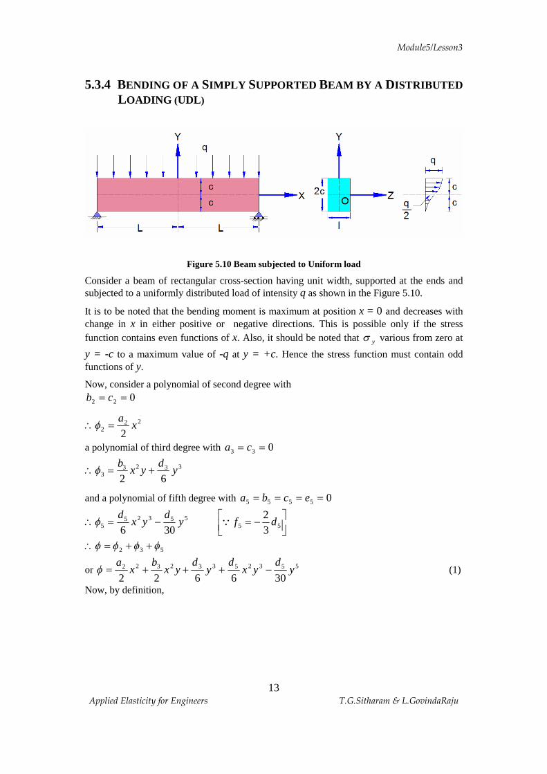
Figure 5.10 Beam subjected to Uniform load

Consider a beam of rectangular cross-section having unit width, supported at the ends and subjected to a uniformly distributed load of intensity q as shown in the Figure 5.10.

It is to be noted that the bending moment is maximum at position x = 0 and decreases with change in x in either positive or negative directions. This is possible only if the stress function contains even functions of x. Also, it should be noted that ys various from zero at

y = -c to a maximum value of -q at y = +c. Hence the stress function must contain odd functions of y.

Now, consider a polynomial of second degree with 022 == cb

222 2

xa

=\f

a polynomial of third degree with 033 == ca

33233 62

yd

yxb

+=\f

and a polynomial of fifth degree with 05555 ==== ecba

úûù

êëé -=-=\ 55

553255 3

2306

dfyd

yxd Qf

532 ffff ++=\

or 55325332322

306622y

dyx

dy

dyx

bx

a-+++=f (1)

Now, by definition,

Module5/Lesson3


÷øö

çèæ -+=

¶¶

= 32532

2

32

yyxdydyx

fs (2)

35322

2

3y

dyba

xy ++=¶¶

=fs (3)

253 xydxbxy --=t (4)

The following boundary conditions must be satisfied. (i) ( ) 0=

±= cyxyt

(ii) ( ) 0=+= cyys

(iii) ( ) qcyy -=

-=s

(iv) ( )ò+

-±= =

c

cLxx dy 0s

(v) ( )ò+

-±=

±=c

cLxxy qLdyt

(vi) ( )ò+

-±= =

c

cLxx ydy 0s

The first three conditions when substituted in equations (3) and (4) give 02

53 =-- cdb

03

3532 =++ c

dcba

qcd

cba -=-- 3532 3

which gives on solving

3532 43

,43

,2 c

qd

cq

bq

a -==-=

Now, from condition (vi), we have

ò+

-

=úû

ùêë

é÷øö

çèæ -+

c

c

ydyyyxdyd 032 32

53

Simplifying,

÷øö

çèæ --= 22

53 52

hLdd

Module5/Lesson3


÷ø

öçè

æ -=52

43

2

2

hL

hq

÷øö

çèæ --÷

ø

öçè

æ -=\ 32

32

2

32

43

52

43

yyxhq

yhL

hq

xs

3

3443

2y

hq

yhqq

y -+÷øö

çèæ-=s

2

343

43

xyhq

xhq

xy +÷øö

çèæ-=t

Now, ( ) 333

32

128

1221

hhh

I ==´

=

where I = Moment of inertia of the unit width beam.

( ) ÷ø

öçè

æ -+-=\532

2322 yhy

Iq

yxLI

qxs

÷ø

öçè

æ +-÷øö

çèæ-= 32

3

32

32hyh

yI

qys

( )22

2yhx

Iq

xy -÷øö

çèæ-=t

5.3.5 NUMERICAL EXAMPLES

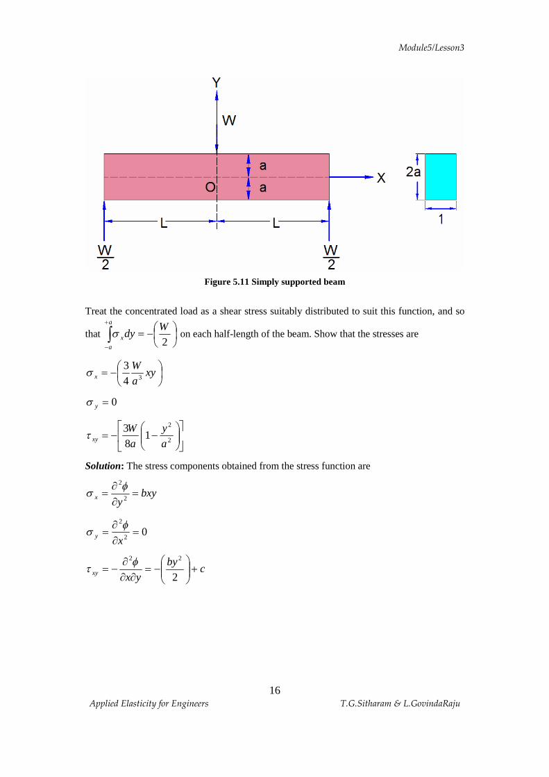
Example 5.1 Show that for a simply supported beam, length 2L, depth 2a and unit width, loaded by a concentrated load W at the centre, the stress function satisfying the loading condition

is cxyxyb

+= 2

6f the positive direction of y being upwards, and x = 0 at midspan.

Module5/Lesson3


Figure 5.11 Simply supported beam

Treat the concentrated load as a shear stress suitably distributed to suit this function, and so

that ò+

-

÷øö

çèæ-=

a

a

x

Wdy

2s on each half-length of the beam. Show that the stresses are

÷øö

çèæ-= xy

aW

x 343s

0=ys

úû

ùêë

é÷÷ø

öççè

æ--= 2

2

183

ay

aW

xyt

Solution: The stress components obtained from the stress function are

bxyyx =

¶¶

=2

2fs

02

2

=¶¶

=xy

fs

cby

yxxy +÷÷ø

öççè

æ-=

¶¶¶

-=2

22ft

Module5/Lesson3


Boundary conditions are

(i) ayfory ±== 0s

(ii) ayforxy ±== 0t

(iii) ò+

-

±==-a

axy Lxfor

Wdy

2t

(iv) ò+

-

±==a

ax Lxfordy 0s

(v) ò+

-

±==a

ax Lxforydy 0s

Now,

Condition (i) This condition is satisfied since 0=ys

Condition (ii)

cba

+÷÷ø

öççè

æ-=

20

2

2

2bac =\

Condition (iii)

( )ò+

-

--=a

a

dyyabW 22

22

÷÷ø

öççè

æ--=

32

22

33 a

ab

÷÷ø

öççè

æ-=\

32

2

3baW

or ÷øö

çèæ-= 34

3aW

b

and ÷øö

çèæ-=

aW

c83

Condition (iv)

Module5/Lesson3


ò+

-

=÷øö

çèæ-

a

a

xydyaW

043

3

Condition (v)

ò+

-

=a

ax ydyM s

ò+

-

÷øö

çèæ-=

a

a

dyxyaW 2

343

2

WxM =\

Hence stress components are

xyaW

x ÷øö

çèæ-= 34

3s

0=ys

÷øö

çèæ-÷÷

ø

öççè

æ=

aWy

aW

xy 83

243 2

3t

úû

ùêë

é÷÷ø

öççè

æ--=\ 2

2

183

ay

aW

xyt

Example 5.2

Given the stress function ÷øö

çèæ

÷øö

çèæ= -

zx

zH 1tanp

f . Determine whether stress function f is

admissible. If so determine the stresses.

Solution: For the stress function f to be admissible, it has to satisfy bihormonic equation. Bihormonic equation is given by

02 4

4

22

4

4

4

=¶¶

+¶¶

¶+

¶¶

zzxxfff

(i)

Now, úû

ùêë

é÷øö

çèæ+÷

øö

çèæ

+-=

¶¶ -

zx

zxxzH

z1

22 tanp

f

( )[ ]32322

2222

2

21

xxzxxzxzzx

Hz

----+

÷øö

çèæ=

¶¶

pf

( ) úúû

ù

êêë

é

+÷øö

çèæ-=

¶¶

\ 222

3

2

2 2

zx

xHz pf

Module5/Lesson3


Also, ( ) úúû

ù

êêë

é

+=

¶¶

322

3

3

3 8

zx

zxHz pf

( ) úúû

ù

êêë

é

+

-=

¶¶

422

235

4

4 408

zx

zxxHz pf

( ) úúû

ù

êêë

é

+

-÷øö

çèæ-=

¶¶¶

322

423

2

3 32

zx

xzxHxz p

f

( ) úúû

ù

êêë

é

+

--=

¶¶¶

422

5423

22

4 82464

zx

xxzzxHxz p

f

Similarly,

( )úûù

êë

é+

=¶¶

22

2

zxzH

x pf

( ) úúû

ù

êêë

é

+÷øö

çèæ-=

¶¶

222

2

2

2 2

zx

xzHx pf

( )( ) ú

úû

ù

êêë

é

+

-=

¶¶

322

222

3

3 32

zx

zxz

Hx pf

( ) úúû

ù

êêë

é

-

-=

¶¶

422

234

4

4 2424

zx

zxxzHx pf

Substituting the above values in (i), we get

( )[ 5423234

422824642424

14xxzzxzxxz

zx--+-

+p] 0408 235 =-+ zxx

Hence, the given stress function is admissible. Therefore, the stresses are

( ) úúû

ù

êêë

é

+÷øö

çèæ-=

¶¶

= 222

3

2

2 24

zx

xzx pfs

( ) úúû

ù

êêë

é

+÷øö

çèæ-=

¶¶

= 222

2

2

2 24

zx

xxy pfs

and ( ) úúû

ù

êêë

é

+÷øö

çèæ-=

¶¶¶

= 222

22 24

zx

zxzxxy p

ft

Module5/Lesson3


Example 5.3

Given the stress function: ( )zdxzdF

2323 -÷

øö

çèæ-=f .

Determine the stress components and sketch their variations in a region included in z = 0, z = d, x = 0, on the side x positive.

Solution: The given stress function may be written as

33

22

23xz

dF

xzdF

÷øö

çèæ+÷

øö

çèæ-=f

xzd

FdFx

z÷øö

çèæ+÷

øö

çèæ-=

¶¶

\322

2 126f

and 02

2

=¶¶

xf

also 232

2 66z

dF

dFz

zx÷øö

çèæ+÷

øö

çèæ-=

¶¶¶ f

Hence xzd

FdFx

x ÷øö

çèæ+÷

øö

çèæ-=

32

126s (i)

0=zs (ii)

232

2 66z

dF

dFz

zxxz ÷øö

çèæ+÷

øö

çèæ-=

¶¶¶

-=jt (iii)

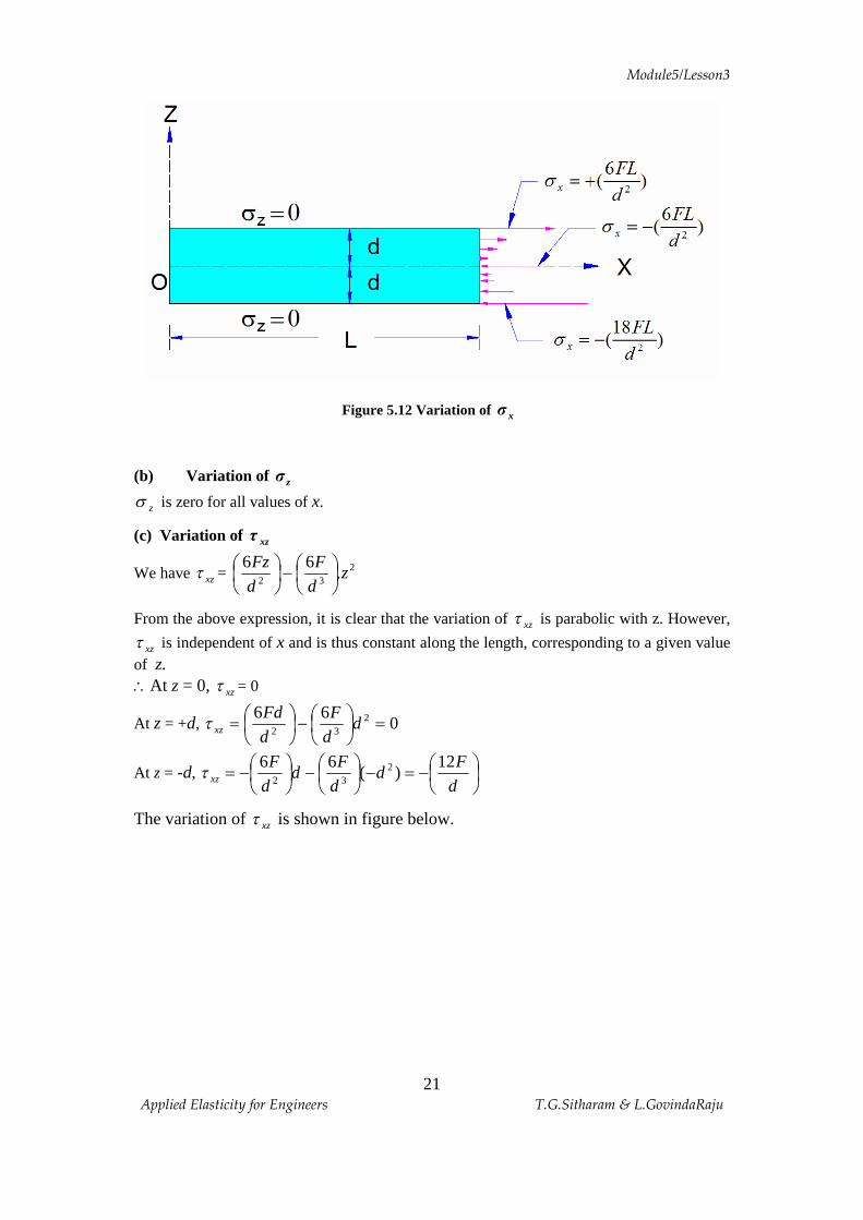
VARIATION OF STRESSES AT CERTAIN BOUNDARY POINTS (a) Variation of xσ

From (i), it is clear that xs varies linearly with x, and at a given section it varies linearly with z. \ At x = 0 and z = ± d, xs = 0

At x = L and z = 0, ÷øö

çèæ-= 2

6dFL

xs

At x = L and z = +d, 232

6126dFL

Ldd

FdFL

x =÷øö

çèæ+÷

øö

çèæ-=s

At x = L and z = -d, ÷øö

çèæ-=÷

øö

çèæ-÷

øö

çèæ-=

232

18126dFL

Ldd

FdFL

xs

The variation of xs is shown in the figure below

Module5/Lesson3


Figure 5.12 Variation of xσ

(b) Variation of zσ

zs is zero for all values of x.

(c) Variation of xzτ

We have xzt = 232 .

66z

dF

dFz

÷øö

çèæ-÷

øö

çèæ

From the above expression, it is clear that the variation of xzt is parabolic with z. However,

xzt is independent of x and is thus constant along the length, corresponding to a given value of z. \At z = 0, xzt = 0

At z = +d, 066 2

32 =÷øö

çèæ-÷

øö

çèæ= d

dF

dFd

xzt

At z = -d, ÷øö

çèæ-=-÷

øö

çèæ-÷

øö

çèæ-=

dF

ddF

ddF

xz

12)(

66 232t

The variation of xzt is shown in figure below.

Module5/Lesson3


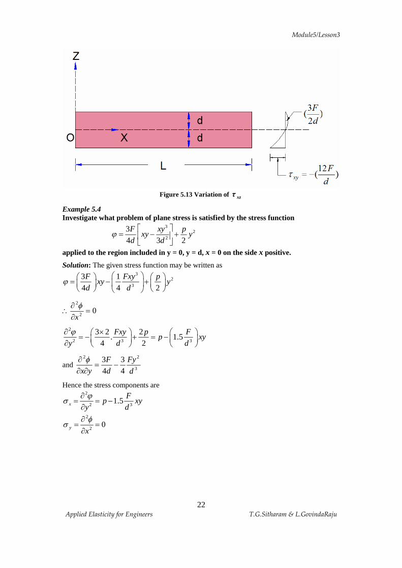
Figure 5.13 Variation of xzτ

Example 5.4 Investigate what problem of plane stress is satisfied by the stress function

32

2

34 3 2F xy p

xy yd d

jé ù

= - +ê úë û

applied to the region included in y = 0, y = d, x = 0 on the side x positive.

Solution: The given stress function may be written as 3

23

3 14 4 2F Fxy p

xy yd d

jæ öæ ö æ ö= - +ç ÷ç ÷ ç ÷

è ø è øè ø

02

2

=¶¶

\xf

2

2 3 3

3 2 2. 1.5

4 2Fxy p F

p xyy d dj¶ ´æ ö æ ö= - + = -ç ÷ ç ÷¶ è ø è ø

and 3

22

43

43

dFy

dF

yx-=

¶¶¶ f

Hence the stress components are 2

2 31.5x

Fp xy

y djs ¶

= = -¶

02

2

=¶¶

=xy

fs

Module5/Lesson3


dF

dFy

yxxy 43

43

3

22

-=¶¶

¶-=

ft

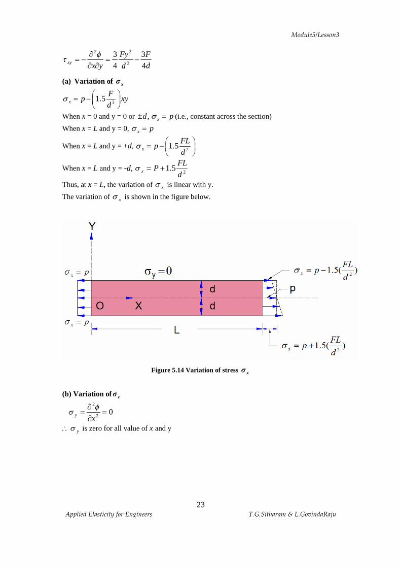
(a) Variation of xσ

31.5x

Fp xy

ds æ ö= - ç ÷

è ø

When x = 0 and y = 0 or , xd ps± = (i.e., constant across the section)

When x = L and y = 0, x ps =

When x = L and y = +d, 21.5x

FLp

ds æ ö= - ç ÷

è ø

When x = L and y = -d, 2

5.1dFL

Px +=s

Thus, at x = L, the variation of xs is linear with y.

The variation of xs is shown in the figure below.

Figure 5.14 Variation of stress xσ

(b) Variation of zσ

02

2

=¶¶

=xy

fs

\ ys is zero for all value of x and y

Module5/Lesson3


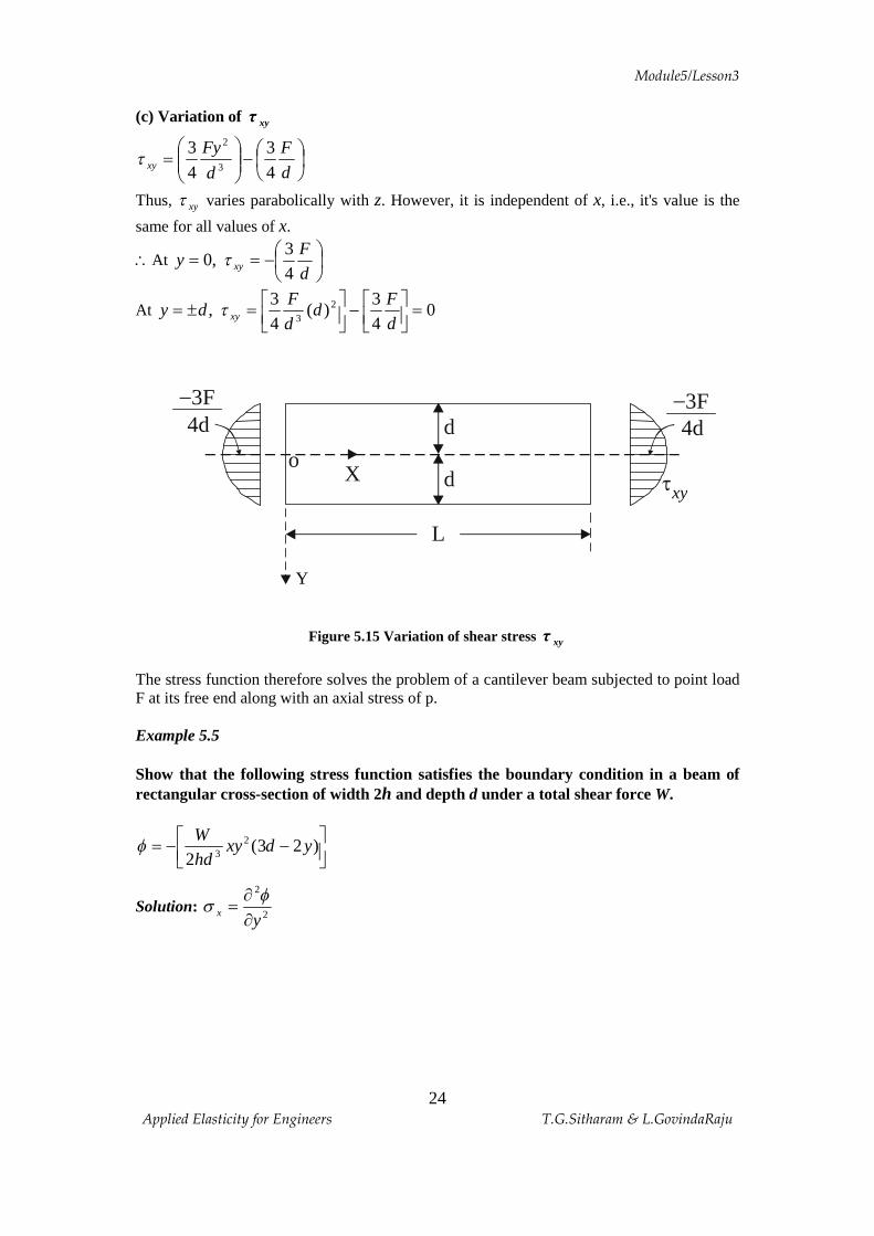
(c) Variation of xyτ

÷øö

çèæ-÷÷

ø

öççè

æ=

dF

d

Fyxy 4

343

3

2

t

Thus, xyt varies parabolically with z. However, it is independent of x, i.e., it's value is the

same for all values of x.

\At ÷øö

çèæ-==

dF

y xy 43

,0 t

At 043

)(43

, 23

=úûù

êëé-úû

ùêëé=±=

dF

ddF

dy xyt

Figure 5.15 Variation of shear stress xyτ

The stress function therefore solves the problem of a cantilever beam subjected to point load F at its free end along with an axial stress of p. Example 5.5 Show that the following stress function satisfies the boundary condition in a beam of rectangular cross-section of width 2h and depth d under a total shear force W.

úûù

êëé --= )23(2

23 ydxy

hdWf

Solution: 2

2

yx ¶¶

=fs

Y

d

d

L

X o

t xy

- 3F 4d

- 3F 4d

Module5/Lesson3


Now, [ ]23

662

xyxydhdW

y--=

¶¶f

[ ]xyxdhdW

y126

2 32

2

--=¶¶ f

[ ]xyxdhdW

x 633

--=\s

02

2

=¶¶

=xy

fs

and yxxy ¶¶

¶-=

ft2

= [ ]23

662

yydhdW

-

= [ ]23

33 yydhdW

-

Also, 02

22

4

4

4

4

44 =ú

û

ùêë

é¶¶¶

+¶¶

+¶¶

=Ñ ffyxyx

Boundary conditions are

(a) dandyfory 00 ==s

(b) dandyforxy 00 ==t

(c) LandxforWdyhd

xy 0.2.0

==òt

(d) WLMLxandxfordyhMd

x ===== ò ,00.2.0

s

(e) Lxandxfordyyhd

x ===ò 00..2.0

s

Now, Condition (a)

This condition is satisfied since 0=ys

Condition (b)

[ ] 033 223

=- ddhdW

Module5/Lesson3


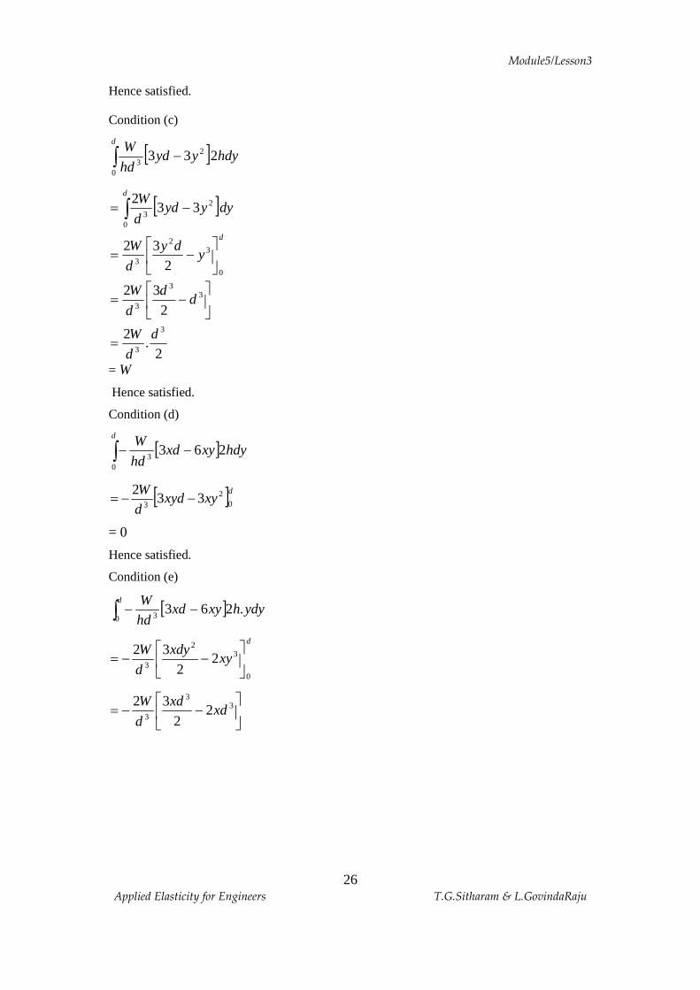
Hence satisfied.

Condition (c)

[ ] hdyyydhd

Wd

2330

23ò -

[ ]dyyydd

Wd

ò -=0

23

332

d

ydy

dW

0

32

3 232

úû

ùêë

é-=

úû

ùêë

é-= 3

3

3 232

dd

d

W

2.

2 3

3

ddW

=

= W

Hence satisfied.

Condition (d)

[ ] hdyxyxdhd

Wd

2630

3ò --

[ ]dxyxyd

dW

02

3 332

--=

= 0

Hence satisfied.

Condition (e)

[ ] ydyhxyxdhdWd

.2630 3ò --

d

xyxdy

dW

0

32

32

232

úû

ùêë

é--=

úû

ùêë

é--= 3

3

32

232

xdxd

d

W

Module5/Lesson3


úûù

êëé--= 3

3 212

xddW

Wx=

Hence satisfied

Documents

Lec Diffvcvvbv