NASA Contractor Report 187601

leASE Report No. 91-55

leASE

NAsA-elf- IfZ &0/

NASA-CR-187601 19910021436

RECTILINEAR PARTITIONING OF IRREGULAR DATA PARALLEL COMPUTATIONS

David M. Nicol

Contract No. NASI-18605 July 1991

Institute for Computer Applications in Science and Engineering NASA Langley Research Center Hampton, VIrginia 23665-5225

Operated by the Universities Space Research Association

NI\SI\ National Aeronautics and Space Administration

Langley Research Center Hampton, Virginia 23665-5225

111111111111111111111111111111111111111111111 NF00790

LIBRARY COpy SEP I 81991

LANGLEY RESEARCH CENTER LIBRARY NASA

HAMPTON VIRGINIA

https://ntrs.nasa.gov/search.jsp?R=19910021436 2018-07-14T05:42:42+00:00Z

Rectilinear Partitioning of Irregular Data Parallel Computations

David M. Nicol*

College of Wilham and Mary

Abstract

ThIS paper descrIbes new mappmg algorIthms for domam-orIented data-parallel computa­tIOns, where the workload IS dIstrIbuted Irregularly throughout the domam, but exhIbIts locahzed commUUlcatIOn patterns We conSIder the problem of partItIonmg the domam for parallel pro­cessmg m such a way that the workload on the most heavIly loaded processor IS mmlmlzed, subject to the constramt that the partitIOn be perfectly rectIlInear Rectilmear partItIOns are useful on archItectures that have a fast local mesh network and a relatIvely slower global net­work, these partItIOns heUrIstIcally attempt to ma.'Clmize the fractIOn of commumcatIon carrIed by the local network ThIS paper prOVIdes an Improved algOrIthm for findmg the optImal par­titIOn m one dImenSIOn, new algOrIthms for partitIOnmg 111 two dImenSIOns, and shows that optimal partitIOnmg m three dImenSIOns IS NP-complete We dISCUSS our applIcatIOn of these algOrIthms to real problems

·Thls research was supported In part by the Army AVlOlIlCS Research and Development ACtIVIty through NASA grant NAG-I-787, In part by NASA grant NAG-I-U32, and In part by NSF Grant ASe 8819373

1 Introduction

One of the most important problems one must solve m order to use parallel computers is the mappmg of the workload onto the architecture. This problem has attracted a great deal of attention m the literature, leading to a number of problem formulations. One often views the computation III terms of a graph, where nodes represent computations and edges represent communication; for example, see [2]. Mapping means assigning each node to a processor; this is equivalent to partitioning the nodes of the graph, wIth the tacit understanding that nodes in a common partition

set are assigned to the same processor. We will use the terms interchangeably. A common mapping problem formulation views the architecture as a graph whose nodes are processors and whose edges identify processors able to commUnIcate dIrectly. The dzlatzon of a computation graph edge ( u, v) IS the minimum dIstance (in the processor graph) between the processors to whIch u and

v are respectively assigned. The dilation of the graph itself is the maximum dilation among all computation graph edges. Dilation is a measure of how well the mappmg preserves locality between

nodes in the mapped computation graph. Results concerning the minimizatIOn of dilation can be

found in [4, 9, 16,21], and their references Another formulation (the one we study) dllectly models execution time of a data parallel com­

putatIOn as a function of the chosen mapping, and attempts to find a mapplllg that minimizes the execution time. Workload may again be represented as a graph, with edges representing data com­munication, e.g., the stencils used in some partIal differential equation solvers [18]. In its simplest form each node is assumed to have unit execution weight; more general forms permit nodes to have individual weights. Nodes are mapped to processors in such a way that each processor's sum of node weights is approximately the same, for example, see [1, 3, 19]. A rigorous treatment of partitioning three dimenSIOnal finite-difference and finite-element domains is found in [23]; unlIke our treatment

here, the shape of the subdomallls are not a consideration. MlllimIzation of communication costs subject to load-balanclllg constraints is considered in [6], other formulations use sImulated anneal­

lllg or neural networks to minimize an "energy" function that heUrIstIcally quantifies the cost of the partition [7]. Other lllteresting formulations conSIder mapping highly structured computatIOns onto pIpelmed multiprocessors[14], and mapping systolic algouthms onto hypercubes [10].

This paper considers the Rectzlmear Partztzonmg Problem (RPP). find an optimal rectzimear

partition of a domalll contallling ineguially WeIghted workload. One may view the workload as being concentrated at discrete coordinates within the domalll, alternatively one may represent the domain's workload in a workload matrIx, each of whose elements represents all the workload withlll a rectangular fixed-SIzed region of the domalll. A domain with irregularly distributed dIscrete workload can always be transformed lllto a workload matrix, our problem formulatIOn WIll thus be stated in terms of the matrix view. A rectilinear partition of a workload matrix requires each partItion element to be an applopriately dimenSIOned "rectangle" whose dlmj:!nsions exactly match that of each neighbor at each face. "Rectangles" in one dImension are intervals; a "rectangle" in three dimensions is a rectangular solId. The cost of a rectangle IS the sum of all workload WIthin ItS boundarIes; the cost of the partition is the maximum cost among all Its rectangles. The idea

1

H-I- ..

" , ,-,- 1 r-r- "T f-i-I- ....

-I-t- ........ -I-t- ........ -I-t---'- --'-, , , , , , , , , , -,-.1-,-,-.1-,-,-•

-r-r"T,-r-r"T,-r-r -I- t- ........ -1- t- ........ -1- t-

--< , , ,-,- , """"" 1 -,-.1-,-,-.1-,-,-.

, , , , , , , , -,-,-.1-,-,-.1 ,-r-r"T,-r-r"T ....-I-t- ........ -I-t- .... , , , , , , , , -,-,-.1-,-,-.1

~-I- .... -I-t- ........ -I-t- ........ -I-t- .... -I-t- ........ -I-t- .... ~_L ~ _L~~~_L~~~_L~ ~_L~~~_L~~ r!-'- 1 _'- 1.1_'_'- 1.1_'_'_ 1. _,_,_ 1.1_'_'- 1.1

FIgure 1: Two dImensIOnal 4 X 4 rectIlInear partition of a workload matrix representmg a two­

dimensional domain

is to let the weight of a rectangle be the time reqUIred to execute its implicitly assigned workload on a processor. The maximum such defines the computation's finishmg time (or its inverse defines the processmg rate) when each rectangle IS assIgned to a dIfferent processor. Figure 1 illustrates a rectilmear partition in two dImensions.

RPP arises when executmg physIcally-oriented numencal computatIOns on certain types of mesh-connected multIprocessors. For example, some computatIOns are based on grids that discretIze

a one, two or three dimensional field for numerical solutIOn. An n X m workload matrix can be constructed by pre-aggregatmg adjacent gnd points to create a rectangular structure; alternatively, one may chose nand m so large that at most one gnd point is represented in one cell of the n X m domam. RPP IS motIvated by parallel archItectures that support very fast "local" communicatIOn over a mesh network, and sigmficantly slower "global" communicatIOn. The Connection Machine prOVIdes an example: the speed differentIal between commumcation using the local network and the

global router is roughly a factor of SIX on problems with regular communication patterns [22]. It can be worse if the global network suffers significant contention. Smce communication requirements m domain-oriented computations are often localIzed in space, rectilInear partItIOns will tend to maximIze the volume of communication which can use the fast mesh network.

It is pOSSIble to partition a domam with irregularly dIstributed discrete workload into quadrilat­erals whose faces match exactly, as do rectilInear partitions. Such partItIOns will have the desirable

localIty of communication properties we seek. However, rectIlmear partitIOns have the advantage of bemg expressed simply. One benefit is that one can always compute the processor Id of a pOInt (x, y) with whom wishes to communicate: a binary search on the hst of cuts m the X dimenSIOn establishes the X processor cOOldmate of (x, y)'s processor, another search establIshes the Y pro­cessor coordinate. SimpliCIty of expreSSIOn also ImplIes simplICIty of construction. There is some advantage to choosing N + M - 2 cuts instead of choosmg (N - 1) X (M - 1) cuts. Finally, the

2

mathematical regulanty of rectIlmear partitions make them mterestmg objects in theIr own nght. We consider partitioning m one, two, and three dImensions. It should be noted that a three di­

mensional domain can always be partitioned for a two or one dimenSIOnal processor array; likewise,

a two dimensional domam can be partItIOned for a one dimenSIOnal processor array. Thus, the par­titIOnmg dimension describes the communication topology of the target archItecture. A dIstmction can be made between processor meshes that directly connect dIagonally adjacent processors, and those that don't. The algonthms we develop here are pnmarily concerned wIth the latter. They

may be used on more fully connected meshes, but do not attempt to take advantage of the extra

connectivity. RPP is a challenging problem, as it is similar to certain NP-complete problems, but is also

similar to problems with polynomial complexity. It is already known that the one-dimensional problem can be solved in polynomial time [3, 5, 17]. Our first result IS to improve upon the best published 1D algonthm to date, for the case when the computation's size greatly exceeds the number of processors. Next we consider RPP in two dimenSIOns. We show that If the partition m one dimension (say x) is fixed, then the optimal partItIoning in the other dImension can be found in

polynomial time. ThIS result has at least two applicatIOns. First, it can be used to find the optimal 2D rectilinear partition; one simply generates all partitions in one dimension, and finds, for each,

the optImal partitionmg in the other. While this procedure is correct, it has unreasonably hIgh complexity. For this reason we develop a 2D zteratzve refinement heunstIc based on our ability to find conditIOnally optimal partItIOns. During each Iteration, one finds the optImal partitIOnmg in one dimenSIOn, given a fixed partition in the other. The next iteration uses the solutIOn just found as the fixed partitIOn, and optimally solves in the other dimenSIOn. One then iterates untIl the partition stops changing. The procedure is guaranteed to converge monotonically to a local mmlmum in the

solution space. We discuss application of this technique to two-dimensional problems arising in fluid dynamics calculations, and compare the quality of solutIons produced by the heuristic WIth solutions

produced by algorithms having fewer restrictions on the partitioning, e.g., binary dissection. We find that rectilinear partitIOns can achieve better performance than the other methods, especially

when the grid edges are onented in two orthogonal dIrections, or when global communication is an order of magnitude slower than local commulllcation Our last contnbution is to show that the problem of finding an optimal rectilinear partition m three dimenSIons is NP-complete.

The remainder of thIS paper is orgalllzed as follows. In SectIOn §2 we introduce some notation

and develop the cost functIOn we WIsh to minimIze. In SectIOn §3 we gIve an improved solution to RPP in one dimenSIOn. SectIOn §4 exammes RPP in two dimensions, and Section §5 proves

the NP-completeness of findmg optimal three-dimensional partItIOns. SectIOn §6 summarizes our

results

2 Preliminaries

This section introduces some notatIOn used throughout the paper. The discussion to follow speaks of the two dimensional partitioning problem; the extension to three dImensions is immediate, and

3

the projection to one dImension simply involves droppmg notational dependence on indices in one

dimension. We define the partitioning problem as follows. Consider an n X m load matrzx {L I ,]}, where each

entry L I ,] ~ 0 represents the cost of executing some workload. For example, we might create a load matrix from a discretized domain by prepartitioning the domain into many rectangular work pzeces,

and assign load value L I ,] to work pIece WI,], based on the number of grId points and edges defined within WI,]" In the limit, we may prepartItion the domain so finely that a work piece represents at

most one grid pomt and Its edges. Our problem IS to partition the load matrix for execution on an N x M array of processors,

as follows. A partition IS defined to be a pair of vectors (R, C), where R is an ordered set of row indices R = (ro,r}, ... ,rN), C is an ordered set of column indices C = (CO,Cl, ... ,CM), and we

understand that ro = Co = 0, rM = m, and CN = n. Given (R, C), the executIOn load on processor PI,] IS the sum of the weights of all the work pieces Wx,y with r,-l < x ~ r" and C]-l < Y ~ c].

ThIS IS gIven by r,

X,,](R,C) = L

We take the overall cost of the partItion to be the maximal execution load assigned to any processor:

7r(R, C) = max {XI,](R, Cn. all, and J

This cost is known as the bottleneck value for the partitIOn. Our object IS to find partition vectors

Rand C that minimize the bottleneck value. We have chosen not to include explicit communication costs in this model. This is a largely

practIcal decision The data communication inherent in a computational problem tends to be pro­portIOnal to execution costs. This means that by balancmg the executIOn load we will have greatly

balanced the commulllcationioad also, at least if the bandwidth of the netwOlk IS high enough for us to ignore contention. It is also true that the execution weights L,,] are only estimates to be­gin with; it seems unlikely that a more complIcated model will find significantly better partitions. Finally, we are assuming that rectIlinear partitioning is desirable because local communication IS much cheaper than global communicatIOn. If we can ensure that the partition supports local communication we will have gone a long way towards mmimlzmg communication overhead. Our empirical study discussed in §4.5 bears out this intuition.

3 One Dimensional Partitioning

RPP in one dimenSIOn has been extensively studied as the chams-on-chams partitioning problem [3, 5, 11, 12, 17]. we are given a linear sequence of work pIeces (called modules), and wish to partition the sequence for executIOn on a linear array of processors. Until recently, the best pub­

lished algorithm found the optimal partitIOning in O(Mmlogm) time, where M is the number of processors and m is the number of modules. This solutIOn and those developed in [11] and [17] all

4

mvolve repeatedly calling a probe function. A recently discovered dynamic programming formula­

tion [5] reduces the complexity further to O(Mm). The solutIOn we present has a complexity of O(m + (Mlogm)2), which is better than O(Mm) when M = O(mfloi' m). This solutIOn is also based on a probe function, which we now discuss in more detail.

In one dimension we are to partitIOn a chain of modules WI, ••• , Wm with weights L1 , • •• , Lm into M contiguous subchains. We use a function probe, which accepts a bottleneck constramt W

and determines whether any partition exists with bottleneck value W', where W' ~ W. Candidate

constraints all have the form W,,] = I:i=, Lk, because we know that the optimal cost is defined by the load we place on some processor. If we precompute the m sums WI,] (J = 1, ... , m), then any

candIdate value W,,] can be generated in 0(1) time using the relationship W,,] = WI,] - W1,,-1. Given bottleneck constraint W, probe attempts to construct a partition with a bottleneck

value no greater than W. The first processor must contain the first module; probe finds the largest mdex tl such that Wl,'l ~ W, and assigns modules 1 through tl to the first processor. Because the sums WI,] increase in), tl can be found WIth a binary search It follows that the first module in the second processor is Wll+!. probe then loads the second processor with the longest

subcham beginning WIth W'l+! that does not overload the processor. This process contmues until either all modules have been assigned, or the supply of processors IS exhausted. In the former case we know that a feaSIble partition with weight no greater than W exists. In the latter case we know that this greedy approach does not produce a feaSIble partitIOn. However, it has been shown (and mdeed is qUite straightforward to see) that the greedy approach will find a solutIOn with cost no greater than W If any solution eXists With cost no greater than W. Smce the loading of each

processor requires only a binary search, the cost of one probe call is O( M log m). All solutions based on probe search the space of bottleneck constraints for the minimal one, say

Wopt , such that probe{Wopt ) = true. The partItion probe generates given bottleneck constraint W opt is optimal. The solution in [17] examines no more than 4m candidate constraints, which gives

the ID partitioning problem an overall time compleXity of O{Mmlogm). As argued by Iqbal[ll], another easy way to probe is to compute the sum of all workload in the domain, say Z, and choose a discretizatIOn length f. One may then conceptually discretize the interval [0, Z] into Z / € constraints, and use a binary search to find the minimum feaSible constraint. This approach has a complexity of O(M 10g(Z/€) logm), although the cost of a partition it finds IS guaranteed only to be WIthin € of optimal. The only disadvantage of this method occurs when log(Z/€) is large relative to m, m which case one may choose to search more cleverly. Towards this end we next develop the paper's first contnbution, a searching technique that finds the optimal partition after only O(Mlogm) probe calls l .

Let Wopt be the minimal constraint for which probe returns value true. The new search strategy exploits the following structure of an optimal solution constructed by probe. Suppose

processor F is the first processor assigned a load whose weight is exactly H'opt. The loads on all processors 1 through t - 1 must be strictly less than Wopt , and hence their loads are not feasible

lThlS result was ongmally observed by Iqbal (pnvate commumcahon) We present an mdependently dlscovered proof (and algonthm) winch easlly extends to a 2D problem

5

bottleneck constraInts. However, the greedy constructIOn process ensures that the load on each processor up to F is as large as possible. For example, processor 1 is loaded with the longest subchain, beginning with WI, whose weight does not exceed Wopt • For any W' < Wopt we have

probe(W') = false; let Zl be the largest index such that probe(W1,tl) = false. Consider the relationships

If Wopt < W1 ,tl+! (Le., if 1 ~ F) then modules 1 through Zl will be assigned to processor 1, otherwise module Zl + 1 will also be assigned to 1. Supposing that 1 < F, the sub chain assigned to processor 2 begins with module Wt1+1; define i2 to be the largest index for which probe(Wt1 +!,t2) = false. Under the greedy assignment, processor 2's last module is either wt2 or wt2 +!, depending on whether F = 2. We may carry out this process for each processor: given zJ' zJ+! is the largest index for

which probe(WtJ+!,tJ+l) = false. For each zJ define wJ = WtJ _ 1+!,tJ +!. From the discussion above it is apparent that when J ~ F, zJ is the first module assigned to processor J under the optimal greedy partition. wJ is the smallest feasible constraint arising from any sub chain beginning with

module wIJ • Therefore, Wopt = WF. Furthermore, each w) for J > F is a feasible constraint, and hence must be at least as large as Wopt • This proves the following lemma.

Lemma 1 Let W opt be the minzmal Jeaszble bottleneck wezght. Then W opt = minl~)~M{WJ}.

An important point is that the defimtIOns of the Z3 's and wJ's in no way depend on knowledge of either F or Wopt • We may discover Wopt by generating each constraint w" and choOSIng the least. In order to find Zl (and hence WI) we need to search the space of all weights having the form WI,). As we have already seen, this space can be searched with only O(1ogm) calls to probe. Each

probe call costs O(Mlogm)j the cost of finding WI is thus O(M log2 m). Similarly, given Zb we find Z2 using a binary search over all weights of the form W t1 +1,J' and so on. As there are M such w/s

to compute, the overall cost of the computation is O(m + (M log m?), where an obligatory O(m) cost is added to account for preprocessing costs. This complexity is better than O(Mm) whenever

M = O(m/log2 m), showing that the strategy IS most useful when there are many modules to be processed relative to processors. TIllS is exactly the situatIOn we face when partItIOning large numerical problems. One of the more useful applications of the new algorithm wIll be as part of an approach for solving two dImensional problems, our next tOPIC.

4 Two Dimensional Partitioning

Next we turn to partitioning in two dImensions. Our discussion has three parts. FIrst we provide

some contrast by dIscussing a closely related 2D partItIOning problem which is NP-complete. We then return to our original 2D problem, and descnbe an algorIthm that takes a given fixed column (alternately, row) partition, and finds the optimal partitioning of the rows (alternately, columns) in polynomial time. This result can be used to find an optimal 2D partition, albeit with exponential

complexity when Nand M are problem parameters .. We describe a heuristIc with polynomial-time

6

compleXIty that finds a local mimmum m the solution space. Fmally, we discuss our experience

with this algorithm on large irregular grids typical of those used to solve flUId flow problems.

4.1 MLAA Problem

Consider a two-dimensional n x m load matrix representing an n-stage computation, as follows.

Each column represents some module, the weight of wa,l represents the computational requirement of module J during "stage"~. The columns are to be pal titIOned into contIguous groups and mapped onto a linear array of processors. In this respect the problem is one-dimensional; however,

the objective function is based on both matrix dimenSIOns, as we will see. We assume that the

computation requires global synchronization between stages. The same partitioning of modules

is applied to all stages. Thus, a partitioning that IS good for one stage may create imbalance in another. The execution time of the ~th stage is taken to be that of the most heavily loaded processor durIllg the ~th stage, the stage's bottleneck value. The overall executIOn time is then the sum of bottleneck values from all stages. The problem of finding the optImal partitionmg of columns is

known as the Multzstage Lznear Array Asszgnment (MLAA) problem[13]. The MLAA problem has been shown to be NP-complete. SolutIOns wIth polynomial compleXIty are known If the number of

stages is constant. The MLAA problem is an interesting pomt of reference for the two-dimenSIOnal partItIoning

problem, for, by changing the objective function slightly, we obtain a problem related to two­dimensional partitioning that has low polynomial compleXIty Suppose we seek a partitiomng that minimIzes the maxzmum of the stage bottleneck weights, rather than their sum. This problem is equivalent to that of findIllg the optimal two-dImenSIOnal rectIlinear partItIOmng, condItioned on the row (alternatively, column) partitioning being fixed. For example, suppose that row partition R is gIven for a two dimensional load matrix. We know then that all work pieces lying in a given

workload column y between workload row indexes T,-l + 1 and r, will be assigned to the same processor, in the zth row of processors. We may therefore aggregate them into a single super-piece with weight

r,

Al,y = L WX,Y'

x=r,_l +1

ThIS aggregatIOn creates an N X m weight matrIX A. Any subsequent partitioning of the columns into M contiguous groups completes a rectilinear partitionmg. Like the MLAA problem we can compute the weight of the most heavily loaded processor III each row, and call this the row's bottleneck weight. The maximum bottleneck weIght is then the maximum execution weIght among all processors. However, unlike the MLAA problem, the optimal column partition can be found quickly, as we now show.

4.2 Optimal Conditional Partitioning

The heart of all our 2D partitiomng algorithms is an abilIty to optimally partition in one dimension,

given a fixed partition in the other. Suppose a lOW pal tItion R is given As described in the

7

previous subsection, we can aggregate work pIeces forced (by R) to reside on a common processor mto super-pieces, thereby creating an N x m load matrix {A,,)}. This matrix can be viewed as N one dimensional chams; a common partitIOmng of their columns will produce a 2D rectilinear

partItion. The problem of findmg an optimal column partitIOn can be approached through a mmor mod­

ification to the ID probe function. GIven bottleneck constraint W, we find the largest index Cl

such that

L A,,) ~W for all chains to

1~)~Cl

This IS accomplIshed with N binary searches, one per cham, each of which finds the longest subchain whose weight is no greater than W Cl is the length of the subchain with fewest modules LIke the ID probe, thIS one greedily makes Cl as large as pOSSIble without violating the load constraint in any chain. Workload columns 1 through Cl are assigned to the processors in column 1 of the processor array. The procedure IS repeated, assigning columns Cl + 1 through C2 to processor column 2, and so on. It is easily proven by inductIOn on At that this procedure WIll find a partitIOn WIth cost no greater than W, if one eXIsts. The cost of calling probe is O(NMlogm), prOVIded we have

precomputed the partial sums of all N chams (a O(nm) startup cost). We will later exploit a useful, self-evident property of partitions constructed by this procedure.

Lemma 2 Let W be a Jeaszble bottleneck constraint, and let a row partztzon be gwen. Let C = (co, Cll C2, •• ,CM) be the greedy column partztwn constructed usmg W, and let C' = (Cb' c~, c~, ... , cM) be any other column partztwn that gwes cost W. Then Jor all, = 0,1,2, ... , M, c, ~ c:.

The same Improved searchmg strategy as was developed for the ID problem can be apphed here. The argument for Lemma 1 does not depend on the partitIOning of a single chain; the key insight dnving the proof is recogmtion of the structure of the optimal greedily constructed partition. The same insight applies to this problem, WIth shghtly expanded notatIOn. For all column indices, < J

and row mdex k, let W,,),k = Ei=, Ak,t. We define '0 = 0, and for J = 1, ... , M define ') to be the largest index such that

for all k = 1,2, ... , N, (1)

and define

(2)

These new definitions correspond to the old ones in the obvious way. Suppose the mmimum feasible bottleneck constraint IS W opt , and let F be the column processor index of the first column

where a processor achieves weight Wopti suppose F > 1. To chose '1 we examine each workload row, and for each find the endpomt of the longest subcham whose weight is strictly less than W opt .

We then define '1 to be the smallest among these, say for row r. Since W 1,'1+t,r > W opt , we know that probe(W1"1 +t,r) = true. ThIS shows that the set in (2) over which the minimum is taken

is non-empty, so that WI is well defined. The same observation holds for '2, '3, ... , F - 1. each w,

8

is well-defined. Now we know that W 1F_ 1+ 1,IF+I,r = l¥opt for some T, showing that WF = Wopt.

SInce probe(wJ) = true for all J = 1, . . ,N It follows that Wopt = minl<J<N{WJ} WIth these definitions, Lemma 1 applIes to this problem as well.

The cost of finding an optimal row partition is basically the same as ID partItIOning with a factor of N Included to account for the N binary searches each probe call. There are also N times

as many probe calls needed to identIfy each w)" The overall tIme cost of optimally partitioning the columns is thus O(nm + (N Mlogm)2). It should be noted that the one-dimensional chains­

on-chains solutIOn in [5] is easily adapted to the optimal condItIOnal partitioning problem. The

adaptation must too suffer an O( nm) startup cost, plus an additional factor of N, yieldIng an

O( nm + N M m) algorithm It is also possible to ensure that the algorithm finds the "greedy"

optimum, ie., the same one the probe-based algOrIthm finds. Lemma 2 (using W = Wopt) thus

applies to this problem as well. As we will see, this implies that the dynamic-programming based solution can be used in the iterative refinement algorithm to be presented in §4.4.

4.3 Optimal 2D Partitioning

It is possible, if unpleasant, to find the optimal 2D rectilinear partitioning using the procedure Just desCrIbed. There are n(n(N-l)) ways of choosing a row partitIOn; for each we can determine the optimal column partItion, and thereby determIne the overall optImal partitioning. It may

be possible to reduce the complexity somewhat using a branch-and-bound technique to limit the number of row partItions considered, nevertheless this algorithm IS exponentially complex in N.

We do not yet know if a polynomIal-tIme algorithm exists for this problem, or whether optImal 2D rectilinear partitioning is NP-complete. We do know that in practice N wIll be too large for

us to consider this approach. In any event, a well-chosen partition will lIkely be adequate, even if suboptimal. Thus, we next turn our attention to a relatIvely fast heurIstIc.

4.4 Iterative Refinement

We may apply the condItionally optImal partitioning algOrIthm in an iterative fashion. Suppose

that a row partItIOn RI is given. For example, we mIght construct an initial row partitIOn as follows: sum the weights of all work pieces in a common row, to create a super-piece representing that row.

FInd an optimal ID partition of those super-pieces onto N processors. Use this partItion as R1,

assume it to be fixed, and let C1 be the optimal column partItIOn, gIven R1 • Let 11"1 = 1I"(Rl' Cd be the cost of that partItIOning. Next, fix the column partItIOn as Ct, and let R2 be the optimal

row partitioning, given C1 • Let 11"2 = 1I"(R2' Ct}. Clearly we may repeat this process as many times as we like; observe that odd Iterations compute column partitions and even iteratIOns compute row

parti tIOns.

We could choose a partition vector from either "dIrection", that IS, cho()se row Indices In the

sequence Tt, T2, .. ,TN_lor in the sequence TN-I. TN-2, ... , Tl. \Ve assume that the optimal condi­

tional partItioning algorithm approaches the problem from the same direction every iteration, for both the row and column partitIOns.

9

A useful feature of the algorithm is that at each iteration, the cost of the solution is no worse

than the cost at the previous iteration.

Lemma 3 Gwen any mztwl row partztzon R 1, the sequence 1l"t, 1l"2, ••• , zs monotone non-mcreasmg

Proof: Without loss of generality, suppose that the partitlOn produced at the end of iteration t - 1 is a row partition R'; let C' be the column partition treated as fixed during iteration z - 1.

At iteration t we fix the row partition as R', and seek the optImal column partition. One of the possible column partitions is C', thus we know the column partition found will have cost no greater

than 1l"(R', C'). •

Iterative refinement defines a fixed-point computatlOn, a fact that can be used as a termmation condition, as shown in the following lemma

Lemma 4 For every startmg row partztzon RI there exzsts an zteratzon I such that R J = RI and

CJ = C I for all ) > I.

Proof: We will need to refer to the elements of RJ and CJ by both positlOn within the vector, and by the mdex ). We thus define

and

By Lemma 3 we know there exists an mdex k and a value b such that 1l"J = b for all ) ~ k. Let

) > k, ) odd. IteratlOn) computes column partition CJ / 2+b gIven fixed row partition RJ / 2+1. As

we compute RJ/2+2 m IteratlOn) + 1, a feasible partitlOning IS R J/ 2+2 = R J/ 2+1. However, RJ/2+2

is "greedy" wIth respect to CJ /2+1 and b, while RJ / 2+1 need not be. Thus, by Lemma 2 we must have rl() /2 + 2) ~ rl() /2 + 1) for all z = 1,2, ... , M - 1 The same argument can be applIed to show that cl () /2 + 2) ~ cl () /2 + 1) for all t = 1,2, ... , N - 1. Since these indices can not grow WIthout bound, eventually the lOW and column pal titions must stop changmg •

Lemma 4 shows that a safe termination procedure is to iterate until the row and column partI­tIons stop changmg. It IS natural to ask how many IteratlOns are required to achieve convergence. We can bound this number, although only loosely.

Lemma 5 Let U be the number of unzque bottleneck constramts. The zteratwe refinement algorzthm

converges m O( U . (n + m» zteratzons.

Proof: The proof of Lemma 4 implIes that when convergence has not yet been achIeved, no more than n + m succeSSIve Iterations may occur without the partition cost decreasmg. The present

lemma's conclusion follows from the observation that there are no more than U pOSSIble values for

10

100 000 1 0 o 0 0 0 010 000 o 1 o 0 0 0 001 000 o 0 1 000 000 100 o 0 o 1 0 0 000 010 o 0 o 0 1 0 000 001 o 0 000 1

Converged Suboptimal Solution Optimal Solution

Figure 2: Example showing that iterative refinement may converge to a suboptimal solutIOn

the partition cost. In the worst case U = O( (nm )2), since every bottleneck constraint is defined by

two row indices, and two column indices. •

DespIte the O((nm)2(n + m)) bound, our experIence has been that convergence IS achieved in far fewer iterations, perhaps in O(max{N, M}) iterations. One possible explanation is that the solution space for the problems we study has many local mimma; another is that there are strong as-yet-undiscovered theoretIcal reasons for the fast convergence.

The solution found by iterative refinement is locally optimal, in the sense that we are unable to reduce the partition cost by moving any set of row indices, or any set of column IndIces. It may, however, be possible to improve the solution by simultaneously moving a row index and a column index. This is illustrated by the example in Figure 2. It is possible for Iterative refinement to converge to the partItion shown WIth bottleneck weIght 3; this cost is reduced by appropriately moving both the row and column partitIOns. The practical severity of this phenomenon is unclear.

Should it prove to be a problem, the algorithm mIght be adapted to perturbatIOn of row and column partitions simultaneously after convergence, to determIne whether any improvement in the solution quality can be achieved

The ultImate converged cost of a partItion constructed VIa Iterative refinement depends on the startIng partition Rt . We have tried a number of different seemingly natural methods for computing Rt . Somewhat to our surprise, we found that the best method (marginally) IS to generate several initial partitions randomly, and keep the best resulting partition. This certainly makes sense if the partItIOn solution space has but a few local minima. Randomly generation increases the likelihood of hittIng an initial partition that leads to the optimal solution.

In the subsectIOn to follow we dISCUSS an applicatIOn of iteratIve refinement to irregular mesh problems. We find that iterative refinement can effectively reduce communication costs and some­times achieve better performance than other partItioning methods.

11

4.5 Application of Iterative Refinement

We have applied iteratIve refinement to Irregular two-dImensIOnal meshes typical of those used to solve two-dimensIOnal fluid flow problems with irregular meshes. One class of mesh is "unstruc­

tured"; Figure 3(a) illustrates an unstructured grId (called Grid A henceforth) surrounding the

cross-section of an air-foIl [15]; (b) shows a closeup of a dense region of A. Figure 3(c) illustrates

part of another unstructured grid [24], called GrId B, but one that is far less irregular. Finally,

Figure 3(d) illustrates a grId C that is highly regular, except for an irregularly placed region of

extremely high density. All edges in the latter grid have either vertical or horizontal orientation.

As we WIll see, the latter type of grid gives rectilmear partitioning its greatest advantage over other

techniques. The grids we study have tens of thousands of grId points; A has 11143 points and 32818 edges,

B has 19155 points and 56895 edges, C has 45625 points and 90700 edges. We chose to partition

wIth the highest possible refinement; however, the number of grid points precludes the actual construction of a load matrIX where every element represents at most one point. Instead, prIor to

an Iteration, we construct a load matrix wIth eIther N or M rows (dependmg on whether we are

performing a column or a row iteration), and T columns, T being the number of points. This is

accomplished in tIme proportional to the size of thIS matux. WhIle the cost of an iteration may

become dominated asymptotIcally by this setup cost, in our experience it makes lIttle sense to

create and store an Immense, sparse matrix. On the grids descrIbed here, the complete rectilinear partitioning algorIthm ran m under one minute on a Sparc 1+ workstatIOn. The other methods were not much faster, as the I/O time for loadmg the grId tended to dominate them all. One exception to this occurred on partitioning the lalgest grId for the largest processor array. The

partitioning algorithm no longer ran m memory, and suffered from a great deal of paging traffic as

a consequence.

We report on experIments conducted on the three forementioned grids, using three different par­

tltIOmng methods: Iterative refinement, bmary dissection [1], and "Jagged" rectIlinear partItioning

[20]. Bmary dIssection IS a commonly used techmque which very carefully balances workload; how­ever, its partitions are constructed wIthout regard for communication patterns. Jagged rectIlmear

partitioning has recently been proposed to overcome some of bmary dIssection's problems. The domain is first divided in N strips, of applOXlmately equal weight. Following this, each strip IS

individually divided into M rectangles of apprOXImately equal weIght. While partition cuts do span

the entire domam m one dImenSIOn, they are "jagged" m the other.

We also experimented with so-called "strip" pal titions, defined by the optimal1D solutIOn of the

projection of these 2D problems onto the line. \Ve do not report the results of these experIments,

as strip partitions were umformly worse than the ones we study, due prImarIly to excessive inter­processor communication (even if prImarily local), caused by a poor area to perimeter ratio.

Our experiments assessed the overall cost of a partitIOn to a processor to be the sum of the weights of the grid points It is aSSIgned, plus a communication cost that depends on both the

architecture, and the mapping. Computations on grids of this type are based primarily on edges; hence the cost of a grid point is taken to be the total number of its edges. The communicatIOn

12

(a) (b)

(c) (d)

Figure 3: Grids used in application study. ( a) is a highly unstructured mesh around an airfoil

cross-section, (b) is a closeup. (c) is a more regular unstructured mesh; (d) is an artificial mesh with perfectly orthogonal edges and an offset region of high density.

13

cost is defined by edges that span different processors. Each edge is classified as being mternal,

local, or global, dependmg on whether the edge IS completely contained in one processor, spans processors which are adjacent in the processor mesh, or spans processors which are more dIstantly separated. In the experiments we present, "adjacent" means adjacent in a N orth-East-West-South mesh We comment later on results obtained assummg a mesh that includes direct connections

between dIagonally adjacent processors as well. Each processor's local communIcation cost is taken to be the number of its local edges; the global

communication cost is the number of global edges times a parameter G. An edge's commuUlcation cost IS charged to both of ItS processors. The cost of a partition is the maximum cost of any processor m that partitIOn. We may estImate speedup as the sum of the weIghts of all grid pomts divided by the maximum processor cost. We have experimentally compared a number of these estimates with actual speedup measurements on an Intel IPSC/860, and found them to be reasonably accurate. Of course, the iPSC/860 does not have the same type of local/global communication differential as

that assumed here; the cost of a message IS largely insenstive to the distance it must travel (at least m the absence of serious network conjestion) Nevertheless it seems intUItive that scalIng global communication by a parameter G is a approprIate model for the archItectures of interest.

We use three metrics to characterize a partItion. One is /I, the fraction of edges that are

internal; another is h the fraction of external edges that are local. Finally, lu is the average processor workload diVIded by the load of the maximally loaded processor, under the assumption that all commUnICatIOn has cost O. /I and IL are measures of how well the partition preserves localIty of communication, whIle lu is a measure of how well the partition balances workload. Table 1 presents these quantitIes, measured on our problem set, mapping to 16 x 16, 32 x 32, and 64 X 64 processor arrays. For both II and IE we see that rectilInear partitioning is somewhat better at keepmg edges internal, and that it excels at keeping external edges local. The price it pays for this locality is mcreased load Imbalance, as IS evident from the lu values. Of course, this is to be

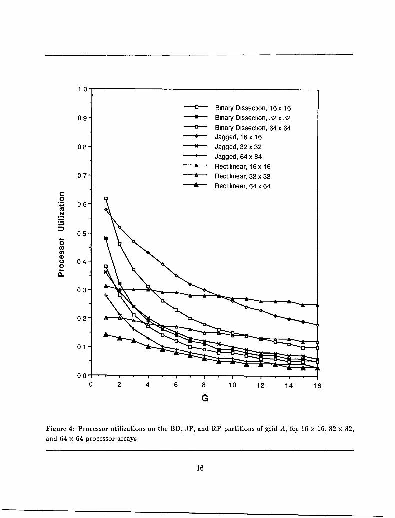
expected, since a rectilinear partition is a constrained version of a binary dissection. Figures 4, 5, and 6, give estimated processor efficiencies on the three grIds, measured as the

estimated speedup divided by the number of processors. Each performance curve is parameterized by G, m order to show how performance is affected by an increasmg cost differential between local

and global communicatIOn. Each graph plots performance curves for each of the three partitioning methods (encoded here as BD,JP,and RP) with 16 x 16, 32 X 32, and 64 x 64 processor arrays. All InItIal RP row partItions were selectmg by computlllg the optImallD partitIOn for N processors.

For grid A we see that BD has a clear advantage over the other methods when global commu­

nIcation is as cheap as local. However, as G grows It lllcreaslllgly suffers from its global edges; On the 16 X 16 and 32 X 32 arrays JP surpasses it once G > 3; however It fails to surpass BD at all on the 64 X 64 array. On a 16 X 16 array, RP sUIpass BD once G 2: 5, and surpasses JP once G 2: 9.

On the 32 X 32 array RP surpass both BD and JP after G 2: 5, whereas on the 64 X 64 array it IS bested by both BD and JP. At thIS extreme point most edges go off processor, and the workload is small. BD's advantage in load balancing then dominates. Observe however that performance at the right end of the curve is not good; this may be indicative of placing too small a problem on the

14

Processor array 16 X 16 32 X 32 64 X 64

(fr, fE, fu) (fr, fE, fu) (fr,fE,fu) Binary Dissection (0.73,0.32,0.98) (0.49,0.29,0.92) (0.19,0.24,0.72) Jagged Partitioning (0.70, 0.79,0.84) (0.45, 0.73,0.68) (0.19,0.52,0 53) Rectilinear Partitioning (0.77,0.91,0.27) (0.61,0.82,0.27) (0.37,0.68,0.24)

fr, fE, and fu values for GrId A

Processor array 16 X 16 32 X 32 64 X 64

(fr, fE, fu) (fr,fE,fu) (fr,fE,fu) Binary Dissection (0.84,0.37,0.98) (0.67,0.37,0.96) (0.37,0.38,0.86) Jagged Partitioning (0.84,0.95,0.98) (0.67,0.87,0.95) (0.39, 0.77,0.86) Rectilinear Partitioning (0.84,0.97,0.92) (0.68,0.94,0.80) (0.44,0.86,0.66)

fr, fE, and fu values for Grid B

Processor array 16 X 16 32 X 32 64 X 64 (fr, fE, fu) (fr, fE, fu) (fr, fE, fu)

Binary Dissection (0.91,0.27,0.99) (0.82,0.29,0.98) (0.62,0.30,0.92) Jagged Partitioning (0 91,0.92,0.98) (0.82, 0.76,0.98) (0.64,0.66,0 92) Rectlhnear Partitiomng (0.91,1.00,0.85) (0.83,1.00,0.85) (0.70,1.00,0.69)

fr, fE, and fu values for Grid C

Table 1: Fraction fr of internal edges, fraction h of external edges which are local, and processor utilizatIOn fu under no communication costs, for dIfferent meshes, processor arrays, and partitioning

methods

machme. GrId B IS much more regular than A, a fact that translates into higher performance under

higher values of G. On the two smaller arrays the RP curves cross the JP and BD curves in the region of G = 5. On the largest array JP is somewhat better than the other methods, whIle the

RP and BD curves are surprisingly similar after G > 3 GrId C was constructed specifically to lughhght RP's advantages over the other methods. Under

RP, none of its edges are global, so performance IS msensltIve to G. RP's cross-over points are again in the region G E (3,5); owing to its complete avoidance of global costs, its performance is substantially better than the others under lugh values of G.

15

1 0

~ Bmary Dissection, 16 x 16

09 • Bmary Dissection, 32 x 32 ~ Bmary Dissection, 64 x 64 0 Jagged, 16 x 16

08 )( Jagged, 32 x 32

Jagged, 64 x 64

* Rectilinear, 16 x 16

07 6 Rectilinear, 32 x 32 .. Rectilinear, 64 x 64 c: 0 - 06 as N

-=» 05

a-0 en en Q) 0 04 0 a-D.

03

02

01

OO~~--~~--r-~-'--~~--~-r~~~~--~~~

o 2 4 6 8 10 12 14 16

G

Figure 4: Processor utilizations on the BD, JP, and RP partitions of grid A, fO.r 16 X 16, 32 X 32,

and 64 X 64 processor arrays

16

~ Binary Dissection, 16 x 16

• Binary Dissection, 32 x 32

1 0 ~ Binary Dissection, 64 x 64 0 Jagged, 16 x 16 M Jagged, 32 x 32

09 Jagged, 64 x 64

* Rectilinear, 16 x 16 6 Rectilinear, 32 x 32

08 • Rectilinear, 64 x 64

07

c 0 - 06 as N -:::::>

05 10..

0 U) U) (1) (.) 04 0 10..

£l.

03

02

01

004-~--~~--r-~~--~~--~-r~--'-~--~~-'

o 2 4 6 8 10 12 14 16

G

FIgure 5: Processor utilizations on the BD, JP, and RP partitions of grid B, for 16 X 16,32 X 32,

and 64 X 64 processor arrays

17

~ Binary Dissection, 16 x 16

• Binary Dissection, 32 x 32 c Binary Dissection, 64 x 64 0 Jagged, 16 x 16

1 0 M Jagged, 32 x 32 Jagged, 64 x 64

* Rectilinear, 16 x 16 09 :6 Rectilinear, 32 x 32

* Rectilinear, 64 x 64

08

07

c 0

06 -tU N

.--::J 05 a-0 VI VI Q)

04 ()

0 a-D..

03

02

01

004-~--~~--r-~~~~~--T--r--~-r~~'-~--;

o 2 4 6 8 10 12 14 16

G

Figure 6: Processor utilizations on the BD, JP, and RP partitions of grid C, for 16 X 16, 32 X 32, and 64 X 64 processor arrays

18

Processor array 16 X 16 32 X 32 64 X 64

Grid A 13 11 37 Grid B 9 11 19 GndC 5 5 5

Table 2: Iterations used by iterative refinement to converge

On these problems, rectilinear partItioning required far fewer iterations to reach convergence than would be suggested by Lemma 5. Table 2 gives the number of iterations required for each of the nine rectilinear partitIOns generated.

We also evaluated the cost of these partitions assummg that diagonally adjacent processors are connected in the local network. In every case the performance of BP was completely unaffected. RP's performance improved slightly, usually by no more than 10%. JP's performance improved sharply, to the extent that it outperforms RP on almost all the Gnd A and Gnd B partitions. RP retains its supenority on Grid C. These results suggest that jagged partitions effectively capture localIty when that locality is defined to include diagonally connected processors. Of course, th~re

IS no guarantee that a jagged partItion will map perfectly onto an 8-neighbor mesh; an interesting future line of inqUIry is to develop algonthms that guarantee such localIty. Rectilmear partitions

are most desIrable when the rectIlinear constraint matches the rectilinear nature of North-East­West-South meshes.

The data presented here indicates that rectilinear partitions have their utIlity. When global communication values are high, It is worthwlule to accept some load Imbalance for the sake of

communication locality. On the other hand, it is clear that rectilinear partItions are not desirable when the problem is hIghly Irregular and global communicatIOn is comparatively cheap. We plan further expellmentatIOn WIth these partitionlllg strategies on actual codes on actual maclunes.

5 Three Dimensional Partitioning

We have already seen that RPP m one dImenSIOn can be solved m polynomIal tIme; It is not yet known whether the two-dImensIOnal problem is tractable. In this section we demonstrate that RPP m three dImensions IS NP-complete. We establIsh the fact by demonstratmg that an arbItrary monotone 3SAT problem [8] can be solved by any three-dImensIOnal RPP algorithm. Since the monotone 3SAT problem is NP-complete, so is RPP in three dImensIOns.

The general 3SAT problem has the following form. We are given n Boolean literals Xl, ... , X n ,

and m clauses CI , ... , Cm. Each clause is the disjunctIOn of three distinct literals, each of which

may be complimented or uncomplImented. For example, (Xl + X3 + X17) and (Xl + X2 + X14) are two clauses. The 3SAT problem is to find a Boolean assignment for each lIteral such that every clause evaluates to true. The monotone 3SAT problem requires that every given clause have either

19

all complimented literals, or all un complimented literals. A useful consequence of the monotone

restriction is that for any given triple of literals (X"X3 ,Xk) there are at most two clauses involving all three sImultaneously-one where they are all complimented, and one where they are not. It

has been shown that the monotone 3SAT problem is NP-complete [8]. Minor modifications to the approach we develop will work for general 3SAT problems; it is simply easier to describe the

transformatIOn if we assume the clauses are monotone. A choice of partitIOnmg can be interpreted as an assignment of Ii teral values and assessment of a

clause's truth value. We first introduce these ideas by application to the monotone 2SAT problem, where clauses have two literals (2SAT can be solved in polynomial time). Let Xl and X2 be two

literals; only two monotone clauses are possible, (Xl + X2) or (Xl + X2)' In either case, only one assignment of values to the literals can cause the clause not to be satisfied, Xl = X2 = 0 in the former case and Xl = X2 = 1 in the latter We capture tlus in a partltiomng framework with a 3 X 3 domain with binary workload weIghts, to be partitIOned into four pieces. The center weIght is 1; one corner is also weighted with 1 dependmg on the clause, and all other weights are O. FIgure 7(a) illustrates the domain, and the assignment of mJeaszbzlzty products XIX2, XIX2, XIX2, and XIX2 to opposing corners. The choice of a row partition corresponds to an assignment to Xl, the chOIce of a column partition corresponds to an assIgnment to X2. Our weighting rule is to assIgn a 1 to a

corner whose mfeasibllity product is true when the correspondmg truth assignment fails to satisfy the clause. Thus, if (Xl + X2) is a problem clause, then the XIX2 corner is given a 1; If (Xl + X2) is a clause then the XIX2 corner is given a 1. If both clauses appear m the problem, both correspondmg corners are weIghted by 1. ThIS is eqUIvalent to requinng that Xl ED X2 = 1 (ED being the exclusIve OR operator). Also, in our problem transformatIOn it WIll be possible for Xl and X2 to represent the same lIteral. If thIS is the case, we place Is m the XIX2 and XIX2 corners, in order to force a common selection for the lIteral, in both Its column and row representatIOns. Figure 7(b) and (c) illustrates the weighting corresponding to conditions (Xl + X2) and (Xl ED X2) respectively, and shows the partition corresponding to the assIgnment Xl = 0, X2 = 1. Observe that the bottleneck weight is 1, whereas It would be 2 If the infeasIble assignment Xl = 0 and X2 = 0 were chosen. The infeasible assignment is the only one achIeving a bottleneck cost of 2. This is true of the construction for any clause, and is the key to detelmmmg whether the aSSIgnment corresponding to some partitioning satisfies all clauses.

A monotone 2SAT plOblem can be transformed into a rectilinear partitionmg problem usmg the

Ideas expressed above. GIven n literals Xl,. ., Xn we will create a (4n -1) X (4n - 1) binary domain. For each variable we assign three contiguous rows, and three contiguous columns. Vanables' sets of rows and columns are separated by a single "paddmg" row and single "padding" column whose

purpose will be to force a partitIOn within each vanable's set of rows, and within each variable's set of columns. We aSSIgn Is and Os described above for the 3 X 3 intersection of Xl'S rows and

X3 's columns. Elements at the intersection of two variables that never appear in the same clause are all assigned value O. We place a 0 wherever a "middle" row for a variable meets a padding column; likewise, we place a 0 wherever a vanable's middle column meets a padding row. OtherwIse, every other entry of a padding row or a paddmg column is 1. The construction for the problem

20

o 1 0

~=1

(a) General construction of domain to represent a clause

0 0 0

0 1 0 1 0 0

~=1

(b) Domain for ~ + ~, partition for assignment

~=O, ~=1

0 0 1

0 1 0 1 0 0

~=1

(c) Domain for ~ e ~

Figure 7: TransformatIOn of 2SAT Problem into Rectilinear Partitioning Problem

(Xl + X2)(X2 + X3) is shown in Figure 8. We seek an optimal rectilinear partitioning of this domain onto a (3n - 1) X (3n - 1) array of processors. Weights in padding rows and columns are defined in such a way that for a bottleneck weight of 1 to be achieved it is necessary that a partition never

group padding and non-padding rows or group padding and non-padding columns. This forces a partition of every varIable's rows, and every variable's columns.

If the domain can be partitioned and achieve a bottleneck cost of 1, then the 2SAT problem is solved by the assignment implicit in the optimal partitioning. Otherwise the 2SAT problem cannot

be solved. Figure 8 also illustrates the partition corresponding to the solution Xl = 1, X2 = 0, and

X3 = 0 The extension of these constructs to three dimensIOns is straightforward. Let XI, X2, X3 be

literals. In a monotone 3SAT problem the only possible clauses are (Xl +X2 +X3) and (Xl +X2 +X3);

III the former case only the assignment Xl = X2 = X3 = 0 falls to satisfy the clause, in the latter case only Xl = X2 = X3 = 1 fails to satisfy the clause. In the event that both clauses appear, theIr conjunction is not satisfied If and only if the variables are all assigned the same value Now let us associate a 3 X 3 X 3 clause regzon with these literals. The 2SAT constructIOn associated Xl with the Y dimension and X2 with the X dimension; we augment this and associate X3 with the Z dimension. It is convenient to view a clause region as three stacked 3 X 3 arrays with XY orientation. The

centermost element of the middle array will have value 1, all other elements of the middle array are O. Like the 2SAT problem, the four corners of the lowest 3 X 3 array represent products of all

three literals. In the 3SAT case, all products in the "bottom" array include X3 and all products III

21

, , , I I

0 10 0 .1_0.12- 1 .!2LO_L 1 -0- ~. ~-~--o 110 011 0 011 0

0 011 1 0 10 0 1 010 0 I I •

1 011 1 1io 1 1 1io 1

0 01

1 1 1 10 0 1 0 10 0 I I I o 110 0 011 0 0 ~.QL1_<L_ "0-010' ~- "OTO-1 --I 1 010 0

forced by paddmg

I I I

1 01 1 1 110 1 1 1io 1 LIteral value selectIon ------_. 0 0 10 1 0 10 0 1 110 0 I I I o 110 0 011 0 0 . .Q11_~_

0-0'0 ~1- "Oro-a -1- 010 1 I I I

Figure 8: Example of 2SAT problem (Xl + X2)(X2 + X3) mapped to 2D rectilinear partItIOmng of 9 X 9 bmary domain onto 6 X 6 array of processors. Partition of solution Xl = 1, X2 = 0, X3 = 0 is

shown

the "top" array include X3. The Xl and X2 combinatIOns are identIcal to the 2SAT problem. For

example, the infeasibility products in the northwest, northeast, southwest, and southeast corners

of the top array are X-IX2X3, X-IX2X3, XIX2X3, and XIX2X3 respectIvely. LIke the 2SAT problem, we

weight a corner wIth 1 if the truth assignment satisfying the correspondmg infeaSIbIlIty product

faIls to satisfy the clause. Thus, if (Xl + X2 + X3) appears as a clause, we place a 1 in the Xl X2X3

corner. If (Xl + X2 + X3) is a clause then we place aIm the XIX2X3 corner. Both Is are placed If both of these clauses appear m the problem. All other entries of the clause region are O. All clause

regions corresponding to three distinct literals that do not appear m a clause are zeroed out. Clause regions involving intersections of a literal and itself are weighted to ensure that a bottleneck value

of 1 is achieved only if partitions are chosen corresponding to the same selection of literal value in

each dimension. For example, if Xl and X3 happen to be the same literal, then a 1 is placed many

corner whose product involves XIX3 or XIX3.

ASSIgnment of a value for Xl corresponds to selection of a plane with Y Z orientation. The

22

plane'S intersection wIth each layer in the clause region looks the same-it is either the Xl = 0

line or the Xl = 1 line as seen in the 2SAT problem (Figure 7). Similarly, assignment of a value for X2 corresponds to a plane whose intersection with each layer is identical, eIther the line for

X2 = 0 or the lme for X2 = 1. Finally, selection of X3 = lIS accomplished by selecting an XY plane that separates the bottom two layers from the top layer, wIllIe selectIOn of X3 = 0 separates the bottom layer from the top two. Under this construction, selection of planes corresponding to an assignment that makes an infeasibility product true will place the centermost 1 in the same volume as the "infeasibility 1", giving rise to a bottleneck weight of 2. This fact is important enough to state formally.

Lemma 6 Let I( XI, X2, X3) be any mJeaszbzlzty product whose posztzon m a clause regzon zs set to

value 1. Then any partztzon whose assoczated assignment sets I( X}, X2, X3) = 1 places the mJeasz­

bzlzty 1, and the clause regzon's center 1 m the same partztzon volume. The bottleneck cost oj any

such partztzon IS a~ least 2.

Like the 2SAT mapping, we add "padding" layers to ensure that any partition with cost 1 must choose one of two planes in each dimension of each clause region. The assignment of Is and Os to paddmg layers is similar to the 2SAT case. Figure 9 defines the assignment in terms of how each layer's elements are weighted in the immediate vicmity of a clause region. Figure 9(a) shows how a portIOn of the padding layer with (XY orientation) is weighted when centered directly above or below a clause region (the heavy lines illustrate how the clause region is positioned). The only way to separate the three Is in each corner is to choose the four partitioning layers with XZ orientation and four with YZ orientation that do not intersect the 3 X 3 core. These layers ensure that no elements on the XZ and YZ faces of the clause region WIll be grouped with any elements from any other clause region-at least if a bottleneck cost of 1 is to be achieved. Figures 9(b) and (c) then show how to weight elements in padding layers with XZ and YZ orientation, depending on whether the padding layer intersects a layer containing a boundary or middle layer of the clause

region. Weights for the clause region (which is outlined) are not included. The corner Is seen in Figure 9(b) are adjacent to the corner Is seen in Figure 9( a)j in order to achieve a bottleneck cost

of 1 it will be place two partitIOning planes with XY orientation to contain the XY padding layer. This ensures that any element at an XY face of the clause region will not be grouped with elements

from any other clause region. To transform a monotone 3SAT problem we construct a (4n - 1) x (4n - 1) X (4n - 1) domain

The first three coordmate positions in each dImensIOn correspond to Xl j the fourth coordinate position m each dimension corresponds to padding, the next three coordinate positions m each dimenSIOn correspond to X2, and so on. The domain is weighted as described above. We have seen that in order to achieve a bottleneck cost of 1 it is necessary to contain each padding layer with

two partitlOnmg planes. ThIS defines (2n - 1) planes orthogonal to each dimension. Furthermore, It is also necessary to appropriately partItion each clause regIOn in each dImension. This leads to

an additional n partitioning planes orthogonal to each dimension. Consequently, the dimensions of the target architecture are (3n - 1) x (3n - 1) X (3n - 1).

23

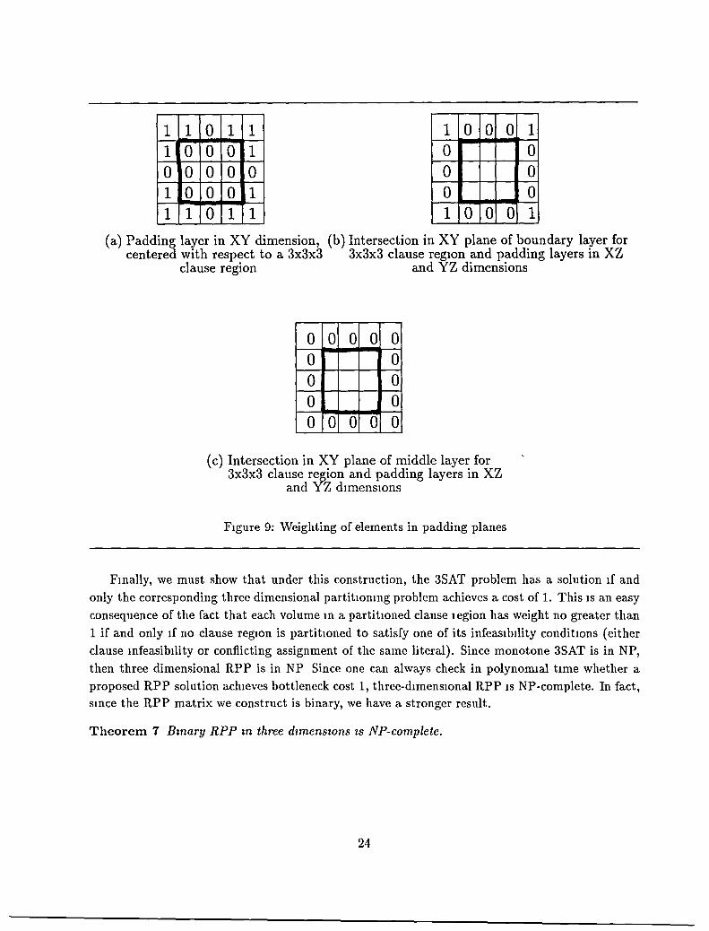
1 1 0 1 1 1 0 0 0 1 1 I 0 0 0 1 0 0 0 0 0 0 0 0 0 1 0 0 0 1 0 0 1 1 0 1 1 1 0 o 0 1

(a) Padding layer in XY dimension, (b) Intersection in XY plane of boundary layer for centered with respect to a 3x3x3 3x3x3 clause regIOn and padding layers in XZ

clause region and YZ dimensions

0 o 0 0 0 0 0 0 0 0 0 0 o 0 0 0

( c) Intersection in XY plane of middle layer for 3x3x3 clause region and padding layers in XZ

and YZ dImensIOns

FIgure 9: Weighting of elements in padding planes

Fmally, we must show that under this construction, the 3SAT problem has a solution If and

only the corresponding three dimensional partitIOnlllg problem achieves a cost of 1. This IS an easy consequence of the fact that each volume III a partitIOned clause legion has weight no greater than

1 if and only If no clause regIOn is partitIOned to satisfy one of its infeasIbility conditIOns (either clause lllfeasibility or conflicting assignment of the same literal). Since monotone 3SAT is in NP, then three dimensional RPP is in NP Since one can always check in polynomIal tIme whether a proposed RPP solution aclueves bottleneck cost 1, three-dImensIOnal RPP IS NP-complete. In fact, Slllce the RPP matrix we construct is binary, we have a stronger result.

Theorem 7 Bmary RPP m three dzmenszons zs NP-complete.

24

6 Summary

ThIS paper examines the problem of partitioning with one, two, or three dimensional rectilInear partitions. When used to balance workload in data parallel computatIOns having localized commu­

nication, such partitions can be expected to reduce the need for expensive global communication. For the one-dimensional case we improved upon the best published solution to date when

m ~ M, reducing the cost of finding the optimal partition of m modules among M processors to Oem + (Mlogm)2). For the two-dimensional case we showed how it is possible to find the best possible partitioning in a given dimension, provided that the partition in the alternate dimension remains fixed. This result can be used to find the optimal partition in two dimensions, but with

exponentially large cost (if the numbers of processors In both dimensions is a problem parameter). The result also serves as the basis for a heuristic that iteratively improves upon a solutIOn. The heuristic is shown to converge to a fixed point, in a bounded number of iterations. Empirical studies show that the heuristic may provide some performance advantage when the differentIal between

the local and global network bandWIdth is moderately large. FInally, we showed that the problem of finding an optimal three dimensional rectilinear partition is NP-complete.

Acknowledgements

We thank Adam Rifkin for his help in programming. DiSCUSSIOns on this problem with Joel Saltz and Shahid Bokhari were, as always, quite useful.

References

[1] M.J. Berger and S. H. Bokhari. A partitIOnIng strategy for nonuniform problems on multipro­cessors. IEEE Trans. on Computers, C-36(5)·570-580, May 1987.

[2] F. Berman and L. Snyder. On mappIng parallel algOrIthms Into parallel architectures Journal

of Parallel and Dzstrzbuted Computzng, 4:439-458, 1987.

[3] S. H. Bokhari. PartitIOnIng problems in parallel, pIpelined, and distributed computing. IEEE Trans. on Computers, 37(1):48-57, January 1988.

[4] M.Y. Chan and F.Y.L Chin. On embedding rectangular grids in hypercubes. IEEE Trans.

on Computers, 37(10):1285-1288, October 1988.

[5] H.-A. Choi and B. NaraharI. Algorithms for mapping and partItioning chain structured parallel computations. In Proceedmgs of the 1991 Int'l Conference on Parallel Processmg, St. Charles, illinois, August 1991. To appear.

[6] F. Ercal, J. Ramanujam, and P. Sadayappan. Task allocation onto a hyercube by recurSIve mincut partitioning. Journal of Parallel and Dzstrzbuted Computmg, 10:35-44, 1990.

25

[7] G. Fox, A Kolawa, and R. WIlhams. The implementatIOn of a dynamic load balancer. Tech­

nical Report C3P-287a, Caltech Report, February 1987.

[8] M.R. Garey and D.S. Johnson. Computers and Intractabzlzty. W.H. Freeman and Co., New

York, 1979.

[9] C.-T. Ho and S.L. Johnsson. On the embedding of arbitrary meshes In boolean cubes with expansion two dilation two. In Proceedmgs of the 1987 Int'l Conference on Parallel Processmg,

pages 188-191, August 1987.

[10] O.H. Ibarra and S.M. Sohn. On mapping systolic algorithms onto the hypercube. IEEE Trans.

on Parallel and Dzstrzbuted Systems, 1(1):48-63, January 1990.

[11] M.A. Iqbal. Approximate algorithms for partItioning and assignment problems. Technical

Report 86-40, ICASE, June 1986.

[12] M.A. Iqbal and S H. BokhaIi Efficient algorIthms for a class of partitionIng problems. Tech­nical Report 90-49, ICASE, July 1990

[13] R. Kincaid, D.M. Nicol, D. Shier, and D. RIchards. A multistage linear array assignment problem. Operatzons Research, 38(6).993-1005, 1990

[14] C.-T. King, W.-H. Chou, and L.M. Ni. Pipelined data-parallel algorithms. IEEE Trans. on

Parallel and Dzstrzbuted Systems, 1(4):470-499, October 1990.

[15] D.J. Mavnplis. Multigrid solution of the two-dimensional Euler equations on unstructured trIangular meshes AIAA Journal, 26:824-831, 1988.

[16] R G. Melhem and G.-Y. Hwang. Embedding rectangular grids into square grids with dIlation two. IEEE Trans. on Computers, 39(12):1446-1455, Decemeber 1990.

[17] D.M. Nicol and D.R. O'HallalOn. Improved algorIthms for mapping parallel and pipelined computations. IEEE Trans. on Computers, 40(3):295-306, 1991.

[18] D. A Reed, L. M. Adams, and M. L. Patrick. Stencils and problem partitionings: Their influence on the performance of multIple processor systems. IEEE Trans. on Computers,

C-36(7):845-858, July 1987.

[19] P. Sadayappan and F. Ercal Nearest-neighbor mapping offimte element graphs' onto processor meshes. IEEE Trans. on Computers, 36(12):1408-1424, December 1987.

[20] J. Saltz, S. Petiton, H Berryman, and A. Rifkin. Performance effects of irregular commu­nicatIOn patterns on massively parallel multiprocessors. Journal of Parallel and Dzstrzbuted

Computmg, 1991. To appear. Available as ICASE Report 91-12, ICASE, NASA Langley Re­search Center, MS 132C, Hampton, VA 23665.

26

[21] D.S. Scott and R. Brandenburg. Minimal mesh embeddmgs in binary hypercubes. IEEE Trans.

on Computers, 37(10):1284-1285, October 1988.

[22] L W. Tucker and G.G. Robertson Architecture and applIcations of the Connection Machine Computer, 21 26-38, August 1988.

[23] S. VavasIs. Automatic domain partitioning m three dImensIOns. SIAM Journal on Sczentzjic and Statzszcal Computmg, July 1991. To appear.

[24] D.L. Whitaker, D.C. Slack, and R.W. Walters. Solution algorithms for the two-dimensional Euler equatIOns on unstructured meshes. In Proceedmgs AIAA 28th Aerospace Sczences Meet­mg, Reno, Nevada, January 1990.

27

! I\U\SI\ Report Documentation Page ..... 10'\) o...er""'.aulC(.rI"\.~ , ¥"~ <)" '-'ST alif

I 1 Report No 2 Government Accession No 3 RecIpient's Catalog No NASA CR-187601 ICASE Report No. 91-55

4 Title and Subtitle 5 Report Date

RECTILINEAR PARTITIONING OF IRREGULAR DATA July 1991 PARALLEL COMPUTATIONS

6 Performing Organization Code

7 Author(sl 8 Performing Organization Report No

Davl.d M. Nicol 91-55

10 Work Unit No

9 Performing Organization Name and Address 505-90-52-01

Instl.tute for Computer Applicatl.ons l.n SCl.ence 11 Contract or Grant No

and Engl.neering NASl-18605 Mal.l Stop l32C, NASA Langley Research Center

Hampton, VA 23665-5225 13 Type of Report and Period Covered

12 Sponsoring Agency Name and Address Contractor Report Natl.onal Aeronautl.CS and Space Adminl.stratl.on

Langley Research Center 14 Sponsoring Agency Code

Hampton, VA 23665-5225

15 Supplementary Notes

Langley Technical Monitor: Subml.tted to Journal of Parallel Ml.chael F. Card and Distributed Computl.ng

16 Abstract

Thl.s paper descrl.bes new mapping algorl.thms for domal.n-orl.ented data-parallel computations, where the workload is dl.stributed irregularly throughout the domain, but exhl.bl.ts locall.zed communl.catl.on patterns. We consider the problem of parti-tl.Oning the domal.n for parallel processing in such a way that the workload on the most heavl.ly loaded processor is miniml.zed, subJect to the constraint that the partl.tl.on be perfectly rectl.ll.near. Rectilinear partl.tl.ons are useful on archl.-tectures that have a fast local mesh network and a relatively slower global net-work; these partl.tions heurl.stically attempt to maxl.mize the fraction of communica-tl.on carrl.ed by the local network. Thl.S paper provl.des an improved algorithm for findl.ng the optimal partl.tion l.n one dl.mensl.on, new algorithms for partl.tl.oning in two dl.mensl.ons, and shows that optimal partl.tl.onl.ng l.n three dl.mensl.ons l.S NP-com-plete. We dl.sCUSS our appll.catl.on of these algorl.thms to real problems.

17 Key Words (Suggested by Author(sll 18 Distribution Statement

mappl.ng, partl.tl.onl.ng, rectl.ll.near, 61 - Computer Programml.ng and Software algorl.thms

Unc1assl.hed - Jlnl l.ml. ted 19 Security Classl! (of thiS report I 120 Security Classlf (of thiS pagel 21 No of pages 22 Price

Unclassl.fl.ed Unclassifl.ed 29 A03 , NASA FORM 1626 OCT at

NASA-Langley, 1991

End of Document