Embed Size (px)
Citation preview

Artificial Intelligence 78 (1995) 179-212
Artificial Intelligence
ELSEVIER
Learning to track the visual motion of contours
Andrew Blake *, Michael Isard, David Reynard Department of Engineering Science, University of Oxford, Parks Road, Oxford OX1 3PJ, UK
Received June 1994: revised December 1994
Abstract
A development of a method for tracking visual contours is described. Given an “untrained” tracker, a training motion of an object can be observed over some extended time and stored as an image sequence. The image sequence is used to learn parameters in a stochastic differential equation model. These are used, in turn, to build a tracker whose predictor imitates the motion in the training set. Tests show that the resulting trackers can be markedly tuned to desired curve shapes and classes of motions.
1. Introduction
A significant recent development in real-time visual sensing has been the invention
of contour trackers [25] that can track the motion of silhouettes and surface features. This allows the camera to be treated as a sparse sensor with consequent processing efficiency that lends itself to real-time operation. There are many potential applications, for instance in biomedical image analysis (e.g. [ 31) , in surveillance (e.g. [23,31,33] ), in autonomous vehicle navigation (e.g. [ 171) and in hand-eye coordination for robots [ lo]. A review of existing methods in curve tracking can be found in [ 131.
Real-time video tracking has been achieved for line-drawings [22] and polyhedral structures [ 271 and for simple, natural features such as road edges [ 171. Commercial
systems (e.g. Watsmart, Oxford Metrics) are available which track artificial markers on live video. Natural point features (e.g. on a face) but not curves have been tracked at 10 Hz using a workstation assisted by image processing hardware [ 41. Curve trackers [ 12,16,25] have been demonstrated on modest workstations with some success.
Several researchers have described Kalman filter formalisms for tracking of curves and surfaces [ 34,351. This paper is based on a particular linear filter for curves which
* Corresponding author. E-mail: [email protected].
0004-3702/95/$09.50 @ 1995 Elsevier Science B.V. All rights reserved SSDIOOO4-3702(95)00032-l

180 A. Blake et ul. /Artificial Intelligence 78 (1995) 179-212
incorporates a mean shape-a “template”, as used by a number of researchers [9, 19,21,38]. The tracker used here [ 11,121 also has an afline invariance mechanism
to accommodate 3D rigid transformations of planar shapes. We refer to this as the “untrained” tracker, not yet tuned for motion.
Tuning for specific motions, it transpires, is a key ingredient in achieving robust tracking. It can be done consistently in the Kalman filter framework by defining dynamics within an appropriate state space. Deterministic models of visual motion based on oscillatory modes have been used previously [29]. The generality of motion models
is greatly increased by including a stochastic component in the dynamics, as is done commonly in control theory via stochastic differential equations [ 11. Even in the case of planar rigid motion, the dynamics of a visual contour are potentially complex with six independent modes and many degrees of freedom for the driving noise process.
Therefore, rather than programming ad hoc dynamics, we have developed a procedure to learn them from extended motion sequences. The procedure will be explained and its
effectiveness in tuning a tracker to characteristic classes of motions will be demonstrated. The disadvantage of the method is that each tuned tracker is effective only for the relatively narrow class of shapes and motions on which it was trained. The advantage is that performance is enhanced compared with an untrained tracker, particularly in the ability to ignore background distracters and to follow rapid motions.
2. Tracking framework
The tracker consists of an estimator for a piecewise smooth image plane curve in motion
r(s,t) = (x(s.t),y(s.r)).
Following the tracking formulations of others [ 14,281, the curve representation is in terms of B-splines. Splines of order d are used, with the possibility of multiple knots for vertices. In our experiments, splines are usually quadratic (d = 3). The tracking framework described here follows an earlier one [ 121 but is generalised to allow any learned motion model to be used in the prediction phase of tracking.
2.1. Curve representation
Curves are represented as parametric B-splines with N spans and NC control points.
x(s,r) = B(s)X(t), y(s,t) = B(s)Y(t), O<S<N,
where X = (XI, . . . , XN~ )“ and similarly for Y. The elements of X and Y are simply the x- and y-coordinates of the set of control points (X,, Y,,) for the B-spline. The number of control points is equal to the number of spans (N, = N) for closed curves, whereas NC = N + d for open curves (with appropriate variations, in each case, where multiple knots are used to vary curve continuity). The vector B(s) consists of blending coefficients defined by
A. Blake et al. /Artificial Intelligence 78 (1995) 179-212 181
B(s) = (h(s), . . . ,BN,(S)),
where B,(s) is a B-spline basis function [ 7,181 appropriate to the order of the curve and its set of knots.
2.2. Tracking as estimation over time
The tracking problem is to estimate the motion of some curve-in examples in this paper it will be the outline of a hand or of lips. The underlying curve-the physical truth-is assumed to be describable as a B-spline of a certain predefined form with control points X(t) and Y(t) varying over time. The tracker generates estimates of those control points, denoted k(t) and Y(t) and the aim is that the estimates should represent a curve that, at each time step, matches the underlying curve as closely as possible. The tracker is based, in accordance with standard practice in temporal filtering [ 6,201, on two models: a system model and a measurement model. These will be spelt out in detail later. Broadly, the measurement model specifies the positions along the
curve at which measurements are made and how reliable they are. The system model specifies the likely dynamics of the curve over time, relative to a “template” [ 191 whose control points, (x, y) , are generated by interactive software, used to draw spline curves over a single image captured from live video.
2.3. Rigid body transformations
A tracker could conceivably be designed to allow arbitrary variations in control point positions over time. This would allow maximum flexibility in deforming to accommodate moving shapes. However, particularly for complex shapes requiring many control points
to describe them, this is known to lead to instability in tracking [ 121. It occurs when features are temporarily obscured and the tracker is bumped out of its steady state. The more complex the shape to be tracked, the worse is its instability when lock is lost, and
this is illustrated in Fig. 1. Fortunately, it is not necessary to allow so much freedom. A moving hand, for
instance, provided the fingers are not flexing, is a rigid, approximately planar shape. Provided perspective effects are not too strong, a good approximation to the curve shape as it changes over time can therefore be obtained by specifying Q. a linear vector-valued function of the B-spline coordinates (X, Y) . The Q-parameterisation of the curve embodies the reduced degrees of freedom for motion, which vary online, leaving intact the full set (X, Y) of geometrical parameters to do justice to the detail of complex shapes and to be varied offline only.
The relationships Q H (X, Y) between parameterisations are expressed in terms of two matrices M and W:
(;) =WQ+ (;) Q=M[(;) - (;)I. --
The matrices M and W are defined in terms of the shape template (X, Y). It is known that for a planar shape, for instance, just six afine degrees of freedom are
182 A. Blake ef al./Art~~cial Intelligence 78 (1995) 179-212
Fig. I. Tracking can become unstable when the tracked outline is geometrically complex. This problem can
be overcome, however, by introducing certain constraints into the configuration space of the tracker-see text.
required [26,37] to describe the possible shapes of the curve and this is illustrated in Fig. 2. The space of possible Q-vectors is expressible as a six-dimensional linear subspace of Q-vectors, and a basis for this subspace is:
where the NC-vectors 0 and 1 are defined by:
o= (0,O ,..., O)T, 1= (I. I ,..., I)“.

A. Blake et al./Artijcial Intelligence 78 (1995) 179-212 183
i& (.p& 6 ‘..
f.. f ‘...
..*’ a... ..z ‘*..
. . . . 1. . . . . . . . . . . f.. . . . .
. . . . . . . . . . . . ** .*. . . . . . . . . . . . 8.
Fig. 2. The six degrees of freedom of a 2D affine transformation are illustrated here: translation vertically and horizontally, rotation and scaling vertically, horizontally and diagonally.
In that case, the matrices M and W converting B-spline control points (X and Y) to and from the six-vector Q can be defined, in terms of the template, as follows:
w= 10 x 0 0 ( Y 01orxo > (1)
M= (wTtiw>--IwT~, (2)
where
N
Ii= I( > :, ; 8 UWTBWds, 0
in which @ denotes the “Kronecker product” of two matrices. ’ Note that 3-t is the “metric” matrix that arises from the “normal equations” [ 301 for the problem of least- squares approximation with B-splines. Examples of such matrices are given in [ 121.
Shape models other than planar-affine can be treated by using an appropriate Q-vector of length NQ with a W-matrix of size 2N, x NQ. In the planar-aBine case above we had NQ = 6. Restricted affine motion would call for NQ < 6, for instance rigid 2D
I The Kronecker product A @ B of two matrices A and B is obtained by replacing each element a of A with the submatrix aB. The dimensions of this matrix are thus products of the corresponding dimensions of A and B.

184 A. Blake et al. /Artificial Intelligence 78 (1995) 179-212
Transformations generated by: Dimension No. views
Planar translation X, Y translation 2 I
Planar similarity +X, Y rotation, scaling 4 I
Planar-afine 3D Euclidean, planar curve 6 I
3D affine 3D Euclidean, space curve 8 2 (3)
3D affine+ 3D Euclidean, silhouette 11 3 (6)
Constrained non-rigid + linear deformations fn fn (key frames)
Unconstrained non-rigid B-spline configurations 2N,
Fig, 3. Configuration subspaces-hierarchy for increasing complexity of object and motion.
translation for which NQ = 2. Non-planar rigid shapes can be treated in a similar way to planar ones except that then NQ = 8. For smooth silhouette curves, it can be shown that NQ = 11 is appropriate.’ Finally, non-rigid motion can be treated in the same framework. In each case, the M-matrix continues to be derived from the W-matrix via the formula (2) above. The table in Fig. 3 summarises the hierarchy of models.
Given the compact representation of a curve in terms of configuration-space vector Q, the parametric B-spline can be fully reconstructed from it. The reconstruction formula
is:
r(s,t) = ucs)Q(t), (3)
where
2.4. Curves in motion
Now a state vector can be chosen according to the order of the differential equation
that will describe the motion. Here second-order motion is assumed so the state X is defined in the following form:
x=
The dynamics of the object are then defined by the stochastic differential equation
2=F(X-X)+ G”w ( ( 1 where F is a ~NQ x ~NQ matrix defining the deterministic part of the dynamics. Its eigenvectors represent modes of oscillatory motion, and the corresponding eigenvalues
* In the case of silhouettes, however, the Q-vector representation of the curve is an approximation, valid for
sufficiently small changes of viewpoint.

A. Blake el al. /Art@cial Intelligence 78 (1995) 179-212 18.5
give natural frequencies and damping constants for those modes [ 21. The random part of the dynamics is modelled by a driving noise source w(t) which is a unit NQ- dimensional Wiener process-Brownian motion in continuous time [ 1 ] defined by its statistical properties:
E[w(t)l = 0, E[w(t)w(tjq = tzfQ*
(I, denotes the r x r identity matrix.) The form of the noise process corresponds to the modelling assumption that random processes enter the system only as accelerations,
with no direct coupling to velocities. The covariance coefficient of random acceleration is then GGT and is the observable part of G that, in principle, can be estimated by a learning algorithm. The mean state x of the contour incorporates a mean positional displacement (relative to the template), and a mean velocity which may be taken to be zero or could, in principle, be learned from data.
2.5. Discrete-time model
It is natural to model the motion of an object in continuous time, as we have so far. Discrete time enters only when the measurement process is considered. In the case of video imagery, measurements are made synchronously at a sample interval A.
In between sampling epochs, the continuous equations of motion (5) can be integrated [ 201 to give X,+1 c X( (n+ 1) A) in terms of A’,, E K( nd). Note that no approximation
is introduced here in integrating the continuous dynamics; the discrete representation is
simply a restriction of the continuous one to the sampling epochs. The discrete model has the form
X n+,-x=A(Kn-X)+ .
The matrix coefficient A is a ~NQ x ~NQ matrix, defining the deterministic part of the
dynamics. Its eigenvectors represent modes, as before, in the continuous case. In fact the discrete dynamics matrix A is simply related to the continuous one by
A = exp FA, (7)
so that for an eigenvalue A of A, there is a corresponding (complex) eigenvalue of F,
from which frequency w and damping constant p can be computed:
-p+iw= ilogh. (8)
Without loss of generality, A can be standardised to the form
A= (9)
so that x must be now of the form
e x= - ( > Q

186 A. Blake et al. /Artificial Intelligence 7R (1995) 179-212
depending on mean position in the form of the displacement e but not on mean velocities (which now, in the discrete case, are carried by the A-matrix).
In that case, the equations of motion are simplified to the standard form:
Q ,1+2=A~Qr,+A~Q,,+,+(l -‘Ao-Adi?+&. (10)
As for the stochastic component of the discrete dynamics, at each time YZ, the w, are
independent vectors of independent unit normal random variables. This noise process is then transformed by the matrix B which couples the driving noise into the various natural modes of the deterministic dynamics. In fact B is not completely observable, only the
covariance C = BBT can be computed; this is because the probability distribution for w, being a vector of i.i.d. normal variables, is (it is easily shown) invariant to orthogonal transformations of w.
2.6. Measurement model
In an earlier framework [ 121, measurement was represented as a continuous time process, not because this is a realistic model-after all, video is a synchronous sampled data stream-but because it is tractable in the sense of facilitating analysis of the
tracker’s performance as a control system. Here however, the learned motion models are too varied to allow the kind of performance analysis that was possible for constant velocity models. Therefore, in this paper, a synchronous, discrete-time measurement model is used throughout.
Given an estimator (see next section) i( S, t) for the contour r(s, t), the visual measurement process at time I consists of casting rays along normals fi(s, t) to the
estimated curve and, simultaneously at certain points s along the curve, measuring the relative position ~(5, t) of a feature (typically a high contrast edge) along the ray, so
that
v(.s,t) = [r(s,t) - f(s,t) J . A(s,r) + L’(S,f), (11)
where u( S, t) is a scalar noise variable, assumed gaussian, with a variance a* that will be taken to be constant, both spatially and temporally. Defining measurement to be along the normal only is essential as displacement tangential to the curve is unobservable, the well-known “aperture problem” of visual motion [ 241.
Each measurement v is actually an “innovation” measure [ 61 because it is taken rela- tive to the estimated position i( s, t). This is convenient for tracking because innovation
is a form of error signal, ready to be added in, via an appropriate gain, to the estimated state. In order to compute this gain, we need first to express v in terms of the state vector X, by means of a measurement matrix H(s) :
~(~,t)=H(s,t)(~-X)+I’(S,~). (12)
where, from (3), (4) and (1 I).
H(s,t) = (ii(.~,r)~@B(~) 0)W (13)

A. Blake et al. IArtijicial Intelligence 78 (I 995) 179-212 187
3. Tracking algorithms
3.1. Full time-varying jilter
Following standard practice in filtering, the estimator i%?(t) in state space evolves
in two phases [20]: prediction and measurement. For each phase there is a first-order (mean) and second-order (covariance) update equation.
The prediction phase is applied once at each time step (t - A) + t. The first- and
second-order update equations are respectively the mean and variance from a simulation of the system dynamics (6) :
& = A/i,_l + (I - A)X,
0 0
P,=AP,,_,AT+
i I7 0 c
(14)
(15)
where P, is the covariance of the estimate 2 at time t = nA. In general, the evolution
of P over time has been found to be valuable for contour tracking both in exploiting continuity of motion via the time-varying Kalman gain (see below), and in recovering from sensing failures using a validation gate [ 121.
Following the prediction step for a given time step (t - A) + t, a number of measurements can be made, taken by casting normals on the image field or frame for that epoch. For each measurement, the curve estimate is updated as follows:
& + & + Kv,
where V(S) is innovation along the curve normal at s as before. The Kalman gain for
that measurement [20] is
K=P,HT(HP,HT++‘.
After the measurement has been applied via the Kalman gain to the estimated state zN,. its covariance must be updated:
P,, -+ (I - KH)P,,.
3.2. Steady-state jilter
For many of the experiments reported in this paper we maintain steady-state Kalman gains for each measurement in a fixed sequence of measurements. This is efficient because the computational cost of recomputing P is avoided, and in practice allows more complex spline curves within the constraint of full field-rate (50Hz) tracking. Of course the benefits of variable gain are lost and practically this limits the recovery performance of the tracker after lock is lost, as the last experiment of the paper shows. The steady-state tracker is the restriction of the full tracker (assuming a stable system) to the case that

188 A. Blake et al. /Artificial Intelligence 78 (1995) 179-212
( 1) the sequence of curve positions s at which measurements are made is fixed from iteration to iteration,
(2) the contour is fully locked, (3) all transients in the filter have settled out, (4) curve normals do not rotate-in practice we require deviations from 2D transla-
tional motion to be small. Steady-state gains for the measurement sequence are computed by allowing the filter to run fully locked for a few seconds-it is typically most convenient to do this simply
by leaving the tracked object in its starting position, against a plain background-then freezing the gains, one gain for each curve normal in the fixed measurement sequence.
3.3. Bootstrapping
In order to collect a training set, some form of untrained tracker is required. Since
the dynamics of the moving object are unknown at this stage it is necessary to use a tracker with reasonable default dynamics. Such a tracker is less powerful than a trained
tracker, particularly in clutter and with rapid motions, as this paper will show. To make up for that loss of performance, the training set can be gathered from gentle motion against an uncluttered background. To learn rapid motions, it is necessary to bootstrap, that is: first use a default tracker to learn a relatively slow motion, then incorporate that learned motion into a tracker which should then be more agile than the default, and use it to learn a somewhat faster motion, and so on, repeating the cycle as necessary.
The default trackers are based on constant velocity translational dynamics, with a
damped elastic coupling of shape parameters to those of the template. The stochastic component of the dynamics is a homogeneous, isotropically distributed random acceler- ation, as described previously in some detail [ 121. The deterministic component of the object dynamics for a usable default tracker is given by:
0 I
F= (16) -(w*E + d*E') -2(PE + /?‘E’)
where E’ is a projection matrix onto a certain privileged subspace of curve motions and E projects on the remainder of the state space left when the image of E’ and the subspace of rigid translations are removed. Therefore I - E - E’ is a matrix that
projects the state Q onto the subspace of rigid translations, and EE’ = 0. For example, E’ could be a projection onto the space of rotations/expansions of the template. This would allow unconstrained, constant-velocity translation and also independent control over the strength of the template both for rotation/expansion (via p, w) and for other deformations of shape (via p’, CO’). Further elastic damping parameters can be added to control translational motion, if desired, but we have found, in practice, that it is usually satisfactory to leave translational motion unconstrained.
In the discrete implementation, there is a limit to how large an effective value of the /?, /3’ parameters can be achieved [ 21. However it is, of course, possible to achieve “hard’ settings in which /?, w or /?‘, U’ are effectively infinite, simply by using a smaller

A. Blake et al./Art@cial Inrelligence 78 (1995) 179-212 189
Q-space that excludes the degrees of freedom that are to be set “hard”. This reduced space is specified by removing columns of the W-matrix in ( 1) corresponding to those degrees of freedom.
In later learning experiments reported in this paper, both default and trained trackers are full Kalman filters with time-varying gains and spatially distributed validation gate.
Earlier experiments used steady-state trackers obtained by allowing the full filter to settle down under conditions of full feature-lock. The steady-state gains for the default tracker could, in principle, have been obtained in the same way; instead we use something a little simpler, a form of CY - p tracker [ 201.
4. System identification
The learning task is now to estimate the coefficients Ao, AI and B from a training
sequence Q,,..., Q,, gathered at the image sampling frequency of l/A = 50 Hz. As
mentioned earlier, it is impossible in principle to estimate B uniquely, but the covariance coefficient C = BBT can be determined, from which a standard form for B can be
computed as:
B=fi, (17)
applying the square root operation for a positive-definite square matrix [ 51. The learning process is outlined below. First, to avoid overfitting, the state space
must be restricted, during learning, to a low-dimensional subspace. This could be the six-dimensional “affine” subspace of the state space or some other space spanning an appropriate combination of rigid and non-rigid degrees of freedom. Secondly, Maximum
Likelihood Estimation (MLE) is implemented via least-squares minimisation to obtain discrete-time system parameters. The result is a tracker tuned to those affine motions
that occurred in the training set.
4.1. Estimation for one-dimensional variation
First the estimation algorithm is described for the simple case of a one-dimensional particle-no curve or splines are involved here for the sake of tutorial simplicity, just
one number describing the position of the particle along a rail. The algorithm estimates a continuous-time, second-order model for particle position x(t) so the state space is defined in terms of Q< t) G x(t) . From (6)) for the sampled system with variables x,, G x( nd), the coefficients Ao, A, and B become scalars denoted ao, al and b. For simplicity we will take the mean (template) X = 0 so that the quantity x,,+2 - aox, - alx,,+i is a zero-mean scalar normal variable bw,, for each n, with unknown variance b2. The
log-likelihood function is defined up to an additive constant by
L(x,, . . . ,x, 1 ao, al, b) 3 logp(xl, . . . ,x, I ao,al, b) + con%
but
PCXl,..., x,, I ao,al,b) =np(w= (x,+2 -aox, -a~x,+~Jb-‘),
”
190 A. Blake et ul. /Arrijbal Intelligence 78 (I 995) 179-212
so, using the normality of the distribution p( .),
L(x I,..., X,? IaiJ,a,,b) =-~~~(~~+~-iiO*il-0,Xn+,)2-(“i-2)logb Il=l
up to an additive constant. The MLE for the coefficients aa, at and b is obtained from the maximisation of the quadratic likelihood function. It is clear in this univariate case that the minimisation over b factors out, so that estimates & and 61 are determined by
obtained as the solution of the simultaneous equations
s20 - ii@srJo - ii,slo=o,
s2j - &po, - ii,Sll =o, (18)
(19)
where
rrr-2
s,, = c x,1+ ;x,t+,/ . i.,j=O, 1,2, ,!=I
are discrete autocorrelation measures for the time sequence. Now aa and at are regarded
as constants, fixed at their estimated values, in the likelihood function, which can be maximised with respect to b to obtain 6:
1 11, - 2
p = - m-2 c (.x-n+? - aox,, ~~ 2,X,,+, j2.
11=1 (20)
4.2. Exercising the learning ulgorithm
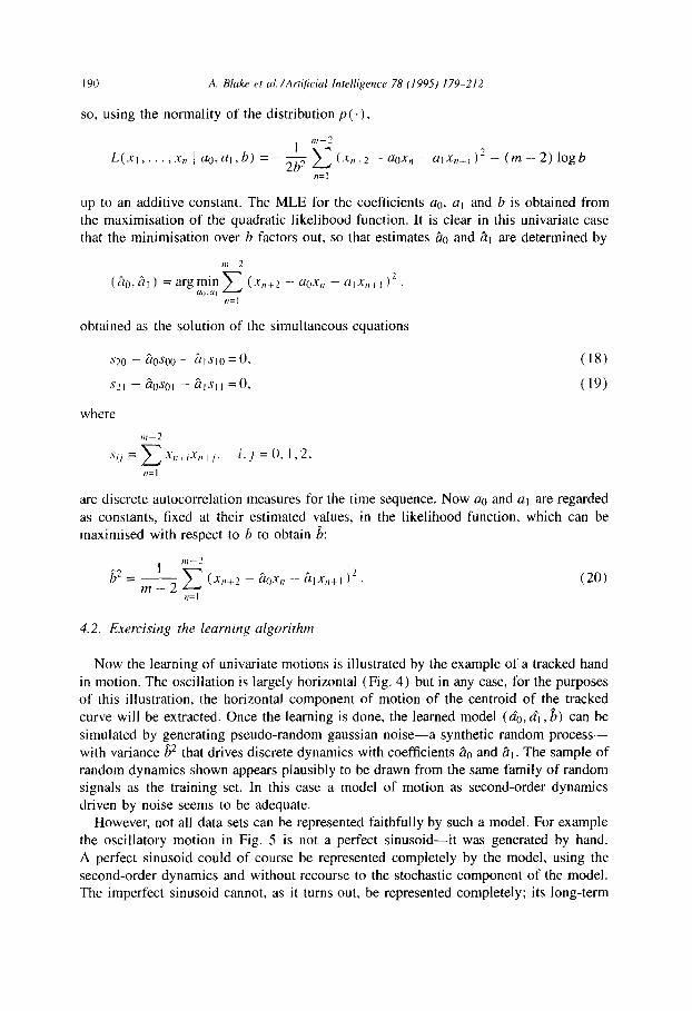
Now the learning of univariate motions is illustrated by the example of a tracked hand in motion. The oscillation is largely horizontal (Fig. 4) but in any case, for the purposes of this illustration, the horizontal component of motion of the centroid of the tracked curve will be extracted. Once the learning is done, the learned model (20, &t , &) can be
simulated by generating pseudo-random gaussian noise-a synthetic random process- with variance g2 that drives discrete dynamics with coefficients &o and 81. The sample of random dynamics shown appears plausibly to be drawn from the same family of random signals as the training set. In this case a model of motion as second-order dynamics driven by noise seems to be adequate.
However, not all data sets can be represented faithfully by such a model. For example the oscillatory motion in Fig. 5 is not a perfect sinusoid-it was generated by hand. A perfect sinusoid could of course be represented completely by the model, using the second-order dynamics and without recourse to the stochastic component of the model. The imperfect sinusoid cannot, as it turns out, be represented completely; its long-term

A. Blake et al. /Artificial Intelligence 78 (1995) 179-212 191
L b
0.1
0
0.1
radians
Fig. 4. Lmrning horizontul motion. (a) Training sequence of a tracked hand captured at 50Hz (full video field-rate) in oscillatory motion. The initial frame of the hand is shown with a subsequence of the positions of the tracked curve overlaid. The centroid’s horizontal position is displayed as a time sequence in (b). (c) Simulation of the learned system: note that the motion swept out when the learned dynamics are simulated is similar to the motion in the training set. (d) Centroid’s horizontal position for the sequence in (c). The synthesised motion appears to have reproduced a signal similar to that in the training set-observe particularly the width of the half-cycles and the amplitude of the signal,
behaviour eludes the model but its short-term behaviour, which is of particular use for prediction in trackers, is captured. The horizontal motion training set, shown as a graph in Fig. 5(b), is used in the estimation procedure of the previous section, to obtain discrete parameters a~, al and b. They can be interpreted as a damped oscillation exp -Pt exp iwt in continuous time, using Eq. (8), where p = 1.67 and w = 3.68 giving a period (27r/o) of 1.7 seconds. This is close to the apparent periodicity of the data set in which there are between 12 and 13 cycles over 20 seconds, a period of 1.54-l .67 seconds. The decay time constant of l//3 = 0.6s is not, however, apparent in the data set. It should be thought of as a coherence time constant arising because the training set does not fit our ideal model very closely: it contains the wrong kind of noise, probably closer to white noise than the integrated Brownian motion inherent in our model. Lastly, b also has a natural physical interpretation, in conjunction with the other parameters. It is the measure of the amplitude of the noise that drives the process and it can be shown that the RMS (root-mean-square) amplitude of the modelled process, in the steady

192 A. Blake et ~1. /Arti$cial Intelligence 78 (1995) 179-212
0 2 radkms
0.1 0.1
0 0
-0.1 -0.1
-0.2 V -0.2
0.2 radians
b) d)
Fig. 5. Learning horizonrul oscillufion. As for Fig. 4, but now for an oscillatory data set. (a) Training
sequence. (b) Centroid’s horizontal position. (c) and (d) As (a) and (b) but for simulation of system
learned from the training set. The synthesised motion has captured the short-term behaviour of the training set (e.g. half-cycles) but, because the motion model is limited to second-order, has not captured the phase
coherence that exists in the training set over longer time scales.
state, is a function of ae, at and b. For the model learned from this training set, the RMS amplitude is O.O6rad, which appears close to the RMS amplitude of the training set in Fig. 5.
To illustrate the learned model, we can simulate, as before. This is done with static initial conditions, not that the initial conditions have much influence beyond the first few seconds, given that the exponential-decay time constant of the system is less than one second. A sample signal, generated in this way, is shown in Figs. 5(c) and 5(d). To check for consistency, we can re-learn parameters from this synthesised signal, treating it as a training set, which gives
w. = 3.69 s-‘, p= 1.75s-‘, RMS amplitude = 0.08 rad,
which is close to the parameter set for the learned model. This indicates that the training procedure is valid, and particularly that the sequence is sufficiently long to give repeatable results.
The synthesised signal illustrates a typical sample path from our family of second- order stochastic differential equations. It is not, of course, exactly like the training

A. Blake et al./Artijicial Intelligence 78 (1995) 179-212 193
set-it is unlikely that a signal like the training set would have been produced by the simulation. However the system is the member of the family of systems that is “closest” to the training set. Broadly, the small scale properties of the training set have been captured-the period of oscillations and amplitude-but not the large-scale property of signal coherence. Clearly the model that has been learned is not a complete
one but is adequate for tracking, in which the purpose of the dynamical model is to make predictions over relatively short time scales whilst relying on data over longer
time scales. Such a model, it can be argued, is actually nzore appropriate than a more complete one which, while it may be suitable for signal recognition, would be too narrowly tuned-insufficiently general-to track a broad class of signals which is what
is required here.
4.3. Estimation of multivariate system parameters
The general multivariate estimation algorithm follows broadly the line of the univariate one, but the separability of the estimation of deterministic and stochastic parameters, whilst it still holds, is no longer so obvious. For simplicity of notation we assume that the mean a is known, and has been subtracted off:
Q-Q-e. The log-likelihood function for the multivariate normal distribution is then, up to a
constant:
Now the problem is to estimate Ao, Al and C = BBT by maximising the log-likelihood
L. Maximising first with respect to A0 and Al, it will be shown that separability holds- maxima with respect to A0 and Al turn out to be independent of the value of C. Equivalently to maximising L we minimise
L(Q,, . . . , Q, I Ao,Al,B)
= ..-i ‘E IB-’ (Q,,, - AoQ n - A,Qn+,)/’ - (m - 2) 1ogdetB. (21) n=l
m-2
f(Ao, AI) = c IB-’ (Q,,, - AoQn - 4Q,+,> I* (22) IFI
with respect to A0 and Al. Now this function can be expanded as
f(Ao,Al) =tr(ZC-I),
where
z = S22 + &&,A; + AoSooA; - &,A: - S20A; + AISloA;
-Al&2 - AoSo2 + AoSo,A:, (23)
(24)

194 A. Blake er ul./Artijicial Intelligence 78 (1995) 179-212
the second-order moment matrices for the multivariate time sequence Q,, n = I, . . . , m.
Now, completing the square in Z, with respect to both A0 and Al, we can rewrite Z as
Z(AO,AI) =Z’+Zo,
where Zc is a constant matrix, and where
Z’= (A, - &)S,,(A, -- a,)“‘+ (A0 - ~o)Soo(Ao - ao)T
+(AI ~ ii,)S,o(Ao - Ao)~ + (Ao -- ao)So,(A, - A^dT
and A0 and A^t are the solutions of the simultaneous equations
^ ^ S20 ~ AoSoo - A,Slo = 0.
1 * S,, - AoSo, - A,&, = 0.
(25)
Now a minimum of f’ exists because it is bounded below by 0. It must therefore be a positive-definite quadratic form, achieving its minimum of 0 when
A0 = Ao, A, =d,.
These conditions are independent of the value of C-the separability condition as
required. Having obtained estimators for A0 and A 1, now C can be estimated. Rewriting (21)
as
f. = -itr(ZC’) + i(m -2) IogdetC’.
fixing A0 = & and Ai = Al, and extremising with respect to C-l (using the identity d(detM)/dM = (detM)MeT) we obtain
C= -&Z(““.““.
which can be computed efficiently from (23).
(26)
4.4. Learning z,oom
As an illustration of multivariable learning, a sequence of zooming motions of a box is inferred from training data by the algorithm described above, operating over the six-dimensional planar-affine space (Fig. 6). It is instructive to examine the estimated model parameters. The zoom component of the sequence is oscillatory with a period of around 2.5 s. The modes have complex frequencies (rad/s) of
-82, -57.9, (-54.4* 1.55i), -39.8, -27.2, -9.61, -6.9,
(-4.69 -f 2.9i), (-0.54 i 2.76i)
of which the last, with the slowest decay time of around 2 seconds, has a period of 2.3 s which corresponds closely to the period of the training set, around 2.5s. The corresponding mode, expressed in the basis B, has approximately (within 5%) the form

A. Blake et al. /Artijicial Intelligence 78 (1995) 179-212 195
Fig. 6. Learning zooming morion. (a) A training sequence of 10 seconds (500 frames) duration, captured
at 50 Hz by the “default” tracker, tracks an object as it zooms inwards and outwards, spanning a family of contours as shown. This is used to estimate a system model and then to construct a tracker trained for the
zooming motion. The zoom component of the training sequence in (a) is plotted in (b) as change in scale factor versus field number (at 50 Hz). It shows a dominant period of about 2.5 seconds.
196 A. Blake et (11. /Artijicid Intelligence 78 (I 995) 179-212
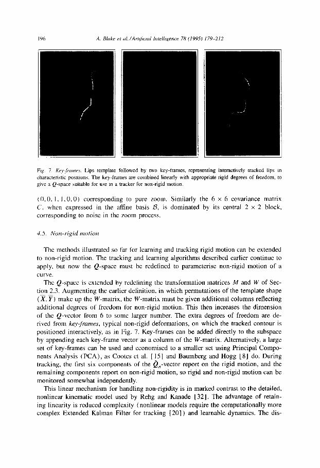
Fig. 7. Ke~Yfr~~me.~. Lips template followed by two key-frames, representing interactively tracked lips il
characteristic positions. The key-frames are combined linearly with appropriate rigid degrees of freedom, tc give a Q-space suitable for use in a tracker for non-rigid motion.
(0,O. I. I ,O,O) corresponding to pure zoom. Similarly the 6 x 6 covariance matrix C, when expressed in the affine basis 8, is dominated by its central 2 x 2 block, corresponding to noise in the zoom process.
3.5. Non-rigid motiott
The methods illustrated so far for learning and tracking rigid motion can be extended to non-rigid motion. The tracking and learning algorithms described earlier continue to apply, but now the Q-space must be redefined to parameterise non-rigid motion of a
curve. The Q-space is extended by redefining the transformation matrices M and W of Sec-
tion 2.3. Augmenting the earlier definition, in which permutations of the template shape (X, Y) make up the W-matrix, the W-matrix must be given additional columns reflecting additional degrees of freedom for non-rigid motion. This then increases the dimension of the Q-vector from 6 to some larger number. The extra degrees of freedom are de- rived from key-frames, typical non-rigid deformations, on which the tracked contour is positioned interactively, as in Fig. 7. Key-frames can be added directly to the subspace by appending each key-frame vector as a column of the W-matrix. Alternatively, a large set of key-frames can be used and economised to a smaller set using Principal Compo- nents Analysis (PCA), as Cootes et al. [ 151 and Baumberg and Hogg [ 81 do. During tracking, the first six components of the $,-vector report on the rigid motion, and the remaining components report on non-rigid motion, so rigid and non-rigid motion can be monitored somewhat independently.
This linear mechanism for handling non-rigidity is in marked contrast to the detailed, nonlinear kinematic model used by Rehg and Kanade [32]. The advantage of retain- ing linearity is reduced complexity (nonlinear models require the computationally more complex Extended Kalman Filter for tracking [ 201) and learnable dynamics. The dis-

A. Blake et al. /Artificial Intelligence 78 (1995) 179-212 197
advantage is that the linearly approximated kinematics are appropriate only for small displacements. Linear approximations are possible for larger displacements but produce underconstrained kinematic models.
5. Trained fiiters
This section investigates the effect on tracking performance of replacing default dy- namics in the predictor with specific dynamics learned from a training set. The tracking procedure for learned motions has been implemented for real-time (50 Hz) tracking on a SUN Spare-II computer with Datacell S2200 framestore, without the need for any additional hardware. It has been applied to a variety of training sequences with different objects, involving various motions, both rigid and non-rigid. Trackers have been trained for the whole affine subspace corresponding to 3D rigid motion of a hand, including translation parallel to the image plane, longitudinal motion (zoom), image plane rota- tion, and rotation about an arbitrary three-dimensional axis. They have also been trained to follow non-rigid motions both of hands and of lips.
For both rigid and non-rigid motions, tracking performance can be greatly enhanced by training. There are two contributory effects here, one static and one dynamic-one in configuration space and one in phase space. The static effect is that learning characterises
the likely configurations-both shapes and positions-of the visible contour; in the tracker this helps maintain a closer match between the tracked and the actual contour. Algorithms to learn static models have been demonstrated previously [ 15,211 but such algorithms are unable to exploit training sets that are gathered as time sequences. For static algorithms, permuting the order of elements in a training set has no effect on the
model learned. Our algorithm exploits the time sequence structure by simultaneously learning static and dynamic components of an object model. Learning is in phase space, rather than merely in configuration space. Once learned, the dynamic component of the model is used to great effect in tracking to bridge any hiatus in the measurement process, either when the target is temporarily obscured or when spatial lag is so great that the target momentarily falls outside the measurement window.
5.1. Rigid hand motion: conjiguration-space training
Three training sets are used here, each involving one component of rigid body motion, as in Fig. 8. The hand is almost planar, so the motions result in 2D affine deformations in the image plane. After training, the tracker follows motions similar to the ones in the training set, but will not follow other rigid body motions. This is illustrated in Fig. 9. Component motions of this kind can be built up individually and combined to form the predictor for a single tracker. The tracker is then tuned to follow not merely the disjunction of the component motions, but also any linear combination of them. Thus learning can be achieved in a modular fashion, and the result exhibits some degree of generalisation. How can combination of learned models be achieved? Mere concatenation of data sets for each of the individual components does not quite work because the resulting learned model would be influenced by the abrupt transitions

A. Bluke rt ~1. /Artificial Inrelli~ence 78 (I 995) 179-212
Fig. 8. Trhzing single components trf’c@k de&rmurion. (a) Hand in rest position. Training sets are shown
for: (b) zoom-hand moves towards and away from camera; (c) rotation about the line of sight; (d)
flapping-rotation about an axis parallel to the image plane.
between data sets, which are spurious. Instead, maximum likelihood estimates of system parameters are achieved by adding moments Si,; (24) from each of the data sets
s,., = c s;,;’ vi, ,j
to achieve combined moments for use in the estimation algorithm (25).
5.2. Hand tracking: phase-space training
Configuration-space training, as demonstrated above, captures only the static compo- nent of the object model. The next experiment demonstrates the power of incorporating learned dynamics into a curve tracker. This time, a training set of vertical, oscillatory, rigid motion has been generated and used to learn motion coefficients A and B, similar to the earlier example of learned horizontal motion (Section 4.2). The training set is shown in Fig. 10.
Testing of the trained tracker, incorporating the learned motion, is done against two forms of the untrained, default tracker. In both forms, translational motion is allowed

A. Blake et al./Artifcial Intelligence 78 (1995) 179-212 199
rotation data
flao data
Fig. 9. Filtering single componenfs ofa@ne deformation. The three training sets from Fig. 8 are used here to generate filters sensitive specifically to zoom, rotation and flapping. Each filter is tested on the zoom, rotation
and Rapping training sequences to illustrate the specificity of training. Accurate tracking is shown in images
along the diagonal in which each filter is run on its own training sequence. Off the diagonal, when a tuned
tracker is applied to an inappropriate test motion sequence, tracking fails.
freely. The first form is “stiff”, indicating that motion other than translation is resisted strongly-the values of p, w, p’ and W’ in ( 16) are large (/3 = 4%-l, w = 3 Is-‘, /I’ = 50~~’ and WI = 37s~’ where /3 and o govern non&fine deformations and /?’ and
w’ govern affine ones). The second form is “hard” in which those values are effectively infinite; then the shape of the estimated curve is truly rigid, having only translational degrees of freedom.
The test sequences consist of rapid, vertical, oscillatory motions of a hand. The sequences are stored on video so that fair comparisons can be made, using the standard sequences, of the performance of different trackers. Two sequences are made: one of regular oscillation against distracting background features-“clutter”, the other of oscillatory motion with gradually increasing frequency-a “chirp”. Results of the clutter

200 A. Blake et al. /Artijicial Intelligence 78 (1995) 179-212
radians
Fig. 10. Training set fiw rigid, oscillafoty, vertical motion. The centroid’s vertical position is displayed as a
time sequence, over the 25-second duration of the training sequence.
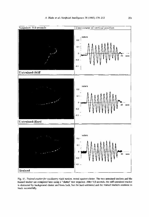
test are shown in Fig. 11. In this case the stiff-untrained tracker fails but the trained tracker succeeds. However the hard-untrained tracker also succeeds because it has a stronger shape memory than the stiff-untrained tracker. This indicates that it is the trained tracker’s learned shape, more than its learned dynamics, that enables it to track successfully in clutter. In the case of the chirp test, the results which are shown in Fig. 12 are rather different. In this test it is the rapidity of the oscillations that make tracking difficult. The trained tracker follows the motion successfully, right up to a rate of around three oscillations per second. Neither of the untrained trackers can achieve this which indicates that it is the learned dynamics of the trained tracker that enables it
to succeed here. This is confirmed by the snapshots in Fig. 12 which show that when the measurement process fails due to excessive lag in the tracker, it is the learned dynamical
model that effectively bridges the hiatus and allows lock subsequently to be recovered.
5.3. Non-rigid motion: lips
The feasibility of tracking lip movements frontally when lip highlighter is worn (Fig.
13) was demonstrated by Kass et al. [25] and our system can do this at video-rate. This paradigm can be extended by using highlighter on a number of facial features, as Terzopoulos and Waters [36] did. It is expected that this could be used with our real- time trainable tracker to build an effective front-end for actor-driven animation, without recourse to expensive virtual-reality input devices.
Tracking lips side-on, whilst arguably less informative, has the advantage of working in normal lighting condition without cosmetic aids. This could be used to turn the mouth into an additional workstation input device. Deformations of the lips for two sounds are shown in Fig. 14. Two trackers are trained individually for the sounds “Ooh” and “Pah”, and the resulting selectivity is shown in Figs. 15 and 16. It is clear from these results that the tuning effect for individual sounds is strong. Again, as in the earlier flap/zoom/rotate demonstration for rigid motion, the point is not that this particular tuning is operationally desirable, but that it demonstrates the power of the
A. Blake et al./Artificial Intelligence 78 (1995) 179-212 201
radians
Untrained-Stiff
Time-course of vertical position
radians
0.2
radians
0.2 1
Untrained-Hard
Trained
Fig. II. Trained trackerfor oscillatory rigid motion, tested against clutter. The two untrained trackers and the
trained tracker are compared here using a “clutter” test sequence. After 9.0 seconds, the stiff-untrained tracker
is distracted by background clutter and loses lock, but the hard-untrained and the trained trackers continue to track successfully.

Time-course of vertical position
Untrained-Hard I I
Fig. 12. hrnerf mrc~krr for rr,qicf t~~o~rm. rr.~/ed d/t rqd oscillations. A “chirp” test motion, consisting of
vertical oscillations of progressively increasing frequency, is tracked by each of three trackers: untrained-stiff,
untrained-hard and trained. For the untrained trackers, lock is lost after about 12 seconds and is unrecoverable
another 0.2 seconds later. The trained tracker is still tracking after 12 seconds, though it is lagging sufficiently
(more than 40 pixels, the size of the measurement window) to have lost lock. The learned model takes over
tracking temporarily. in the absence of measurements. and by 12.2 seconds lock has been recovered.
tuning process. Operationally, to render assistance to speech analysis, it is necessary to
learn the repertoire of lip motions that occurs in typical connected speech.
5.4. Cotmected speech
Now, complexity is increased by training on connected speech. Two-stage training is used. In the bootstrap stage, the default tracker follows a slow-speech training sequence which is then used, via the learning algorithm, to generate a tracker. This tracker is capable of following speech of medium speed and is used to follow a medium-speed

Fig. 13.
skin.
A. Blake et al./Artijicial Intelligence 78 (1995) 179-212 203
‘racking a frontal view of lips is possible if lip highlighter is worn, to ensure adequate contrast with
Fig. 14. Single-syllable training. Deformations of the mouth are shown corresponding to the sounds “Pah”
and “Ooh”.
training sequence, from which dynamics for a full-speed tracker are obtained. The trained tracker is then tested against the default tracker, using a test sequence entirely different from the training sequences. Two deformation components of lip motion are extracted, at 50 Hz, as “lip-reading” signals. The more significant one, in the sense that it accounts for the greater part of the lip motion, corresponds approximately to the degree to which the lips are parted. This component is plotted both for the default tracker and the partly

lntellipwe 78 (1995) 179-212
e)
b)
d)
f)
Fig. IS. Filter selecrivi~for sounds. A test sequence in which the sound “Pah” is repeated, is tracked by filters
trained on the sounds “Pah” (a) and “Ooh” (b)-the pictures show the area swept out by successive positions
of the tracked contour. Note that the “Pah” filter successfully tracks the opening/shutting deformation of the
mouth whereas only lateral translation of the head is tracked by the “Ooh” filter. The non-rigid deformation
containing the speech information is lost because a tracker trained on “Ooh” cannot accommodate deformations
associated with “Pah”. Motion signals corresponding to (a) and (b) are plotted in terms of an appropriate
scalar component of estimated motion in (c) and (d) respectively. Tracked contours approximately 4. I s after
the start of the signal are shown in (e) and (f) respectively. The signal (c) shows clear pairs of troughs
( shutting of the mouth) and peaks (opening), one pair for each “Pah”, but in (d) (tracker trained on “Ooh”)
there is minimal opening/shutting response.
and fully trained ones in Fig. 17. It is clear from the figure that the trained filter is considerably more agile. In a demonstration in which the signal is used to animate a head, the untrained filter is able to follow only very slow speech, whereas the trained filter successfully follows speech delivered at a normal speed.

A. Blake et aL/Artificial Intelligence 78 (1995) 179-212 205
b)
d)
f)
Fig. 16. Filter selecrivi@for sounds. As a companion to Fig. 15, repeated “Ooh” sounds are tracked by filters
trained on “Ooh” (a) and “Pah” (b), with corresponding motion signals in (c) and (d) and tracked contours,
approximately 5.7 s after the start of the signal, in (e) and (f) respectively. The component of motion plotted
here is different to the one in Fig. 15, now being appropriate to the “Ooh” signal. As before, the appropriately
trained filter shows a greater response. The swept motion in (b) is pure translation whereas in (a) the central
bulge in the white region indicates the deformation that accompanies the “Ooh” sound. The signal in (d) is
attenuated compared with the signal in (c) and is also noisier.
5.5. Non-rigid hand motions
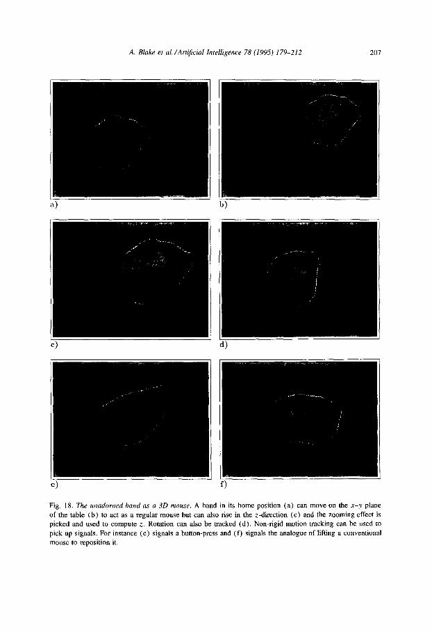
Both rigid and non-rigid motion of a hand can be used as a 3D input device. The freedom of movement of the hand is illustrated in Fig. 18, with rigid motion picked up to control 3D position and attitude, and non-rigid motion signaling button pressing and “lifting”. The tracker output-the components of 0 varying over time-have successfully been used to drive a simulated object around a 3D environment.

Un-trained lip tracker
seconds
Bootstrapped lip tracker
seconds
Fully trained lip tracker
-1~
seconds
100
Fig. 17. Ptrinetl /;/I tnrckrr. Training a tracker for side-on viewing of speaking lips greatly enhances tracking
performance. The graphs show plots from the untrained, default filter, the bootstrapped filter after one training
cycle and lastly the filter after a second training cycle. One component of deformation of the lips is shown.
corresponding to the degree to which the mouth is open-the space of deformations spanned by the first two
templates in Fig. 7. Note the considerable loss of detail in the default filter and the overshoots in both default
and bootstrapped lilters, compared with the fully trained filter. (The sentence spoken here was “In these cases
one would like to reduce the dependence of a censory information processing algorithm on these constraints
if possible.“)
5.6. F’ull K&man jilter
Finally, for the case of rigid motion of the hand, the effect of training is shown in the full Kalman filter with time-varying gains and validation gates operating on the measurement process. Allowing the validation gate to operate enhances the tracker’s
A. Blake et al. /Art$cial Intelligence 78 (1995) 179-212 207
Fig. 18. The unadorned hand as a 30 mouse. A hand in its home position (a) can move on the x-y plane
of the table (b) to act as a regular mouse but can also rise in the z-direction (c) and the zooming effect is
picked and used to compute z. Rotation can also be tracked (d). Non-rigid motion tracking can be used to
pick up signals. For instance (e) signals a button-press and (f) signals the analogue of lifting a conventional
mouse to reposition it.

20X A. Bluke ei ~11. /Art&id lntellqencr 78 (1995) 179-212
:a -
Snapshot ;tt 17.6 seconds
trained filter
Fig. 19. Trained jllll Kultrun filter. Performance in tracking of a test sequence is shown for the full
(time-varying), trained Kalman filter versus a steady-state version and an untrained version of the same
filter, Snapshots clearly show eventual failure of tracking, on a particular fixed test motion sequence, for all
except the full, trained filter-see also the next figure. (Note: validation gate is shown on either side of the
tracked curve.)

A. Blake et al./Artificial Intelligence 78 (1995) 179-212 209
Full, trained filter
Full, un-trained filter
Fig. 20. Trained fill Kalmn filter. Tracking failures for the untrained and steady-state filters, shown in the
snapshots of the previous figure, are displayed graphically here.
powers of recovery from loss of lock. Performance is reduced, not only when training is omitted (as we have already seen in numerous examples), but also when Kalman gains are fixed. This is clearly demonstrated in Figs. 19 and 20.
6. Conclusions
A new learning algorithm has been described for live tracking of moving objects from video. It supplies particular dynamics, modelled by a stochastic differential equation, to be used predictively in a contour tracker. The process is bootstrapped by a default tracker which assumes constant-velocity rigid motion driven randomly. It is crucial that
210 A. Blake et al. /Artificficlal Intelligence 78 (1995) 179-212
the constraints of rigid body motion are incorporated-represented in our algorithm by the Q-space. This is what allows stable tracking, for which the number of free parameters must be limited, to be combined with the apparently conflicting requirement that a large number of control points are needed for accurate shape representation. Rather than using
arbitrarily chosen dynamics in the tracker they are acquired by a learning algorithm that allows dynamical models to be built from examples. When such a model is incorporated into a tracker, agility and robustness to clutter are considerably increased. In the case of non-rigid motion, the learning algorithm has proved, so far, to be essential to obtaining any satisfactory tracking performance.
The advent of workstations with integral cameras and framestores (designed to fa- cilitate teleconferencing) brings an opportunity for these algorithms to be put to work. Unadorned body parts become usable input devices for graphics. This has potential applications in user-interface design, automation of animation, virtual reality, surveil- lance, the design of computer aids for the handicapped and perhaps even low-bandwidth
teleconferencing. This exploration of the learning of visual motion raises many issues. For example: how
can the acuity of the tuning of a model, or conversely its generality, be controlled? Can the learning paradigm be developed to allow model-based recognition based on visual motion, using tuned trackers as a bootstrap stage? Is it possible to learn disjunctions of motion models, either by raising the model order or by explicit model switching?
Acknowledgements
We are grateful for the use of elegant software constructed by Rupert Curwen, Nicola Ferrier, Simon Rowe, Henrik Klagges and for discussions with Mike Brady,
Roger Brockett, Yael Moses, David Mumford, Brian Ripley, Richard Szeliski, Lionel Tarassenko, Andrew Zisserman. We acknowledge the support of the AFRC (DR), the EC (MI) and the SERC ( AB) , and of the Newton Institute, Cambridge.
References
[ I 1 K.J. Astrom, fntroduction to Stochustic Control Theory (Academic Press, New York, 1970).
[ 2 1 K.J. Astrom and B. Wittenmark, Computer Controlled Systems (Addison Wesley, Reading, MA, 1984).
13) N. Ayache, I. Cohen and 1. Herlin, Medical image tracking, in: A. Blake and A. Yuille, eds., Active Vision (MIT Press, Cambridge, MA, 1992) 285-302.
141 A. Azarbayejani, T. Stamer, B. Horowitz and A. Pentland, Visually controlled graphics, IEEE Truns. &tfern Anal. Much. Intell. 15 (6) ( 1993) 602-604.
15 1 S. Bamett, Matrices: Methods and Applications (Oxford University Press, Oxford, 1990).
[ 6 1 Y. Bar-Shalom and T.E. Fortmann, Tracking and Duta Associatiun (Academic Press, New York, 1988).
[ 7 1 R.H. Bartels, J.C. Beatty and B.A. Barsky, An Introduction to Splines for Use in Computer Graphics and Geometric Modeling (Morgan Kaufmann, San Mateo, CA, 1987).
I8 1 A. Baumberg and D. Hogg, Learning flexible models from image sequences, in: J.-O. Eklundh, ed.,
Proceedings Third European Conference on Computer Vision, Stockholm, Sweden ( Springer-Verlag.
Berlin, 1994) 299-308.

A. Blake et al./Art@cial Intelligence 78 (1995) 179-212 211
191 A. Bennett and I. Craw, Finding image features for deformable templates and detailed prior statistical knowledge, in: P Mowforth, ed., Proceedings British Machine Vision Conference, Glasgow, Scotland
(Springer-Verlag, London, 1991) 233-239.
I 10 I A. Blake, J.M. Brady, R. Cipolla, Z. Xie and A. Zisserman, Visual navigation around curved obstacles. in: Proceedings IEEE International Conference on Robotics and Automation 3 ( 1991) 2490-2499.
1 111 A. Blake, R. Curwen and A. Zisserman, Affine-invariant contour tracking with automatic control 01
spatiotemporal scale, in: Proceedings Fourth International Conference on Computer Vision, Berlin
(1993) 66-75.
[ 121 A. Blake, R. Curwen and A. Zisserman, A framework for spatio-temporal control in the tracking of
visual contours, Inf. J. Comput. Vision 11 (2) (1993) 127-145.
[ 131 A. Blake and A. Yuille, eds., Active Vision (MIT Press, Cambridge, MA, 1992).
I 141 R. Cipolla and A. Blake, The dynamic analysis of apparent contours, in: Proceedings Third International Conference on Computer Vision, Osaka, Japan ( 1990) 616-625.
[ 151 T.F. Cootes, C.J. Taylor, A. Lanitis, D.H. Cooper and J. Graham, Buiding and using flexible models
incorporating grey-level information, in: Proceedings 4th International Conference on Computer Vision, Berlin ( 1993) 242-246.
[ 161 R. Curwen and A. Blake, Dynamic contours: real-time active splines, in: A. Blake and A. Yuille, eds.,
Active Vision (MIT Press, Cambridge, MA, 1992) 39-58.
1 17 1 E.D. Dickmanns and V. Graefe, Applications of dynamic monocular machine vision, Mach. Vision Appl. 1 (1988) 241-261.
[ 18 I I.D. Faux and M.J. Pratt, Computational Geometry for Design and Manufacture (Ellis-Horwood,
Chichester, England, 1979).
[ 191 M.A. Fischler and R.A. Elschlager, The representation and matching of pictorial structures, IEEE. Trans. Comput. 22 (1) (1973).
1201 A. Gelb, ed., Applied Optimal Estimation (MIT Press, Cambridge, MA, 1974).
[ 211 U. Grenander, Y. Chow and D.M. Keenan, HANDS. A Pattern Theoretical Study of Biological Shapes ( Springer-Verlag, New York, 199 1)
1221 C. Harris, Tracking with rigid models, in: A. Blake and A. Yuille, eds., Active Vision (MIT Press,
Cambridge, MA, 1992) 59-74.
1231 D. Hogg, Model-based vision: a program to see a walking person, Image Vision Comput. 1 ( 1) ( 1983)
5-20.
1241 B.K.P. Horn, Robot Vision (McGraw-Hill, New York, 1986).
[ 25 I M. Kass, A. Witkin and D. Terzopoulos, Snakes: active contour models, in: Proceedings First International Conference on Computer Vision, London (1987) 259-268.
1261 J.J. Koenderink and A.J. van Doom, Affine structure from motion, J. Optical Sot. Amer. A 8 (2) ( 1991) 337-385.
[27] D.G. Lowe, Robust model-based motion tracking through the integration of search and estimation, bit. J. Comput. Vision 8 (2) (1992) 113-122.
[ 281 S. Menet, I? Saint-Marc and G. Medioni, B-snakes: implementation and application to stereo, in:
Proceedings DARPA ( 1990) 720-726. 1291 A. Pentland and B. Horowitz, Recovery of nonrigid motion and structure, IEEE Trans. Paffern Anal.
Mach. Intell. 13 (1991) 730-742. 1301 W.H. Press, S.A. Teukolsky, W.T. Vetterling and BP. Flannery, Numerical Recipes in C (Cambridge
University Press, New York, 1988).
13 I] B.S.Y. Rao, HF. Durrant-Whyte and J.A. Sheen, A fully decentralized multi-sensor system for tracking
and surveillance, Int. J. Rob. Res. 12 (1) ( 1993) 20-44.
1321 J.M. Rehg and T. Kanade, Visual tracking of high dof articulated structures: an application to human
hand tracking, in: J.-O. Eklundh, ed., Proceedings Third European Conference on Computer Vision, Stockholm, Sweden ( Springer-Verlag. Berlin, 1994) 35-46.
I33 1 G.D. Sullivan, Visual interpretation of known objects in constrained scenes, Phil. Trans. Roy. Sot. Land.
B. 337 (1992) 109-118. [ 34 I R. Szeliski and D. Terzopoulos, Physically-based and probabilistic modeling for computer vision, in: B.C.
Vemuri, ed., Proceedings SPIE 1570, Geometric Methods in Computer Vision (Society of Photo-Optical
Instrumentation Engineers, San Diego, CA, 1991) 140-152.

212 A. Bluke et al. /Artificial Intelligence 78 (I 995) 179-212
135 1 D. Terzopoulos and D. Metaxas, Dynamic 3D models with local and global deformations: deformable
superquadrics, IEEE Trans. Pattern Anal. Mach. Intell. 13 (7) ( 1991). I36 1 D. Terzopoulos and K. Waters, Analysis of facial images using physical and anatomical models, in:
Proceedings Third International Conference on Computer Vision, Osaka, Japan (1990) 727-732.
137 1 S. Ullman and R. Basri, Recognition by linear combinations of models, IEEE Trans. Pattern Anal. Mach. Intell. 13 (10) (1991) 992-1006.
1381 A. Yuille and P Hallinan, Deformable templates, in: A. Blake and A. Yuille, eds., Active Vision (MIT
Press, Cambridge, MA, 1992) 20-38.