Learning by Similarity-weighted Imitation inWinner-takes-all Games∗

Erik Mohlin† Robert Östling‡ Joseph Tao-yi Wang§

April 6, 2018

Abstract

We study how a large population of players in the field learn to play a novelgame with a complicated and non-intuitive mixed strategy equilibrium. The gameis a winner-takes-all game with a large and ordered strategy set in which the winneris the player that chose the lowest number not chosen by anyone else. We arguethat standard models of belief-based learning and reinforcement learning are unableto explain the data, but that a simple model of similarity-based global cumulativeimitation can do so. We corroborate our findings using laboratory data from ascaled-down version of the same game, and demonstrate out-of-sample explanatorypower in three other winner-takes-all games with large and ordered strategy sets.

jel classification: C72, C73, L83.keywords: Learning; imitation; behavioral game theory; evolutionary game the-ory; stochastic approximation; replicator dynamic; similarity-based reasoning; beautycontest; lowest unique positive integer game; mixed equilibrium.

∗We are grateful for comments from Ingela Alger, Alan Beggs, Ken Binmore, Colin Camerer, Vin-cent Crawford, Ido Erev, David Gill, Yuval Heller, and Peyton Young, as well as seminar audiencesat the Universities of Edinburgh, Essex, Lund, Oxford, Warwick, and St Andrews, University CollegeLondon, the 4th World Congress of the Game Theory Society in Istanbul, the 67th European Meetingof the Econometric Society, and the 8th Nordic Conference on Behavioral and Experimental Economics.Kristaps Dzonsons (k -Consulting) and Kaidi Sun provided excellent research assistance. Erik Mohlin ac-knowledges financial support from the European Research Council (Grant no. 230251), HandelsbankensForskningsstiftelser (grant #P2016-0079:1), and the Swedish Research Council (grant #2015-01751).Robert Östling acknowledges financial support from the Jan Wallander and Tom Hedelius Foundation,and Joseph Tao-yi Wang acknowledges support from the NSC of Taiwan.†Department of Economics, Lund University. Address: Tycho Brahes väg 1, 220 07 Lund, Sweden.

E-mail: erik.mohlin@nek.lu.se.‡Institute for International Economic Studies, Stockholm University, SE—106 91 Stockholm, Sweden.

E-mail: robert.ostling@iies.su.se.§Department of Economics, National Taiwan University, 21 Hsu-Chow Road, Taipei 100, Taiwan.

E-mail: josephw@ntu.edu.tw.

1 Introduction

As pointed out already by Nash (1950), equilibria can be thought of both as the result of

deliberate optimization at the individual level, and as the end state of a process of evo-

lution or learning (the “mass-action”interpretation). There is a large literature studying

evolution and learning in games theoretically (Weibull, 1995, Hofbauer and Sigmund,

1988, Fudenberg and Levine, 1998, Sandholm, 2011), but studying mass-action learning

processes empirically in the field is challenging. The ideal test requires repeated play

of a game with well-defined rules, and the game should preferably be complicated and

dissimilar to existing games so that the game is not easily solved through individual de-

liberation or by analogical inference from experiences with similar games played in the

past. To rule out repeated-game effects, it is also desirable to study a game for which

the set of equilibrium outcomes does not expand as the game is repeated. Because these

conditions are rarely met in the field, strategic learning has rarely been studied explicitly

in the field (a recent exception is Doraszelski, Lewis and Pakes, 2018). In this paper, we

study learning using Swedish field and laboratory data from the lowest unique positive

integer (LUPI) game documented by Östling, Wang, Chou and Camerer (2011).

In the LUPI game, players simultaneously choose positive integers from 1 to K and

the winner is the player who chooses the lowest number that nobody else picked. There

are several advantages of using the field LUPI data to study strategic learning. The

game has simple and clear rules and was played for 49 consecutive days, which allows

for learning in a stable strategic environment. Repeated-game strategies are unlikely

to matter in the game because it is essentially a constant-sum game. The game has a

unique mixed strategy equilibrium which is diffi cult to compute, so it is unlikely that

players could figure it out. Moreover, the game resembles few other strategic situations

exactly, which allows us to study the behavior of truly inexperienced players who are

unlikely to be tainted by preconceived ideas formed in other similar interactions.

As shown by Östling et al. (2011), players quickly learn to play close to the equilibrum

of the LUPI game. In this paper, we use the same data, but focus on how players learn

to play equilibrium. We argue that learning in the LUPI game is best explained by a

model that assumes players imitate globally and play actions that are similar to previous

winning numbers. In contrast to most existing models that assume pair-wise imitation,

we assume each revising individual observes the payoffs of all other individuals– thereby

utilizing global information. Moreover, we assume propensities to play a particular action

are updated cumulatively, in response to how often that action, or similar actions, won

in the past. We call the resulting learning model similarity-weighted global cumulative

imitation (GCI). This simple model can explain why players so quickly come close to

equilibrium play in the LUPI game by only reacting to winning numbers.

Similarity-weighted GCI combines features from existing learning models in a novel

1

way, but the model is admittedly tailored to do the job in the LUPI game. However, we

hypothesize that the same learning model can also be used to explain learning in related

games that share some features of the LUPI game, in particular symmetric games with

large and ordered strategy sets in which at most one winning player receives a prize and

all other players earn zero. We call such games winner-takes-all games. One prominent

example belonging to this class of games is the beauty contest game (Nagel, 1995). We

also believe the model is applicable to games which award a large prize to a winner

and small non-zero payoffs to others, like the Tullock contest, all-pay auction and the

lowest unique bid auction, or other related games in which feedback is only given about

the strategy of the single player who obtains the highest payoff. In all these examples,

global imitation speeds up learning relative to simple reinforcement learning or pair-wise

imitation because in these other models only the a the winning player’s attractions are

reinforced in each round.

To test whether our learning model can explain behavior in other games than LUPI,

we test the model’s out-of-sample performance in three additional winner-takes-all games:

the second lowest unique positive integer game (SLUPI), the center-most unique positive

integer game (CUPI) and a variant of the beauty contest game (pmBC). We find that our

learning model explains behavior at least as well in SLUPI and CUPI as in the game we

designed the learning model for, LUPI. In the pmBC, convergence to equilibrum is very

rapid and our learning model only helps to explain behavior during the first few rounds

of play.

Apart from showing that the LUPI data is consistent with our proposed learning

model, we also argue that the data cannot easily be explained by existing learning models.

Reinforcement learning, i.e. learning based on reinforcement of chosen actions (e.g. Cross,

1973, Arthur, 1993, and Roth and Erev, 1995), is far too slow to be able to explain the

observed behavior in the field game. The reason is that most players never win, and hence,

their actions are never reinforced. Reinforcement learning is somewhat more successful

in the laboratory game, but as we show below, it is consistently outperformed by our own

model of learning by imitation. The leading example of belief-based learning, fictitious

play (see e.g. Fudenberg and Levine, 1998), is not applicable in the feedback environment

we study. Standard fictitious play assumes that players best respond to the average of

the past empirical distributions, but in the laboratory experiment, players only received

information about the winning number and their own payoff. In the field LUPI game

it was possible to obtain more information with some effort, but the laboratory results

suggest that this was not essential for the learning process.1 A particular variant of

fictitious play posits that players estimate their best responses by keeping track of forgone

payoffs. Again, this information is not available to our subjects, since the forgone payoff

1We nevertheless estimate a fictitious play model using the field data and find that the fit is poorerthan the imitation-based model. These results are relegated to Appendix A.

2

associated with actions below the winning number depends on the (unknown) number

of other players choosing that number. Hybrid models like EWA (Camerer and Ho,

1999, Ho, Camerer and Chong, 2007) require the same information as fictitious play and

are therefore also not applicable in this context. The myopic best response (Cournot)

dynamic suffers from similar problems.2 One may postulate players could potentially

adopt a more general form of belief-based learning with our limited feedback: players

enter the game with a prior about what strategy opponents’use, and update their beliefs

after each round in response to information about the winning number. In Appendix

A, we discuss this possibility and argue that it requires strained assumptions about the

prior distribution, as well as a high degree of forgetfulness about experiences from previous

rounds of play, in order to explain the data.

In addition to studying similarity-weighted GCI empirically, we also study the GCI

learning dynamic without similarity-weightening theoretically. Specifically, we analyze

the discrete time stochastic GCI process in LUPI and show that, asymptotically, it can

be approximated by the replicator dynamic multiplied by the expected number of players.

Using this fact, we are able to show that if the stochastic GCI process converges to a

point, then it almost surely converges to the unique symmetric Nash equilibrium of LUPI.

Moreover, we use simulations to rule other kinds of attractors, e.g. periodic orbits. The

replicator dynamic is multiplied by the expected number of players because imitation is

global. In contrast, it is well-known that reinforcement learning (and pair-wise cumulative

imitation) is approximated by the replicator dynamic without the expected number of

players as an added multiplicative factor (c.f. Börgers and Sarin, 1997, Hopkins, 2002,

and Björnerstedt and Weibull, 1996).

Our proposed learning model is most closely related to Sarin and Vahid (2004), Roth

(1995) and Roth and Erev (1995). In order to explain quick learning in weak-link games,

Sarin and Vahid (2004) add similarity-weighted learning to the reinforcement learning

model of Cross (1973), whereas Roth (1995) substitutes reinforcement learning (formally

equivalent to the model of Harley, 1981) with a model based on imitating the most

successful (highest earning) players (pp. 38—39). Similarly, Roth and Erev (1995) model

“public announcements”in proposer competition ultimatum games (“market games”) as

reinforcing the winning bid (p. 191). Relatedly, Duffy and Feltovich (1999) study whether

feedback about one other randomly chosen pair of players affects learning in ultimatum

and best-shot games. Whereas the propensity to generalize stimuli according to similarity

has been studied relatively little in strategic interactions, it is well-established in non-

strategic settings (see e.g. Shepard, 1987).

This paper is also related to unpublished work by Christensen, De Wachter and Nor-

2The myopic best response dynamic postulates that players best respond to the behavior in theprevious period. This is something that players could possibly do in the field, but still would not workin practice because the lowest unchosen number was mostly above the winning number (43 of 49 days).

3

man (2009) who study learning in LUPI laboratory experiments with rich feedback, but

they do not study imitation and find that reinforcement learning performs worse than

fictitious play. They also report field data from LUPI’s close market analogue the lowest

unique bid auction (LUBA), but their data do not allow them to study learning. The lat-

ter is also true for other papers that study LUBA, e.g. Raviv and Virag (2009), Houba,

Laan and Veldhuizen (2011), Pigolotti, Bernhardsson, Juul, Galster and Vivo (2012),

Costa-Gomes and Shimoji (2014) and Mohlin, Östling and Wang (2015).

The rest of the paper is organized as follows. Section 2 describes the equilibrium of

the games we study and the learning model. Section 3 describes and analyzes the field

and lab LUPI game. Section 4 analyzes the additional laboratory experiment that was

designed to assess the out-of-sample explanatory power of our model, and contrasts it

with reinforcement learning. Section 5 studies GCI using stochastic approximation and

discusses the related theoretical literature. Section 6 concludes the paper. A number of

appendices provide additional results as well as proofs of theoretical results.

2 Theoretical Framework

We restrict attention to winner-takes-all games in which N players simultaneously choose

integers from 1 to K. The number of players can be fixed or variable. The pure strat-

egy space is denoted S = 1, 2, ..., K and the mixed strategy space is the (K − 1)-

dimensional simplex ∆. A winner-takes-all game is defined by a mapping k∗ : SN →S ∪ ∅ that determines the winning number. All players earn zero except the player(s)choosing k∗(s). If only one player chooses k∗(s), that player earns 1, whereas one player

is randomly selected to receive 1 if more than one player choose the winning number. If

k∗(s) = ∅, all players earn zero.

2.1 Equilibrium in the LUPI Game

In the LUPI game, the lowest uniquely chosen number wins. Let U (s) denote the set of

uniquely chosen numbers under strategy profile s,

U (s) = sj ∈ s1, s2, ..., sN s.t. sj 6= sl for all sl ∈ s1, s2, ..., sN with l 6= j .

Then the winning number k∗ (s) is given by

k∗ (s) =

minsi∈U(s) si if |U (s)| 6= 0,

∅ if |U (s)| = 0.

4

Since a unique number cannot be chosen by more than one player, the payoff is

usi (s) = u (si, s−i) =

1 if si = k∗ (s) ,

0 otherwise.(1)

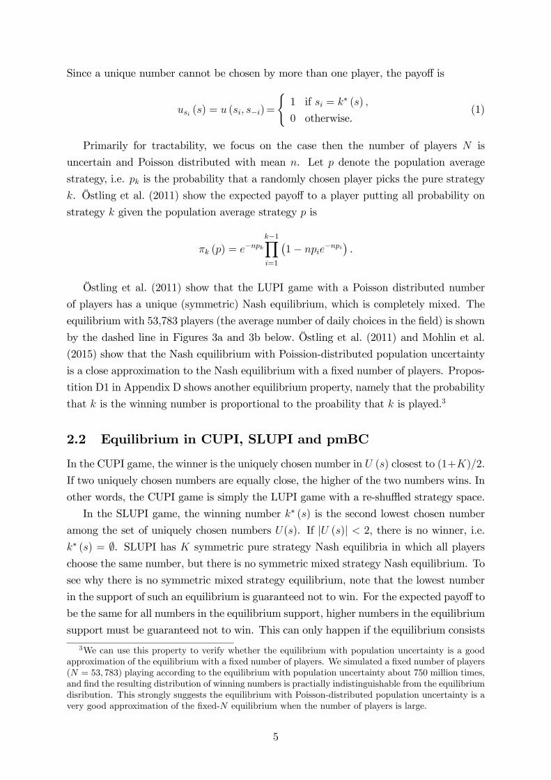
Primarily for tractability, we focus on the case then the number of players N is

uncertain and Poisson distributed with mean n. Let p denote the population average

strategy, i.e. pk is the probability that a randomly chosen player picks the pure strategy

k. Östling et al. (2011) show the expected payoff to a player putting all probability on

strategy k given the population average strategy p is

πk (p) = e−npkk−1∏i=1

(1− npie−npi

).

Östling et al. (2011) show that the LUPI game with a Poisson distributed number

of players has a unique (symmetric) Nash equilibrium, which is completely mixed. The

equilibrium with 53,783 players (the average number of daily choices in the field) is shown

by the dashed line in Figures 3a and 3b below. Östling et al. (2011) and Mohlin et al.

(2015) show that the Nash equilibrium with Poission-distributed population uncertainty

is a close approximation to the Nash equilibrium with a fixed number of players. Propos-

tition D1 in Appendix D shows another equilibrium property, namely that the probability

that k is the winning number is proportional to the proability that k is played.3

2.2 Equilibrium in CUPI, SLUPI and pmBC

In the CUPI game, the winner is the uniquely chosen number in U (s) closest to (1+K)/2.

If two uniquely chosen numbers are equally close, the higher of the two numbers wins. In

other words, the CUPI game is simply the LUPI game with a re-shuffl ed strategy space.

In the SLUPI game, the winning number k∗ (s) is the second lowest chosen number

among the set of uniquely chosen numbers U(s). If |U (s)| < 2, there is no winner, i.e.

k∗ (s) = ∅. SLUPI has K symmetric pure strategy Nash equilibria in which all players

choose the same number, but there is no symmetric mixed strategy Nash equilibrium. To

see why there is no symmetric mixed strategy equilibrium, note that the lowest number

in the support of such an equilibrium is guaranteed not to win. For the expected payoff to

be the same for all numbers in the equilibrium support, higher numbers in the equilibrium

support must be guaranteed not to win. This can only happen if the equilibrium consists

3We can use this property to verify whether the equilibrium with population uncertainty is a goodapproximation of the equilibrium with a fixed number of players. We simulated a fixed number of players(N = 53, 783) playing according to the equilibrium with population uncertainty about 750 million times,and find the resulting distribution of winning numbers is practially indistinguishable from the equilibriumdisribution. This strongly suggests the equilibrium with Poisson-distributed population uncertainty is avery good approximation of the fixed-N equilibrium when the number of players is large.

5

of two numbers, but in that case the expected payoff from playing some other number

would be positive.

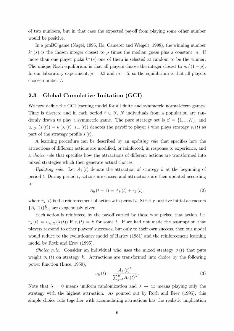
In a pmBC game (Nagel, 1995, Ho, Camerer and Weigelt, 1998), the winning number

k∗ (s) is the chosen integer closest to p times the median guess plus a constant m. If

more than one player picks k∗ (s) one of them is selected at random to be the winner.

The unique Nash equilibrium is that all players choose the integer closest to m/ (1− p).In our laboratory experiment, p = 0.3 and m = 5, so the equilibrium is that all players

choose number 7.

2.3 Global Cumulative Imitation (GCI)

We now define the GCI learning model for all finite and symmetric normal-form games.

Time is discrete and in each period t ∈ N, N individuals from a population are ran-

domly drawn to play a symmetric game. The pure strategy set is S = 1, .., K, andusi(t) (s (t)) = u (si (t) , s−i (t)) denotes the payoff to player i who plays strategy si (t) as

part of the strategy profile s (t).

A learning procedure can be described by an updating rule that specifies how the

attractions of different actions are modified, or reinforced, in response to experience, and

a choice rule that specifies how the attractions of different actions are transformed into

mixed strategies which then generate actual choices.

Updating rule. Let Ak (t) denote the attraction of strategy k at the beginning of

period t. During period t, actions are chosen and attractions are then updated according

to

Ak (t+ 1) = Ak (t) + rk (t) , (2)

where rk (t) is the reinforcement of action k in period t. Strictly positive initial attractors

Ai (1)Ki=1 are exogenously given.Each action is reinforced by the payoff earned by those who picked that action, i.e.

rk (t) = usi(t) (s (t)) if si (t) = k for some i. If we had not made the assumption that

players respond to other players’successes, but only to their own success, then our model

would reduce to the evolutionary model of Harley (1981) and the reinforcement learning

model by Roth and Erev (1995).

Choice rule. Consider an individual who uses the mixed strategy σ (t) that puts

weight σk (t) on strategy k. Attractions are transformed into choice by the following

power function (Luce, 1959),

σk (t) =Ak (t)λ∑Kj=1Aj (t)λ

. (3)

Note that λ = 0 means uniform randomization and λ → ∞ means playing only the

strategy with the highest attraction. As pointed out by Roth and Erev (1995), this

simple choice rule together with accumulating attractions has the realistic implication

6

that the learning curve flattens over time.

We also study the GCI learning dynamic using stochastic approximation, but since

these results are not directly relevant for the empirical estimation, we relegate these

results to section 5.

2.4 Similarity-weighted GCI

Throughout the paper, we restrict attention to winner-takes-all games so that at most one

action is reinforced in every period. Because only one action is reinforced every period

and we consider games with large, ordered strategy sets, reinforcing only the winning

number would result in a learning process that is slow and tightly clustered on previous

winners. Therefore, we follow Sarin and Vahid (2004) by assuming that numbers that

are similar to the winning number may also be reinforced. We use the triangular Bartlett

similarity function used by Sarin and Vahid (2004). This function implies that strategies

close to previous winners are reinforced and that the magnitude of reinforcement decreases

linearly with distance from the previous winner.

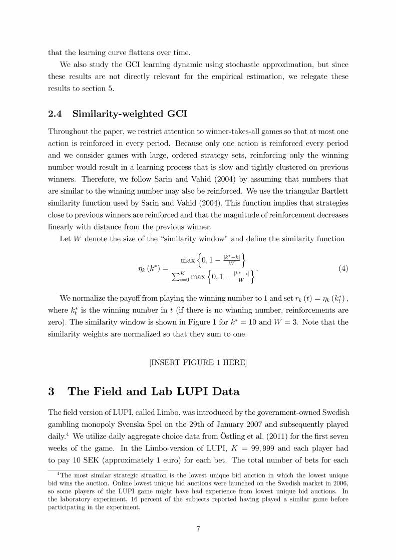
Let W denote the size of the “similarity window”and define the similarity function

ηk (k∗) =max

0, 1− |k

∗−k|W

∑K

i=0 max

0, 1− |k∗−i|W

. (4)

We normalize the payofffrom playing the winning number to 1 and set rk (t) = ηk (k∗t ) ,

where k∗t is the winning number in t (if there is no winning number, reinforcements are

zero). The similarity window is shown in Figure 1 for k∗ = 10 and W = 3. Note that the

similarity weights are normalized so that they sum to one.

[INSERT FIGURE 1 HERE]

3 The Field and Lab LUPI Data

The field version of LUPI, called Limbo, was introduced by the government-owned Swedish

gambling monopoly Svenska Spel on the 29th of January 2007 and subsequently played

daily.4 We utilize daily aggregate choice data from Östling et al. (2011) for the first seven

weeks of the game. In the Limbo-version of LUPI, K = 99, 999 and each player had

to pay 10 SEK (approximately 1 euro) for each bet. The total number of bets for each

4The most similar strategic situation is the lowest unique bid auction in which the lowest uniquebid wins the auction. Online lowest unique bid auctions were launched on the Swedish market in 2006,so some players of the LUPI game might have had experience from lowest unique bid auctions. Inthe laboratory experiment, 16 percent of the subjects reported having played a similar game beforeparticipating in the experiment.

7

player was restricted to six. The winner was guaranteed to win at least 100, 000 SEK,

but there were also smaller second and third prizes (of 1, 000 SEK and 20 SEK) for being

close to the winning number. It was possible for players to let a computer choose random

numbers for them (and cannot be disentangled from the rest). Players could access the

full distribution of previous choices through the company web site only in the form of

raw text files, so few likely looked at it. Information about winning numbers was much

more readily available on the web site and in a daily evening TV show, as well as at many

outlets of the gambling company, making it the most commonly encountered feedback.

In contrast, the laboratory LUPI data from Östling et al. (2011) follows the theory

much more closely. Their experiment consisted of 49 rounds in each session and the

prize to the winner in each round was $7. The strategy space was also scaled down

so that K = 99. The number of players in each round was drawn from a distribution

with mean 26.9.5 In the laboratory, each player was allowed to choose only one number

by themselves, there was only one prize per round, and if there was no unique number,

nobody won.6 Crucially, the only feedback that players received after each round was the

winning number. A more detailed description of the field data and laboratory experiments

can be found in Östling et al. (2011) and its Online Appendix.

3.1 Descriptive Statistics

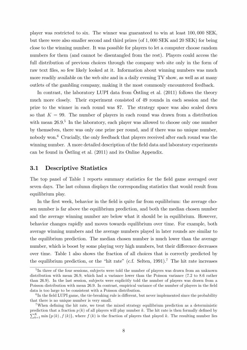
The top panel of Table 1 reports summary statistics for the field game averaged over

seven days. The last column displays the corresponding statistics that would result from

equilibrium play.

In the first week, behavior in the field is quite far from equilibrium: the average cho-

sen number is far above the equilibrium prediction, and both the median chosen number

and the average winning number are below what it should be in equilibrium. However,

behavior changes rapidly and moves towards equilibrium over time. For example, both

average winning numbers and the average numbers played in later rounds are similar to

the equilibrium prediction. The median chosen number is much lower than the average

number, which is boost by some playing very high numbers, but their difference decreases

over time. Table 1 also shows the fraction of all choices that is correctly predicted by

the equilibrium prediction, or the “hit rate”(c.f. Selten, 1991).7 The hit rate increases

5In three of the four sessions, subjects were told the number of players was drawn from an unknowndistribution with mean 26.9, which had a variance lower than the Poisson variance (7.2 to 8.6 ratherthan 26.9). In the last session, subjects were explicitly told the number of players was drawn from aPoisson distribution with mean 26.9. In contrast, empirical variance of the number of players in the fielddata is too large to be consistent with a Poisson distribution.

6In the field LUPI game, the tie-breaking rule is different, but never implemented since the probabilitythat there is no unique number is very small.

7When defining the hit rate, we treat the mixed strategy equilibrium prediction as a deterministicprediction that a fraction p (k) of all players will play number k. The hit rate is then formally defined by∑K

k=1 min p (k) , f (k), where f (k) is the fraction of players that played k. The resulting number lies

8

from about 0.45 in the first week to 0.73 in the last week. The full empirical distri-

bution, displayed in Figure 3 below, also shows clear movement towards equilibrium.

However, Östling et al. (2011) can reject the hypothesis that behavior in the last week is

in equilibrium.

Table 1. Field and lab descriptive statistics by round

All 1-7 8-14 15-21 22-28 29-35 36-42 43-49 Eq.

Field

# Bets 53783 57017 54955 52552 50471 57997 55583 47907 53783

Avg. number 2835 4512 2963 2479 2294 2396 2718 2484 2595†Median number 1675 1203 1552 1669 1604 1699 2057 1936 2542

Avg. winner 2095 1159 1906 2212 1818 2720 2867 1982 2595†Hit rate 0.64 0.45 0.59 0.65 0.65 0.68 0.73 0.73 0.87

Laboratory

Avg. number 5.96 8.56 5.24 5.45 5.57 5.45 5.59 5.84 5.22†Median number 4.65 6.14 4.00 4.57 4.14 4.29 4.43 5.00 5.00

Avg. winner 5.63 8.00 5.00 5.22 6.00 5.19 5.81 4.12 5.22†Below 20 (%) 98.02 93.94 99.10 98.45 98.60 98.85 98.79 98.42 100.00

Hit rate 0.70 0.63 0.69 0.68 0.71 0.72 0.74 0.73 0.74

†In equilibrium, the distribution of winning and chosen numbers is identical in the the LUPI game.

The bottom panel of Table 1 shows descriptive statistics for the participating subjects

in the laboratory experiment.8 As in the field, some players in the first rounds tend

to pick very high numbers (above 20) but the percentage shrinks to approximately 1

percent after the first seven rounds. Both the average and the median number chosen

corresponds closely to the equilibrium after the first seven rounds. The hit rate increases

from 0.63 during the first seven rounds to very close to the theoretical maximum in the

last 14 rounds. The overwhelming impression from the bottom panel of Table 1 is that

convergence (close) to equilibrium is very rapid despite receiving feedback only about the

winning number.9

between 0 and 1, but even if all players individually play the equilibrium mixed strategy, the empiricaldistribution will deviate from the equilibrium prediction distribution and the hit rate will be below 1.Simulations show that the expected hit rate if all players play according to the equilibrium strategy isaround 0.87 in the field and 0.74 in the lab game.

8At the beginning of each round, subjects were informed whether they were selected to activelyparticipate. Those not selected were still required to submit a number, but we focus on the choices fromincentivized subjects that were selected.

9As an additional indication of equilibrium convergence, Figure B1 in Appendix B displays the distri-bution of chosen and winning number in all sessions from period 25 and onwards. Confirming PropositionD1, the correspondence is quite close.

9

Before turning to estimation of the learning model, we analyze whether there is any

direct evidence that players imitate previous winning numbers. Figure 2 provides some

suggestive evidence that this is indeed the case in the field. Figure 2 shows how the

difference between the winning number at time t and the winning number at time t− 1

closely matches the difference between the average chosen number at time t+ 1 and the

average chosen number at time t. In other words, the average number played generally

moves in the same direction as winning numbers in the preceding periods.

[INSERT FIGURE 2 HERE]

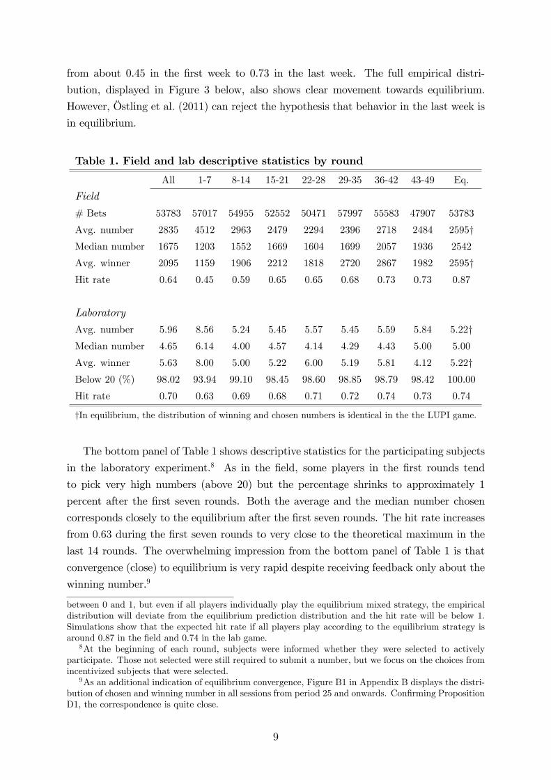
In the laboratory we test more formally whether guesses respond to previous winning

numbers. Table 2 displays the results from an OLS regression predicting changes in

average guesses with lagged differences between winning numbers. Comparing the first

14 rounds with the last 14 rounds, the estimated coeffi cients are very similar, but the

explanatory power of past winning numbers is much higher in the early rounds (R2 is

0.026 in the first 14 rounds and 0.003 in the last 14 rounds).10 Figure B2 in Appendix B

illustrates the co-movement of average guesses and previous winning numbers graphically.

Table 2. Laboratory panel data OLS regression

Dependent variable: t mean guess minus t− 1 mean guess

All periods 1—14 36—49

t− 1 winner minus t− 2 winner 0.154∗∗∗ 0.147∗∗∗ 0.172∗∗

(0.04) (0.04) (0.07)

t− 2 winner minus t− 3 winner 0.082∗ 0.089 0.169∗

(0.04) (0.05) (0.08)

t− 3 winner minus t− 4 winner 0.047 0.069 0.078

(0.03) (0.04) (0.07)

Observations 5662 1216 1710

R2 0.009 0.026 0.003

Standard errors within parentheses are clustered on individuals.

Constant included in all regressions.

3.2 Estimation Results

The similarity-weighted GCI learning model has two free parameters: the size of the

similarity window, W , and the precision of the choice function, λ. When estimating

the model, we also need to make assumptions about the choice probabilities in the first

10The reported R2 is low because the regressions are run at the level of the individual, and increasesdrastically when run at the experimental session level (0.61 for period 1—14 and 0.09 for period 36—49).

10

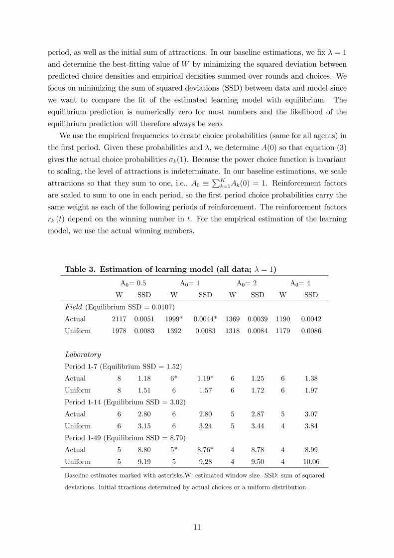
period, as well as the initial sum of attractions. In our baseline estimations, we fix λ = 1

and determine the best-fitting value of W by minimizing the squared deviation between

predicted choice densities and empirical densities summed over rounds and choices. We

focus on minimizing the sum of squared deviations (SSD) between data and model since

we want to compare the fit of the estimated learning model with equilibrium. The

equilibrium prediction is numerically zero for most numbers and the likelihood of the

equilibrium prediction will therefore always be zero.

We use the empirical frequencies to create choice probabilities (same for all agents) in

the first period. Given these probabilities and λ, we determine A(0) so that equation (3)

gives the actual choice probabilities σk(1). Because the power choice function is invariant

to scaling, the level of attractions is indeterminate. In our baseline estimations, we scale

attractions so that they sum to one, i.e., A0 ≡∑K

k=1Ak(0) = 1. Reinforcement factors

are scaled to sum to one in each period, so the first period choice probabilities carry the

same weight as each of the following periods of reinforcement. The reinforcement factors

rk (t) depend on the winning number in t. For the empirical estimation of the learning

model, we use the actual winning numbers.

Table 3. Estimation of learning model (all data; λ = 1)

A0= 0.5 A0= 1 A0= 2 A0= 4

W SSD W SSD W SSD W SSD

Field (Equilibrium SSD = 0.0107)

Actual 2117 0.0051 1999* 0.0044* 1369 0.0039 1190 0.0042

Uniform 1978 0.0083 1392 0.0083 1318 0.0084 1179 0.0086

Laboratory

Period 1-7 (Equilibrium SSD = 1.52)

Actual 8 1.18 6* 1.19* 6 1.25 6 1.38

Uniform 8 1.51 6 1.57 6 1.72 6 1.97

Period 1-14 (Equilibrium SSD = 3.02)

Actual 6 2.80 6 2.80 5 2.87 5 3.07

Uniform 6 3.15 6 3.24 5 3.44 4 3.84

Period 1-49 (Equilibrium SSD = 8.79)

Actual 5 8.80 5* 8.76* 4 8.78 4 8.99

Uniform 5 9.19 5 9.28 4 9.50 4 10.06

Baseline estimates marked with asterisks.W: estimated window size. SSD: sum of squared

deviations. Initial ttractions determined by actual choices or a uniform distribution.

11

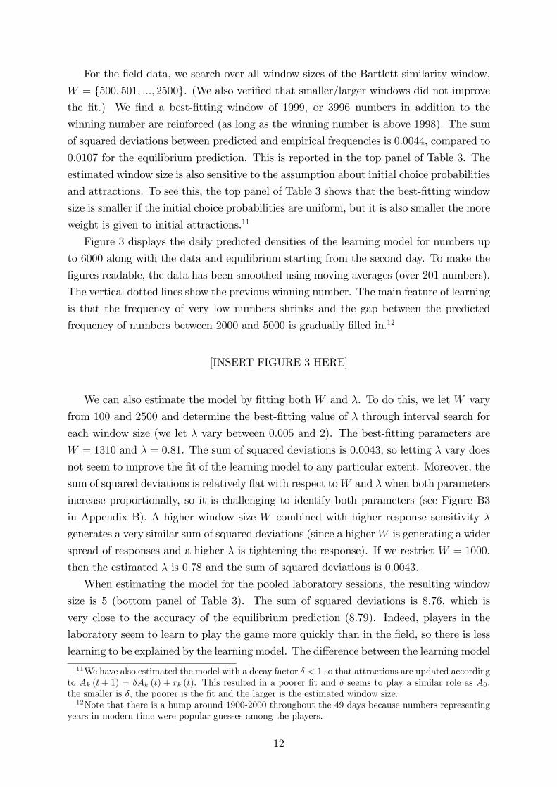
For the field data, we search over all window sizes of the Bartlett similarity window,

W = 500, 501, ..., 2500. (We also verified that smaller/larger windows did not improvethe fit.) We find a best-fitting window of 1999, or 3996 numbers in addition to the

winning number are reinforced (as long as the winning number is above 1998). The sum

of squared deviations between predicted and empirical frequencies is 0.0044, compared to

0.0107 for the equilibrium prediction. This is reported in the top panel of Table 3. The

estimated window size is also sensitive to the assumption about initial choice probabilities

and attractions. To see this, the top panel of Table 3 shows that the best-fitting window

size is smaller if the initial choice probabilities are uniform, but it is also smaller the more

weight is given to initial attractions.11

Figure 3 displays the daily predicted densities of the learning model for numbers up

to 6000 along with the data and equilibrium starting from the second day. To make the

figures readable, the data has been smoothed using moving averages (over 201 numbers).

The vertical dotted lines show the previous winning number. The main feature of learning

is that the frequency of very low numbers shrinks and the gap between the predicted

frequency of numbers between 2000 and 5000 is gradually filled in.12

[INSERT FIGURE 3 HERE]

We can also estimate the model by fitting both W and λ. To do this, we let W vary

from 100 and 2500 and determine the best-fitting value of λ through interval search for

each window size (we let λ vary between 0.005 and 2). The best-fitting parameters are

W = 1310 and λ = 0.81. The sum of squared deviations is 0.0043, so letting λ vary does

not seem to improve the fit of the learning model to any particular extent. Moreover, the

sum of squared deviations is relatively flat with respect toW and λ when both parameters

increase proportionally, so it is challenging to identify both parameters (see Figure B3

in Appendix B). A higher window size W combined with higher response sensitivity λ

generates a very similar sum of squared deviations (since a higherW is generating a wider

spread of responses and a higher λ is tightening the response). If we restrict W = 1000,

then the estimated λ is 0.78 and the sum of squared deviations is 0.0043.

When estimating the model for the pooled laboratory sessions, the resulting window

size is 5 (bottom panel of Table 3). The sum of squared deviations is 8.76, which is

very close to the accuracy of the equilibrium prediction (8.79). Indeed, players in the

laboratory seem to learn to play the game more quickly than in the field, so there is less

learning to be explained by the learning model. The difference between the learning model

11We have also estimated the model with a decay factor δ < 1 so that attractions are updated accordingto Ak (t+ 1) = δAk (t) + rk (t). This resulted in a poorer fit and δ seems to play a similar role as A0:the smaller is δ, the poorer is the fit and the larger is the estimated window size.12Note that there is a hump around 1900-2000 throughout the 49 days because numbers representing

years in modern time were popular guesses among the players.

12

and equilibrium is consequently larger in early rounds. If only the seven first rounds are

used to estimate the learning model, the best-fitting window size is 6 and the sum of

squared deviations 1.19, much smaller than the equilibrium fit of 1.52. However, since

the learning model uses actual first-period choice probabilities, this comparison is unfair.

If we instead base the initial choice probabilities of the learning model on the equilibrium

prediction, the learning model estimating using the first seven rounds improves much less

on equilibrium (1.45 vs. 1.52).

The bottom panel of Table 3 also shows the estimated window sizes for different

initial choice probabilities and weights on initial attractions. The estimated window size

is typically smaller when the initial attractions are scaled up. It is clear that our model

works best in the initial rounds of play (when most of the learning takes place). Figures

B4 to B7 in Appendix B therefore show the prediction of the learning model along with

the data and equilibrium prediction for rounds 2—6 for each session separately.

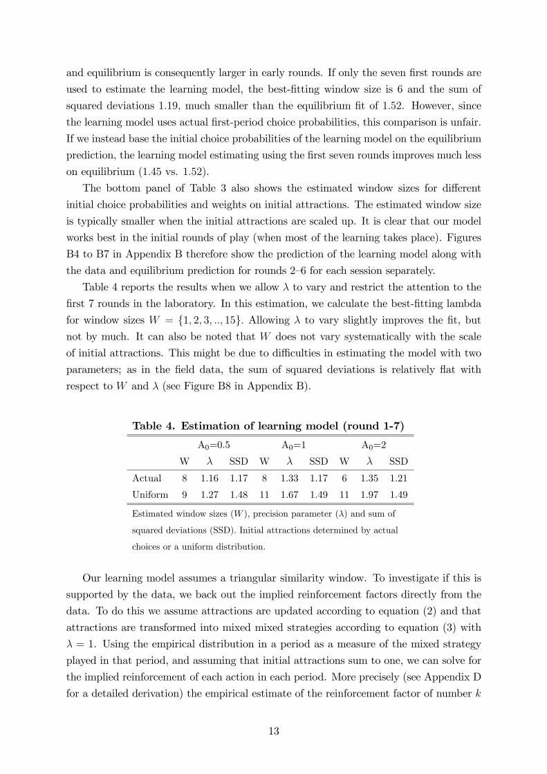
Table 4 reports the results when we allow λ to vary and restrict the attention to the

first 7 rounds in the laboratory. In this estimation, we calculate the best-fitting lambda

for window sizes W = 1, 2, 3, .., 15. Allowing λ to vary slightly improves the fit, butnot by much. It can also be noted that W does not vary systematically with the scale

of initial attractions. This might be due to diffi culties in estimating the model with two

parameters; as in the field data, the sum of squared deviations is relatively flat with

respect to W and λ (see Figure B8 in Appendix B).

Table 4. Estimation of learning model (round 1-7)

A0=0.5 A0=1 A0=2

W λ SSD W λ SSD W λ SSD

Actual 8 1.16 1.17 8 1.33 1.17 6 1.35 1.21

Uniform 9 1.27 1.48 11 1.67 1.49 11 1.97 1.49

Estimated window sizes (W ), precision parameter (λ) and sum of

squared deviations (SSD). Initial attractions determined by actual

choices or a uniform distribution.

Our learning model assumes a triangular similarity window. To investigate if this is

supported by the data, we back out the implied reinforcement factors directly from the

data. To do this we assume attractions are updated according to equation (2) and that

attractions are transformed into mixed mixed strategies according to equation (3) with

λ = 1. Using the empirical distribution in a period as a measure of the mixed strategy

played in that period, and assuming that initial attractions sum to one, we can solve for

the implied reinforcement of each action in each period. More precisely (see Appendix D

for a detailed derivation) the empirical estimate of the reinforcement factor of number k

13

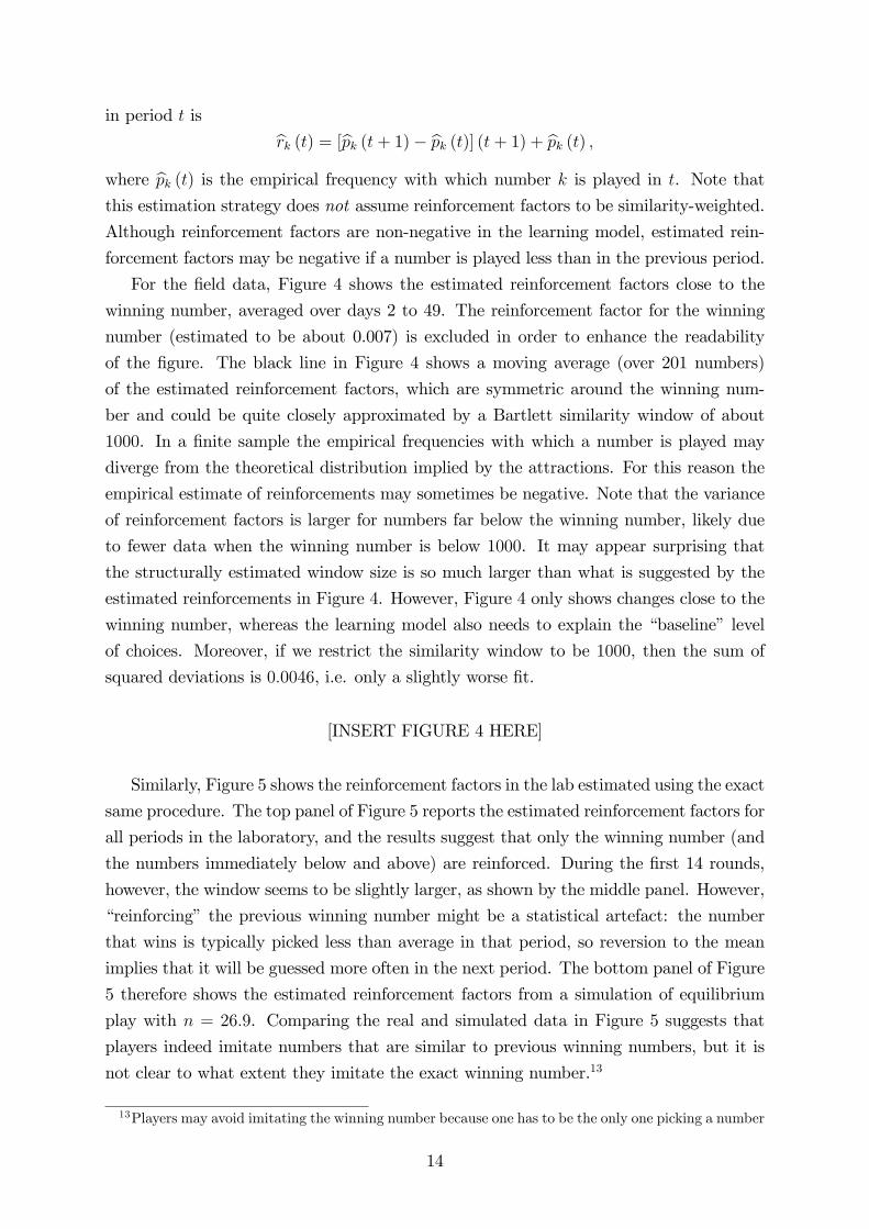
in period t is

rk (t) = [pk (t+ 1)− pk (t)] (t+ 1) + pk (t) ,

where pk (t) is the empirical frequency with which number k is played in t. Note that

this estimation strategy does not assume reinforcement factors to be similarity-weighted.

Although reinforcement factors are non-negative in the learning model, estimated rein-

forcement factors may be negative if a number is played less than in the previous period.

For the field data, Figure 4 shows the estimated reinforcement factors close to the

winning number, averaged over days 2 to 49. The reinforcement factor for the winning

number (estimated to be about 0.007) is excluded in order to enhance the readability

of the figure. The black line in Figure 4 shows a moving average (over 201 numbers)

of the estimated reinforcement factors, which are symmetric around the winning num-

ber and could be quite closely approximated by a Bartlett similarity window of about

1000. In a finite sample the empirical frequencies with which a number is played may

diverge from the theoretical distribution implied by the attractions. For this reason the

empirical estimate of reinforcements may sometimes be negative. Note that the variance

of reinforcement factors is larger for numbers far below the winning number, likely due

to fewer data when the winning number is below 1000. It may appear surprising that

the structurally estimated window size is so much larger than what is suggested by the

estimated reinforcements in Figure 4. However, Figure 4 only shows changes close to the

winning number, whereas the learning model also needs to explain the “baseline” level

of choices. Moreover, if we restrict the similarity window to be 1000, then the sum of

squared deviations is 0.0046, i.e. only a slightly worse fit.

[INSERT FIGURE 4 HERE]

Similarly, Figure 5 shows the reinforcement factors in the lab estimated using the exact

same procedure. The top panel of Figure 5 reports the estimated reinforcement factors for

all periods in the laboratory, and the results suggest that only the winning number (and

the numbers immediately below and above) are reinforced. During the first 14 rounds,

however, the window seems to be slightly larger, as shown by the middle panel. However,

“reinforcing” the previous winning number might be a statistical artefact: the number

that wins is typically picked less than average in that period, so reversion to the mean

implies that it will be guessed more often in the next period. The bottom panel of Figure

5 therefore shows the estimated reinforcement factors from a simulation of equilibrium

play with n = 26.9. Comparing the real and simulated data in Figure 5 suggests that

players indeed imitate numbers that are similar to previous winning numbers, but it is

not clear to what extent they imitate the exact winning number.13

13Players may avoid imitating the winning number because one has to be the only one picking a number

14

[INSERT FIGURE 5 HERE]

4 Out-of-sample Explanatory Power

Similarity-weighted GCI seems to be able to capture how players in both the field and

the laboratory learn to play the LUPI game. However, the learning model was developed

after observing Östling et al’s (2011) LUPI data, which raises worries that the model is

only suited to explain learning in this particular game. Therefore, we conducted new

experiments with SLUPI, CUPI and pmBC. We selected games with large, ordered strat-

egy sets so that similarity-weighted learning makes sense. We also choose games with

relatively complex rules so that it would not be transparent to calculate best responses.

We made no changes to the similarity-weighted GCI model after observing the results

from these games.

4.1 Experimental Design

Experiments were run at the Taiwan Social Sciences Experimental Laboratory (TASSEL),

National Taiwan University in Taipei, Taiwan, during June 23-27, 2014. We conducted

three sessions with 29 or 31 players in each session. In each session, all subjects actively

participated in 20 rounds of each of the three games described above. The order of the

games varied across sessions: CUPI-pmBC-SLUPI in the first session (June 23), pmBC-

CUPI-SLUPI in the second (June 25) and SLUPI-pmBC-CUPI in the third session (June

27). The prize to the winner in each round was NT$200 (approximately US$7 at the

time of the experiment). Each subject was informed, immediately after each round,

what the winning number was (in case there was a winning number), whether they had

won in that particular round, and their payoff so far during the experiment. There

were no practice rounds. All sessions lasted for less than 125 minutes, and the subjects

received a show-up fee of NT$100 (approximately US$3.5) in addition to earnings from the

experiment (which averaged NT$380.22, ranging from NT$0 to NT$1200). Experimental

instructions translated from Chinese are available in Appendix C. The experiments were

conducted using the experimental software zTree 3.4.2 (Fischbacher, 2007) and subjects

were recruited using the TASSEL website.

4.2 Descriptive Statistics

Figure 6 shows how subjects played in the first and last five rounds in the three different

games. The black lines show the mixed equilibrium of the CUPI game (with 30 players).

to win. Estimating a learning model where players do not imitate winning numbers, but only numbersclose to it yields slightly worse fit.

15

Since there is no obvious theoretical benchmark for the SLUPI game, we instead simulate

20 rounds of the similarity-weighted GCI 100,000 times and show the average prediction

for the last round. In this simulation, we set λ = 1 and use the best-fitting window

size for the first 20 rounds of the LUPI laboratory experiment (W = 5). The initial

attractions were uniform.

[INSERT FIGURE 6 HERE]

It is clear from Figure 6 that players learn to play close to the theoretical benchmark

in all three games. The learning pattern is particularly striking in the pmBC game: in

the first period, 9% play the equilibrium strategy, which increases to 62% in round 5 and

95% in round 10. In the CUPI game, subjects primarily learn not to play 50 so much —

in the first round 26 percent of all subjects play 50 —and there are fewer guesses far from

50. In the SLUPI game, it is less clear how behavior changes over time, but it is clear

that there are fewer very high choices in the later periods.

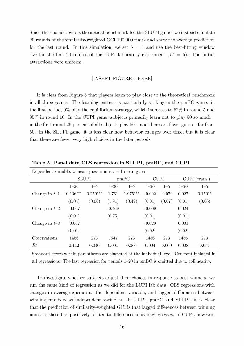
Table 5. Panel data OLS regression in SLUPI, pmBC, and CUPI

Dependent variable: t mean guess minus t− 1 mean guess

SLUPI pmBC CUPI CUPI (trans.)

1—20 1—5 1—20 1—5 1—20 1—5 1—20 1—5

Change in t—1 0.136∗∗∗ 0.259∗∗∗ 1.761 1.975∗∗∗ -0.022 -0.079 0.027 0.150∗∗

(0.04) (0.06) (1.91) (0.49) (0.01) (0.07) (0.01) (0.06)

Change in t—2 -0.007 -0.469 -0.009 0.024

(0.01) (0.75) (0.01) (0.01)

Change in t—3 -0.007 - -0.020 0.031

(0.01) - (0.02) (0.02)

Observations 1456 273 1547 273 1456 273 1456 273

R2 0.112 0.040 0.001 0.066 0.004 0.009 0.008 0.051

Standard errors within parentheses are clustered at the individual level. Constant included in

all regressions. The last regression for periods 1—20 in pmBC is omitted due to collinearity.

To investigate whether subjects adjust their choices in response to past winners, we

run the same kind of regression as we did for the LUPI lab data: OLS regressions with

changes in average guesses as the dependent variable, and lagged differences between

winning numbers as independent variables. In LUPI, pmBC and SLUPI, it is clear

that the prediction of similarity-weighted GCI is that lagged differences between winning

numbers should be positively related to differences in average guesses. In CUPI, however,

16

it is possible that players instead imitate numbers that are similar in terms of distance

to the center rather than similar in terms of actual numbers. Therefore, we also report

the results after transforming the strategy space. In this transformation, we re-order the

strategy space by distance to the center so that 50 is mapped to 1, 51 to 2, 49 to 3, 52

to 4 and so on. The reason we use this asymmetric transformation rather than simply

using the distance to 50 is that our tie-breaking rule is slighly asymmetric; if two numbers

are uniquely chosen then the higher number wins. The regression results are reported in

Table 5.

In SLUPI and pmBC, it is clear that guesses move in the same direction as the

winning number in the previous round during the first five rounds. After the initial five

rounds, this tendency is less clear, especially in the pmBC game where players learn

to play equilibrium very quickly. In the CUPI, subjects seem to imitate based on the

transformed strategy set rather than actual numbers. In the remainder, we therefore

report CUPI results with the transformed strategy space. Again, the tendency to imitate

is strongest during the first five rounds. It is primarily during these first periods that

we should expect our model to predict well, because learning slows down after the initial

periods. The effect of winning numbers on chosen numbers in pmBC, CUPI and SLUPI

is illustrated in Figure B9 in Appendix B.

We also estimate the reinforcement factors following the same procedure as in LUPI.

The result when all periods are included is shown in Figure 7. Since there is most clear

evidence of imitation in early rounds, Figure B10 in Appendix B reports the corresponding

estimation when restricting the attention to periods 1-5 only. Figure 7 indicates that there

is a triangular singularity window in both SLUPI and CUPI. As Figure B10 reveals,

however, this is less clear in early rounds —players seem to avoid imitating the exact

winning number from the previous round. In pmBC, players are predominantly playing

the previous winning number which is due to the fact that most players always play

equilibrium after the fifth round. When restricting the attention to the first five periods,

estimated reinforcement has a triangular shape, although it is clear that players primarily

imitate the winning number and numbers below the winning number.

[INSERT FIGURE 7 HERE]

4.3 Estimation Results

The results in the previous section suggest that the similarity-weighted GCI model might

be able to explain the learning pattern observed in the data. To verify this, we set λ = 1

and fixed the window size atW = 5, which was the best-fitting window size for the first 20

periods in the laboratory LUPI game. As in our baseline estimation for the LUPI game,

17

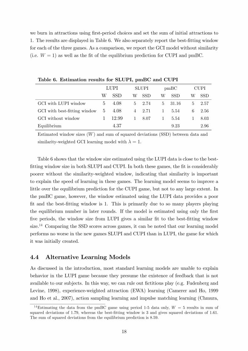
we burn in attractions using first-period choices and set the sum of initial attractions to

1. The results are displayed in Table 6. We also separately report the best-fitting window

for each of the three games. As a comparison, we report the GCI model without similarity

(i.e. W = 1) as well as the fit of the equilibrium prediction for CUPI and pmBC.

Table 6. Estimation results for SLUPI, pmBC and CUPI

LUPI SLUPI pmBC CUPI

W SSD W SSD W SSD W SSD

GCI with LUPI window 5 4.08 5 2.74 5 31.16 5 2.57

GCI with best-fitting window 5 4.08 4 2.71 1 5.54 6 2.56

GCI without window 1 12.99 1 8.07 1 5.54 1 8.03

Equilibrium 4.37 9.23 2.96

Estimated window sizes (W ) and sum of squared deviations (SSD) between data and

similarity-weighted GCI learning model with λ = 1.

Table 6 shows that the window size estimated using the LUPI data is close to the best-

fitting window size in both SLUPI and CUPI. In both these games, the fit is considerably

poorer without the similarity-weighted window, indicating that similarity is important

to explain the speed of learning in these games. The learning model seems to improve a

little over the equilibrium prediction for the CUPI game, but not to any large extent. In

the pmBC game, however, the window estimated using the LUPI data provides a poor

fit and the best-fitting window is 1. This is primarily due to so many players playing

the equilibrium number in later rounds. If the model is estimated using only the first

five periods, the window size from LUPI gives a similar fit to the best-fitting window

size.14 Comparing the SSD scores across games, it can be noted that our learning model

performs no worse in the new games SLUPI and CUPI than in LUPI, the game for which

it was initially created.

4.4 Alternative Learning Models

As discussed in the introduction, most standard learning models are unable to explain

behavior in the LUPI game because they presume the existence of feedback that is not

available to our subjects. In this way, we can rule out fictitious play (e.g. Fudenberg and

Levine, 1998), experience-weighted attraction (EWA) learning (Camerer and Ho, 1999

and Ho et al., 2007), action sampling learning and impulse matching learning (Chmura,

14Estimating the data from the pmBC game using period 1-5 data only, W = 5 results in sum ofsquared deviations of 1.79, whereas the best-fitting window is 3 and gives squared deviations of 1.61.The sum of squared deviations from the equilibrium prediction is 8.59.

18

Goerg and Selten, 2012), and myopic best response (Cournot) dynamic. These observa-

tions also apply to SLUPI and CUPI, whereas there are several possible learning models

that can explain learning in the pmBC. In Appendix A, we demonstrate that more gen-

eral forms of Bayesian learning are also unable to explain observed behavior in LUPI,

unless very specific assumptions are made, and we also estimate a fictitious play model

using the field data.

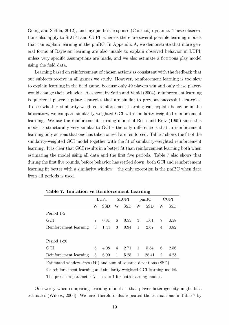
Learning based on reinforcement of chosen actions is consistent with the feedback that

our subjects receive in all games we study. However, reinforcement learning is too slow

to explain learning in the field game, because only 49 players win and only these players

would change their behavior. As shown by Sarin and Vahid (2004), reinforcement learning

is quicker if players update strategies that are similar to previous successful strategies.

To see whether similarity-weighted reinforcement learning can explain behavior in the

laboratory, we compare similarity-weighted GCI with similarity-weighted reinforcement

learning. We use the reinforcement learning model of Roth and Erev (1995) since this

model is structurally very similar to GCI —the only difference is that in reinforcement

learning only actions that one has taken oneself are reinforced. Table 7 shows the fit of the

similarity-weighted GCI model together with the fit of similarity-weighted reinforcement

learning. It is clear that GCI results in a better fit than reinforcement learning both when

estimating the model using all data and the first five periods. Table 7 also shows that

during the first five rounds, before behavior has settled down, both GCI and reinforcement

learning fit better with a similarity window —the only exception is the pmBC when data

from all periods is used.

Table 7. Imitation vs Reinforcement Learning

LUPI SLUPI pmBC CUPI

W SSD W SSD W SSD W SSD

Period 1-5

GCI 7 0.81 6 0.55 3 1.61 7 0.58

Reinforcement learning 3 1.44 3 0.94 1 2.67 4 0.82

Period 1-20

GCI 5 4.08 4 2.71 1 5.54 6 2.56

Reinforcement learning 3 6.90 1 5.25 1 28.41 2 4.23

Estimated window sizes (W ) and sum of squared deviations (SSD)

for reinforcement learning and similarity-weighted GCI learning model.

The precision parameter λ is set to 1 for both learning models.

One worry when comparing learning models is that player heterogeneity might bias

estimates (Wilcox, 2006). We have therefore also repeated the estimations in Table 7 by

19

fitting individual-specific similarity windows. In this estimation, we estimate the best-

fitting window size Wi separately for each subject i by minimizing the sum of squared

deviations between the learning model’s prediction and the subject’s choices. The average

estimated window sizes are similar to those reported in Table 7, and GCI always has a

better fit than reinforcement learning.

5 Stochastic Approximation of GCI

Our empirical results suggest imitation learning converges to equilibrium in the LUPI

game (as well as in the three games used for out-of-sample testing). In this section,

we study the GCI learning theoretically to investigate whether movement towards equi-

librium is merely a coincidence in our data, or whether it is an inherent property of

the learning dynamic, focusing on LUPI. We derive analytical results for GCI with-

out similarity-weighted imitation, and under the assumption that λ = 1. We discuss

similarity-weighed GCI separately in section 5.4.

5.1 GCI in Winner-takes-all Games

The updating and choice rules described in section 2.3 together define a stochastic process

on the set of mixed strategies (i.e. the probability simplex). Since new reinforcements

are added to old attractions, the relative importance of new reinforcements will decrease

over time. This means that the stochastic process moves with smaller and smaller steps.

Under certain conditions, the stochastic process will eventually behave approximately

like a deterministic process. By finding an expression for this deterministic process, and

studying its convergence properties, we are able to infer convergence properties of the

original stochastic process.

Recall that p denotes the population average strategy. To simplify the exposition we

assume that all individuals have the same initial attractions, so that all individuals play

the same strategy, i.e. we assume

pk (t) =Ak (t)λ∑Kj=1Aj (t)λ

.

As we demonstrate in Appendix D, this assumption can be relaxed, to allow individual i

to follow strategy σi and letting p be the average strategy in the population. The reason

why this can be done is that all players asymptotically play according to the same strategy

because all individuals reinforce the same strategy in all periods and initial attractions

are therefore washed out asymptotically.

In order to apply the relevant stochastic approximation techniques, we need rein-

forcements to be strictly positive. We do this by adding a constant c > 0, so that all

20

subjective utilities are strictly positive (c.f. Gale, Binmore and Samuelson, 1995). We

define reinforcements as follows

rk (t) =

usi(t) (s (t)) + c if si (t) = k for some i,

c otherwise.(5)

The addition of the constant c can be viewed as a way to represent noise in the perception

of payoffs. The constant c must be strictly positive for the stochastic approximation

argument to go through, but can be made arbitrarily small (see Appendix D, remark

D1).15

The stochastic process moves in discrete time. In order to be able to compare it with

a deterministic process that moves in continuous time, we consider the interpolation of

the stochastic process. The following proposition ties together the interpolated process

with a deterministic process.16

Proposition 1 Consider the class of winner-takes-all games with a Poisson distributednumber of players. Define the continuous time interpolated stochastic GCI process p :

R+ → ∆ by

p (t+ s) = p (t) + sp (t+ 1)− p (t)

1/ (t+ 1),

for all n ∈ N and 0 ≤ s ≤ 1/ (t+ 1). With probability 1, every ω-limit set of p is a

compact invariant set A ⊂ ∆ that admits no proper attractor, under the flow Φ induced

by the following continuous time deterministic GCI dynamic

pk = npk

(πk (p)−

K∑j=1

pjπj (p)

)+ c (1−Kpk) . (6)

15An alternative to adding positive constants to reinforcements is to add the same constant to allpayoffs, resulting in a game that is strategically equivalent to the original game (but where all payoffsare strictly positive) and then define reinforcements without addition of the constant. This works in thecase of reinforcement learning, see e.g. Hopkins and Posch (2005). However, this strategy does not workin the case of GCI since players are unable to distinguish those actions which were chosen by others butlost, from those actions that were not chosen by anyone. As a consequence we need to study a perturbedreplicator dynamic below.16We borrow the following notation and definitions from Benaïm (1999). Consider a metric space

(X, d) (in our case it is the simplex ∆ and Euclidean distance) and a semi-flow Φ : R+×X → X inducedby a vector field F on X. A point x ∈ X is a rest point (an equilibrium in Benaïm’s terminology) ifΦt (x) = x for all t. A point x∗ ∈ X is an ω-limit point of x if x∗ = limtk→∞ Φtk (x) for some sequencetk → ∞. Intuitively, an ω-limit point of x is a point to which the semi-flow Φt (x) always returns. Theω-limit set of x, denoted ω (x), is the set of ω-limit points of x. The definition of an ω-limit can beextended to a discrete time system. A set A ⊆ X is invariant if Φt (A) = A for all t ∈ R. A subsetA ⊆ X is an attractor for Φ if (i) A is non-empty, compact and invariant, and (ii) A has a neighborhoodU ⊆ X such that limt→∞ d (Φt, A) → 0 uniformly in x ∈ U (the distance between Φt and the closestpoint in A). An attractor A is a proper attractor if it contains no proper subset that is an attractor.The study of this kind of stochastic processes was initiated by Robbins and Monro (1951). The

ODE method originates with Ljung (1977). For a book-length treatment of the theory of stochasticapproximation, see Benveniste, Priouret and Métivier (1990).

21

Equation (6) is the replicator dynamic (Taylor and Jonker, 1978) multiplied by n plus

a noise term due to the addition of the constant c to all reinforcements. The replicator

dynamic is arguably the most well studied deterministic dynamic within evolutionary

game theory (Weibull, 1995). Börgers and Sarin (1997) and Hopkins (2002) use sto-

chastic approximation to derive the replicator dynamic, without the multiple n, from

reinforcement learning with decreasing step-size. Björnerstedt and Weibull (1996) (see

also Weibull, 1995, Section 4.4) derive the replicator dynamic (without the multiple n)

from learning by pairwise imitation in the large population limit learning. Similarly, we

can define pair-wise (cumulative) imitation, and obtain the replicator dynamic (without

the multiple n) in the limit as step-size decreases.17 Thus we have found that global im-

itation leads to a faster learning process, and hence potentially faster convergence, than

either reinforcement learning or pairwise cumulative imitation.

Remark 1 Proposition 1 concerns games with a Poisson-distributed number of players.If the number of players is fixed and equal to N , then we will still obtain the same

expression for the continuous time deterministic GCI dynamic (with N in place of n)

in the limit as c→ 0. This follows from propositions E1 and E2 in Appendix E.

5.2 GCI in LUPI

The unique symmetric Nash equilibrium of the LUPI game is the unique interior rest

point of the unperturbed replicator dynamic,

pk = npk

(πk (p)−

K∑j=1

pjπj (p)

). (7)

Our next result, Proposition 2, establishes that (part 1) for small enough noise levels the

perturbed replicator dynamic (6) has a unique interior rest point. Thus, (part 2) if the

GCI-process converges to an interior point, then it converges to the unique interior rest

point of the perturbed replicator dynamic. In addition to the unique interior rest point,

the unperturbed replicator dynamic (7) has rest points on the boundary of the simplex.

However, it can be shown that (part 2) the stochastic GCI process almost surely does

not converge to the boundary. These results hold for the CUPI game as well since it’s

strategy space is merely a permutation of the strategy space of the LUPI game.

17We can define pair-wise (cumulative) imitation for a setting with decreasing step-size as follows. Asbefore we assume that strictly positive initial attractors Ai (1)Ki=1 are exogenously given, let attractionsbe updated according to (2), and let the choice rule be (3). We define reinforcement factors in a differentway than before. In every period each agent draws one other player as role model and reinforces theaction taken by that role model with the payoff earned by the role model. For the same reasons as beforewe add a constant c to all payoffs. Since the probability of that an action k wins is independent of thetotal number of players that are realised in a given period, the expected reinforcement is 1nE [rk (t) |Ft] =pk (t)πk (p (t)) + c

n . Plugging this into equation (D3) in Appendix D gives us the replicator dynamic(without a multiple n) plus a noise term.

22

Proposition 2 There is some c such that if c < c then the following holds.

1. The perturbed replicator dynamic (6) has a unique interior rest point pc∗.

2. If the stochastic GCI process converges to an interior point, then it converges to the

unique interior rest point pc∗ of the perturbed replicator dynamic.

3. The stochastic GCI process almost surely does not converges to a point on the bound-

ary, i.e. for all k, Pr (limt→∞ pk (t) = 0) = 0.

Thus, we know that if the stochastic GCI process converges to a point, then it must

converge to the unique interior rest point of the perturbed replicator dynamic (6), which

as c→ 0, moves arbitrarily close to the Nash equilibrium of LUPI. Our empirical results

suggests that learning converges to a point in the simplex. Proposition 2 then implies

that if subjects learn by GCI, we should see convergence to the equilibrium (or a c-

perturbed version thereof), which is consistent with what the data indicate (especially in

the laboratory).

The results in Proposition 2 do not preclude the theoretical possibility that the sto-

chastic GCI-process could converge to something else than a point, e.g. a periodic orbit.

In order to check whether this possibility can be ignored, we simulated the learning

process. We used the lab parameters K = 99 and n = 26.9, and randomly drew 100

different initial conditions. For each initial condition, we ran the process for 10 million

rounds. The simulated distribution is virtually indistinguishable from the equilibrium

distribution except for the numbers 11-14, where some minor deviations occur. This is

illustrated in Figure F1 in Appendix F. It strongly indicates global convergence of the

stochastic GCI process in LUPI.

In Appendix F, we also study the local stability properties of the unique interior

rest point by combining analytical and numerical methods. Analytically, we establish

that local stability under the perturbed dynamic is guaranteed if all the eigenvalues of a

particular matrix are negative. Furthermore, if this holds then the equilibrium p∗ is an

evolutionarily stable strategy. Due to the nonlinearity of payoffs we are only able to check

the eigenvalues with the help of numerical methods, and even for a computer this is only

possible to do for the parameter values from the laboratory version of LUPI; not for the

parameter values in the field. For the laboratory parameter values we do indeed find that

all eigenvalues are negative. This implies that, p∗ is an evolutionarily stable strategy, and

with positive probability the stochastic GCI-process converges to the unique interior rest

point of the perturbed replicator dynamic, at least for the parameters of the laboratory

LUPI game.

23

5.3 GCI for General Games

In LUPI, as well as the other winner-takes-all games we study, there is no difference

between imitating only the highest earners, and imitating everyone in proportion to their

earnings. This is due to the fact that in every round, at most one person earns more

than zero. For the same reasons, there is also no difference between imitation which is

solely based on payoffs, and imitation which is sensitive both to payoffs and to how often

actions are played.

To extend the application of the GCI model beyond winner-takes-all games, we need

to calculate expected reinforcement more generally. This requires us to make two distinc-

tions. First, imitation may or may not be responsive to the number of people who play dif-

ferent strategies, so we distinguish frequency-dependent (FD) and frequency-independent

(FI) versions of GCI. For simplicity, we assume a multiplicative interaction between pay-

offs and frequencies, i.e. reinforcement in the frequency-dependent model depends on

the total payoff of all players that picked an action. Second, imitation may be exclu-

sively focused on emulating the winning action, i.e. the action that obtained the highest

payoff, or be responsive to payoff-differences in a proportional way, so we differentiate

between winner—takes-all imitation (W) and payoff-proportional imitation (P). In total,

we propose the following four members of the GCI family: PFI, PFD,WFD, andWFI.18

In Appendix E, we discuss these different versions of GCI in greater detail. In partic-

ular, we show that in winner-takes-all games, they all coincide if the number of players

is Poisson distributed. Furthermore, we show that, in general, it is only the payoff-

proportional and frequency-dependent version (PFD) of GCI that induces the replicator

dynamic multiplied by the expected number of players as its associated continuous time

dynamic. PFD can be used in information environments where there is population-wide

information available about both payoffs and frequencies of different actions. In such

settings it generates more rapid learning than either pairwise imitation or reinforcement

learning, as described above.

5.4 Similarity-weighted GCI

In Appendix E we show that similarity-weighted GCI in LUPI does not result in the

replicator dynamic (Proposition E3) and that the Nash equilibrium is not a rest point.

We therefore instead simulate the similarity-weighted GCI process to examine whether

it converges, and how the limit point differs from the Nash equilibrium. We use the

laboratory parameters, K = 99 and n = 26.9, and randomly draw 100 different initial

conditions. For each initial condition and windows sizes W = 3 and W = 6, we simulate

18The information environment is likely to affect which learning heuristic will be used. For example,sometimes information is rich enough to make it possible to infer how common different behaviors are(e.g. how many firms that entered a particular industry), whereas such inference is not possible at othertimes (e.g. it is often diffi cult to know how many firms that use a particular business practice).

24

the learning model for 100, 000 rounds. Figure E1 shows the resulting distribution of end

states averaged over the 100 initial conditions. The process does seem to converge, but

as expected it does not converge to the Nash equilibrium. For the smaller window size,

W = 3, the end state is very close to equilibrium, whereas it is a bit further away from

equilibrium for the larger window size W = 6, although the shape of the distribution

is quite similar. Recall that the best-fitting window size was W = 5 in our estimations

above. Thus at least for the lab parameters, adding similarity weights does not seem to

affect the qualitative insigts gained from the model without similarity window.

In Appendix E we also generalize the similarity-weighted GCI model beyond LUPI.

We show that if reinforcements are payoff-proportional and frequency-dependent, then

the similarity-weighted GCI induces a relatively tractably deterministic dynamic, namely

the replicator dynamic for similarity- and frequency-weighted payoffs, multiplied by the

number of players.

5.5 Related Theoretical Literature on Learning and Imitation

The results in this section are related to a substantial theoretical literature on imita-

tion and the resulting evolutionary dynamics. We find the terminology of Binmore and

Samuelson (1994) useful: models of the medium and long run deal with behavior over

finite time horizons, and models of the ultra-long run deal with the distribution of be-

havior over infinite periods of time. The former are clearly more relevant in our setting.

Björnerstedt and Weibull (1996), Weibull (1995, Section 4.4), Binmore, Samuelson and

Vaughan (1995), and Schlag (1998) provide models of the medium and long run. They

study different pair-wise (i.e. not global) imitation processes, all of which can be de-

scribed by the replicator dynamic in the large population limit (i.e. not small step size

limit). Revision decisions are based on current payoffs only (i.e. not cumulative). Revi-

sions are asynchronous in all of these models. In contrast, we study global and cumulative

imitation and perform stochastic approximation through decreasing the step size rather

than increasing the population size. Binmore et al. (1995), Binmore and Samuelson

(1997), Vega-Redondo (1997), Benaïm and Weibull (2003) and Fudenberg and Imhof

(2006) model imitation in the ultra-long run. None of these models are cumulative and

only Vega-Redondo (1997) and Fudenberg and Imhof (2006) consider global imitation.

There is also a smaller experimental literature, which has focused on learning by imita-

tion in Cournot oligopolies, e.g. Apesteguia, Huck and Oechssler (2007) who compare

the imitation procedures studied by Schlag (1998) and Vega-Redondo (1997).

25

6 Concluding Remarks

This paper utilizes a unique opportunity to study learning in the field. The rules of the

game are clear and we can be confident that participants strive to maximize the expected

payoff, rather than being motivated by social preferences. Moreover, the game is novel

and the equilibrium is diffi cult to compute, thereby forcing subjects to rely on learning

heuristics. In addition, the fact that the number of participants is so large makes the

field LUPI game a suitable testing ground for evolutionary game theory.

In order to explain the rapid movement toward equilibrium in the field LUPI game,

we develop a similarity-weighted imitation learning model and show that it can explain

the most important features of the data. The same model can also explain learning

in the LUPI game played in the laboratory. As an out-of-sample test of our model, we

conduct an experiment with three additional winner-takes-all games and show that our

learning model can explain rapid learning in these games too. Two ingredients of our

proposed learning model merit particular attention in future research. Both ingredients

were introduced in order to successfully explain the speed of learning we see in the data.

The first ingredient is that imitation is global, i.e. players imitate all players’strategy

choices in proportion to the payoff they received. This is crucial for explaining rapid

learning in the LUPI game– pairwise cumulative imitation or reinforcement learning

based only on own experience would imply too slow learning. In the LUPI game, global

imitation is equivalent to only imitating the best strategy choice. This seems to be a type

of learning that it would be interesting to study more generally, in particular since many

settings naturally provide a disproportionate amount of information about successful

players.

The second ingredient of our learning model is that players imitate numbers that are

similar to winning numbers. In our model, similarity is operationalized as a triangular

window around the previous winning number, but we also test this assumption by esti-

mating similarity weights directly from the data. In our estimation of similarity weights,

we assume choice probabilities are given by the ratio of attractions and that attractions

are updated by simply adding reinforcement factors. These two assumptions are common

features of many learning models, so a similar estimation procedure may prove useful in

future research to elicit similarity weighting. Our direct estimation of similarity weights

reveal that people’s similarity-weighted reasoning appears to be more sophisticated than

a simple triangular window. In the laboratory experiments, there is some indication that

players avoid exactly the winning number in the unique positive integer games, whereas

the similarity window is asymmetric in the beauty contest game. Another sign of more

sophisticated similarity-weighted reasoning is that players in one of the games imitate

numbers based on strategic similarity rather than numeric similarity.

Although the games we study in this paper are somewhat artificial, we believe that

26

our learning model might not only be applicable in winner-takes-all games. The model

combines some features that may be relevant in other settings. First, the model embodies

our finding that people not only learn from their own experience, but also from what other

players do. Second, the model assumes that information about successful play is globally

available (which is key to explaining the speed of learning). Clearly, information about

others’succesful behavior is often abundantly available through the Internet and mass

media. Our learning model may therefore be well-suited for complex environments in

which information about successful players is readily available and salient to followers. For

example, stories about the relatively small number of successful entrepreneurs are widely

circulated, whereas much less information is available about the majority of entrepreneurs

that failed, or did not even get started. Other commonly studied learning models may

not even be applicable in such environments.

References

Apesteguia, J., Huck, S. and Oechssler, J. (2007), ‘Imitation—theory and experimental

evidence’, Journal of Economic Theory 136, 217—235.

Arthur, W. B. (1993), ‘On designing economic agents that behave like human agents’,

Journal of Evolutionary Economics 3(1), 1—22.

Beggs, A. (2005), ‘On the convergence of reinforcement learning’, Journal of Economic

Theory 122(1), 1—36.

Benaïm, M. (1999), Dynamics of stochastic approximation algorithms, in J. Azéma,

M. Émery, M. Ledoux and M. Yor, eds, ‘Séminaire de Probabilités XXXIII’, Vol. 1709

of Lecture Notes in Mathematics, Springer-Verlag, Berlin/Heidelberg, pp. 1—68.

Benaïm, M. and Weibull, J. W. (2003), ‘Deterministic approximation of stochastic evo-

lution in games’, Econometrica 71(3), 873—903.

Benveniste, A., Priouret, P. and Métivier, M. (1990), Adaptive algorithms and stochastic

approximations, Springer-Verlag New York, Inc., New York, USA.

Binmore, K. G., Samuelson, L. and Vaughan, R. (1995), ‘Musical chairs: Modeling noisy

evolution’, Games and Economic Behavior 11(1), 1—35.

Binmore, K. and Samuelson, L. (1994), ‘An economist’s perspective on the evolution of

norms’, Journal of Institutional and Theoretical Economics 150/1, 45—63.

Binmore, K. and Samuelson, L. (1997), ‘Muddling through: Noisy equilibrium selection’,

Journal of Economic Theory 74(2), 235—265.

27

Björnerstedt, J. and Weibull, J. (1996), Nash equilibrium and evolution by imitation, in

K. J. Arrow, E. Colombatto, M. Perlman and C. Schmidt, eds, ‘The Rational Founda-

tions of Economic Behaviour’, MacMillan, London, pp. 155—171.

Börgers, T. and Sarin, R. (1997), ‘Learning through reinforcement and replicator dynam-

ics’, Journal of Economic Theory 77(1), 1—14.

Camerer, C. F. and Ho, T. H. (1999), ‘Experience-weighted attraction learning in normal

form games’, Econometrica 67(4), 827—874.

Chmura, T., Goerg, S. J. and Selten, R. (2012), ‘Learning in experimental 2x2 games’,

Games and Economic Behavior 76(1), 44—73.

Christensen, E. N., DeWachter, S. and Norman, T. (2009), Nash equilibrium and learning

in minbid games. Mimeo.

Costa-Gomes, M. A. and Shimoji, M. (2014), ‘Theoretical approaches to lowest unique

bid auctions’, Journal of Mathematical Economics 52, 16—24.

Cross, J. G. (1973), ‘A stochastic learning model of economic behavior’, The Quarterly

Journal of Economics 87(2), 239—266.

Doraszelski, U., Lewis, G. and Pakes, A. (2018), ‘Just starting out: Learning and equi-

librium in a new market’, American Economic Review 108(3), 565—615.

Duffy, J. and Feltovich, N. (1999), ‘Does observation of others affect learning in strate-

gic environments? an experimental study’, International Journal of Game Theory

28(1), 131—152.

Fischbacher, U. (2007), ‘z-tree: Zürich toolbox for readymade economic experiments’,

Experimental Economics 10(2), 171—178.

Fudenberg, D. and Imhof, L. A. (2006), ‘Imitation processes with small mutations’, Jour-

nal of Economic Theory 131(1), 251—262.

Fudenberg, D. and Levine, D. K. (1998), The Theory of Learning in Games, MIT Press.

Gale, D., Binmore, K. G. and Samuelson, L. (1995), ‘Learing to be imperfect’, Games

and Economic Behavior 8, 56—90.

Harley, C. B. (1981), ‘Learning the evolutionarily stable strategy’, Journal of Theoretical

Biology 89(4), 611—633.

Ho, T. H., Camerer, C. F. and Chong, J.-K. (2007), ‘Self-tuning experience weighted

attraction learning in games’, Journal of Economic Theory 133(1), 177—198.

28

Ho, T.-H., Camerer, C. and Weigelt, K. (1998), ‘Iterated dominance and iterated best

response in experimental" p-beauty contests"’, American Economic Review 88, 947—969.

Hofbauer, J. and Sigmund, K. (1988), The Theory of Evolution and Dynamical Systems,

Cambridge University Press, Cambridge.

Hopkins, E. (2002), ‘Two competing models of how people learn in games’, Econometrica

70(6), 2141—2166.

Hopkins, E. and Posch, M. (2005), ‘Attainability of boundary points under reinforcement

learning’, Games and Economic Behavior 53(1), 110—125.

Houba, H., Laan, D. and Veldhuizen, D. (2011), ‘Endogenous entry in lowest-unique

sealed-bid auctions’, Theory and Decision 71(2), 269—295.

Ljung, L. (1977), ‘Analysis of recursive stochastic algorithms’, IEEE Trans. Automatic

Control 22, 551—575.

Luce, R. D. (1959), Individual Choice Behavior: A Theoretical Analysis, Wiley, New

York.

Mohlin, E., Östling, R. and Wang, J. T.-y. (2015), ‘Lowest unique bid auctions with

population uncertainty’, Economics Letters 134, 53—57.

Myerson, R. B. (1998), ‘Population uncertainty and poisson games’, International Journal

of Game Theory 27, 375—392.

Nagel, R. (1995), ‘Unraveling in guessing games: An experimental study’, American

Economic Review 85(5), 1313—1326.

Nash, J. (1950), Non-cooperative Games, Princeton University.

Östling, R., Wang, J. T.-y., Chou, E. Y. and Camerer, C. F. (2011), ‘Testing game

theory in the field: Swedish LUPI lottery games’, American Economic Journal: Mi-

croeconomics 3(3), 1—33.

Pigolotti, S., Bernhardsson, S., Juul, J., Galster, G. and Vivo, P. (2012), ‘Equilibrium

strategy and population-size effects in lowest unique bid auctions’, Physical Review

Letters 108, 088701.

Raviv, Y. and Virag, G. (2009), ‘Gambling by auctions’, International Journal of Indus-

trial Organization 27, 369—378.

Robbins, H. and Monro, S. (1951), ‘A stochastic approximation method’, Annals of Math-

ematical Statistics 22, 400—407.

29

Roth, A. E. (1995), Introduction to experimental economics, in A. E. Roth and J. Kagel,

eds, ‘Handbook of Experimental Economics’, Princeton University Press, Princeton,

chapter 1, pp. 3—109.

Roth, A. and Erev, I. (1995), ‘Learning in extensive-form games: Experimental data

and simple dynamic models in the intermediate term’, Games and Economic Behavior

8(1), 164—212.

Sandholm, W. H. (2011), Population Games and Evolutionary Dynamics, MIT Press,

Cambridge.

Sarin, R. and Vahid, F. (2004), ‘Strategy similarity and coordination’, Economic Journal

114, 506—527.

Schlag, K. H. (1998), ‘Why imitate, and if so, how? a boundedly rational approach to

multi-armed bandits’, Journal of Economic Theory 78(1), 130—156.

Selten, R. (1991), ‘Properties of a measure of predictive success’, Mathematical Social

Sciences 21, 153—167.

Shepard, R. N. (1987), ‘Toward a universal law of generalization for psychological science’,

Science 237(4820), 1317—1323.

Taylor, P. D. and Jonker, L. (1978), ‘Evolutionarily stable strategies and game dynamics’,

Mathematical Biosciences 40, 145—156.

Vega-Redondo, F. (1997), ‘The evolution of Walrasian behavior’, Econometrica

65(2), 375—384.

Weibull, J. W. (1995), Evolutionary Game Theory, MIT Press, Cambridge Massachusetts.

Weissing, Franz, J. (1991), Evolutionary stability and dynamic stability in a class of evo-

lutionary normal form games, in R. Selten, ed., ‘Game Equilibrium Models I. Evolution

and Game Dynamics’, Springer-Verlag, pp. 29—97.

Wilcox, N. T. (2006), ‘Theories of learning in games and heterogeneity bias’, Economet-

rica 74(5), 1271—1292.

30

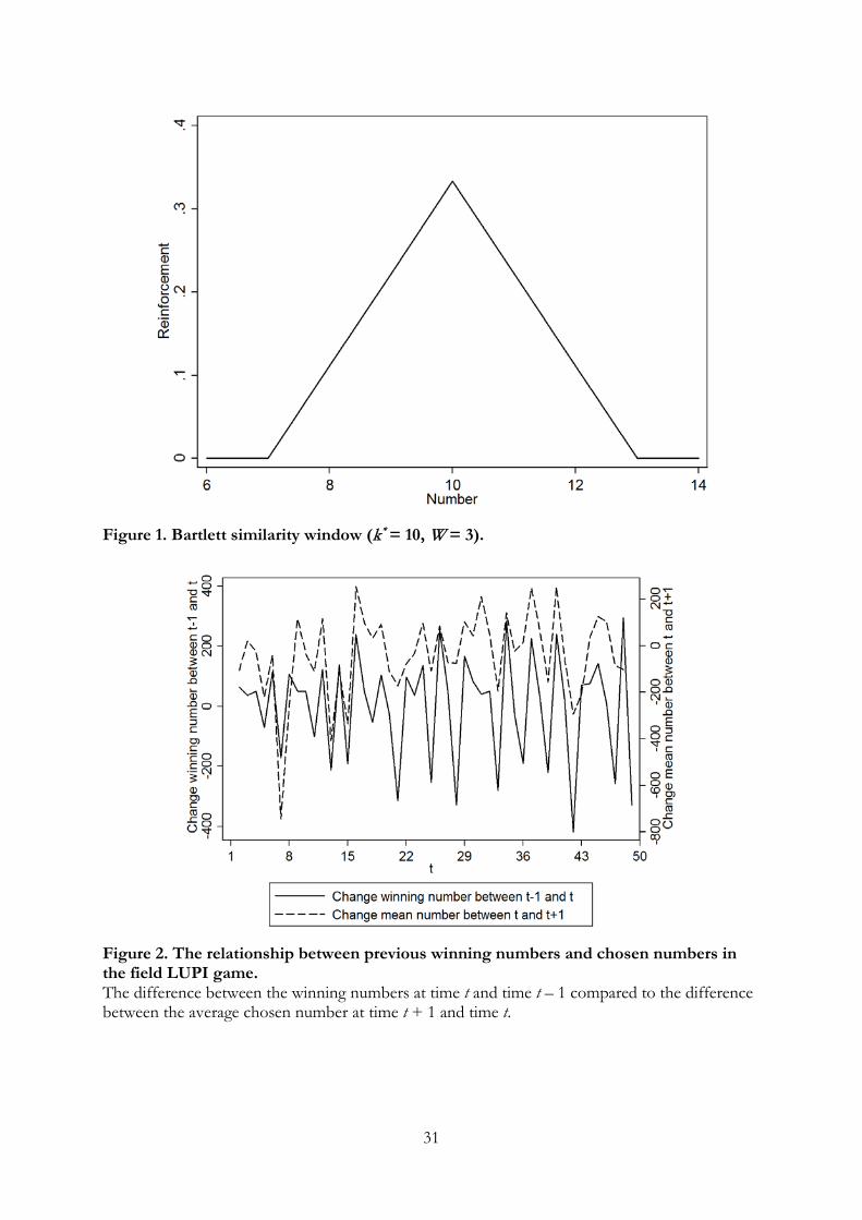
31

Figure 1. Bartlett similarity window (k* = 10, W = 3).

Figure 2. The relationship between previous winning numbers and chosen numbers in the field LUPI game. The difference between the winning numbers at time t and time t – 1 compared to the difference between the average chosen number at time t + 1 and time t.

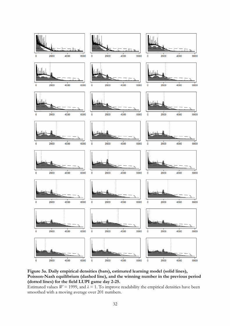
32

Figure 3a. Daily empirical densities (bars), estimated learning model (solid lines), Poisson-Nash equilibrium (dashed line), and the winning number in the previous period (dotted lines) for the field LUPI game day 2-25. Estimated values W = 1999, and λ = 1. To improve readability the empirical densities have been smoothed with a moving average over 201 numbers.

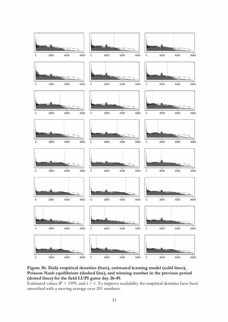
33

Figure 3b. Daily empirical densities (bars), estimated learning model (solid lines), Poisson-Nash equilibrium (dashed line), and winning number in the previous period (dotted lines) for the field LUPI game day 26-49. Estimated values W = 1999, and λ = 1. To improve readability the empirical densities have been smoothed with a moving average over 201 numbers.

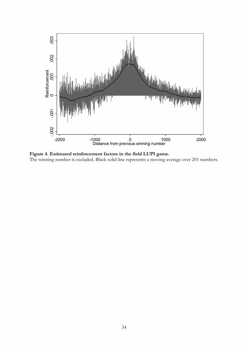
34

Figure 4. Estimated reinforcement factors in the field LUPI game. The winning number is excluded. Black solid line represents a moving average over 201 numbers.

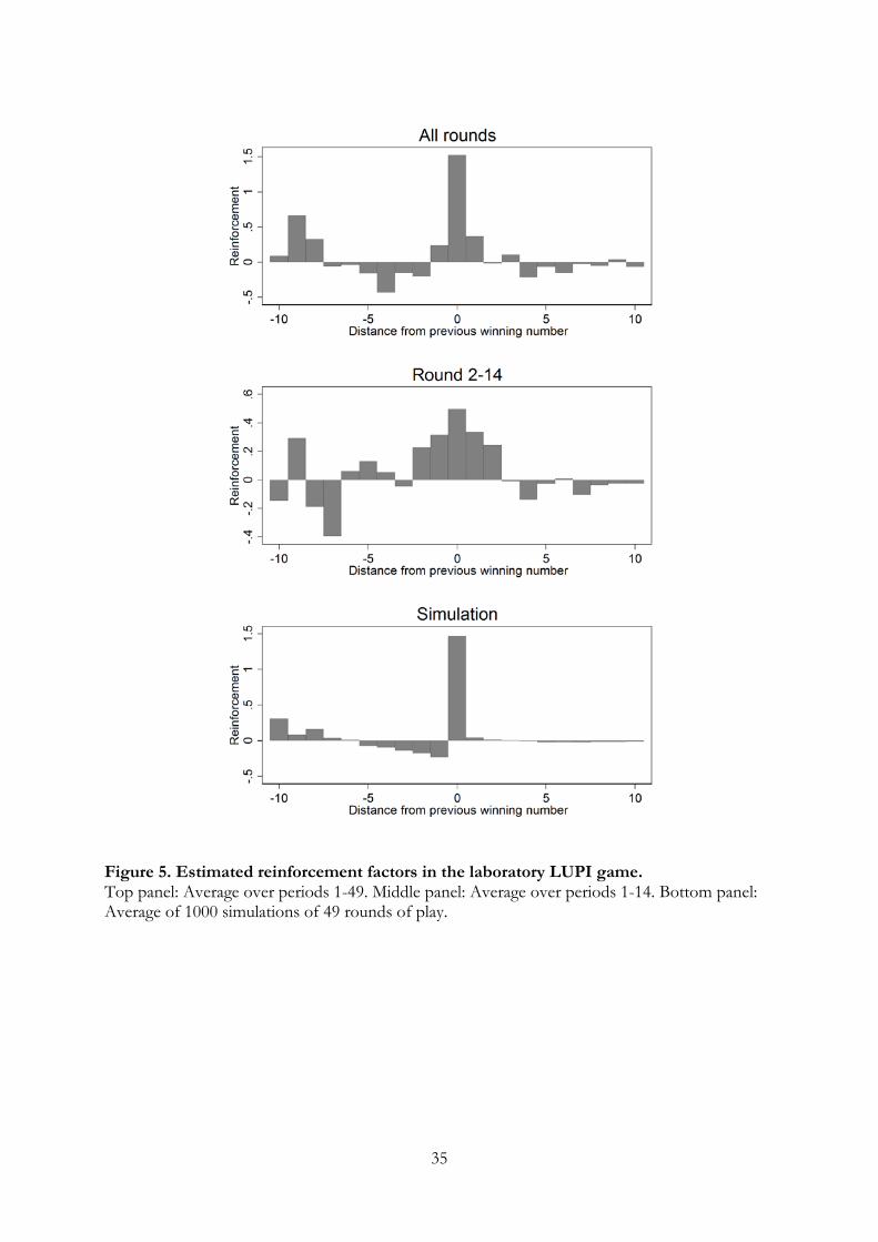
35

Figure 5. Estimated reinforcement factors in the laboratory LUPI game. Top panel: Average over periods 1-49. Middle panel: Average over periods 1-14. Bottom panel: Average of 1000 simulations of 49 rounds of play.

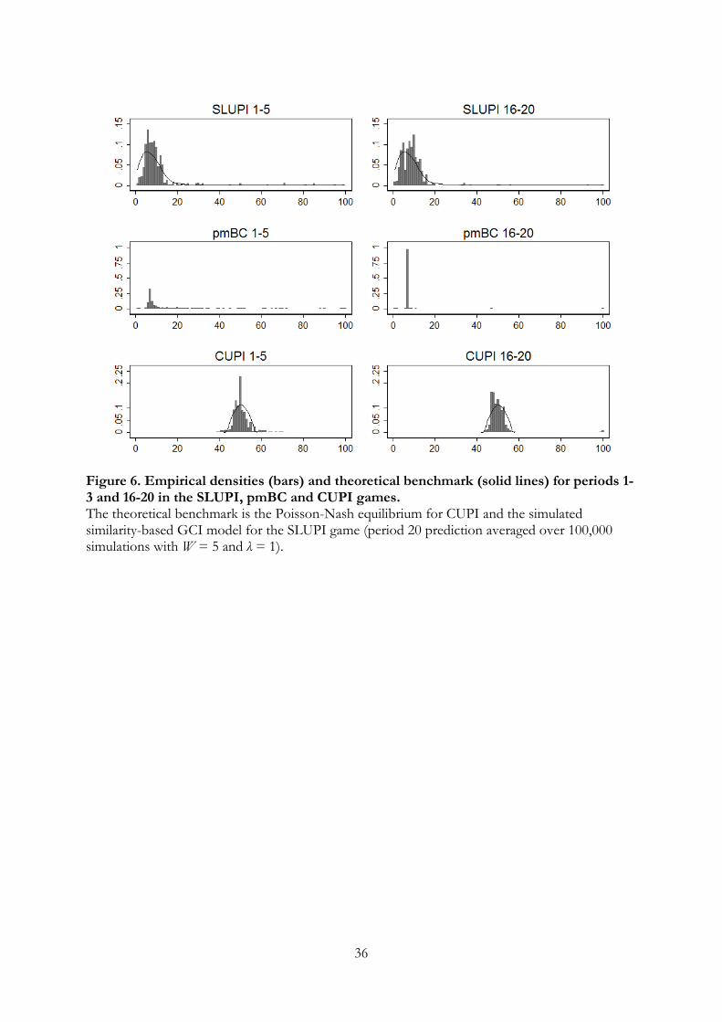
36

Figure 6. Empirical densities (bars) and theoretical benchmark (solid lines) for periods 1-3 and 16-20 in the SLUPI, pmBC and CUPI games. The theoretical benchmark is the Poisson-Nash equilibrium for CUPI and the simulated similarity-based GCI model for the SLUPI game (period 20 prediction averaged over 100,000 simulations with W = 5 and λ = 1).

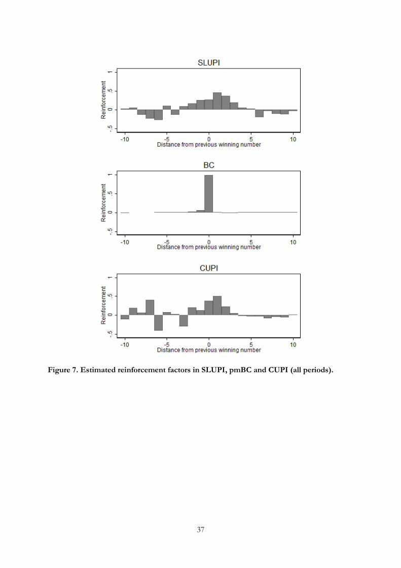
37

Figure 7. Estimated reinforcement factors in SLUPI, pmBC and CUPI (all periods).

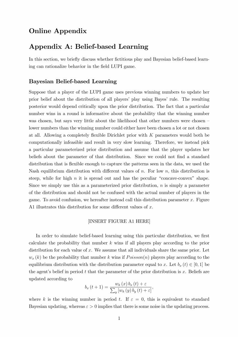
Online Appendix

Appendix A: Belief-based Learning

In this section, we briefly discuss whether fictitious play and Bayesian belief-based learn-

ing can rationalize behavior in the field LUPI game.

Bayesian Belief-based Learning

Suppose that a player of the LUPI game uses previous winning numbers to update her

prior belief about the distribution of all players’play using Bayes’rule. The resulting

posterior would depend critically upon the prior distribution. The fact that a particular

number wins in a round is informative about the probability that the winning number

was chosen, but says very little about the likelihood that other numbers were chosen —

lower numbers than the winning number could either have been chosen a lot or not chosen

at all. Allowing a completely flexible Dirichlet prior with K parameters would both be

computationally infeasible and result in very slow learning. Therefore, we instead pick

a particular parameterized prior distribution and assume that the player updates her

beliefs about the parameter of that distribution. Since we could not find a standard

distribution that is flexible enough to capture the patterns seen in the data, we used the

Nash equilibrium distribution with different values of n. For low n, this distribution is

steep, while for high n it is spread out and has the peculiar “concave-convex” shape.

Since we simply use this as a parameterized prior distribution, n is simply a parameter

of the distribution and should not be confused with the actual number of players in the

game. To avoid confusion, we hereafter instead call this distribution parameter x. Figure

A1 illustrates this distribution for some different values of x.

[INSERT FIGURE A1 HERE]

In order to simulate belief-based learning using this particular distribution, we first

calculate the probability that number k wins if all players play according to the prior

distribution for each value of x. We assume that all individuals share the same prior. Let

wx (k) be the probability that number k wins if Poisson(n) players play according to the

equilibrium distribution with the distribution parameter equal to x. Let bx (t) ∈ [0, 1] be

the agent’s belief in period t that the parameter of the prior distribution is x. Beliefs are

updated according to

bx (t+ 1) =wk (x) bx (t) + ε∑y [wk (y) by (t) + ε]

,

where k is the winning number in period t. If ε = 0, this is equivalent to standard

Bayesian updating, whereas ε > 0 implies that there is some noise in the updating process.

1

This noise term is required to ensure that all probabilities are positive —otherwise some

probabilities will be rounded off to zero.

We have estimated this belief-based learning model for the field data using the ac-

tual winning numbers and setting n = 53, 783 and K = 99, 999. We allowed x ∈1, 2, 3, ..., 99999 and assumed a uniform prior over x, i.e. bx (0) = 1/99999 for all x. We

first set ε to 10−20. Figure A2 shows the value of x that results in the highest value of

wx (k) along with the winning numbers in the field. As is clear from Figure A2, the most

likely x closely follows the winning number. The reason is that the most likely value of

x when k wins is such that the equilibrium distribution “drops”to zero just around k.

The best-response to this distribution would be to play just above k in the next round.

However, belief-learners also take winning numbers from previous rounds into account.

Number 280 wins in the first day, and beliefs in the second day are therefore centered

around x = 1731. The best-response to this belief is to play 281. On the second day,

number 922 wins, which is extremely unlikely if players play according to a distribution

with x = 1731. As shown by Figure A3, the agent therefore starts believing that x is

around 60, 000 from the third day and onwards, i.e. close to the actual number of players

in the field. The reason is that a low number could win either if the distribution happens

to drop at the right place, or when the distribution is very spread out. In the last week,

beliefs are centered around x = 57, 000. Since the agent believes that x is higher than

the number of players, guesses are believed to be more spread out than they actually are

and the best response is to pick 1 from the third round and onwards.

[INSERT FIGURE A2 HERE]

[INSERT FIGURE A3 HERE]

It is clear that belief-based learning with our particular choice of a parameterized

distribution cannot rationalize imitative behavior in the field. Interestingly, however, the

model can rationalize imitative behavior for higher values of the noise parameter. A

high epsilon essentially implies a higher degree of forgetting and, consequently, that the

experience of the last round is relatively more important. For example, if we set ε = 10−10,

the peak of the agent’s posterior corresponds to the most likely x in each period shown

in Figure A2. The best-response to these beliefs is to pick a number slightly above the

previous winning numbers during most of the rounds.

2

Fictitious Play

In our laboratory LUPI experiments, players only observed previous winning numbers.

In the field game, however, it was possible to do so with some effort (by downloading and

processing raw text files from the gambling company’s website). Although we strongly

suspect that not many players did this, we cannot rule it out. We therefore also estimate

a fictitious play learning model in which players form beliefs about which numbers that

will be chosen based on the past empirical distribution, and noisly best respond to those

beliefs.

In this model, the perceived probability that number k is chosen in period t + 1 is

given by

bk (t+ 1) =t∑

s=1

pk (s)

t,

where pk (t) is the empirical frequency with which number k was played in t. For these

beliefs, we calculate the expected payoff of each number assuming that the number of

players are Poission distributed. These expected payoffs are transformed into choice

probabilities using the same power function (3) as in the estimation of the other learning

models. Choices in the first period are assumed be identical to the actual distribution of

play. The resulting model only has one free parameter, the precision parameter λ.

The best-fitting lambda is λ = 0.0036 and the SSD is 0.0075. The fit is considerably

poorer than the imitation learning model which has a SSD of 0.0044 in our baseline

estimation. One caveat is that player heterogeneity might bias estimates in favor of

imitation learning, as discussed by Wilcox (2006). Since we do not have individual-level

data for the field LUPI game, it is diffi cult to correct for this potential bias. Figure

A4 shows the median chosen number in the field together with the predicted median

choice according to the estimated fictitious play and GCI model. Although it is clear

that fictitious play predicts the upward drift in choices in the field data, fictitious play

seems to be too rapid and predicts too high numbers. Figure A5 shows that the fictitious

play model also seems to underpredict the fraction of low numbers that are played —

since numbers below 100 are very common in the data, the expected payoff of playing

low numbers is low, and fictitious play therefore predicts that low numbers are played

with low probability. Although the fit of the fictitious play model might be improved, for

example by assuming that there is a constant inflow of new players with uniform priors,

we believe that ficitious play is a less convincing explanation for several other reasons: 1)

few players probably accessed the complete distribution, 2) calculating expected payoffs

given the empirical distribution is very complicated, and 3) learning in the laboratory is

very rapid despite the fact that only feedback about winning numbers is available.

[INSERT FIGURE A4 HERE]

3

[INSERT FIGURE A5 HERE]

4

Appendix B: Additional Empirical Results

[INSERT FIGURES B1-B10 HERE.]

5

Appendix C: Experimental Instructions

Experimental Payment

At the end of the experiment, you will receive a show-up fee of NT$100, and whatever

amount of Experimental Standard Currency (ESC) you earned in the experiment con-

verted into NT dollars. The amount you will receive, which will be different for each

participant, depends on your decisions, the decisions of others, and chance. All earnings

are paid in private and you are not obligated to tell others how much you have earned.

Note: The exchange rate for Experimental Standard Currency and NT dollars is 1:1 (1

ESC = NT$1).

Note: Please do not talk during the experiment. Raise your hand if you have any

questions; the experimenter will come to you and answer them.

Instructions for Part I

Part I consists of 20 rounds. In each round, everyone has to choose a whole number

between 1 and 100. Whoever chooses the second-lowest, uniquely chosen number wins.

For example, if the chosen numbers are (in order) 1, 1, 1, 2, 3, 3, 4, 5, 5, 5, 6, 7, 7, the

unique numbers are 2, 4, 6. The second lowest among them is 4, so whoever chose 4 is

the winner of this round. If there is no second-lowest unique number, nobody wins this

round.

Raise your hand if you have any questions; the experimenter will come to you and

answer them.

Now we will start Part I and there will be 20 rounds. All of the Experimental Standard

Currency (ESC) you earn in these rounds will be converted into NT dollars according

to the 1:1 exchange rate and given to you. So please chose carefully when making your

decisions.

Instructions for Part II

Part II also consists of 20 rounds. In each round, everyone has to choose a whole number

between 1 and 100. The computer will then calculate the median of all chosen numbers.

Whoever chooses closest to “(median)x0.3+5” wins. For example, if there are three

participants and they choose 1, 2, and 3. The median is 2, and 2x0.3+5=5.6. Among 1,

2, and 3, the closest number to 5.6 is 3, so whoever chose 3 is the winner of this round. If

there are two or more people who choose the closest number, the computer will randomly

choose one of them to be the winner.

Raise your hand if you have any questions; the experimenter will come to you and

answer them.

6

Now we will start Part II and there will be 20 rounds. All of the Experimental

Standard Currency (ESC) you earn in these rounds will be converted into NT dollars

according to the 1:1 exchange rate and given to you. So please chose carefully when

making your decisions.

Instructions for Part III

Part III consists of 20 rounds. In each round, everyone has to choose a whole number

between 1 and 100. Whoever chooses closest to 50, uniquely chosen number wins. If

there are two numbers of the same distance to 50, the larger number wins. For example,

you win if there are two or more who choose 50 and you uniquely choose 51. If there are

two or more who choose 50 and 51, we will have to check (in order) if anyone uniquely

chose 49, 52, 48, etc.

[INSERT FIGURE C1 HERE]

If no number is uniquely chosen, nobody wins in this round.

Raise your hand if you have any questions; the experimenter will come to you and

answer them.

Now we will start Part III and there will be 20 rounds. All of the Experimental

Standard Currency (ESC) you earn in these rounds will be converted into NT dollars

according to the 1:1 exchange rate and given to you. So please chose carefully when

making your decisions.

7

Appendix D: Additional Results and Proofs

Probability Matching in LUPI

Proposition D1 shows that, in equilibrium, the probability a number is played is propor-

tional to the probability that number wins. The probability that number k wins in the

LUPI game is wk (p) = Npkπk (p), where N can be either fixed or Poisson-distributed.

Proposition D1 Consider the LUPI game and suppose that p has full support. Thereis probability matching, pk = wk/

∑j wj for all k, if and only if p is the symmetric Nash

equilibrium.

Proof. Suppose that p is the symmetric Nash equilibrium. Since p has full supportπk = π∗ for all k we have

wk = Npkπ∗. (D1)

Summing both sides of (D1) over k gives∑wk = Nπ∗

∑pk = Nπ∗.

Dividing the left-hand side of (D1) with∑wk and the right-hand side with Nπ∗ gives

pk = wk/∑wk.

To prove the other direction, suppose that p is a mixed strategy with full support that

satisfies pk = wk/∑

j wj. Since wk = Npkπk we have

pk =Npkπk∑

j wj,

or equivalently πk =∑

j wj/N . Because the right-hand side is the same for all k, it must

be a mixed strategy equilibrium. Q.E.D.

Proof of Proposition 1

We borrow the following notation and definitions from Benaïm (1999), which was already

mentioned in a footnote in the main text: Consider a metric space (X, d) (in our case

it is the simplex ∆ and Euclidean distance) and a semi-flow Φ : R+ × X → X induced

by a vector field F on X. A point x ∈ X is a rest point (an equilibrium in Benaïm’s

terminology) if Φt (x) = x for all t. A point x∗ ∈ X is an ω-limit point of x if x∗ =

limtk→∞Φtk (x) for some sequence tk → ∞. Intuitively, an ω-limit point of x is a pointto which the semi-flow Φt (x) always returns. The ω-limit set of x, denoted ω (x), is the

set of ω-limit points of x. The definition of an ω-limit can be extended to a discrete

time system. A set A ⊆ X is invariant if Φt (A) = A for all t ∈ R. A subset A ⊆ X

is an attractor for Φ if (i) A is non-empty, compact and invariant, and (ii) A has a

8

neighborhood U ⊆ X such that limt→∞ d (Φt, A) → 0 uniformly in x ∈ U (the distance

between Φt and the closest point in A). An attractor A is a proper attractor if it contains

no proper subset that is an attractor.

For δ > 0, and T > 0, a (δ, T )-pseudo-orbit from a ∈ X to b ∈ X is a finite sequence

of partial trajectories Φt (yi) : 0 ≤ t ≤ tii=0,...,k−1, with ti ≥ T , such that d (y0, a) < δ,

d(Φtj (yj) , yj+1

)< δ for j = 0, ..., k − 1, and yk = b. A point a ∈ X is chain recurrent if

there is a (δ, T )-pseudo-orbit from a to a for every δ > 0, and T > 0. Let Λ ⊆ X be a

non-empty invariant set. Φ is called chain recurrent on Λ if every point x ∈ Λ is a chain

recurrent point for Φ|Λ, the restriction of Φ to Λ. A compact invariant set on which Φ

is chain recurrent is called an internally chain recurrent set. Armed with these concepts,

we may prove Proposition 1.

We being by deriving an expressions for the law of motion of p (t).

pk (t+ 1)− pk (t) =Ak (t+ 1)∑Kj=1Aj (t+ 1)

− Ak (t)∑Kj=1Aj (t)

=Ak (t) + rk (t)∑K

j=1 (Aj (t) + rj (t))− pk (t)

=Ak (t) + rk (t)− pk (t)

∑Kj=1 (Aj (t) + rj (t))∑K

j=1 (Aj (t) + rj (t))

=rk (t)− pk (t)

∑Kj=1 rj (t)∑K

j=1Aj (t+ 1). (D2)

This formulation makes it clear that p (t) is a process with decreasing step size since c > 0

ensures that the sum of reinforcements grows without bound. Note that the stochastic

nature of the process is due to randomness of the reinforcement terms rj (t)Kj=1, whichalso enter into

∑Kj=1Aj (t+ 1), by the definition of the updating rule (2).

Let (Ω,F , µ) be a probability space and Ft a filtration such that Ft is a sigma-algebra that represents the history of the system up until the beginning of period t. The

process p is adapted to Ft. We can write

p (t+ 1)− p (t) = γ (t+ 1) (F (t) + U (t+ 1)) ,

where the step size is

γ (t+ 1) =1∑K

j=1Aj (t+ 1),

the expected motion is

F (t) = E [rk (t) |Ft]− pk (t)

K∑j=1

E [rj (t) |Ft] ,

9

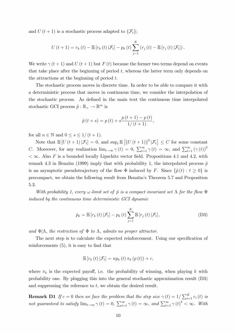
and U (t+ 1) is a stochastic process adapted to Ft;

U (t+ 1) = rk (t)− E [rk (t) |Ft]− pk (t)K∑j=1

(rj (t)− E [rj (t) |Ft]) .

We write γ (t+ 1) and U (t+ 1) but F (t) because the former two terms depend on events

that take place after the beginning of period t, whereas the latter term only depends on

the attractions at the beginning of period t.

The stochastic process moves in discrete time. In order to be able to compare it with

a deterministic process that moves in continuous time, we consider the interpolation of

the stochastic process. As defined in the main text the continuous time interpolated

stochastic GCI process p : R+ → Rm is

p (t+ s) = p (t) + sp (t+ 1)− p (t)

1/ (t+ 1),

for all n ∈ N and 0 ≤ s ≤ 1/ (t+ 1).

Note that E [U (t+ 1) |Ft] = 0, and supt E[‖U (t+ 1)‖2 |Ft

]≤ C for some constant

C. Moreover, for any realization limt→∞ γ (t) = 0,∑∞

t=1 γ (t) = ∞, and∑∞

t=1 (γ (t))2

< ∞. Also F is a bounded locally Lipschitz vector field. Propositions 4.1 and 4.2, with

remark 4.3 in Benaïm (1999) imply that with probability 1, the interpolated process p

is an asymptotic pseudotrajectory of the flow Φ induced by F . Since p (t) : t ≥ 0 isprecompact, we obtain the following result from Benaïm’s Theorem 5.7 and Proposition

5.3.

With probability 1, every ω-limit set of p is a compact invariant set Λ for the flow Φ

induced by the continuous time deterministic GCI dynamic

pk = E [rk (t) |Ft]− pk (t)K∑j=1

E [rj (t) |Ft] , (D3)

and Φ|Λ, the restriction of Φ to Λ, admits no proper attractor.

The next step is to calculate the expected reinforcement. Using our specification of

reinforcements (5), it is easy to find that

E [rk (t) |Ft] = npk (t) πk (p (t)) + c,

where πk is the expected payoff, i.e. the probability of winning, when playing k with

probability one. By plugging this into the general stochastic approximation result (D3)

and suppressing the reference to t, we obtain the desired result.

Remark D1 If c = 0 then we face the problem that the step size γ (t) = 1/∑K

i=1 ri (t) is

not guaranteed to satisfy limt→∞ γ (t) = 0,∑∞

t=1 γ (t) = ∞, and∑∞

t=1 γ (t)2 < ∞. With

10

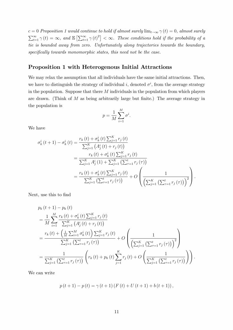
c = 0 Proposition 1 would continue to hold if almost surely limt→∞ γ (t) = 0, almost surely∑∞t=1 γ (t) = ∞, and E

[∑∞t=1 γ (t)2

]< ∞. These conditions hold if the probability of a

tie is bounded away from zero. Unfortunately along trajectories towards the boundary,

specifically towards monomorphic states, this need not be the case.

Proposition 1 with Heterogenous Initial Attractions

We may relax the assumption that all individuals have the same initial attractions. Then,

we have to distinguish the strategy of individual i, denoted σi, from the average strategy

in the population. Suppose that thereM individuals in the population from which players

are drawn. (Think of M as being arbitrarily large but finite.) The average strategy in

the population is

p =1

M

M∑i=1

σi.

We have

σik (t+ 1)− σik (t) =rk (t) + σik (t)

∑Kj=1 rj (t)∑K

j=1

(Aij (t) + rj (t)

)=

rk (t) + σik (t)∑K

j=1 rj (t)∑Kj=1A

ij (1) +

∑Kj=1

(∑tτ=1 rj (τ)

)=rk (t) + σik (t)

∑Kj=1 rj (t)∑K

j=1

(∑tτ=1 rj (τ)

) +O

1(∑Kj=1

(∑tτ=1 rj (τ)

))2 .

Next, use this to find

pk (t+ 1)− pk (t)

=1

M

M∑i=1

rk (t) + σik (t)∑K

j=1 rj (t)∑Kj=1

(Aij (t) + rj (t)

)=rk (t) +

(1M

∑Mi=1 σ

ik (t)

)∑Kj=1 rj (t)∑K

j=1

(∑tτ=1 rj (τ)

) +O

1(∑Kj=1

(∑tτ=1 rj (τ)

))2

=1∑K

j=1

(∑tτ=1 rj (τ)

) (rk (t) + pk (t)K∑j=1

rj (t) +O

(1∑K

j=1

(∑tτ=1 rj (τ)

))) .We can write

p (t+ 1)− p (t) = γ (t+ 1) (F (t) + U (t+ 1) + b (t+ 1)) ,

11

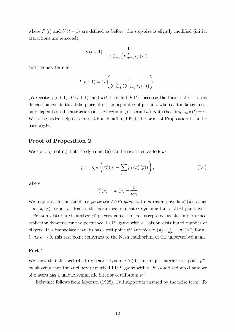
where F (t) and U (t+ 1) are defined as before, the step size is slightly modified (initial

attractions are removed),

γ (t+ 1) =1∑K

j=1

(∑tτ=1 rj (τ)

) ,and the new term is -

b (t+ 1) = O

(1∑K

j=1

(∑tτ=1 rj (τ)

)) .(We write γ (t+ 1), U (t+ 1), and b (t+ 1), but F (t), because the former three terms

depend on events that take place after the beginning of period t whereas the latter term

only depends on the attractions at the beginning of period t.) Note that limt→∞ b (t) = 0.

With the added help of remark 4.5 in Benaïm (1999), the proof of Proposition 1 can be

used again.

Proof of Proposition 2

We start by noting that the dynamic (6) can be rewritten as follows

pk = npk

(πck (p)−

K∑j=1

pj(πcj (p)

)), (D4)

where

πci (p) = πi (p) +c

npi.

We may consider an auxiliary perturbed LUPI game with expected payoffs πci (p) rather

than πi (p) for all i. Hence, the perturbed replicator dynamic for a LUPI game with

a Poisson distributed number of players game can be interpreted as the unperturbed

replicator dynamic for the perturbed LUPI game with a Poisson distributed number of

players. It is immediate that (6) has a rest point pc∗ at which πi (p)+ cnpi

= πi (pc∗) for all

i. As c→ 0, this rest point converges to the Nash equilibrium of the unperturbed game.

Part 1

We show that the perturbed replicator dynamic (6) has a unique interior rest point pc∗,

by showing that the auxiliary perturbed LUPI game with a Poisson distributed number

of players has a unique symmetric interior equilibrium pc∗.

Existence follows from Myerson (1998). Full support is ensured by the noise term. To

12

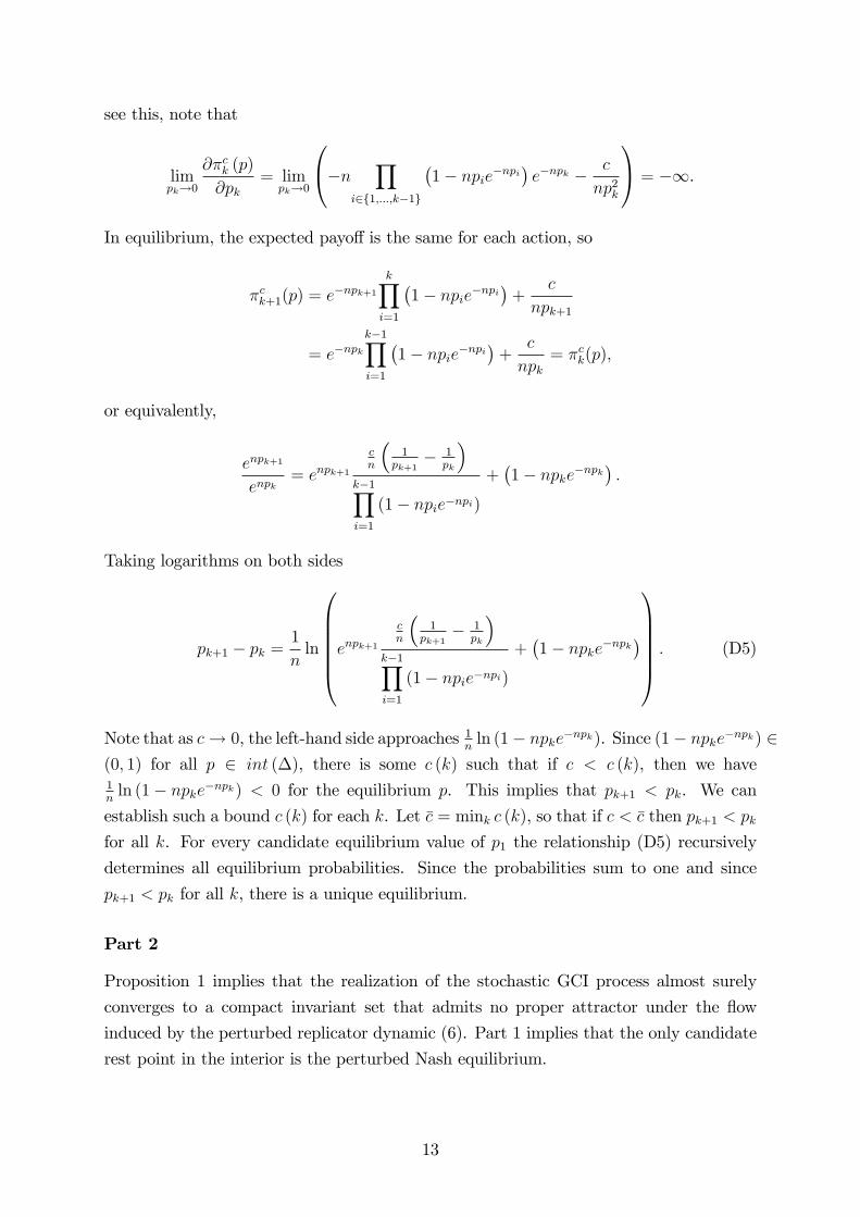
see this, note that

limpk→0

∂πck (p)

∂pk= lim

pk→0

−n ∏i∈1,...,k−1

(1− npie−npi

)e−npk − c

np2k

= −∞.

In equilibrium, the expected payoff is the same for each action, so

πck+1(p) = e−npk+1k∏i=1

(1− npie−npi

)+

c

npk+1

= e−npkk−1∏i=1

(1− npie−npi

)+

c

npk= πck(p),

or equivalently,

enpk+1

enpk= enpk+1

cn

(1

pk+1− 1

pk

)k−1∏i=1

(1− npie−npi)+(1− npke−npk

).

Taking logarithms on both sides

pk+1 − pk =1

nln

enpk+1cn

(1

pk+1− 1

pk

)k−1∏i=1

(1− npie−npi)+(1− npke−npk

) . (D5)

Note that as c→ 0, the left-hand side approaches 1n

ln (1− npke−npk). Since (1− npke−npk) ∈(0, 1) for all p ∈ int (∆), there is some c (k) such that if c < c (k), then we have1n

ln (1− npke−npk) < 0 for the equilibrium p. This implies that pk+1 < pk. We can

establish such a bound c (k) for each k. Let c = mink c (k), so that if c < c then pk+1 < pk

for all k. For every candidate equilibrium value of p1 the relationship (D5) recursively

determines all equilibrium probabilities. Since the probabilities sum to one and since

pk+1 < pk for all k, there is a unique equilibrium.

Part 2

Proposition 1 implies that the realization of the stochastic GCI process almost surely

converges to a compact invariant set that admits no proper attractor under the flow

induced by the perturbed replicator dynamic (6). Part 1 implies that the only candidate

rest point in the interior is the perturbed Nash equilibrium.

13

Part 3

To rule out convergence to the boundary, recall that the initial attractions are strictly

positive. Since no boundary point is a Nash equilibrium, the proofs of Lemma 3 and

Proposition 3 in Hopkins and Posch (2005) can be adapted; for instance one may consider

the unperturbed dynamic in the perturbed game (defined by the perturbed payoffs πc).

If p′ 6= pc∗, then p′ is not a Nash equilibrium of the perturbed game. If a point p′ is not

a Nash equilibrium, then the Jacobian for the replicator dynamic, evaluated at p′, has at

least one strictly positive eigenvalue. Hopkins and Posch (2005) show that this rules out

convergence. For a related point, see Beggs (2005).

14

Appendix E: A Family of GCI Models

In order to be able to generalize the learning rule that we defined for LUPI, we define four

different versions of GCI that happen to coincide in LUPI and winner-takes-all games,

but which may yield different predictions in other games. Therefore, we make two fur-

ther distinctions. First, imitation may or may not be responsive to the number of people

who play different strategies. This leads us to distinguish frequency-dependent (FD) and

frequency-independent (FI) versions of GCI. The interaction between payoffs and frequen-

cies may take many forms, but, for simplicity, we assume a multiplicative interaction, i.e.

reinforcement in the frequency-dependent model depends on the total payoff of all play-

ers that picked an action. Second, imitation may be exclusively focused on emulating

the winning action, i.e. the action that obtained the highest payoff, or be responsive to

payoff-differences in a proportional way. Thus, we differentiate between winner—takes-all

imitation (W) and payoff-proportional imitation (P). In total we introduce the following

four members of the GCI family: PFI, PFD, WFD, and WFI.

Under payoff-proportional frequency-independent global cumulative imitation (PFI-

GCI), reinforcements are

rPFIk (t) =

usi(t) (s (t)) + c if si (t) = k for some i,

c otherwise.(E1)

Such reinforcements can be calculated based only on information about the payoff that

was received by actions that someone played. Alternatively, players may also have infor-

mation about the number of players playing each strategy. Let mk (t) be the number of

players picking k at time t. This information is utilized by reinforcement under payoff-

proportional frequency-dependent global cumulative imitation (PFD-GCI),

rPFDk (t) =

mk (t)

(usi(t) (s (t)) + c

)if si (t) = k for some i,

mk (t) c otherwise.(E2)

In the LUPI experiments, subjects do not have any information about mk (t) unless

k is the winning number. However, if c = 0 then mk (t) c = 0 so that rPFDk (t) = 0 for

all k other than the winning number. Thus, for c = 0 subjects in our LUPI experiments

could update attractions with reinforcements of the form rPFDk (t).

Next consider imitation that only reinforces the winning actions —the highest earning

action. In line with Roth (1995), we define winner-takes-all frequency-independent global

cumulative imitation (WFD-GCI),

rWFIk (t) =

usi(t) (s (t)) + c if si (t) = k ∈ maxsi(t) u (si (t) , s−i (t)) ,

0 otherwise.(E3)

15

Roth does not explicitly add a constant c but he assumes, equivalently, that all payoffs

are strictly positive.

We also define a frequency-dependent version of winner-takes-all imitation (which is

not mentioned in Roth, 1995); winner-takes-all frequency-dependent global cumulative

imitation (WFI-GCI),

rWFDk (t) =

mk (t)

(usi(t) (s (t)) + c

)if si (t) = k ∈ maxsi(t) u (si (t) , s−i (t)) ,

0 otherwise.(E4)

As in the case of rPFD, if c = 0, thenmk (t) c = 0 so that rWFDk (t) = 0 for all k other than

the winning number. Thus, for c = 0, subjects in our LUPI experiments could update

attractions with reinforcements of the form rWFDk (t).

The following proposition relates the four different members of the GCI family in

winner-takes-all games.

Proposition E1 In winner-takes-all games

limc→0

rPFIk (t) = limc→0

rPFDk (t) limc→0

= rWFIk (t) lim

c→0= rWFD

k (t) =

1 if k = k∗ (s (t))

0 otherwise..

Proof. Follows from the fact that in winner-takes-all games, mk (t)uk (s (t)) = 1 for

winning k and u (k, s−i) = 0 for losing k. Q.E.D.

Proposition E1 means that we are unable to distinguish the members of the GCI

family in winner-takes-all games. However, in general, the different members of the GCI-

family can be distinguished as they induce different dynamics. We can show that PFD

induces a noisy replicator dynamic in all games.

Proposition E2 Consider a symmetric game and assume that c > mins∈S ui (si, s−i).

In a fixed N-player game, the GCI continuous time dynamic with PFD-reinforcement

(E2) is

pk = Npk

(πk (p)−

K∑j=1

pjπj (p)

)+ c (1−Kpk) .

In a Poisson n-player game, the GCI continuous time dynamic with PFD-reinforcement

(E2) is

pk = npk

(πk (p)−

K∑j=1

pjπj (p)

)+ c (1−Kpk) .

Proof. Let Xt (k) be the total number of players who are drawn to participate and

choose strategy k in period t. For a given focal individual who is drawn to play the

game, let Yt (k) be the number of other players who pick k in period t. In the Poisson

game, the ex ante probability of Xt(k) = m is equal to the probability that Yt(k) = m

16

conditional on the focal individual being drawn to play. This is due to the environmental

equivalence-property of Poisson games (Myerson, 1998). However in a game with a fixed

number of N players, this is not the case.

We now derive the expected reinforcement ρPFD. To simplify the exposition, we

suppress the reference to Ft. For both fixed and Poisson distributed number of players,we have

E[rPFDk (t) |Ft

]=

N∑j=1

Pr (X (k) = j)E[rPFDk (s) |X (k) = j

]+ Pr (X (k) = 0) (c · 0)

=

N∑j=1

Pr (X (k) = j)E [j · (uk (s (t)) + c) |Y (k) = j − 1 ∧X (k) = j]

=N−1∑j=0

Pr (X (k) = j + 1)E [(j + 1) (uk (s (t)) + c) |Y (k) = j ∧X (k) = j + 1] . (E5)

For fixed N-player games, we need to translate from Pr (X (k) = j + 1) to Pr (Y (k) = j).

Use

Pr (Y (k) = j) =

(N − 1

j

)pjk (1− pk)N−1−j

=(n− 1)!

j! (n− 1− j)!pjk (1− pk)N−1−j ,

to obtain

Pr (X (k) = j + 1) =

(N

j + 1

)pj+1k (1− pk)N−(j+1)

=N !

(j + 1)! (N − (j + 1))!pj+1k (1− pk)N−j−1

=Npkj + 1

(N − 1)!

j! (N − j − 1)!pjk (1− pk)N−j−1

=Npkj + 1

Pr (Yi (k) = j) .

Plugging this into (E5) yields

E[rPFDk (t) |Ft

]=

N−1∑j=0

Npkj + 1

Pr (Yi (k) = j)E [(j + 1) (uk (s (t)) + c) |Y (k) = j ∧X (k) = j + 1]

= Npk

N−1∑j=0

Pr (Yi (k) = j)E [(uk (s (t)) + c) |Y (k) = j ∧X (k) = j + 1] ,

17

or

E[rPFDk (t) |Ft

]= Npk (πk (p (t)) + c) . (E6)

Plugging (E6) into the general stochastic approximation result (D3) gives the desired

result for fixed N -player games.

For Poisson-distributed N , we have

Pr (X (k) = j + 1) =enpk (npk)

j+1

(j + 1)!=

npkj + 1

enpk (npk)j

j!=

npkj + 1

Pr (X (k) = j + 1) .

Plugging this into (E5) yields

E[rPFDk (t) |Ft

]=

N−1∑j=0

npkj + 1

Pr (X (k) = j + 1)E [(j + 1) (uk (s (t)) + c) |Y (k) = j ∧X (k) = j + 1]

= npk

N−1∑j=0

Pr (X (k) = j + 1)E [(uk (s (t)) + c) |Y (k) = j ∧X (k) = j + 1]

= npk (πk (p (t)) + c) .

Using this in the general stochastic approximation result (D3) gives the desired result for

Poisson games. Q.E.D.

The other three GCI models —PFI, WFI and WFD —do not generally lead to any

version of the replicator dynamic. This can be verified by calculating the expected rein-

forcement and plugging it into equation (D3). The different models also differ in their

informational requirements: WDI requires the least feedback, whereas PFD requires the

most. Nevertheless, players could still use all four models in our experimental games

although they only receive feedback about the action that obtained the highest payoff,

i.e. the winner. Since players can infer the payoff of all other players (zero unless they

win), they can use both winner-imitation and proportional imitation. Moreover, even

though they only know the number of individuals who picked the winning action (one

individual), they are still able to compute the product of payoffand the number of players

for all actions (since it is zero for all non-winning actions). For this reason, they are able

to use both frequency dependent and frequency independent imitation.

18

Similarity-weighted GCI in LUPI

We may add similarity-weights to each of the specifications of reinforcement defined

above. With the the similarity function (4) reinforcement factors in the LUPI game are

rk (t) =

ηk (k∗ (t)) + c if there is a winner, k∗ (t) , in period t,

c otherwise.. (E7)

Proposition E3 In a LUPI game with a Poisson distributed number of players, the GCIcontinuous time dynamic with reinforcement (E7) is the following dynamic

pk = n

(πk (p)− pk

K∑j=1

πj (p)

)+ (1−K) c, (E8)

where πk denotes the similarity- and frequency-weighted payoff

πk (p) =K∑l=0

plπl (p) ηk (l) .

Proof. Expected reinforcement (E7) is

E [rk (t) |Ft] = E [ηk (k∗ (s (t))) |Ft] + c

= E

max

0, 1− |k∗(s(t))−k|W

∑K

i=0 max

0, 1− |k∗(s(t))−i|W

∣∣∣∣∣∣Ft+ c

=K∑l=0

Pr (k∗ (s (t)) = l|Ft)

max

0, 1− |l−k|W

∑K

i=0 max

0, 1− |l−i|W

+ c

=K∑l=0

npl (t) πl (p (t)) ηk (l) + c.

By using the expression for E [rk (t) |Ft] in the general stochastic approximation result(D3) and suppressing the reference to t, we obtain the desired result. Q.E.D.

Note that this is not the noisy replicator dynamic, hence we cannot be sure that the

limiting behaviour of (E8) is the same as that of (6). A rest point p of (E8) solves, for

each k,

pk =nπk (p) + c

n∑K

j=1 πj (p) +Kc.

19

We can verify that p∗ (the equilibrium of the game without similarity-adjustment) is not

a rest point (when c = 0):

πk (p∗)∑Kj=1 πj (p∗)

=

∑Kl=0 np

∗l πl (p

∗) ηk (l)∑Kl=0 np

∗l πl (p

∗)

=

∑Kl=0 np

∗l π∗ηk (l)∑K

l=0 np∗l π∗

=

∑Kl=0 p

∗l ηk (l)∑K

l=0 p∗l

=K∑l=0

p∗l ηk (l)

6= p∗k.

Figure E1 shows the results from the simulations of similarity-weighted GCI described

in section 5.4.

[INSERT FIGURE E1 HERE]

We study similarity-weighted GCI in the general case by restricting attention to payoff-

proportional, frequency-dependent GCI:

rPFDk (t) =K∑l=1

ηk (l) rPFDl (t) =

∑Kl=1 ηk (l)ml (t)

(usi(t) (s (t)) + c

)if si (t) = k for some i,∑K

l=1 ηk (l)mk (t) c otherwise.(E9)

For this kind of reinforcement the deterministic dynamic is a replicator dynamic for

similarity- and frequency-weighted payoffs, plus a noise term.

Proposition E4 Consider a symmetric game with an ordered strategy set S = 1, 2, ..., Kfor each player. Assume that c > mins∈S u (si, s−i). In a fixed N-player game, the GCI

continuous time dynamic with similarity-weighted PFD-reinforcement (E9) is

pk = N

(πk (p)− pk (t)

K∑j=1

πj (p)

)+ cN

(K∑l=1

plηk (l)− pk (t)

).

In a Poisson n-player game, the GCI continuous time dynamic with PFD-reinforcement

(E2) is

pk = n

(πk (p)− pk (t)

K∑j=1

πj (p)

)+ cn

(K∑l=1

plηk (l)− pk (t)

).

20

As in the main text πk denotes the similarity- and frequency-weighted payoff

πk (p) =K∑l=0

plπl (p) ηk (l) .

Proof. In the Poisson case expected reinforcement is,

E[rPFDk (t) |Ft

]=

K∑l=1

ηk (l)E[rPFDl (t) |Ft

].

=

K∑l=1

ηk (l)npl (πl (p (t)) + c)

=

(K∑l=1

ηk (l)nplπl (p (t)) +

K∑l=1

ηk (l)nplc

)

= n

(πk (p) + c

K∑l=1

ηk (l) pl

)

Using this in (D3) yields

pk = n

(πk (p) + c

K∑l=1

ηk (l) pl

)− npk (t)

K∑j=1

(πj (p) + c

K∑l=1

ηj (l) pl

)

= n

(πk (p)− pk (t)

K∑j=1

πj (p)

)+ cn

K∑l=1

(ηk (l) pl − pk (t) pl)

= n

(πk (p)− pk (t)

K∑j=1

πj (p)

)+ cn

(K∑l=1

plηk (l)− pk (t)

),

A similar result is obtained for the fixed N case. Q.E.D.

21

Appendix F: Global Convergence and Local Stability

Global Convergence

In the main text it is established that if the stochastic GCI-process converges to a point

then it must converge to (a perturbed version of) the unique interior equilibrium. In order

to establish that the process does indeed converge to this point and not to something else

than a point —e.g. a periodic orbit —we simulated the learning process. As explained in

Section 5.2 we used the lab parameters K = 99 and n = 26.9, and randomly drew 100

different initial conditions. For each initial condition, we ran the process for 10 million

rounds. Figure F1 shows the resulting distribution at the end of these 10 million rounds,

averaged over the 100 initial conditions.

[INSERT FIGURE F1 HERE]

Local Stability

Having demonstrated global convergence numerically, the remainder of this Appendix

explores the local stability properties of the unique Nash equilibrium, using a combination

of analytical and numerical methods.

Analytical Methods

Local stability can be determined by studying the Jacobian Dπ (p), where π (p) =

(π1 (p) , ..., πK (p))′ is the column vector of payoffs when the population average strat-

egy is p. A suffi cient condition for the interior equilibrium p∗ to asymptotically stable

under the replicator dynamic is that p∗ is an evolutionarily stable strategy (see e.g. Sand-

holm (2011), theorem 8.4.1). Since p∗ is completely mixed it is an ESS if and only if

its associated Jacobian, Dπ (p∗), is negative definite with respect to the tangent space

(see e.g. Sandholm (2011), theorem 8.3.11). With K strategies, the tangent space is

RK0 = v ∈ RK :∑

i vi = 0 so an interior equilibrium is asymptotically stable if

v′Dπ (p∗) v < 0 for all v ∈ RK0 , v 6= 0.

We will first prove stability in the unperturbed case and then use a continuity argu-

ment to prove stability under the perturbed replicator dynamic.

22

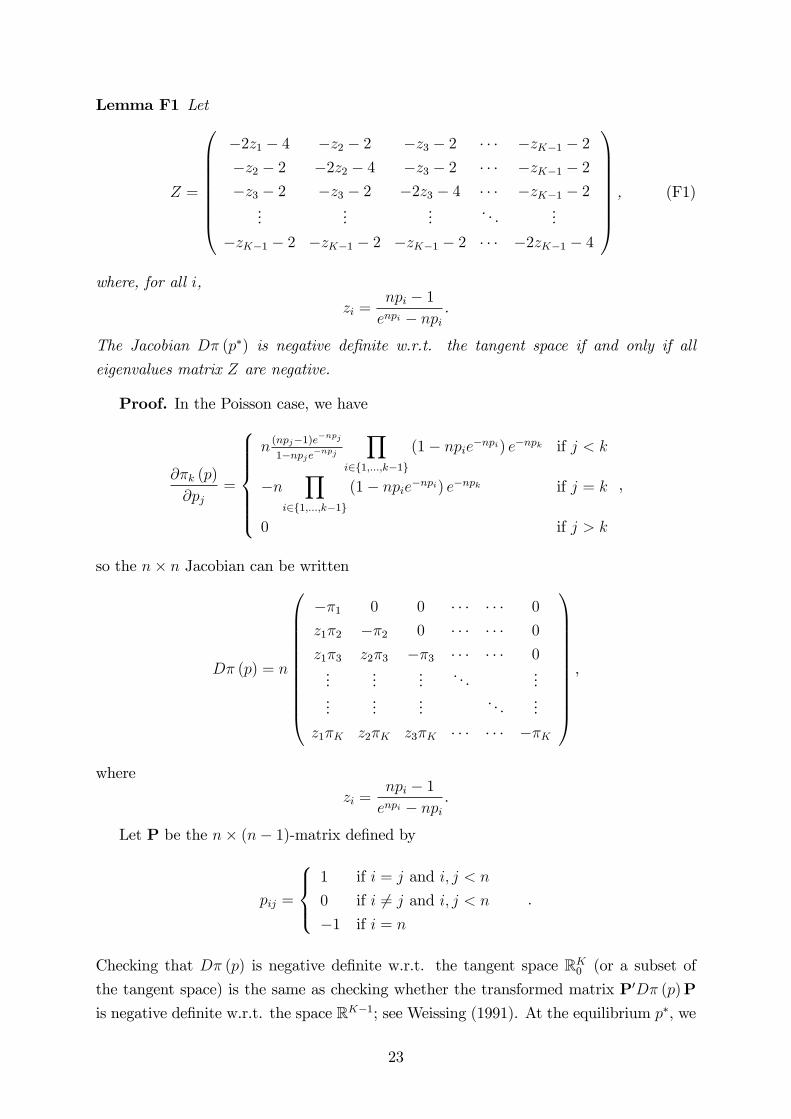
Lemma F1 Let

Z =

−2z1 − 4 −z2 − 2 −z3 − 2 · · · −zK−1 − 2

−z2 − 2 −2z2 − 4 −z3 − 2 · · · −zK−1 − 2

−z3 − 2 −z3 − 2 −2z3 − 4 · · · −zK−1 − 2...

......

. . ....

−zK−1 − 2 −zK−1 − 2 −zK−1 − 2 · · · −2zK−1 − 4

, (F1)

where, for all i,

zi =npi − 1

enpi − npi.

The Jacobian Dπ (p∗) is negative definite w.r.t. the tangent space if and only if all

eigenvalues matrix Z are negative.

Proof. In the Poisson case, we have

∂πk (p)

∂pj=

n(npj−1)e−npj1−npje−npj

∏i∈1,...,k−1

(1− npie−npi) e−npk if j < k

−n∏

i∈1,...,k−1

(1− npie−npi) e−npk if j = k

0 if j > k

,

so the n× n Jacobian can be written

Dπ (p) = n

−π1 0 0 · · · · · · 0

z1π2 −π2 0 · · · · · · 0

z1π3 z2π3 −π3 · · · · · · 0...

......

. . ....

......

.... . .

...

z1πK z2πK z3πK · · · · · · −πK

,

where

zi =npi − 1

enpi − npi.

Let P be the n× (n− 1)-matrix defined by

pij =

1 if i = j and i, j < n

0 if i 6= j and i, j < n

−1 if i = n

.

Checking that Dπ (p) is negative definite w.r.t. the tangent space RK0 (or a subset of

the tangent space) is the same as checking whether the transformed matrix P′Dπ (p)P

is negative definite w.r.t. the space RK−1; see Weissing (1991). At the equilibrium p∗, we

23

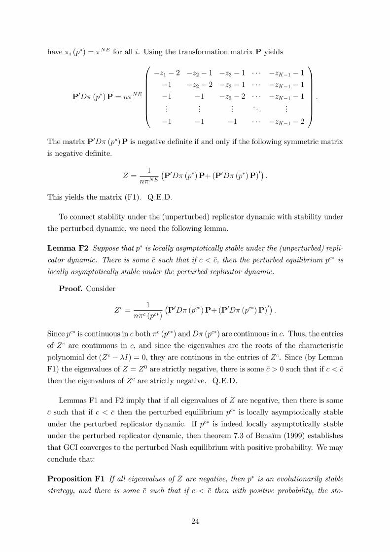
have πi (p∗) = πNE for all i. Using the transformation matrix P yields

P′Dπ (p∗)P = nπNE

−z1 − 2 −z2 − 1 −z3 − 1 · · · −zK−1 − 1

−1 −z2 − 2 −z3 − 1 · · · −zK−1 − 1

−1 −1 −z3 − 2 · · · −zK−1 − 1...

......

. . ....

−1 −1 −1 · · · −zK−1 − 2

.

The matrix P′Dπ (p∗)P is negative definite if and only if the following symmetric matrix

is negative definite.

Z =1

nπNE(P′Dπ (p∗)P+ (P′Dπ (p∗)P)

′) .This yields the matrix (F1). Q.E.D.

To connect stability under the (unperturbed) replicator dynamic with stability under

the perturbed dynamic, we need the following lemma.

Lemma F2 Suppose that p∗ is locally asymptotically stable under the (unperturbed) repli-cator dynamic. There is some c such that if c < c, then the perturbed equilibrium pc∗ is

locally asymptotically stable under the perturbed replicator dynamic.

Proof. Consider

Zc =1

nπc (pc∗)

(P′Dπ (pc∗)P+ (P′Dπ (pc∗)P)

′) .Since pc∗ is continuous in c both πc (pc∗) andDπ (pc∗) are continuous in c. Thus, the entries

of Zc are continuous in c, and since the eigenvalues are the roots of the characteristic

polynomial det (Zc − λI) = 0, they are continous in the entries of Zc. Since (by Lemma

F1) the eigenvalues of Z = Z0 are strictly negative, there is some c > 0 such that if c < c

then the eigenvalues of Zc are strictly negative. Q.E.D.

Lemmas F1 and F2 imply that if all eigenvalues of Z are negative, then there is some

c such that if c < c then the perturbed equilibrium pc∗ is locally asymptotically stable

under the perturbed replicator dynamic. If pc∗ is indeed locally asymptotically stable

under the perturbed replicator dynamic, then theorem 7.3 of Benaïm (1999) establishes

that GCI converges to the perturbed Nash equilibrium with positive probability. We may

conclude that:

Proposition F1 If all eigenvalues of Z are negative, then p∗ is an evolutionarily stablestrategy, and there is some c such that if c < c then with positive probability, the sto-

24

chastic GCI-process converges to the unique interior rest point of the perturbed replicator

dynamic.

Numerical Methods

In order to evaluate the definiteness of Z, we have to resort to numerical methods. First,

we compute the vector p using the Brent-Dekker root-finding method for greatest pre-

cision. Next, the matrix Z is created from the vector p, and negated. By negating the

matrix (and thus its eigenvalues), we can instead check whether the matrix is positive

definite instead of negative definite. For this purpose, we can use a Cholesky decomposi-

tion, which is faster than actually computing eigenvalues. We used the generic LAPACK

and BLAS system in FORTRAN, and cross-checked using the optimized Atlas and Open-

BLAS implementations in C with the same results.

For K = 100, the eigenvalues can be computed with suffi cient precision to warrant

the conclusion that all eigenvalues are indeed negative. For K = 99, 999, as in the field

game, the calculations are less reliable. For K = 99, 999 it seems that we need numerical

precision beyond 64 bits (double-precision floating points) in order correctly compute the

result. This will require a tremendous amount of memory. By way of explanation, assume

all operations are on double-precision floating point numbers. Thus, given a matrix of

size K = 99, 999, this comes to 99, 998 × 99, 998 = 9, 999, 600, 004 numbers, or 9 GB

worth of numbers, each of which is 8 B (64 bits). With bookkeeping in place, that’s 74

GB of memory.

Thus, we conclude that the Nash equilibrium is locally asymptotically stable, at least

for the lab parameters. It follows that if the level of noise is small enough then with posi-

tive probability the stochastic GCI-process converges to the perturbed Nash equilibrium.

Conclusion F1 For K = 100, p∗ is an evolutionarily stable strategy, and there is some

c such that if c < c then, with positive probability, the stochastic GCI-process converges

to the unique interior rest point of the perturbed replicator dynamic.

25

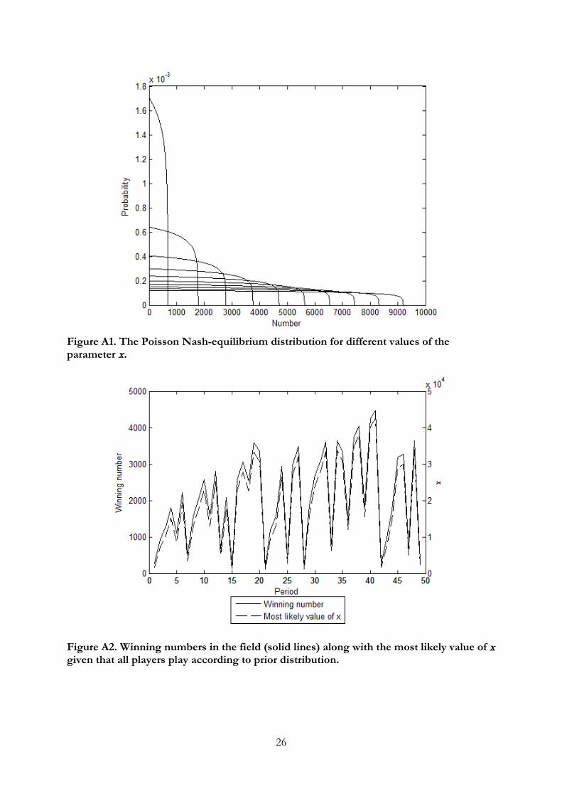
26

Figure A1. The Poisson Nash-equilibrium distribution for different values of the parameter x.

Figure A2. Winning numbers in the field (solid lines) along with the most likely value of x given that all players play according to prior distribution.

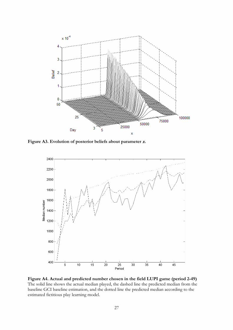
27

Figure A3. Evolution of posterior beliefs about parameter x.

Figure A4. Actual and predicted number chosen in the field LUPI game (period 2-49) The solid line shows the actual median played, the dashed line the predicted median from the baseline GCI baseline estimation, and the dotted line the predicted median according to the estimated fictitious play learning model.

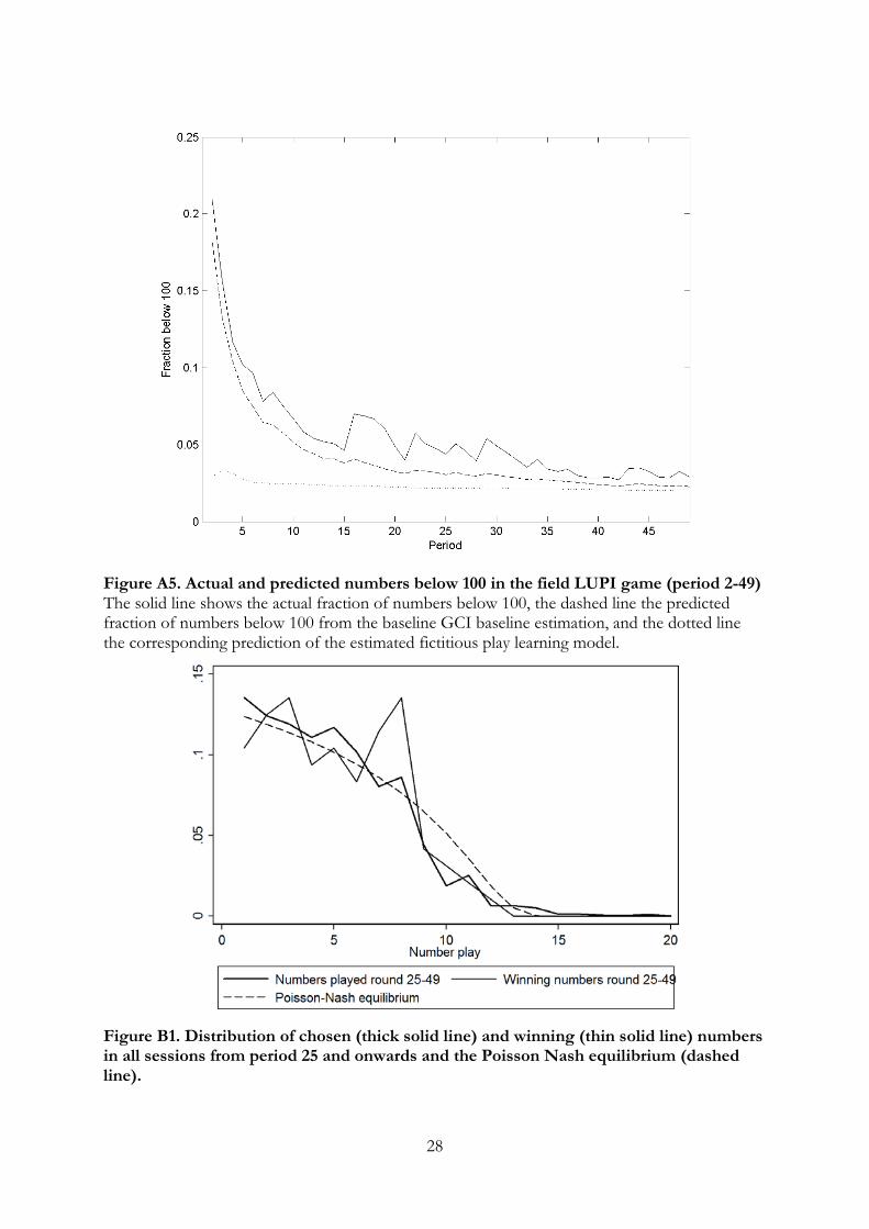
28

Figure A5. Actual and predicted numbers below 100 in the field LUPI game (period 2-49) The solid line shows the actual fraction of numbers below 100, the dashed line the predicted fraction of numbers below 100 from the baseline GCI baseline estimation, and the dotted line the corresponding prediction of the estimated fictitious play learning model.

Figure B1. Distribution of chosen (thick solid line) and winning (thin solid line) numbers in all sessions from period 25 and onwards and the Poisson Nash equilibrium (dashed line).

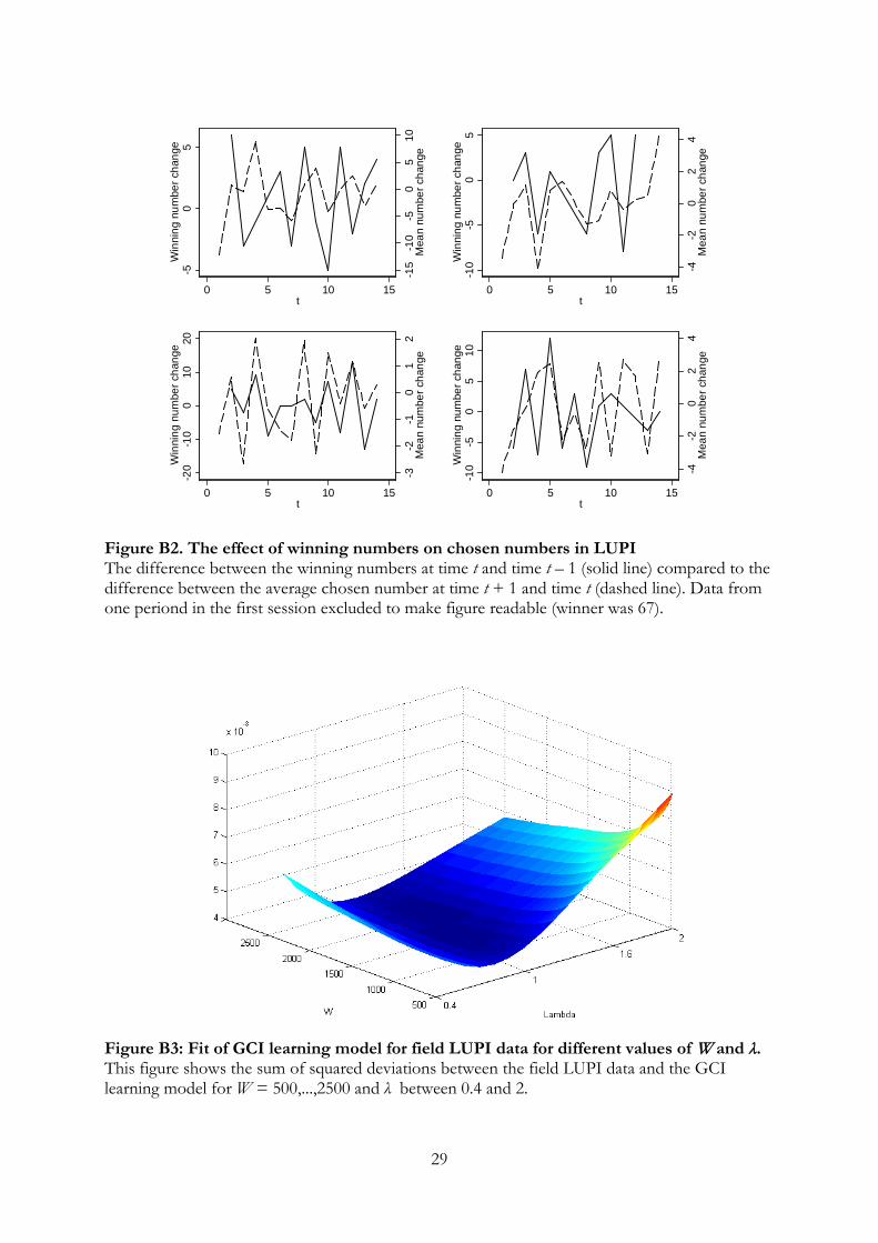
29

-15

-10

-50

510

Mea

n nu

mbe

r cha

nge

-50

5W

inni

ng n

umbe

r cha

nge

0 5 10 15t

-4-2

02

4M

ean

num

ber c

hang

e

-10

-50

5W

inni

ng n

umbe

r cha

nge

0 5 10 15t

-3-2

-10

12

Mea

n nu

mbe

r cha

nge

-20

-10

010

20W

inni

ng n

umbe

r cha

nge

0 5 10 15t

-4-2

02

4M

ean

num

ber c

hang

e

-10

-50

510

Win

ning

num

ber c

hang

e

0 5 10 15t

Figure B2. The effect of winning numbers on chosen numbers in LUPI The difference between the winning numbers at time t and time t – 1 (solid line) compared to the difference between the average chosen number at time t + 1 and time t (dashed line). Data from one periond in the first session excluded to make figure readable (winner was 67).

Figure B3: Fit of GCI learning model for field LUPI data for different values of W and λ. This figure shows the sum of squared deviations between the field LUPI data and the GCI learning model for W = 500,...,2500 and λ between 0.4 and 2.

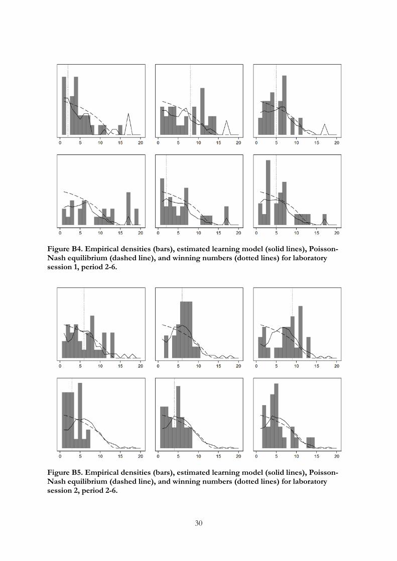
30

Figure B4. Empirical densities (bars), estimated learning model (solid lines), Poisson-Nash equilibrium (dashed line), and winning numbers (dotted lines) for laboratory session 1, period 2-6.

Figure B5. Empirical densities (bars), estimated learning model (solid lines), Poisson-Nash equilibrium (dashed line), and winning numbers (dotted lines) for laboratory session 2, period 2-6.

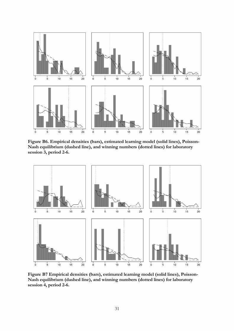
31

Figure B6. Empirical densities (bars), estimated learning model (solid lines), Poisson-Nash equilibrium (dashed line), and winning numbers (dotted lines) for laboratory session 3, period 2-6.

Figure B7 Empirical densities (bars), estimated learning model (solid lines), Poisson-Nash equilibrium (dashed line), and winning numbers (dotted lines) for laboratory session 4, period 2-6.

32

Figure B8: Fit of GCI learning model for laboratory LUPI data for different values of W and λ. This figure corresponds to Table 6 and shows the sum of squared deviations between period 1-7 in LUPI data and the GCI learning model for W = 5,...,15 and λ between 0.5 and 2.

Figure B9: The effect of winning numbers on chosen numbers in SLUPI, pmBC and CUPI. The difference between the winning numbers at time t and time t – 1 (solid line) compared to the difference between the average chosen number at time t + 1 and time t (dashed line). Winning numbers that change more than 10 numbers is shown as 10/-10 in graph. The strategy space in CUPI has been transformed as described in the main text.

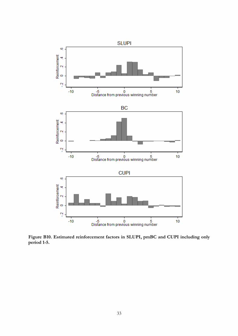
33

Figure B10. Estimated reinforcement factors in SLUPI, pmBC and CUPI including only period 1-5.

34

Figure C1. Figure included in the CUPI game instructions.

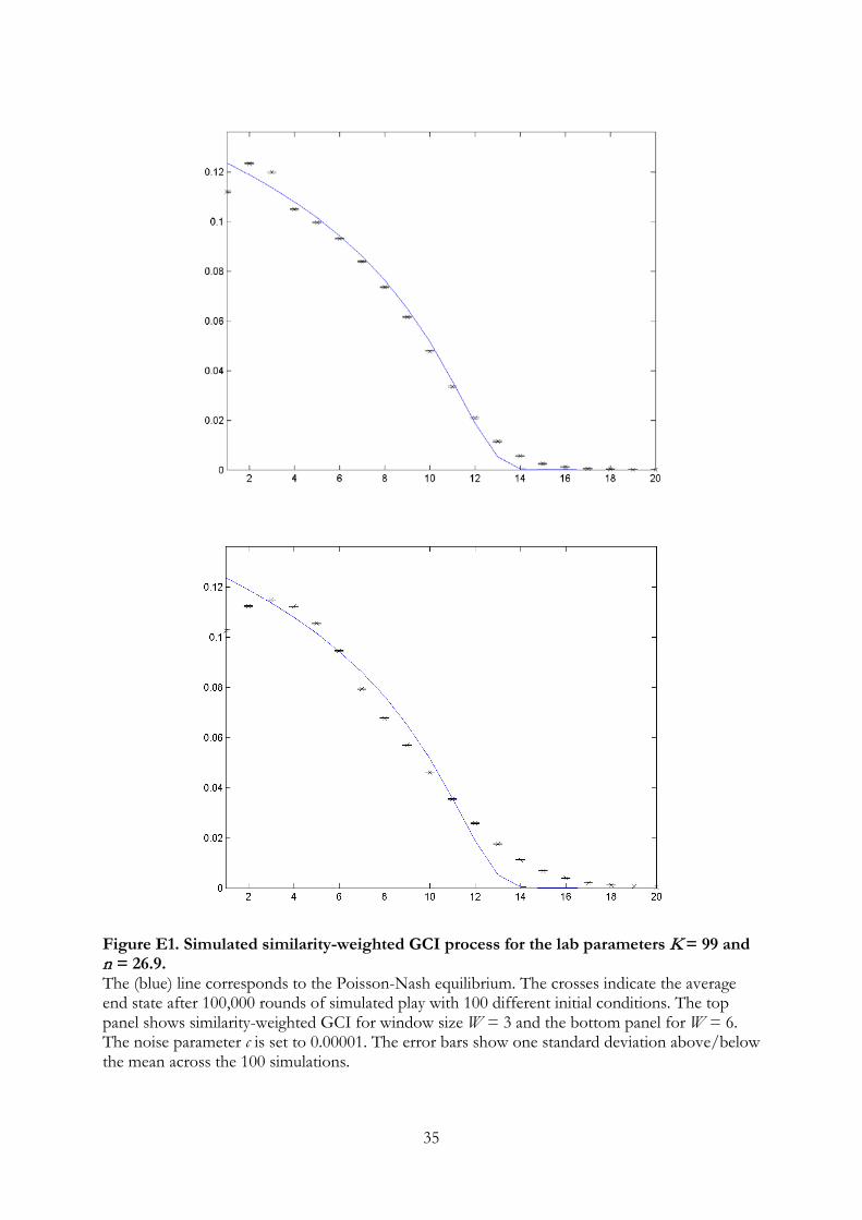
35

Figure E1. Simulated similarity-weighted GCI process for the lab parameters K = 99 and n = 26.9. The (blue) line corresponds to the Poisson-Nash equilibrium. The crosses indicate the average end state after 100,000 rounds of simulated play with 100 different initial conditions. The top panel shows similarity-weighted GCI for window size W = 3 and the bottom panel for W = 6. The noise parameter c is set to 0.00001. The error bars show one standard deviation above/below the mean across the 100 simulations.

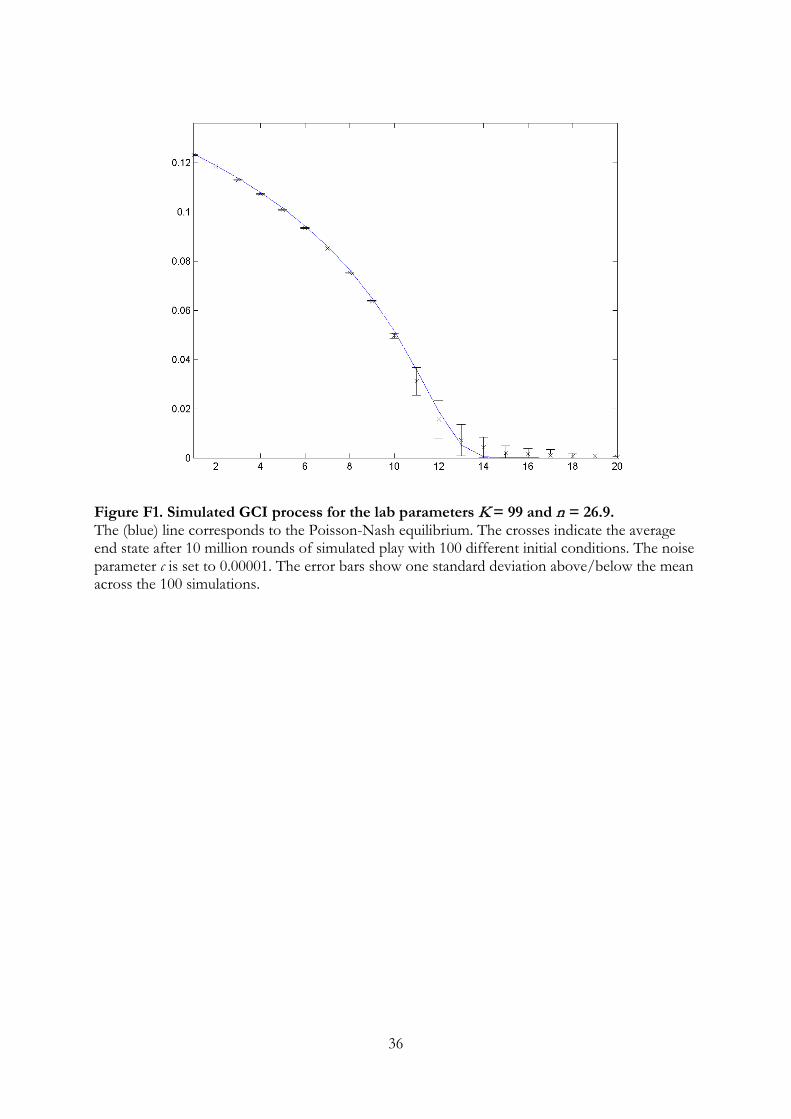
36

Figure F1. Simulated GCI process for the lab parameters K = 99 and n = 26.9. The (blue) line corresponds to the Poisson-Nash equilibrium. The crosses indicate the average end state after 10 million rounds of simulated play with 100 different initial conditions. The noise parameter c is set to 0.00001. The error bars show one standard deviation above/below the mean across the 100 simulations.