LEARNING THEORY

One of the important issues in repetitive operations is the effect of learning. It is obvious

that a repetitive operation offers better opportunities to achieve higher productivity. It is

widely recognized that labor productivity improves when repetition is involved in an

operation. It is widely accepted that production rates and/or productivity for performing

repetitive construction tasks will improve with additional experience and practice. That

is, the time and effort expended to complete repetitive activities decrease as the number

of repetitions increases. This phenomenon is usually referred to as learning curve effect,

or learning curve theory. So, learning is defined as: the improvement that results when

people repeat a process and gain skill or efficiency from the experience. There are several

reasons for this phenomenon:

Increased worker familiarization.

Improved equipment and crew coordination.

Improved job organization.

Better engineering support.

Better day-to-day management and supervision

Development of more efficient techniques and methods.

Development of more efficient material supply and handling systems.

Stabilized design leading to fewer modifications and rework.

Learning theory states that whenever the quantity of a product doubles, the unit or

cumulative average cost-hour, man-hour, dollars, etc. will decline by a certain

percentage. This percentage is called the learning rate which identifies the learning

achieved. It establishes also the slope of the learning curve. As shown in Fig. 1, a

learning rate of 100% means that no learning takes place. The lower the learning rate, the

greater the learning gain.

In large-scale repetitive projects, improvement occurs smoothly and continuously. The

phenomenon is real and has a specific application in cost analysis, cost estimating, or

profitability studies related to examination of future costs and confidence level in

analysis. The learning curve theory is a powerful tool for predicting, guiding, and

encouraging increases in productivity. Learning curves are set of equations that describe

the patterns of ongoing improvement found in many stable processes. As a set of

equations, learning curves describe specific patterns of improvement that can be used to

predict future productivity.

Fig. 1: Learning Curves of Straight-Line Model with Different Learning Rate

Learning Models Assumption

The learning theory is based on the following assumption:

• The time or the cost required for a given target or one unit of product to be

completed will be less each time when the target is achieved or the accumulated

production is increased.

• The time or the cost will be decreased in a declining distribution.

• The reduction of time or cost will follow a foreseeable distribution.

It is suggested that three factors need to be present for learning to take place:

• There should be something sufficiently complex about the operation to facilitate

learning.

• There should be repetition in the units being constructed.

• Management must create a stable work environment.

Factors Affecting Learning Rates

The most effective factors that influence the learning rate are schematically shown in Fig.

2 and discussed briefly in the following sections.

Fig. 2: Factors Affecting Learning Rates

Characteristics of the Task

The nature of the task usually has the greatest impact. Sub-factors like Task Complexity,

Newness, Dangerousness, Hazards, and Boredom dictate the characteristics of the task.

For example; the level of hazard associated with a given task can be measured with the

level of dust, radiation, or pressure encountered.

The Skill of Management on Job Site

Planning strategies, incentive motivation programs, safety precautions, responsibility

changes, level of supervision and inspection and availability of required materials and

tools are management-related sub-factors. An effective planning system and a good

management team can induce a climate in which learning will be relatively fast.

Adequate management supervision, motivation, and an incentive program will further aid

in achieving the accomplishment of this objective. On the other hand, inadequate

planning can cause inefficiency and errors in the completed tasks. This, if not corrected,

will cause an unsatisfactory rate of learning.

Characteristics of Labor on Site

Morale level, skills and coherence among crew member are sub-factors that determine

the characteristics of labor. A high morale level reflects a positive environment that

encourages learning development. Labor that possesses good skills and intelligence will

result in a quick learning development. The absence of these sub factors yields a negative

influence on learning improvement.

Project Characteristics

Circumstances around the project such as weather conditions, altitude of work,

accessibility of work site, equipment breakdowns, Interruption (e.g., accidents and

holidays), Project size, Noise and Project location define the characteristics of the project

that have a major effect on learning rate. For example, with an increase in the

altitude/height of the working area - as in high-rise buildings- fear of heights will have an

influence on both productivity of labor and enhancement of learning skills. Like

management, the influence of these external sub-factors will affect the learning

development of all crews involved.

In order to specify a learning rate for each task, analysis of these various factors and sub

factors collectively must be taken into account. Among all previous factors,

characteristics of the task itself often have the greatest impact.

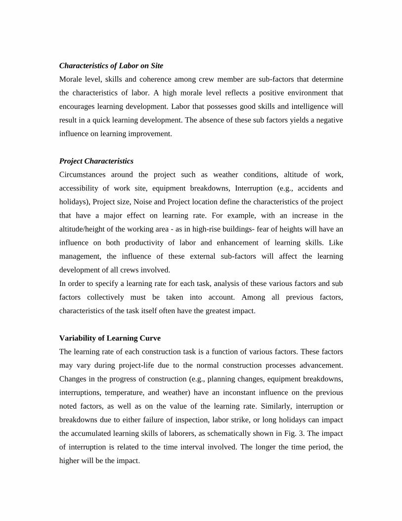
Variability of Learning Curve

The learning rate of each construction task is a function of various factors. These factors

may vary during project-life due to the normal construction processes advancement.

Changes in the progress of construction (e.g., planning changes, equipment breakdowns,

interruptions, temperature, and weather) have an inconstant influence on the previous

noted factors, as well as on the value of the learning rate. Similarly, interruption or

breakdowns due to either failure of inspection, labor strike, or long holidays can impact

the accumulated learning skills of laborers, as schematically shown in Fig. 3. The impact

of interruption is related to the time interval involved. The longer the time period, the

higher will be the impact.

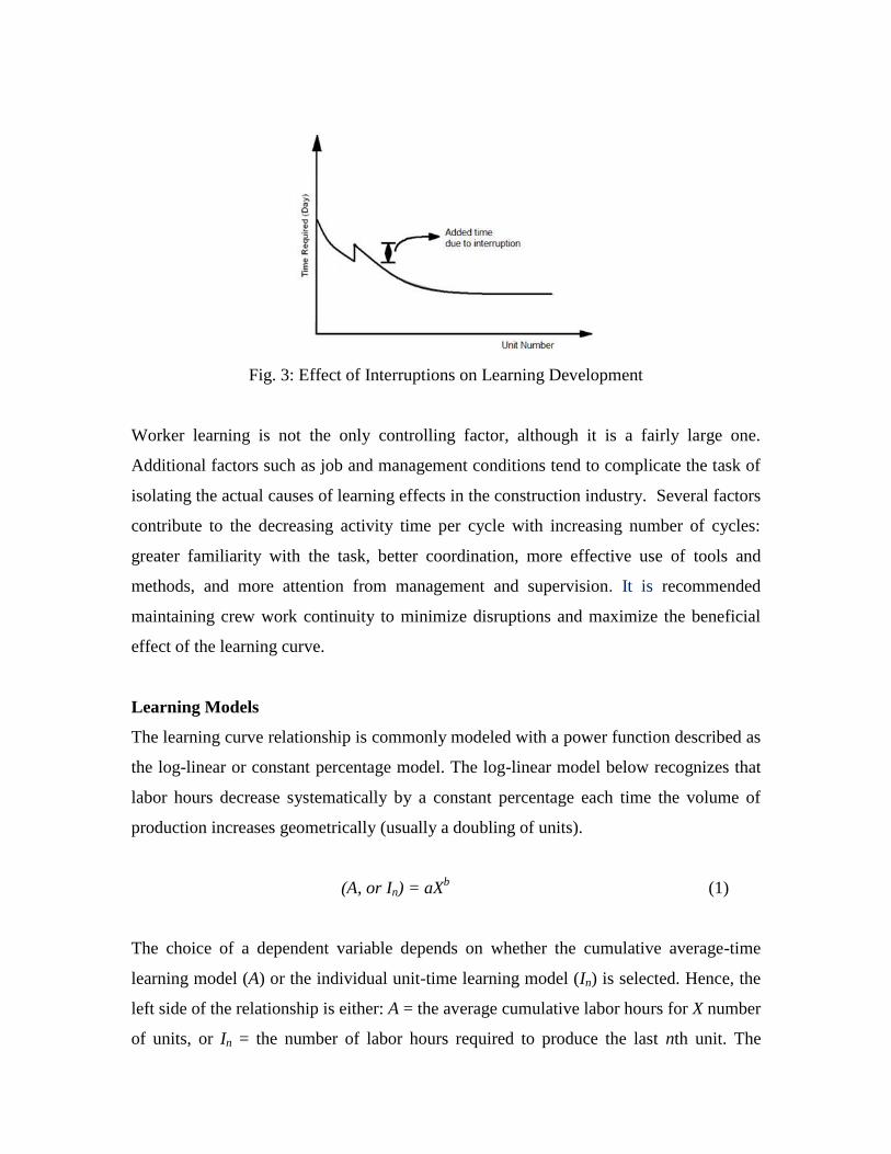
Fig. 3: Effect of Interruptions on Learning Development

Worker learning is not the only controlling factor, although it is a fairly large one.

Additional factors such as job and management conditions tend to complicate the task of

isolating the actual causes of learning effects in the construction industry. Several factors

contribute to the decreasing activity time per cycle with increasing number of cycles:

greater familiarity with the task, better coordination, more effective use of tools and

methods, and more attention from management and supervision. It is recommended

maintaining crew work continuity to minimize disruptions and maximize the beneficial

effect of the learning curve.

Learning Models

The learning curve relationship is commonly modeled with a power function described as

the log-linear or constant percentage model. The log-linear model below recognizes that

labor hours decrease systematically by a constant percentage each time the volume of

production increases geometrically (usually a doubling of units).

(A, or In) = aXb (1)

The choice of a dependent variable depends on whether the cumulative average-time

learning model (A) or the individual unit-time learning model (In) is selected. Hence, the

left side of the relationship is either: A = the average cumulative labor hours for X number

of units, or In = the number of labor hours required to produce the last nth unit. The

independent variables are defined as: a = the number of labor hours required to produce

the first unit, X = cumulative number of units produced, and b = learning exponent, which

is always negative. The negative learning exponent b is (log r)/(log f), where r is the rate

of learning represented by the constant percentage decrease in hours, and f is the factor

increase in output (usually in terms of 2). For example, an 80% learning rate with a

doubling of units has a learning exponent b equal to –0.3219, which is (log .80)/(log 2).

There are five basic mathematical models for learning curves. The various models are:

(1) The straight-line model; (2) the Stanford "B" model; (3) the cubic power model; (4)

the piecewise (or stepwise) model; and (5) the exponential model. These models are

shown graphically in Fig. 4.

Fig. 4: Common Learning Models

Figure 5 shows a hypothetical learning curve that is divided into two phases. The first is

the initial operation-learning phase, during which labor productivity increases rapidly as

workers acquire sufficient knowledge of the task to be performed. The second is routine-

acquiring phase, during which a more gradual improvement in labor productivity is

attained through a growing familiarity with the job and through refinements in methods,

organization, etc. Some models account for the effect of prior experience and a leveling-

off or stabilization of the process. The point Xp1 denotes the end of the acquired-

experience phase while point Xp2 is called the standard production point which marks the

end of the learning effect. Beyond this point, no further productivity improvements are

realized.

Fig. 5: Logarithmic Plot of a Hypothetical Learning Curve

Of the five models, the straight model are based upon the assumption that the learning

rate is a constant value (except for previous-experience adjustments in the Stanford "B"

model). However, several researchers have shown that the learning rate is not constant

throughout the progress of an activity. When the acquired experience factor and the

productivity leveling-off effect are both present, the result is an S-shaped curve.

The S-shaped curves like the cubic and piecewise models statistically describe production

and productivity data better than straight-line curves. The manufacture of missiles, space

vehicles, jet engines and electronic components, which generally have high learning rates

very early in the manufacturing program. High learning rates are usually due to acquired

experience with similar products. After the effect of the experience factor diminishes, the

learning rate decreases, which means that the cumulative man-hours per unit also

decrease at an accelerated rate. Once production has reached the so-called standard

production point, Xp2, the cumulative man-hours per unit stabilize. Thereafter, the

learning rate is 100%, and no further productivity improvement is realized.

Straight-Line Model

The straight-line learning curve model is the most commonly used model for construction

activities. The straight-line model is so named because it forms a straight line when

plotted on a Log-Log scale. The underlying assumption of the straight-line model is that

the learning rate remains constant throughout the duration of the activity. The original

straight-line learning curve was developed in 1936 by T. P. Wright. It was expressed as a

straight-line cumulative average model given by Eq. 2

Yca = AX-n

…..……………………… …………………… …. (2)

where Yca is cumulative average cost, man-hour or time per unit.

A is cost, man-hour or time required for the first unit.

X is unit or sequence number.

n is slope of logarithmic curve.

Stanford "B" Model

The Stanford "B" model assumes that the straight-line model is the normal situation

provided the crew have no acquired experience. Acquired experience is defined as the

"know how" or experience, resulting from performing similar activities or constructing

similar units in the immediate past. The Stanford "B" model is therefore a modification of

the straight-line model to account for acquired experience. This experience causes

productivity gains to be less during the operation-learning phase, as shown in Fig. 5.

Thereafter, the learning rate will decrease to reflect an overall improvement in

productivity. The Stanford "B" model is mathematically expressed by Eq. 3.

Yca = A(X + B)-n

…………………………… …….………………..... (3)

where Yca, A, X and n are the same as in Eq. 2, while B is a factor describing the

crew's acquired experience. A crew with no prior experience will have a B factor

of zero, while an experienced crew may have an experience factor of four or

higher. The B factor is defined as the equivalent number of units' worth of

experience.

Cubic Model

The cubic model assumes that the learning rate is not a constant variable because of the

combined effects of previous experience and the leveling-off of productivity as the

activity nears completion. The equation for the cubic learning curve model is given by

Eq. 4.

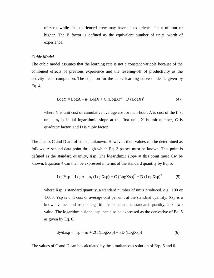
LogY = LogA – n1 LogX + C (LogX)2 + D (LogX)

3 ………………… (4)

where Y is unit cost or cumulative average cost or man-hour, A is cost of the first

unit , n1 is initial logarithmic slope at the first unit, X is unit number, C is

quadratic factor, and D is cubic factor.

The factors C and D are of course unknown. However, their values can be determined as

follows. A second data point through which Eq. 3 passes must be known. This point is

defined as the standard quantity, Xsp. The logarithmic slope at this point must also be

known. Equation 4 can then be expressed in terms of the standard quantity by Eq. 5.

LogYsp = LogA – n1 (LogXsp) + C (LogXsp)2 + D (LogXsp)

3……… (5)

where Xsp is standard quantity, a standard number of units produced, e.g., 100 or

1,000; Ysp is unit cost or average cost per unit at the standard quantity, Xsp is a

known value; and nsp is logarithmic slope at the standard quantity, a known

value. The logarithmic slope, nsp, can also be expressed as the derivative of Eq. 5

as given by Eq. 6.

dy/dxsp = nsp = n1 + 2C (LogXsp) + 3D (LogXsp)…...… .… .… .… (6)

The values of C and D can be calculated by the simultaneous solution of Eqs. 5 and 6.

Cubic learning curve models have been shown to provide the best statistical fit for

empirical data from the electronics industry.

Piecewise (or Stepwise) Model

The piecewise model is a linearized approximation of the cubic model. The equation for

the piecewise curve is given by Eq. 7.

LogY=LogA–n1 LogX- n2 J1(LogX-LogXp1)- n3J2(LogX-LogXp2)……….. (7)

where Y is unit or cumulative average cost, man-hour or time; X is unit number;

n1 is slope of the first segment; J1 is 1 if X > Xp1 , 0 otherwise; n2 is additional

slope of the second segment, total slope = n1+n2; J2= 1 if X>Xp2, 0 otherwise; n3

is additional slope of the third segment, total slope is n1+n2+n3; Xp1 is first point

where the slope changes, usually in the operation-learning phase (Fig. 5); and Xp2

is second point where the slope changes, the end of the routine-acquiring phase.

This is called the standard production point.

Exponential Model

A United Nations report described an exponential learning curve function developed by

the Norwegian Building Research Institute. It is based upon the rule that the part of the

cost per unit that can be reduced by repetition will be reduced by one-half after a constant

number of repetitions. The unit cost is defined by Eq. 8:

Yu= Yult + (A-Yult)/2(X/H) ……………………………….………... (8)

where Yu is unit cost, man-hour or time for unit X; Yult is ultimate or lowest cost,

man-hour or time per unit at the end of the routine-acquiring phase; A is cost,

man-hour or time of first unit; X is unit number and H is a constant "Halving

Factor," which is the number of units required for that part of the unit cost that

can be reduced by repetition to one-half. A learning curve model for cumulative

data was not presented.

Data Representation in Learning Curve Theory

The analyst has to choose from several methods of representing data, usually trading-off

between response and stability of forecasting information. Traditionally, learning curve

data has been represented using either unit data or cumulative-average data. There are

two other techniques: the moving average and the exponentially weighted average.

Unit Data

Unit data is the time or cost to complete a given cycle versus the cycle number. It shows

the actual performance of the repetitive activity exactly as it happened, when it happened.

This is the raw data in its simplest form. Fig. 6 shows highly variable unit data for setting

466 precast concrete floor planks in apartment building projects. It is apparent that no

clear relation exists. Unfortunately, for many construction activities, there may be a great

deal of noise or scatter in the data. When the learning curve is plotted, trends may not be

readily apparent to the construction manager trying to forecast future performance.

Fig. 6: Unit Plot for Setting Floor Planks

The Cumulative Average Data

The cumulative average data is the average time or cost to complete all cycles up to and

including the given cycle versus the cycle number. It helps smooth out some of the noisy

in the data by averaging many cycles together. Long-term trends become much more

obvious. Short-term trends, however, may be hidden. As more and more cycles are

incorporated into the data set, the most recent cycle or cycles are discounted and

contribute relatively little to the overall cumulative average. Figure 7 shows the same

process for cumulative average data of setting 466 precast concrete floor planks in

apartment building projects. The predictive capabilities are obviously enhanced using the

cumulative average data.

Fig. 7: Cumulative Average Plot for Setting Precast Concrete Floor Planks

Mathematically cumulative average (CA) can be calculated by Eq. 9.

CAi = (X1 + X2 + x3 + ….. + Xi)/i (9)

where i is the cycle no.

CAi is the cumulative average at cycle no. i

X1 , X2 , x3 , ….. , Xi are the corresponding (unit data)

When all of the data points arrive (i = K(total number of cycles)), the cumulative average

will equal the final average.

Moving Average

Moving average is a variation on the cumulative average, the difference being that only

the most recent data are included in the average. The analyst must decide how far back in

time the data are still significant when choosing how many cycles to incorporate in the

moving average. This decision may be based on the amount of scatter (more points will

help smooth the curve), and the importance of very short-term trends (too many points

will hide the short-term trends, too few points may have too much scatter). The extreme

cases of the moving average are unit data (a moving average of one point), and the

cumulative-average data (a moving average of a very large number of points). The

moving average is, then, a compromise of sorts between the unit data and the cumulative-

average data.

Mathematically moving average (MA) can be calculated by Eq. 10.

where N is the number of cycles which used in the calculation

MAt is the moving average production rate of order N at cycle t

Yt-N+1+ … + Yt-1 + Yt are the corresponding production rate (unit data)

t is cycle number

The Exponentially Weighted Average

The exponentially weighted average is based on the concept of computing a weighted

average of: (1) the most recent data; and (2) the previous average. The previous average

contains information about all prior cycles and should be counted more heavily than a

single new observation. Mathematically Exponentially Weighted Average (EWA) can be

calculated by Eq. 11.

Where EWAt is exponentially weighted average at cycle t

0 < α < 1 is the smoothing constant for example 0.1, 0.3 or 0.4.

10

11

Selection of the value for α is analogous to selecting the number of cycles to include in an

un-weighted moving average. Larger values of α will make the new average change more

quickly if new data are substantially different than the old. For the same reason, larger

values of α will cause the new average to respond, and possibly over respond, to new

data. Thus, the choice of α is a trade-off between response and stability. Although the

moving average and the exponentially weighted average are widely used in a variety of

disciplines - such as technical analysis of financial data, like stock prices and in

economics to examine gross domestic product- they have not been applied to learning-

curve research.

Example

To illustrate how each of the four data represented methods is implemented, a numerical

example is used. The unit data are given for 17 successive cycles in column 2 of the

following table. In column 3, cumulative are computed for the unit data from which

cumulative average is computed in column 4. For example, cumulative average at cycle 4

is calculated as: 8.444/4=2.111.

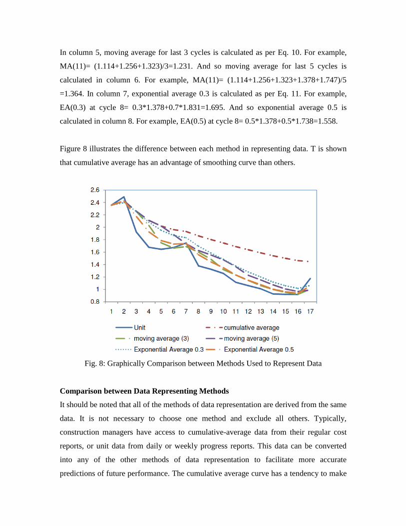
In column 5, moving average for last 3 cycles is calculated as per Eq. 10. For example,

MA(11)= (1.114+1.256+1.323)/3=1.231. And so moving average for last 5 cycles is

calculated in column 6. For example, MA(11)= (1.114+1.256+1.323+1.378+1.747)/5

=1.364. In column 7, exponential average 0.3 is calculated as per Eq. 11. For example,

EA(0.3) at cycle 8= 0.3*1.378+0.7*1.831=1.695. And so exponential average 0.5 is

calculated in column 8. For example, EA(0.5) at cycle 8= 0.5*1.378+0.5*1.738=1.558.

Figure 8 illustrates the difference between each method in representing data. T is shown

that cumulative average has an advantage of smoothing curve than others.

Fig. 8: Graphically Comparison between Methods Used to Represent Data

Comparison between Data Representing Methods

It should be noted that all of the methods of data representation are derived from the same

data. It is not necessary to choose one method and exclude all others. Typically,

construction managers have access to cumulative-average data from their regular cost

reports, or unit data from daily or weekly progress reports. This data can be converted

into any of the other methods of data representation to facilitate more accurate

predictions of future performance. The cumulative average curve has a tendency to make

the basic data look better (smaller variation) than similar curves using unit data.

However, the cumulative average and unit curves are complementary rather than

competing forms, because both are derivatives of the same data.

Using Learning Curves to Predict Future Performance

The greatest potential value of learning curves is their ability to predict future

performance, instead of fitting historical data. The linear model provides the best

correlation between actual and predicted performance for the models and activities tested.

The cubic models that best correlate to historical data are shown to be poor predictors of

future performance according to testing sensitivity of extensions of cubic and linear curve

model to number of points for best fit curve founding that cubic curve model is sensitive

to the number of cycles used to derive the equation vice versa linear curve model.

The accuracy of predicting the time or cost required to complete an ongoing activity

improves dramatically for about the first 25-30% of the activity and then levels off to

within 15-20% of the actual value. Predicting performance of contractors is of interest to

both academics and practitioners. The physical execution of a project is critical to the

overall success of the development.

Forgetting Phenomenon

The routine-acquiring process is delayed for even a short time, some of the experience

curve effect is lost, although upon resumption of the activity, the routine-acquiring

process resumes at the same decremented rate. This is known by forgetting phenomenon.

It assumed that an individual's memory is the equivalent of storing electrical charges in

the brain. Following a similar logic, the forgetting portion of the learning cycle can be

described by a negative decay function comparable to the decay observed in electrical

losses in condensers. Some forgetting is always expected but total forgetting do not

occurs within short periods of interruption. Forgetting curve shows rapid initial decrease

in performance followed by a gradual leveling-off. The rate and amount of forgetting

decrease as an increase of number of units completed before an interruption occurs.

When the interruption is sufficiently long, there is nothing more to forget, since

everything has already been forgotten. The forgetting phenomenon is illustrated in Fig. 9.

Fig. 9: S-Shaped Forgetting Curve

The typical learning-forgetting-learning model is composed of two learning curves and

one forgetting curve, as shown in Fig. 10

Fig. 10: Graphical Presentation of the Learning-Forgetting-Learning Curve

As indicated, the curves with a positive slope are learning curves, whereas the one with a

negative slope is the forgetting curve. The slope of the curved bands for the learning-

forgetting case after the interruption is lower than the learning case.

The application of the learning and forgetting effects may enable planning and

arrangement of the sequence of different tasks to be more accurate and reliable. Such

improved techniques can enhance the smooth running of construction among a large

number of conflicting activities and minimize the chance of activities crashing. With this

improved master program, different sub-contractors can plan their human and material

resources more accurately and can fulfill their respective duties in a timely manner. This

may, in turn, make the overall construction period more reliable

Most contractors have experienced delays in schedule as a result of slow initial

construction operations, before learning has been taken place. However, most can

overcome delays during the course of construction. Moreover, although learning and

forgetting take place after an interruption occurs, the measurement of productivity

remains unchanged after the interruption.

Example

Raw data

Fig. 11: Daily Production

Modified Data

It is noticed that weekly production values increases generally. However for week 4 the

weekly production decreases rapidly. It may be due to management problems or lack of

materials. Also, the production decreases at weeks 23, 24 and 25 because of forgetting

phenomenon.

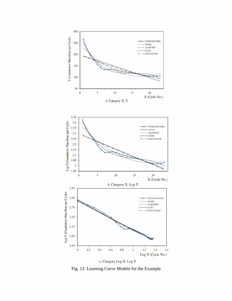
Fig. 12: Learning Curve Models for the Example

Figure 12 shows the graphical representation of the 12 Learning Curve Models given in

the previous table. It can be observed from Figure 12, that man-hour per cycle decreases

rapidly in the first seven cycles referring to learning effect in addition to past experience

and prior preparation. Starting from cycle 8 to cycle 9, man-hour per cycle is almost

steady which is defined as leveling-off or stabilization of the process. In addition, man-

hour per cycle decreases generally till about cycle 21. However the last two cycles, it can

be observed the routine acquiring phenomenon which represent as increasing in man-

hour per cycle.

References

Adler, P. S. and Clark K. B. (1991). “Behind the Learning Curve: A Sketch of the

Learning Process.” Management Science, Vol. 37, No. 3, pp. 267–281.

Carlson, J. (1973). “Cubic Learning Curves: Precision Tool for Labor Estimating.”

Manufacturing Engineering and Management, Vol. 67, No. 11, pp. 22–25.

Carlson, J. G. and Rowe, A. J. (1976). “How Much Does Forgetting Cost.” Industrial

Engineering, Vol. 8, No. 9, pp. 40-47.

Cochran, E. B. (1960). “New Concepts of the Learning Curve.” Journal of Industrial

Engineering, Vol. 4, pp. 317-327.

Couto, J. P. and Teixeira, J. C. (2005). “Using Linear Model for Learning Curve Effect

on High Rise Floor Construction.” Journal of Construction Management and

Economics, Vol. 23, pp. 355-364.

Everett, J. G. and Farghal S. (1997). “Data Representation for Predicting Performance

with Learning Curves.” Journal of Construction Engineering and Management,

ASCE, Vol. 123, No. 1, pp. 46-52.

Humphreys, K. K. (1998). Jellen’s Cost and Optimization Engineering. McGraw-Hill,

Inc., New York, USA.

Ismail, M.S, (2011). Investigation of Learning Curve Effect on Pipeline Construction in

Egypt. Master Thesis, Structural Engineering Department, Tanta University, Tanta,

Egypt.

Lam, K. C., Lee, D. and Hu, T. (2001). “Understanding the Effect of the Learning-

Forgetting Phenomenon to Duration of Projects Construction.” International Journal

of Project Management, Vol. 19, pp. 411-420.

Oglesby, C. H., Parker, H. W. and Howell, G. A. (1989). Productivity Improvement in

Construction. McGraw-Hill, New York, USA.

Thomas, H. R. (2009). “Construction Learning Curves.” Practice Periodical on

Structural Design and Construction, Vol. 14, No. 1, pp. 14-20.

Thomas, H. R., Mathews, C. T., and Ward, J. G. (1986). “Learning Curve Models of

Construction Productivity.” Journal of Construction Engineering and Management,

ASCE, Vol. 112, No. 2, pp. 245-258.

Wong, P. S. P., Cheung, S. O. and Hardcastle, C. (2007). “Embodying Learning Effect in

Performance Prediction.” Journal of Construction Engineering and Management,

ASCE, Vol. 133, No. 6, pp. 474–482.