Learning Specific-Class Segmentation from Diverse Data

M. Pawan Kumar Haithem Turki Dan Preston Daphne Koller

Computer Science Department

Stanford University

{pawan,hturki,dpreston,koller}@cs.stanford.edu

Abstract

We consider the task of learning the parameters of a seg-

mentation model that assigns a specific semantic class to

each pixel of a given image. The main problem we face is

the lack of fully supervised data. We address this issue by

developing a principled framework for learning the param-

eters of a specific-class segmentation model using diverse

data. More precisely, we propose a latent structural sup-

port vector machine formulation, where the latent variables

model any missing information in the human annotation. Of

particular interest to us are three types of annotations: (i)

images segmented using generic foreground or background

classes; (ii) images with bounding boxes specified for ob-

jects; and (iii) images labeled to indicate the presence of

a class. Using large, publicly available datasets we show

that our approach is able to exploit the information present

in different annotations to improve the accuracy of a state-

of-the art region-based model.

1. Introduction and Related Work

Specific-class segmentation offers a useful representa-

tion of the scene by assigning each pixel of a given image

to a specific semantic class (for example, ‘person’, ‘build-

ing’ or ‘tree’). While computer vision has made great

strides in developing sophisticated models for this prob-

lem [8, 9, 10, 12, 16, 17, 19, 21, 22, 23], learning the param-

eters of such models still remains a challenge. The training

regimes currently used can be broadly divided into two cat-

egories: (i) training with only segmented images, for exam-

ple, the entries to the VOC challenge [6]; and (ii) training

with only weakly supervised data such as image-level la-

bels [1, 2, 3, 22]. The first category requires the collection

of fully supervised data—an onerous task, as indicated by

the use of generic class labels in current datasets. The sec-

ond category results in a difficult learning problem that has

so far only be solved in limited settings (small number of

classes, negligible background clutter).

The common drawback of existing methods is that they

do not truly reflect the availability of data in real life. On-

line tools, such as Amazon’s Mechanical Turk, allow us to

obtain cleanly segmented images at a low cost. The ease of

specifying bounding boxes or image-level labels has made

thousands of weakly supervised images available, which we

cannot afford to ignore. To overcome this drawback, we

make important contributions in the following three areas.

Problem Formulation. We design a principled framework

for learning with diverse data, with the aim of exploiting

the varying degrees of information in the different datasets

to the fullest: from the cleanliness of pixelwise segmenta-

tions, to the vast availability of bounding boxes and image-

level labels. Specifically, we formulate the parameter learn-

ing problem using a latent structural support vector machine

(LSVM) [7, 24], where the latent variables model any miss-

ing information in the annotation. For this work, we fo-

cus on three types of missing information: (i) the specific

class of a pixel labeled using a generic foreground or back-

ground class; (ii) the segmentation of an image annotated

with bounding boxes of objects; and (iii) the segmentation

of an image labeled to indicate the presence of a class.

Inference. We design accurate inference algorithms, which

are required to learn an LSVM, for a state-of-the-art region-

based model [9]. Our algorithms are able to complete the

annotation of weakly supervised images, thereby allowing

us to learn from them.

Learning. We empirically demonstrate that, unlike the

concave-convex procedure [7, 24] previously employed in

computer vision, our recently proposed self-paced learning

algorithm [14] is able to avoid bad local minimum solutions

when learning with diverse data.

We test our approach on a combination of four of the

largest datasets: (i) VOC2009 segmentation dataset [6], with

pixelwise segmentation for foreground classes; (ii) SBD [9],

with pixelwise segmentation for background classes; (iii)

VOC2010 detection dataset [6], with bounding boxes for in-

stances of foreground classes; and (iv) ImageNet [4], with

image-level labels for foreground classes.

2. Learning with Generic ClassesGiven a training dataset that consists of images with

different types of ground-truth annotations, our goal is to

learn accurate parameters for a specific-class segmentation

model. We begin by considering a general model to high-

light that our approach is applicable to several existing

model-based segmentation algorithms. In section 5 we will

provide the details for learning a region-based model [9].

1

To simplify the discussion, we first focus on the case

where the ground-truth annotation of an image specifies a

pixelwise segmentation that includes generic foreground or

background labels. As will be seen in sections 3 and 4, the

other cases of interest, where the ground-truth only speci-

fies bounding boxes for objects or image-level labels, will

be handled by solving a series of LSVM problems that deal

with generic class annotations.

Notation. Given an image x and a labeling (that is, a seg-

mentation specified by the model) y, we denote their joint

feature vector by Ψ(x,y). The energy of a segmentation

is equal to w⊤Ψ(x,y), where w are the parameters of the

model. The best segmentation of an image is obtained us-

ing MAP inference, that is, minimizing the energy to obtain

y∗ = argminy w⊤Ψ(x,y).We denote the training dataset as D = {(xk,ak), k =

1, · · · , n}, where xk is an image and ak is the correspond-

ing annotation. For each image x with annotation a, we

specify a set of latent, or hidden, variables h such that

{a,h} defines a labeling y of the model. In other words,

for each pixel p labeled using the generic foreground (back-

ground) class, the latent variable hp models its specific fore-

ground (background) class.

Learning as Risk Minimization. Given the dataset D, we

learn the parameters w by training an LSVM. Briefly, an

LSVM minimizes an upper bound on a user-specified risk, or

loss, ∆(a, {a, h}). Here, a is the ground-truth and {a, h}is the predicted segmentation for a given set of parameters.

In this work, we specify the loss using the overlap score,

which is the measure of accuracy for the VOC challenge [6].

For an image labeled using specific foreground classes and a

generic background (the label set denoted by F), we define

the loss function as

∆(a, {a, h}) = 1−1

|F|

∑

i∈F

∣

∣

∣Pi(a) ∩ Pi({a, h})

∣

∣

∣

∣

∣

∣Pi(a) ∪ Pi({a, h})

∣

∣

∣

, (1)

where the function Pi(·) returns the set of all the pixels la-

beled using class i. Note that when i is the generic back-

ground, then Pi({a, h}) is the set of all pixels labeled us-

ing any specific background class. A similar loss function

can be defined for images labeled using specific background

classes and a generic foreground (the label set B). Formally,

the parameters are learned by solving the following non-

convex optimization problem:

minw,ξk≥0

λ

2||w||2 +

1

n

n∑

k=1

ξk, (2)

s.t. maxh

w⊤(

Ψ(xk, {ak,hk})−Ψ(xk, {ak,h}))

≥ ∆(ak, {ak,hk})− ξk, ∀ak,hk.

Intuitively, the problem requires that for every image the

energy of the ground-truth annotation, augmented with the

best value of its latent variables, should be less than the en-

ergy of all other labelings. The desired margin between the

two energy values is proportional to the loss.

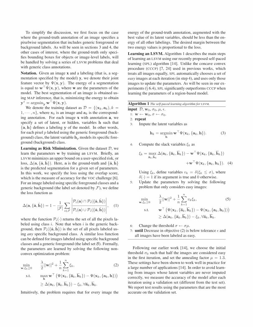
Learning an LSVM. Algorithm 1 describes the main steps

of learning an LSVM using our recently proposed self-paced

learning (SPL) algorithm [14]. Unlike the concave convex

procedure (CCCP) [7, 24] used in previous works, which

treats all images equally, SPL automatically chooses a set of

easy images at each iteration (in step 4), and uses only those

images to update the parameters. As will be seen in our ex-

periments (§ 6.4), SPL significantly outperforms CCCP when

learning the parameters of a region-based model.

Algorithm 1 The self-paced learning algorithm for LSVM.

input D, w0, σ0, µ, ǫ.

1: w← w0, σ ← σ0.

2: repeat

3: Impute the latent variables as

hk = argminh

w⊤Ψ(xk, {ak,h}). (3)

4: Compute the slack variables ξk as

ξk = maxak,hk

∆(ak, {ak,hk})−w⊤Ψ(xk, {ak,hk})

+w⊤Ψ(xk, {ak,hk}). (4)

Using ξk, define variables vk = δ(ξk ≤ σ), where

δ(·) = 1 if its argument is true and 0 otherwise.

5: Update the parameters by solving the following

problem that only considers easy images:

minw,ξk≥0

λ

2||w||2 +

1

n

n∑

k=1

vkξk, (5)

s.t. w⊤(

Ψ(xk, {ak,hk})−Ψ(xk, {ak,hk}))

≥ ∆(ak, {ak,hk})− ξk, ∀ak,hk.

6: Change the threshold σ ← σµ.

7: until Decrease in objective (2) is below tolerance ǫ and

all images have been labeled as easy.

Following our earlier work [14], we choose the initial

threshold σ0 such that half the images are considered easy

in the first iteration, and set the annealing factor µ = 1.3.

These settings have been shown to work well in practice for

a large number of applications [14]. In order to avoid learn-

ing from images whose latent variables are never imputed

correctly, we measure the accuracy of the model after each

iteration using a validation set (different from the test set).

We report test results using the parameters that are the most

accurate on the validation set.

Let us take a closer look at what is needed to learn the

parameters of our model. The first step of SPL requires us to

impute the latent variables of each training image x, given

the ground-truth annotation a, by solving problem (3). In

other words, this step completes the segmentation to pro-

vide us with a positive example. We call this annotation-

consistent inference. The second step requires us to find a

segmentation with low energy but high loss (a negative ex-

ample) by solving problem (4). We call this loss-augmented

inference. The third step requires solving the convex op-

timization problem (5). In this work, we solve it using

stochastic subgradient descent [20], where the subgradi-

ent for a given image is obtained by solving problem (4).

See [15] for details.

To summarize, in order to learn from generic class seg-

mentations, we require two types of inference algorithms—

annotation-consistent inference and loss-augmented infer-

ence. Both these types of inference algorithms can be

designed for several existing models by suitably modify-

ing their energy minimization algorithm. In section 5, we

describe these inference algorithms for the region-based

model used in our experiments (see Fig. 1(a) for example

segmentation obtained by annotation-consistent inference).

3. Learning with Bounding Boxes

We now focus on learning specific-class segmentation

from training images with user-specified bounding boxes

for instances of some classes. To simplify our description,

we make the following assumptions: (i) the image contains

only one bounding box, which provides us with the location

information for an instance of a specific foreground class;

and (ii) all the pixels that lie outside the bounding box be-

long to the generic background class. We note that our ap-

proach can be trivially extended to handle cases where the

above assumptions do not hold true (for example, bounding

boxes for background or multiple boxes per image).

The major obstacle in using bounding box annotations is

the lack of a readily available loss function that compares

bounding boxes b to pixelwise segmentations (a, h). Note

that it would be unwise to use a loss function that compares

two bounding boxes (the ground-truth and the predicted one

that can be derived from the segmentation), as this function

would not be compatible with the overlap score loss used in

the previous section. In other words, minimizing such a loss

function would not necessarily improve the segmentation

accuracy. We address this issue by adopting a simple, yet

effective, strategy that solves a series of LSVM problems for

generic classes. Our approach consists of three steps:

• Given an image x and its bounding box annotation b,

we infer its segmentation yB using the current set of

parameters (say, the parameters learned using generic

class segmentation data). The segmentation is ob-

tained by minimizing an objective function that aug-

ments the energy of the model with terms that encour-

age the segmentation to agree with the bounding box

(see details below).

• Using the above segmentation, we define a generic

class annotation a of the image (see details below).

• Annotations a are used to learn the parameters.

The new parameters then update the segmentation, and the

entire process is repeated until convergence (that is, until the

segmentations stop changing). Note that the third step sim-

ply involves learning an LSVM as described in the previous

section. We describe the first two steps in more detail.

Using the Bounding Box for Segmentation. We assume

that the specified bounding box is tight (a safe assumption

for most datasets) and penalize any row and column of the

bounding box that is not covered by the corresponding class.

Here, a row or column is said to be covered if it contains a

sufficient number of pixels s that have been assigned to the

corresponding class of the bounding box. Formally, given

a bounding box b of class c, we define an annotation a′

such that all the pixels p inside the bounding box have no

label specified in a′ (denoted by a′p = 0) and all the pixels

outside the bounding box have a generic background label

(consistent with our assumption). Furthermore, we define

latent variables h that model the specific semantic classes

for each pixel. Using a′ and b, we estimate h as follows:

h = argminh

w⊤Ψ(x, {a′,h}) +∑

q

κqIq(h, c). (6)

Here q indexes the rows and columns of b, and Iq is an

indicator function for whether q is covered by the latent

variables h. The penalty κq has a high value κmax for

the center row and center column, and decreases at a lin-

ear rate to κmin at the boundary. In our experiments, we

set κmax = 10κmin and cross-validated the value of κmin

using a small set of images. We found that our method pro-

duced very similar segmentations for a large range of κmin.

See [15] for examples.

We refer to problem (6) as bounding-box inference. Note

that Iq adds a higher-order potential to the energy of the

model since its value depends on the labels of all the pix-

els in a particular row or column. However, the potential

is sparse (that is, it only takes a non-zero value for a small

number of labelings). Hence, the above problem can be op-

timized efficiently [11]. We describe bounding-box infer-

ence for our region-based model in section 5 (see Fig. 1(b)

for example annotations).

From Segmentation to Annotation. Let yB = {a′,h}denote the labeling obtained from bounding-box inference.

Using yB we define an annotation a as follows. For each

pixel p inside the bounding box that was labeled as class c,

that is, yBp = c, we define ap = c. For pixels p inside the

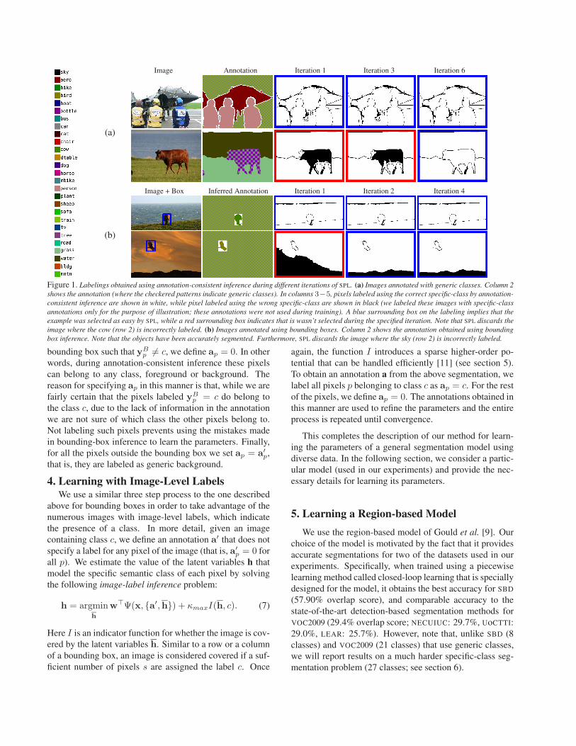
Image Annotation Iteration 1 Iteration 3 Iteration 6

(a)

Image + Box Inferred Annotation Iteration 1 Iteration 2 Iteration 4

(b)

Figure 1. Labelings obtained using annotation-consistent inference during different iterations of SPL. (a) Images annotated with generic classes. Column 2

shows the annotation (where the checkered patterns indicate generic classes). In columns 3−5, pixels labeled using the correct specific-class by annotation-

consistent inference are shown in white, while pixel labeled using the wrong specific-class are shown in black (we labeled these images with specific-class

annotations only for the purpose of illustration; these annotations were not used during training). A blue surrounding box on the labeling implies that the

example was selected as easy by SPL, while a red surrounding box indicates that is wasn’t selected during the specified iteration. Note that SPL discards the

image where the cow (row 2) is incorrectly labeled. (b) Images annotated using bounding boxes. Column 2 shows the annotation obtained using bounding

box inference. Note that the objects have been accurately segmented. Furthermore, SPL discards the image where the sky (row 2) is incorrectly labeled.

bounding box such that yBp 6= c, we define ap = 0. In other

words, during annotation-consistent inference these pixels

can belong to any class, foreground or background. The

reason for specifying ap in this manner is that, while we are

fairly certain that the pixels labeled yBp = c do belong to

the class c, due to the lack of information in the annotation

we are not sure of which class the other pixels belong to.

Not labeling such pixels prevents using the mistakes made

in bounding-box inference to learn the parameters. Finally,

for all the pixels outside the bounding box we set ap = a′p,

that is, they are labeled as generic background.

4. Learning with Image-Level LabelsWe use a similar three step process to the one described

above for bounding boxes in order to take advantage of the

numerous images with image-level labels, which indicate

the presence of a class. In more detail, given an image

containing class c, we define an annotation a′ that does not

specify a label for any pixel of the image (that is, a′p = 0 for

all p). We estimate the value of the latent variables h that

model the specific semantic class of each pixel by solving

the following image-label inference problem:

h = argminh

w⊤Ψ(x, {a′,h}) + κmaxI(h, c). (7)

Here I is an indicator function for whether the image is cov-

ered by the latent variables h. Similar to a row or a column

of a bounding box, an image is considered covered if a suf-

ficient number of pixels s are assigned the label c. Once

again, the function I introduces a sparse higher-order po-

tential that can be handled efficiently [11] (see section 5).

To obtain an annotation a from the above segmentation, we

label all pixels p belonging to class c as ap = c. For the rest

of the pixels, we define ap = 0. The annotations obtained in

this manner are used to refine the parameters and the entire

process is repeated until convergence.

This completes the description of our method for learn-

ing the parameters of a general segmentation model using

diverse data. In the following section, we consider a partic-

ular model (used in our experiments) and provide the nec-

essary details for learning its parameters.

5. Learning a Region-based Model

We use the region-based model of Gould et al. [9]. Our

choice of the model is motivated by the fact that it provides

accurate segmentations for two of the datasets used in our

experiments. Specifically, when trained using a piecewise

learning method called closed-loop learning that is specially

designed for the model, it obtains the best accuracy for SBD

(57.90% overlap score), and comparable accuracy to the

state-of-the-art detection-based segmentation methods for

VOC2009 (29.4% overlap score; NECUIUC: 29.7%, UoCTTI:

29.0%, LEAR: 25.7%). However, note that, unlike SBD (8

classes) and VOC2009 (21 classes) that use generic classes,

we will report results on a much harder specific-class seg-

mentation problem (27 classes; see section 6).

5.1. The Model

Given an image x, the region-based model groups its pix-

els into non-overlapping regions using a labeling yP that as-

signs each pixel p to a region yPp ∈ {1, · · · , R} (where R is

the total number of regions and has to be inferred automat-

ically). Furthermore, it assigns a class yRr ∈ {1, · · · , C}

to each region r, where C is the given number of specific

semantic classes. The joint feature vector of image x and

labeling y = {yP ,yR} consists of two types of terms:

• Unary features Ψi(x,y) =∑R

r=1 δ(yRr = i)ur(x),

that allow us to capture shape, appearance and texture

information for the regions belonging to semantic class

i (for example, green regions are likely to be grass or

tree, while blue regions are likely to be sky). The term

ur(x) refers to the features extracted using the pixels

belonging to region r.

• Pairwise feature Ψij(x,y) =∑

(r,r′)∈E δ(yRr =

i)δ(yRr′ = j)prr′(x) that allow us to capture contrast

and contextual information for semantic classes i and j

(for example, boats are likely to be above water, while

cars are likely to be above road). Here, E is the set of

pairs of regions that share at least one boundary pixel.

The term prr′(x) refers to the features extracted using

the pixels belonging to regions r and r′.

Since the exact form of the features ur(x) and prr′(x) used

is not central to the understanding of the paper, we defer its

details to the technical report [15]. The joint feature vec-

tor is defined as the concatenation of unary and pairwise

features, that is, Ψ(x,y) = [Ψi(x,y), ∀i; Ψij(x,y), ∀i, j].Similar to the joint feature vector, the parameters w are of

two types: (i) wi for each semantic class i; and (ii) wij for

each pair of semantic classes i and j.

5.2. Inference Algorithms

We now describe the four different inference algorithms

required to use our approach for learning with diverse data.

We build on our previous method [13] that constructs a large

dictionary of putative regions and select the best (according

to the appropriate criterion) regions and their labels. In or-

der to specify the details of our inference algorithms, we

require the following definitions. Given a dictionary R, we

define a vector z that models the labeling y = {yP ,yR} of

the model where the regions defined by yP are restricted to

belong to R. The vector z consists of two types of binary

variables: (i) zri , which indicate whether the region r ∈ R

is assigned the label i; and (ii) zrr′

ij , which indicate whether

the regions r ∈ R and r′ ∈ R are assigned labels i and

j respectively. For a given w, we also define a vector θ

that consists of two types of potentials: (i) unary potential

θri = w⊤

i ur(x) for assigning a label i to region r; and (ii)

pairwise potential θrr′

ij = w⊤ijprr′(x) for assigning labels

i and j to regions r and r′ respectively. Then θ⊤z is the

energy of the segmentation specified by z.

Annotation-Consistent Inference. The goal of annotation-

consistent inference is to impute the latent variables that

minimize the energy under the constraint that they do not

contradict the ground-truth annotation (which specifies a

pixelwise segmentation using generic classes). In other

words, a pixel marked as a specific class must belong to

a region labeled as that class. Furthermore, a pixel marked

as generic foreground (background) must be labeled using

a specific foreground (background) class.

For a given dictionary of regions R, annotation-

consistent inference is equivalent to the following integer

program (IP):

minz∈SELECT (R)

θ⊤z s.t. ∆(a, z) = 0. (8)

The set SELECT (R) refers to the set of all valid as-

signments to z, where a valid assignment selects non-

overlapping regions that cover the entire image (see [13]

for details). The constraint ∆(a, z) = 0 (where we have

overloaded ∆ for simplicity to consider z as its argument)

ensures that the imputed latent variables are consistent with

the ground-truth. The above IP is solved approximately by

relaxing the elements of z to take values between 0 and 1,

resulting in a linear program (LP).

Fig. 1(a) shows examples of the segmentation obtained

using the above annotation-consistent inference over differ-

ent iterations of SPL. Note that the segmentations obtained

are able to correctly identify the specific classes of pixels

labeled using generic classes. The quality of the segmenta-

tion, together with the ability of SPL to select correct images

to learn from, results in an accurate set of parameters.

Loss-Augmented Inference. The goal of loss-augmented

inference is to find a labeling that minimizes the energy

while maximizing the loss (as shown in problem (4)), which

can be formulated as the following IP:

minz∈SELECT (R)

θ⊤z−∆(a, z). (9)

Unfortunately, relaxing z to take fractional values in the in-

terval [0, 1] for the above problem does not result in an LP.

This is due to the dependence of ∆ on the labeling z in

both its numerator and denominator (see equation (1)). We

address this issue by adopting a two stage strategy: (i) re-

place ∆ by another loss function that results in an LP relax-

ation; and (ii) using the solution of the first stage as an accu-

rate initialization, solve problem (9) via iterated conditional

modes (ICM). For the first stage, we use the macro-average

error over all classes as the loss function, that is

∆′(a, {a, h}) = 1−1

|L|

∑

i∈L

∣

∣

∣Pi(a) ∩ Pi({a, h})

∣

∣

∣

|Pi(a)|, (10)

where L is the appropriate label set (F for images labeled

using specific foreground and generic background, B for

images labeled using specific background and generic fore-

ground). Note that the denominator of ∆′ does not depend

on the predicted labeling. Hence, it can be absorbed into the

unary potentials, leading to a pairwise energy minimization

problem, which can be solved using our LP relaxation [13].

In our experiments, ICM converged within very few itera-

tions (typically less than 5) when initialized in this manner.

As will be seen in section 6, the approximate subgradients

provided by the above loss-augmented inference were suf-

ficient to obtain an accurate set of parameters.

Bounding-Box Inference. Given a dictionary of regionsRand a bounding box b of class c, we obtain the segmentation

by solving the LP relaxation of the following IP:

minz∈SELECT (R),zq∈{0,1}

θ⊤z +

∑

q

κq(1− zq)

s.t. ∆(a′, z) = 0, zq ≤∑

r∈C(q)

zrc. (11)

Here a′ is the annotation defined in section 3 and zq is a

boolean variable whose value is the complement of the in-

dicator function Iq in problem (6). Note that, for our model,

a row or a column is considered covered if at least one re-

gion overlapping with it is assigned the class c. The loss

function ∆ is measured over all pixels that lie outside the

bounding box, which are assumed to belong to the generic

background class. Fig. 1(b) shows some example annota-

tions obtained from bounding-box inference, together with

the results of annotation-consistent inference during differ-

ent iterations of SPL. The quality of the annotations and the

ability of SPL to select good images ensures that our model

is trained without noise.

Recently Lempitsky et al. [18] have suggested a method

to obtain a binary segmentation of an image with a user-

specified bounding box. However, our setting differs

from theirs in that, unlike the low-level vision model used

in [18] (likelihoods from RGB values, contrast dependent

penalties), we use a more sophisticated high-level model

which encodes information about specific classes and their

pairwise relationship using a region-based representation.

Hence, we can resort to a much simpler optimization strat-

egy and still obtain accurate segmentations.

Image-Label Inference. Given a dictionary R and image

containing class c, we obtain a segmentation by solving the

LP relaxation of the following IP:

minz∈SELECT (R),z∈{0,1}

θ⊤z− κmaxz, s.t. z ≤

∑

r∈R

zrc . (12)

The value of z is the complement of the indicator function

I in problem (7). Once again, SPL reduces the noise during

training by selecting images with correct annotations and

latent variables.

5.3. Parameter Initialization

In order to avoid bad local minimum solutions, we use a

suitably modified version of the closed loop learning (CLL)

technique of [9] to obtain an accurate initialization for the

parameters. The initialization is used via the proximal reg-

ularization approach described in [5]. See [15] for details.

6. Experiments

We demonstrate the efficacy of our approach on large,

publicly available datasets that specify varying levels of an-

notation for the training images. In all our experiments, the

test images are segmented by minimizing the energy of the

corresponding model (that is, y∗ = argminy w⊤Ψ(x,y))using the method of [13]. The code for running the experi-

ments will be made available on the first author’s website.

6.1. Generic Class Annotations

Comparison. We show the advantage of the LSVM for-

mulation over CLL, which was specially designed for the

region-based model, for the problem of learning a specific-

class segmentation model using generic class annotations.

Datasets. We use two datasets: (i) the VOC2009 segmenta-

tion dataset, which provides us with annotations consisting

of 20 specific foreground classes and a generic background;

and (ii) SBD, which provides us with annotations consisting

of 7 specific background classes and a generic foreground.

Thus, we consider 27 specific classes, which results in a

harder learning problem compared to methods that use only

the VOC2009 segmentation dataset or SBD. The total size of

the dataset is 1846 training (1274 from VOC2009 and 572

from SBD), 278 validation (225 from VOC2009 and 53 from

SBD) and 840 test (750 from VOC2009 and 90 from SBD) im-

ages. For CLL, the validation set is used to learn the pairwise

potentials and several hyper-parameters (see [15]), while for

LSVM it is used for early stopping (see section 2).

Results. Tables 1 and 2 (rows 1 and 2) show the accura-

cies obtained for SBD and VOC2009 test images respectively.

The accuracies are measured using the overlap score, that is,

1−∆(a, a, h), where a is the ground-truth and (a, h) is the

predicted segmentation. While both CLL and LSVM produce

specific-class segmentations of all the test images, we use

generic classes while measuring the performance due to the

lack of specific-class ground-truth annotations. Note that

LSVM provides better accuracies for nearly all the object

classes in VOC2009 (17 of 21 classes). For SBD, LSVM pro-

vides a significant boost in performance for ‘sky’, ‘road’,

‘grass’ and ‘foreground’. With the exception of ‘building’,

the accuracies for other classes is comparable. The reason

for poor performance in the ‘mountain’ class is that several

‘mountain’ pixels are labeled as ‘tree’ in SBD (which con-

fuses both the learning algorithms). Our results convinc-

ingly demonstrate the advantage of using LSVM.

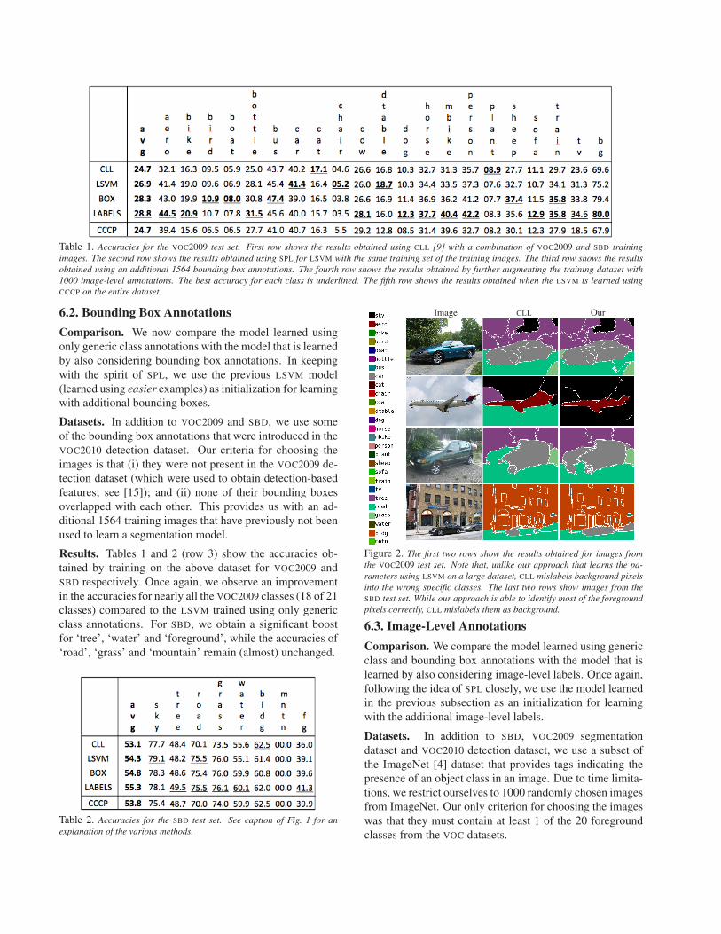
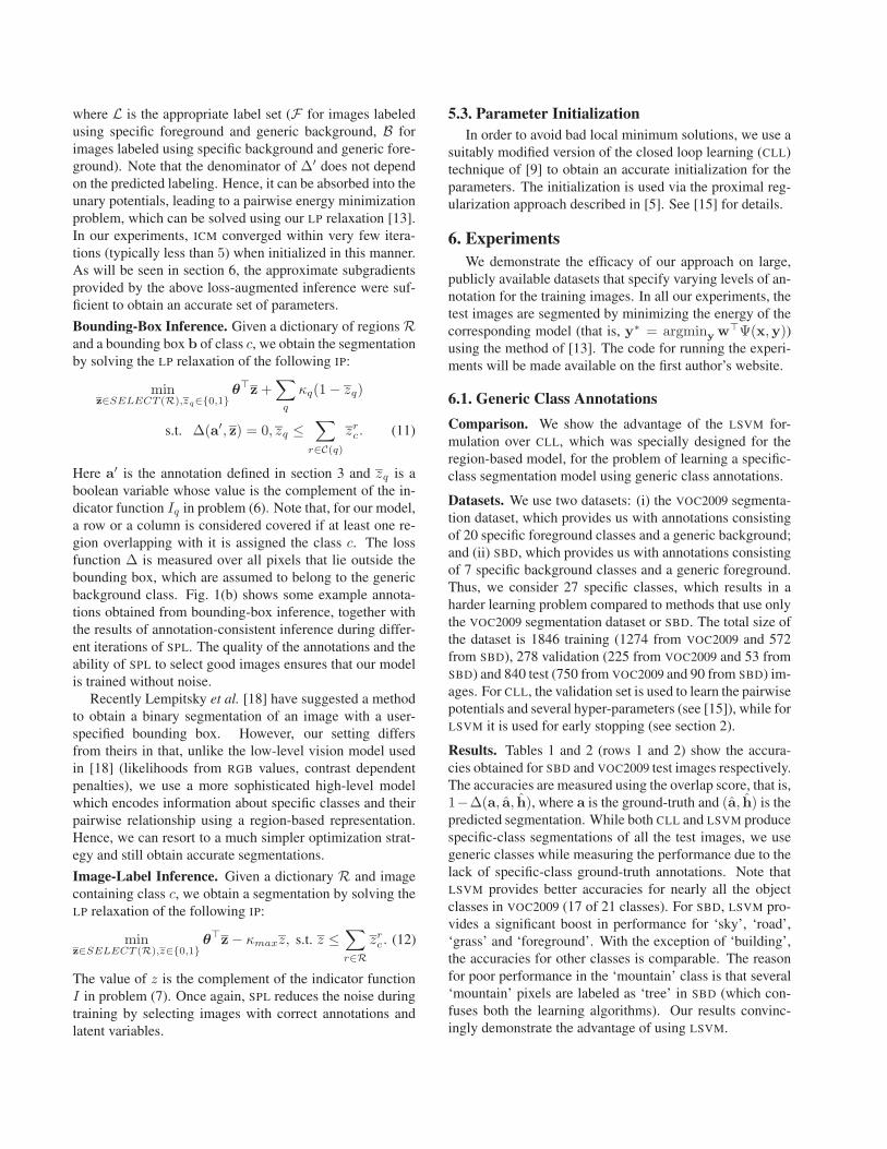
Table 1. Accuracies for the VOC2009 test set. First row shows the results obtained using CLL [9] with a combination of VOC2009 and SBD training

images. The second row shows the results obtained using SPL for LSVM with the same training set of the training images. The third row shows the results

obtained using an additional 1564 bounding box annotations. The fourth row shows the results obtained by further augmenting the training dataset with

1000 image-level annotations. The best accuracy for each class is underlined. The fifth row shows the results obtained when the LSVM is learned using

CCCP on the entire dataset.

6.2. Bounding Box Annotations

Comparison. We now compare the model learned using

only generic class annotations with the model that is learned

by also considering bounding box annotations. In keeping

with the spirit of SPL, we use the previous LSVM model

(learned using easier examples) as initialization for learning

with additional bounding boxes.

Datasets. In addition to VOC2009 and SBD, we use some

of the bounding box annotations that were introduced in the

VOC2010 detection dataset. Our criteria for choosing the

images is that (i) they were not present in the VOC2009 de-

tection dataset (which were used to obtain detection-based

features; see [15]); and (ii) none of their bounding boxes

overlapped with each other. This provides us with an ad-

ditional 1564 training images that have previously not been

used to learn a segmentation model.

Results. Tables 1 and 2 (row 3) show the accuracies ob-

tained by training on the above dataset for VOC2009 and

SBD respectively. Once again, we observe an improvement

in the accuracies for nearly all the VOC2009 classes (18 of 21

classes) compared to the LSVM trained using only generic

class annotations. For SBD, we obtain a significant boost

for ‘tree’, ‘water’ and ‘foreground’, while the accuracies of

‘road’, ‘grass’ and ‘mountain’ remain (almost) unchanged.

Table 2. Accuracies for the SBD test set. See caption of Fig. 1 for an

explanation of the various methods.

Image CLL Our

Figure 2. The first two rows show the results obtained for images from

the VOC2009 test set. Note that, unlike our approach that learns the pa-

rameters using LSVM on a large dataset, CLL mislabels background pixels

into the wrong specific classes. The last two rows show images from the

SBD test set. While our approach is able to identify most of the foreground

pixels correctly, CLL mislabels them as background.

6.3. Image­Level Annotations

Comparison. We compare the model learned using generic

class and bounding box annotations with the model that is

learned by also considering image-level labels. Once again,

following the idea of SPL closely, we use the model learned

in the previous subsection as an initialization for learning

with the additional image-level labels.

Datasets. In addition to SBD, VOC2009 segmentation

dataset and VOC2010 detection dataset, we use a subset of

the ImageNet [4] dataset that provides tags indicating the

presence of an object class in an image. Due to time limita-

tions, we restrict ourselves to 1000 randomly chosen images

from ImageNet. Our only criterion for choosing the images

was that they must contain at least 1 of the 20 foreground

classes from the VOC datasets.

Results. Tables 1 and 2 (row 4) show the accuracies ob-

tained by training on the above dataset for VOC2009 and

SBD respectively. For the VOC2009 segmentation test set,

the final model learned from all the training images provides

the best accuracy for 12 of the 21 classes. Compared to

the model learned using generic class labels and bounding

boxes, we obtain a significant improvement for 13 classes

by incorporating image-level annotations. Of the remaining

8 classes, the accuracies are comparable for ‘bird’, ‘boat’,

‘chair’ and ‘train’. For the SBD test set, the model trained

using all the data obtains the highest accuracy for 5 of the

8 classes. Fig. 2 shows examples of the specific-class seg-

mentation obtained using our method. Note that the param-

eters learned using our approach on a large dataset are able

to correctly identify the specific classes of pixels.

6.4. SPL vs. CCCP

Comparison. We now test the hypothesis that our SPL al-

gorithm is better suited for learning with diverse data than

the previously used CCCP algorithm.

Datasets. We use the entire dataset consisting of strongly

supervised images from the SBD and VOC2009 segmentation

datasets and weakly supervised images from the ImageNet

and VOC2010 detection datasets.

Results. Tables 1 and 2 (row 5) show the accuracies ob-

tained using CCCP for VOC2009 and SBD respectively. Note

that CCCP does not provide any improvement over CLL,

which is trained using only the strongly supervised images,

in terms of the average overlap score for VOC2009 . While

the overlap score improves for the SBD dataset, the improve-

ment is significantly better when using SPL (row 4). These

results convincingly demonstrate that, unlike CCCP, SPL is

able to handle the noise inherent in the problem of learning

with diverse data.

7. DiscussionWe presented a principled LSVM framework for learning

specific-class segmentation using diverse data, and convinc-

ingly demonstrated its benefits using large, publicly avail-

able datasets. While we focused on only three types of

annotations, our method can be extended to handle other

types of data. For example, instead of just a two-level hier-

archy (the generic classes and the specific classes), we can

consider a general hierarchy of labels, such as the one de-

fined in ImageNet [4] ( ‘Ferrari’ and ‘Honda’ sub-classes

for ‘car’). Such a hierarchy can be viewed as a tree over

labels. Given a pixel p annotated with a non-leaf label l,

we can specify a latent variable hp that models its leaf-level

label (where the leaves are restricted to lie in the sub-tree

rooted at l). The loss function and the inference algorithms

for generic classes can be trivially modified to deal with this

more general case.

Our ongoing work is in two directions: (i) dealing with

noisy labels, such as the labels obtained from Google Im-

ages or Flickr; and (ii) improving the efficiency of SPL by

exploiting the fact that very easy images can be discarded

during later iterations. Both these directions are aimed to-

wards learning a segmentation model from the millions of

freely available images on the Internet.

Acknowledgements. This work is supported by NSF under

grant IIS 0917151, MURI contract N000140710747, and

the Boeing company.

References

[1] B. Alexe, T. Deselaers, and V. Ferrari. ClassCut for unsupervised

class segmentation. In ECCV, 2010.

[2] H. Arora, N. Loeff, D. Forsyth, and N. Ahuja. Unsupervised seg-

mentation of objects using efficient learning. In CVPR, 2007.

[3] L. Cao and L. Fei-Fei. Spatially coherent latent topic model for

concurrent segmentation and classification of objects and scene. In

ICCV, 2007.

[4] J. Deng, W. Dong, R. Socher, L.-J. Li, K. Li, and L. Fei-Fei. Ima-

geNet: A large-scale hierarhical image database. In CVPR, 2009.

[5] C. Do, Q. Le, and C.-S. Foo. Proximal regularization for online and

batch learning. In ICML, 2009.

[6] M. Everingham, L. Van Gool, C. Williams, J. Winn, and A. Zisser-

man. The PASCAL visual object classes (VOC) challenge. IJCV,

2010.

[7] P. Felzenszwalb, D. McAllester, and D. Ramanan. A discriminatively

trained, multiscale, deformable part model. In CVPR, 2008.

[8] J. Gonfaus, X. Boix, J. Van de Weijer, A. Bagdanov, J. Serrat, and

J. Gonzalez. Harmony potentials for joint classification and segmen-

tation. In CVPR, 2010.

[9] S. Gould, R. Fulton, and D. Koller. Decomposing a scene into geo-

metric and semantically consistent regions. In ICCV, 2009.

[10] X. He, R. Zemel, and M. Carriera-Perpinan. Multiscale conditional

random fields for image labeling. In CVPR, 2004.

[11] N. Komodakis and N. Paragios. Beyond pairwise energies: Efficient

optmization for higher-order MRFs. In CVPR, 2009.

[12] S. Konishi and A. Yuille. Statistical cues for domain specific image

segmentation with performance analysis. In CVPR, 2000.

[13] M. P. Kumar and D. Koller. Efficiently selecting regions for scene

understanding. In CVPR, 2010.

[14] M. P. Kumar, B. Packer, and D. Koller. Self-paced learning for latent

variable models. In NIPS, 2010.

[15] M. P. Kumar, H. Turki, D. Preston, and D. Koller. Learning specific-

class segmentation from diverse data. Technical report, Stanford Uni-

versity, 2011.

[16] L. Ladicky, C. Russell, P. Kohli, and P. Torr. Associative hierarchical

CRFs for object class image segmentation. In ICCV, 2009.

[17] D. Larlus and F. Jurie. Combining appearance models and Markov

random fields for category level object segmentations. In CVPR,

2008.

[18] V. Lempitsky, P. Kohli, C. Rother, and T. Sharp. Image segmentation

with a bounding box prior. In ICCV, 2009.

[19] F. Li, J. Carreira, and C. Sminchisescu. Object recognition as ranking

holistic figure-ground hypotheses. In CVPR, 2010.

[20] S. Shalev-Shwartz, Y. Singer, and N. Srebro. Pegasos: Primal esti-

mated sub-gradient solver for SVM. In ICML, 2009.

[21] J. Shotton, J. Winn, C. Rother, and A. Criminisi. TextonBoost: Joint

appearance, shape and context modeling for multi-class object recog-

nition and segmentation. In ECCV, 2006.

[22] J. Winn and N. Jojic. LOCUS: Learning object classes with unsuper-

vised segmentation. In ICCV, 2005.

[23] Y. Yang, S. Hallman, D. Ramanan, and C. Fowlkes. Layered object

detection for multi-class segmentation. In CVPR, 2010.

[24] C.-N. Yu and T. Joachims. Learning structural SVMs with latent

variables. In ICML, 2009.