Learning Shape, Motion and Elastic Models in Force Space

Antonio Agudo1 Francesc Moreno-Noguer21Instituto de Investigacion en Ingenierıa de Aragon (I3A), Universidad de Zaragoza, Spain

2Institut de Robotica i Informatica Industrial (CSIC-UPC), Barcelona, Spain

Abstract

In this paper, we address the problem of simultaneouslyrecovering the 3D shape and pose of a deformable and po-tentially elastic object from 2D motion. This is a highly am-biguous problem typically tackled by using low-rank shapeand trajectory constraints. We show that formulating theproblem in terms of a low-rank force space that induces thedeformation, allows for a better physical interpretation ofthe resulting priors and a more accurate representation ofthe actual object’s behavior. However, this comes at theprice of, besides force and pose, having to estimate the elas-tic model of the object. For this, we use an ExpectationMaximization strategy, where each of these parameters aresuccessively learned within partial M-steps, while robustlydealing with missing observations. We thoroughly validatethe approach on both mocap and real sequences, showingmore accurate 3D reconstructions than state-of-the-art, andadditionally providing an estimate of the full elastic modelwith no a priori information.

1. IntroductionThe goal of the Non-Rigid Structure from motion

(NRSfM) is to simultaneously recover the camera motionand 3D shape of a deformable object from monocularimages. It is known to be a severely under-constrainedproblem, typically solved by introducing prior informa-tion through shape deformation models or camera trajectoryconstraints. Along these lines, early approaches extendedthe rigid factorization algorithm [37] to the non-rigid do-main [7, 12, 39], and approximated the shape by a linearcombination of basis estimated on-the-fly. Alternatively,other approaches have represented the evolution over timeof each point on the object through a set of pre-defined tra-jectory basis [6, 29, 41]. Both these constraints are com-monly referred to as statistical priors, as they do not have adirect physical interpretation.

In this paper, we introduce a new constraint based on alow-rank force prior. This prior has a direct physical in-terpretation, as it models the interaction between the object

Figure 1. Low-rank force space. Non-rigid shape can be repre-sented by means of the object elastic model and the force fieldacting on it. In turn, the full force field can be approximated by alow-rank basis. In this work, we simultaneously learn the elasticmodel (compliance matrix) and estimate the low-rank force space,while recovering shape and camera motion. In the figure we repre-sent the full force-space and its corresponding shapes in red. Thelow-rank forces and shapes are shown in blue.

and the underlying forces that deform it. Interestingly, wealso show its connection with the aforementioned shape andtrajectory models, turning these, into physical priors too.

The essence of our approach is described in Fig. 1. Letus consider N points on the object, which is deformed un-der the action of external forces. Following continuum me-chanics, the relation between the acting forces and the de-formation field can be characterized by an elastic model.Regarding the force space, we can fully define it by 3N in-dependent forces, whose combination allows mapping theshape from a rest configuration to a wide variety of arbitraryarrangements. Yet, to represent realistic deformations, onlya few of these forces, conforming a low-rank force space,are necessary. Based on this idea, we propose a new for-mulation of the NRSfM problem in which, given 2D pointtracks, we estimate camera trajectory and force parameters(and consequently shape). Even though reasoning on theforce space introduces the compliance matrix as new un-known, we are able to simultaneously solve for all parame-ters using Expectation Maximization (EM), with partialM -steps. By thorough testing on mocap and real sequences we

1

show that our formulation yields more accurate reconstruc-tions than state-of-the-art shape and trajectory based meth-ods, while providing more physical insights in terms of theelastic model of the object.

2. Related Work

The inherent ambiguity of the NRSfM problem is com-monly tackled by constraining the shape to lie on a low-rankspace spanned by a set of deformation modes [7, 16, 17, 39].This is further constrained by enforcing spatial [39] ortemporal [7, 17] shape smoothness, or by imposing the3D shapes to be closely aligned [22]. A number of ap-proaches, instead constraining the shape, introduce restric-tions on the trajectory of every object point using predefinedbases [6, 29, 41]. There have also been recent attempts tocombine low-rank shape and trajectory spaces [19, 20, 35].All these techniques are referred to as statistically-basedmethods, since the low-rank representations used to con-dition the problem are not physically grounded. Despitetheir popularity, one inherent limitation of these methods isthat they are very sensitive to the number of shape or trajec-tory modes, which needs to be carefully chosen to correctlymodel the deformation.

A better representation of the underlying dynamics in-volved in non-rigid deformations can be obtained throughphysically-grounded models [26, 34]. Force-based kine-matics [4, 13, 33], linear elastic models [24], and numer-ical techniques based on Finite Element Methods (FEM)for tracking [43] or 3D reconstruction [2], are just a fewexamples of the renewed interest in physical models. Ad-ditionally, there exist approaches in which the parametersruling these models are learned from input data. For in-stance, displacement and force measurements allow recov-ering the Young’s modulus [44] together with the Poisson’sratio [9]. More recently, material properties of fabrics mov-ing under wind forces [11] or under small motions [15] areestimated from only video sequences. And vice-versa, ap-plied forces can be recovered from 2D displacements and anestimate, up to scale, of the elastic parameters [2]. However,in all these approaches only small pieces of the full physicalmodel (i.e., the complete stiffness matrix) are recovered.

Contribution: In this paper we propose a new low-rankforce model which we use to simultaneously recover cam-era motion, 3D shape and the full elastic model of the object.Note that the latter is specially challenging, as it involves es-timating a large number of parameters, and not just the ma-terial properties such as the Young’s modulus or Poisson’sratio. We do all this from the sole input of 2D input tracks,which may even be discontinuous due to missing data. Inaddition, we link our physical model to previous shape andtrajectory statistical approaches, giving them a physical in-terpretation, too.

3. Low-rank Force ModelA standard approach to reduce the ambiguity of the

NRSfM problem involves representing the object in low di-mensional spaces. Two spaces have been considered so far,the shape and the trajectory ones. Before describing the newlow-rank force space we propose, we review these previousformulations.

3.1. Low-rank Shape and Trajectory Space

The most natural way to represent time-varying shapesis by means of a low-rank shape basis. These priorsare computed using either Principal Component Analysis(PCA) over training data [10, 27], applying modal analysisover a rest configuration [1, 30], or are estimated on-the-fly [12, 17, 28, 39]. In particular, let us consider N 3Dpoints on an object, being observed along T frames. If wedenote by xt

i = [xti, yti , z

ti ]> the 3D coordinates of the i-th

point at time t, and by st = [(xt1)>, . . . , (xt

N )>]> the 3N -dimensional representation of the shape at time t, we cancompactly write the time-varying shape as a 3N×T matrixS = [s1, . . . , sT ]. Every instant shape st can be approxi-mated by a linear combination or Q basis shapes sq:

st =

Q∑q=1

ψtq sq = Sψt (1)

where ψt = [ψt1, . . . , ψ

tQ]> are the coefficients for the

shape at time t, and S = [s1, . . . , sQ] is a 3N×Q matrixcontaining all basis shapes. By aggregating all coefficientsinto a Q×T matrix Ψ = [ψ1, . . . ,ψT ], we can finally writethe factorization of the time-varying shape S as:

S = SΨ. (2)

Alternatively, we could include a shape at rest s0 in the sub-set of basis shapes [1, 39]. In that case, we would takeS = [s0, s1, . . . , sQ], and the basis vectors si, i = 1, . . . , Qwould be interpreted as 3D displacements over s0.

When representing the time-varying structure in trajec-tory space [6], predefined basis of a Discrete Cosine Trans-form (DCT) are used to span the trajectory of each objectpoint (i.e., the rows of S). We can then factorize S as:

S = ΦT, (3)

where T is a Q×T matrix made of Q predefined basis tra-jectories, and Φ is a 3N×Qmatrix of trajectory coefficients.

3.2. Modeling Shapes in a Low-rank Force Space

We next derive the formulation of our physics-basedlow-rank force model to represent the shape. We draw inspi-ration on the Hooke’s law, which states that the force neededto extend or compress a spring by a certain distance is pro-portional to that distance by a factor k, known as stiffness.

This simple model can be generalized to 3D objects withmass and volume, resulting in complex systems of partialdifferential equations [8] that generally do not have an ana-lytical solution and require from numerical approximations,such as FEM. For instance, applying FEM over a shape atrest, made ofN points and represented as a 3N-dimensionalvector s0, yields the following linear system:

Ku = f , (4)

where K is the 3N×3N stiffness matrix that maps the 3Ndisplacement vector u into a 3N -dimensional force fieldf . The matrix K is usually built considering a number ofphysical characteristics, such as material elastic properties,the type of deformation (e.g., beam bending, stress plane)and the connectivity between the nodal points, which de-pends on the type of element discretization (e.g., triangular,wedge, tetrahedral). Additionally, unless providing bound-ary conditions, K is ill-conditioned, i.e., rank(K) < 3N .

Note that Eq. (4) allows computing the forces f that needto be applied onto every point of s0 to obtain a pre-defineddisplacement u. However, we will regard this relation inthe opposite direction, that is, we seek to compute the 3Ddisplacement when the 3D acting forces are known. In thiscase, we will apply the relation u = Cf , where C is a3N × 3N compliance matrix. When boundary conditionsare known this matrix is computed as C = K−1 [5, 40], andC is guaranteed to be a strictly positive-definite symmetricmatrix. When boundary conditions are not available, wemake use of the pseudoinverse, i.e., C = K†, but we canonly assume C to be symmetric [2].

Once C is known, we can estimate a 3D displacementu for any 3D applied force vector f , and therefore a newconfiguration of the object shape as:

s = s0 + u = s0 + Cf = C(Ks0 + f) = C(f0 + f), (5)

where f0 = Ks0 can be interpreted as the forces applied tokeep the shape at rest. We can now expand this expressionto account for all T frames of a time-varying sequence:

S = C[f0 + f1, . . . , f0 + fT ] = CF, (6)

where F is a 3N×T matrix made of the force fields alongthe sequence. At this point we can introduce our low-rankforce model. As it has been previously done for the shapesor point trajectories, realistic distributions of acting forcescan also be approximated by a reduced number of modes.To follow the parallelism with the previous section, we con-sider a basis made of Q force vectors, and represent ourlow-rank force field as a 3N×Qmatrix F. The time-varyingshape can then be written as:

S = CFΓ, (7)

where Γ = [γ1, . . . ,γT ] is a Q×T matrix of time-varyingforce coefficients.

3.3. Shape-Trajectory-Force Duality

A direct comparison of the low-rank shape, trajectoryand force models defined in Equations (2), (3) and (7), re-spectively, gives the equivalence between the three repre-sentations. And most importantly, it gives a relation be-tween two models, the shape and trajectory ones, that havethus far been considered as statistical, and our new low-rankforce model, directly derived from physical relations.

In particular, considering the shape-force duality, we ob-serve that S = CF, that is, we can write the linear sub-space of shapes in terms of force and elasticity parameters,and therefore, the statistical shape model does inherentlyencode physically-grounded properties. Similarly, we canestablish a trajectory-force duality, and write that Φ = CFand T = Γ. In this case, the low-rank force model is equiv-alent to the trajectory coefficients, and the low-rank trajec-tory bases, correspond to the force coefficients.

It is also worth to point that while the proposed approachhas equal compaction power than shape and trajectory mod-els, factorizing the low-rank space into a force componentF, and a component C which encodes the elastic propertiesof the object, makes it possible to model a much wider rangeof object behaviors and configurations. This factorization,though, introduces an additional complexity in the learningprocess, as we need to discover all these terms from the soleinput of 2D tracks. In the next section, we describe how weresolve this learning process, but when this is done, besidesestimating shape, we could also address the inverse prob-lem of estimating the forces necessary to obtain a specificshape configuration. This might be extremely useful in cer-tain robotic applications dealing with the manipulation ofdeformable objects, or in laparoscopy surgery.

4. Learning Elastic Model, Shape and Pose

In this section we describe how we introduce our low-rank force space into the formulation of the NRSfM problem,and how we then simultaneously solve for the elastic modelof the object, plus the shape and camera pose.

4.1. Problem Formulation

Let us consider a deformable object with N points at atime instant t, represented by a 3N vector st. Assuming anorthographic camera model, we can write the projection ofthe 3D points onto the image plane as a 2N vector wt:

wt = Gtst + ht + nt, (8)

where Gt = IN ⊗ Rt has 2N× 3N size, IN is the N -dimensional identity matrix, Rt are the first two rows ofa full rotation matrix, and ⊗ denotes the Kronecker prod-uct. Similarly, ht = 1N ⊗ tt is a 2N vector resulting fromconcatenating N bidimensional translation vectors tt, and

Factor Full Shape Trajectory ForceCamera 5T 5T 5T 5TBasis - 3NQ - 3NQCoefficients - QT 3NQ QTModel 3NT - - 3N(3N + 1)/2

Total number 5T 5T + 3NQ 5T 5T + 3NQ+QTof unknowns +3NT +QT +3NQ +3N(3N + 1)/2

Table 1. Total number of unknowns that need to be estimated whenconsidering the Full model, or the low-rank models in Shape, Tra-jectory or Force space, respectively. The results are represented interms of the number of object points N , the number of frames Tand the dimensionality Q of the low-rank space.

1N is a N -vector of ones. Finally, nt is a 2N dimensionalvector of Gaussian noise.

We can therefore define our problem as that of estimat-ing, for t = 1, . . . , T , the shape st and camera pose pa-rameters {Rt, tt}, given the observation of point tracks wt

corrupted by noise nt. The total number of unobservedvariables includes 3NT parameters for the shape and 5Tparameters for the pose1. Estimating all these unknownsfrom the only 2NT noisy observations of the point tracksis clearly an ill-posed problem. We make the problemtractable by introducing our low-rank force model and en-coding the time-varying shape as:

st = s0 + ut = s0 + CFγt, (9)

where C is the compliance matrix, F are the low-rank forcevectors, and γt are the corresponding force coefficients atframe t. The projection Eq. (8) becomes:

wt = Gt(s0 + CFγt) + ht + nt. (10)

Note that using the low-rank force model introduces anew challenge to the problem, which is that besides hav-ing to estimate the variables involved in a standard NRSfMproblem (i.e., pose, shape basis and shape coefficients, orequivalently in our framework, pose, force basis and forcecoefficients), we now need to learn the full elastic model Cof the object.

Since C remains constant along the sequence, it intro-duces a fixed number of unknowns independently of thenumber of frames T . Specifically, C is a 3N× 3N sym-metric matrix, for which we only need to estimate the uppertriangular part, i.e., 3N(3N + 1)/2 elements. Addition-ally, we still need to estimate the 5T pose parameters, 3NQcomponents for the low-rank force space (assuming we con-sider a force basis with Q components), and QT unknownsfor the force coefficients. In Table 1 we summarize the to-tal number of unknowns as a function of the parameters N(number of points), T (number of frames) and Q (dimen-sionality of the low-rank space) and for the full-space prob-lem and the three low-rank versions (shape, trajectory and

1An orthographic projection has five degrees of freedom, namely thethree parameters describing the rotation matrix, plus two of the translation.

N T Q Obs. Full Shape Traj. Force55 260 12 28,600 44,200 6,400 3,280 20,09540 316 11 25,280 39,500 6,376 2,900 13,63629 450 7 26,100 41,400 6,009 2,859 9,83741 1,102 10 90,364 141,056 17,760 6,740 25,386

Table 2. Total number of unknowns that need to be estimated whenconsidering the Full model, or the low-rank models in Shape, Tra-jectory or Force space, respectively, for the combination of param-eters N , Q and T we consider in the experimental section. Thecolumn “Obs.” refers to the number of observed variables, 2NT ,corresponding to the 2D tracks of all N points along the T frames.

force). In Table 2 we give the number of unknowns for thespecific combinations of N , Q and T we will use in theexperimental section. Observe that for long sequences (Tlarge), the number of unknowns of the Shape and Force sub-spaces become similar, while our Force-based model yieldsmuch richer information about the elastic object properties.

4.2. Probabilistic Low-Rank Force Model

In order to simultaneously learn shape, pose and elas-tic models from 2D point tracks as described in Eq. (10),we follow a Probabilistic PCA formulation [31, 36, 38].Broadly, this consists of two main steps. We start by writingthe observations wt as a probabilistic distribution and thenwe estimate the parameters that maximize its likelihood us-ing EM. We next describe the first of these steps.

To estimate the distribution over the projected points wt

we first assume the weight coefficients γt to be modeled bya zero-mean Gaussian distribution γt ∼ N (0; IQ). Theseweights become latent variables that can be marginalizedout and are never explicitly computed, and using Eq. (9), wecan propagate their distribution to the time-varying shapes,yielding st ∼ N

(s0;CFF>C>

).

By also assuming the noise over the shape observationsnt to follow a Gaussian distribution with variance σ2, i.e.,nt ∼ N

(0;σ2I2N

), we can finally estimate that the pro-

jected points wt are also Gaussian:

wt ∼ N(Gts0 + ht;GtCF(GtCF)> + σ2I2N

)(11)

We next explain how we perform Maximum Likelihood Es-timation (MLE) on this latent variable problem using EM.

4.3. Expectation Maximization

For the purpose of estimating the MLE of the distributionin Eq. (11), we use an EM algorithm in a similar way asdone in [3, 38]. We denote by Θt ≡ {Rt, tt} the set ofmodel parameters to estimate per frame, Υ ≡ {C, F, σ2}the set of parameters to estimate along the sequence, γt thelatent variables and wt the observed data. Given the 2Dtrajectories of all points w = {w1, . . . ,wT }, we seek toestimate all set of parameters Θ = {Θ1, . . . ,ΘT ,Υ}. The

EM algorithm iteratively estimates the maximum likelihoodalternating between E-step and M -step.

4.3.1 E-StepWe initially estimate the posterior distribution over the la-tent variables given the current observations and model pa-rameters. Assuming iid samples and applying the Bayes’rule and the Woodbury’s matrix identity, it can be shownthis distribution to be:

p(γt|wt,Θt,Υ) ∼ N (µtγ ;Σ

tγ), (12)

where:

µtγ =Λ(wt −Gts0 − ht) ; Σt

γ = IQ −ΛGtCF

Λ =F>C(Gt)>

(σ2I2N + GtCF(GtCF)>)−1.

4.3.2 M-StepWe then replace the latent variables by their expected valuesand update the model parameters by optimizing the negativelog-likelihood functionA(Θ,w) with respect to the param-eters Θt, for t = 1, . . . , T , and Υ where:

A(Θ,w) = E

[−

T∑t=1

log p(wt|Θt,Υ)

]= NT log(2πσ2)

+1

2σ2

T∑t=1

E[‖wt −Gt(s0 −CFγt)− ht‖22

](13)

Note that this log-likelihood function is quadratic in allparameters we seek to estimate, and in contrast to [17,32, 33], it does not need regularization weights. To up-date every parameter, we compute the corresponding par-tial derivative assuming the other parameters are fixed, setit to zero and solve it. The update rules we obtain are thefollowing.

Updating Elastic Model (C): To perform computationswith the matrix C we need to rewrite it in vectorized form.Further, since C is symmetric, we only need to vectorize theupper triangular part of it. For this, we define the functionvech(·), a generalization of the full-matrix vectorization op-erator vec(·). The two operators can be related by means ofa so-called duplication matrix D, of size r2× r(r+1)

2 , wherer is the size of the original matrix we are vectorizing [23].For C, we have that r = 3N and we can write:

vec(C) = Dvech(C) . (14)

The inverse mapping is computed by means of the pseu-doinverse, that is, vech(C) = D†vec(C). If we now set∂A/∂vech(C) = 0, it can be shown that:

vech(C)←

(T∑

t=1

((Fµt

γ)>⊗ (D>(Fµt

γ ⊗ Ir)(Gt)>Gt)

)D

)−1

×T∑

t=1

D>(Fµtγ ⊗ Ir)(G

t)>(wt −Gts0 − ht).

Updating Low-Rank Force Space (F): For computing Fwe need to define the expectation φt

γγ = E[γt(γt)>] =

Σtγ + µt

γ(µtγ)>. By using again the vectorized form, we

can update the force space as:

vec(F)←

(T∑

t=1

(φtγγ)> ⊗ (GtC)>GtC

)−1

× vec

(T∑

t=1

(GtC)>(wt −Gts0 − ht)(µtγ)>

).

Updating the Camera Pose (Rt, tt): The camera rota-tion Rt needs to be updated enforcing orthonormality con-straints. In order to do so we follow the iterative strategyproposed in [3], where ∂A(Rt)/∂Rt = 0 is optimized en-forcing Rt to lie on the smooth manifold defined by theorthogonal group SO(3). Regarding the translation vectortt it is easy to show that it can be updated as:

tt ← 1

N

N∑i=1

(wti −Rt(s0,i + (CFµt

γ)i)), (15)

where wt = [(wt1)>, . . . , (wt

N )>]>, wi are 2D coordi-nates, s0 = [s>0,1, . . . , s

>0,N ]>, s0,i are 3D coordinates, and

(CFµtγ)i is the i-th 3D point of the 3N vector CFµt

γ .

Updating Noise Variance (σ2): Setting ∂A(σ2)/∂σ2 = 0we can finally update the noise variance as:

σ2 ← 1

2NT

T∑t=1

(tr((GtCF)>GtCFφt

γγ

)(16)

+‖wt−Gts0−ht‖2−2(wt−Gts0−ht

)>GtCFµt

γ

).

4.4. A Comment on Scale Factor

When solving for C and F we have only constrained Cto be symmetric. Therefore, we could consider any sym-metric and invertible matrix A such that CF = CAA−1F.A new compliance matrix CA would still be symmetric andwould yield the same solution for the shape reconstructionin Eq. (9) and reprojection in Eq. (10). That is, the values ofC and F are retrieved up to a scale factor matrix. A similarambiguity is produced between F and γt.

Nevertheless, the up to scale compliance matrix C, be-sides yielding a correct solution to the NRSfM problem, itis also sufficient to model the full physical space. We cantherefore use C to generate, up to scale, any deformationu applying a given force vector f . And vice-versa, we canobtain an scaled force field to produce a specific displace-ment. This kind of physical relations, are of course, notpossible with previous low-rank shape and trajectory ap-proaches. What is not possible with the compliance matrixwe retrieve, though, is to directly estimate the ground truth

Space: Shape Trajectory Shape-Trajectory ForcePPPPPPPPSeq.

Met.EM-PPCA [39] EM-LDS [39] MP [28] SPM [14] EM-PND [22] PTA [6] CSF2 [20] KSTA [19] EM-PFS

Jacky [39] 1.80(5) 2.79(2) 2.74(5) 1.82(7) 1.41 2.69(3) 1.93(5) 2.12(4) 1.80(7)Face [28] 7.30(9) 6.67(2) 3.77(7) 2.67(9) 25.79 5.79(2) 6.34(5) 6.14(8) 2.85(5)Flag 4.22(12) 6.34(3) 10.72(3) 7.84(5) 4.11 8.12(6) 7.96(2) 7.74(2) 5.29(12)Walking [39] 11.11(10) 27.29(2) 17.51(3) 8.02(6) 3.90 23.60(2) 6.39(5) 6.36(5) 8.54(11)Average error: 6.11 10.77 8.69 5.09 8.80 10.05 5.66 5.59 4.62

Table 3. Quantitative comparison on Mocap videos. We report e3D[%] for shape basis methods EM-PPCA [39], EM-LDS [39], MP [28]and SPM [14]; for EM-PND [22]; for the trajectory basis method PTA [6]; for shape-trajectory basis methods CSF2 [20] and KSTA [19];and for our force basis approach denoted as EM-PFS. We have chosen the basis rank (in brackets) that gave the lowest e3D error.

values of the inherent physical parameters (e.g., Poisson’sratio or Young’s modulus) that constitute the true stiffnessmatrix. For this to be possible we should perform a calibra-tion and estimate the actual scale factor matrix, in the sameline as [21] did for very specific force sensors.

4.5. Dealing with Missing Data

Unlike other methods [12, 14], our approach can easilyincorporate an strategy to handle incomplete measurementsdue to occlusions or outliers. To achieve this, during theM -step of EM algorithm, we just need to optimize the expectedlog-likelihoood of the 2D location wt

i of the missing points.Since we are using a global model, we can infer their value,despite not being available. In particular we set them to:

wti ← Rt(s0,i + (CFµt

γ)i) + tt. (17)

4.6. Initialization

The optimization of Eq. (13) is a highly non-linear prob-lem involving a large number of parameters. For this,it is important not to initialize them completely at ran-dom. In particular, we initialize the rigid motion parame-ters {Rt, tt} and s0 considering the scene does not deform,and we apply rigid factorization [25] as standard practicein NRSfM techniques. Regarding the compliance matrix C,we do not use any physical prior, and initially set it to theidentity matrix. The force basis F is initialized through acoarse-to-fine approach, in which a noise-free version ofEq. (10), where all parameters except F are given, is firstsolved for one force-mode, then for two modes, and so onuntil estimating the Q initial modes. Once all these param-eters are set, the starting value of σ2 is directly computedfrom Eq. (16). Finally, when dealing with missing data weassume that both the camera motion and 3D shape deforma-tion are smooth over time, and obtain an initial estimationof the missing tracks wt

i by imposing smooth trajectories,as done in [20].

5. Experimental EvaluationWe now present our experimental results for different

types of sequences including articulated and non-rigid mo-tion (see videos in the supplemental material). We provide

both qualitative and quantitative results, where we compareour approach against state-of-the-art methods, using severalmocap datasets with 3D ground truth. For these datasetswe report the standard 3D reconstruction error, computedas e3D = 1

T

∑Tt=1

‖st−stGT ‖F‖stGT ‖F

, where ‖ · ‖F denotes theFrobenius norm, st is the estimated 3D reconstruction andstGT is the corresponding 3D ground truth. e3D is computedafter aligning the estimated 3D shape with the 3D groundtruth using Procrustes analysis over all T frames.

5.1. Motion Capture Data

The standard way to compare NRSfM approaches isthrough a number of datasets with ground truth, acquiredusing mocap systems. We consider the following ones: theface deformation sequences Jacky and Face, from [39] and[28], respectively; Walking for articulated motion from [39],and a sparse version of Flag waving in the wind [42].

We compare our approach, denoted EM-PFS (forExpectation-Maximization on Probabilistic Force Space)against eight other methods, which use low-rank models onboth shape and trajectory spaces. Among the shape spacemethods we consider: EM-PPCA [39], EM-LDS [39], theMetric Projections (MP) [28], the block matrix approachfor SPM [14] and EM-PND [22]. Regarding the trajectory-based ones, we evaluate the DCT-based 3D point trajectory(PTA) [6]. As shape-trajectory methods we consider Col-umn Space Fitting (CSF2) [20] and the Kernel Shape Tra-jectory Approach (KSTA) [19]. The parameters of thesemethods were set in accordance with their original pa-pers. In our approach, the only parameter that needs tobe manually set is the number Q of modes of the low-rankforce space. There is no other parameter nor regularizationweight that needs to be tuned.

The mean 3D reconstruction errors are summarized inTable 3. Observe that our approach consistently performseither the best or among the best in all sequences, and inaverage is the one with smaller error. In particular note thatwe slightly outperform SPM [14] and KSTA [19], which areacknowledged to be at the top of the state-of-the-art in low-rank based models. And most importantly, we do not onlysolve for the NRSfM problem, but we additionally providean estimation of the full elastic model of the object.

Figure 2. Actress sequence. Top: 2D tracking data (green circles)and reprojection (red dots) of the reconstructed 3D shape. Mid-dle: Camera and side-views of the reconstructed shapes. Bottom:Same views using EM-PND [22].

Figure 3. Beating heart sequence. Top: See caption of Fig. 2.Middle: Reconstructed 3D shape, color code such that reddishareas indicate larger displacements. Bottom: Reconstructed 3Dshape, using the original texture. Best viewed in color.

5.2. Real Videos

We have also evaluated our approach on several real se-quences, which despite not having ground truth, allow aqualitative evaluation in different real-world scenarios andunder the presence of structured occlusions, where other ap-proaches are prone to fail [14].

First, we process the actress sequence, with 102 framesshowing a woman talking and moving her head. The pointtracks were provided by [7]. Figure 2 shows the 3D recon-struction, appropriately rotated according to the estimatedpose. We also show the results of the EM-PND [22], knownto be very accurate except for situations like this sequence,in which the camera rotation is small.

For the beating heart sequence, of 79 frames and ac-quired during bypass surgery2, we use the outlier-free pointtracks of [18], computed using optical flow. Figure 3 showsthe 3D reconstruction we obtain, where one of the mainchallenges is that the movement of the camera is very small.This especially penalizes trajectory-based methods. Thecolor-coded reconstructions, representing the amount of de-formation, show that we can recover the rhythmic deforma-tions of the heart, while learning its elastic model.

2Sequence available from: http://hamlyn.doc.ic.ac.uk/vision

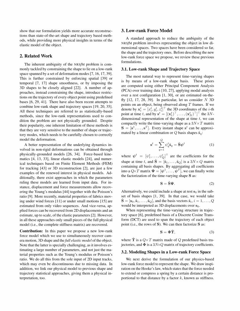
Figure 4. Back sequence. Top: See caption of Fig. 2. Bottom:Side view of the reconstructed shape.

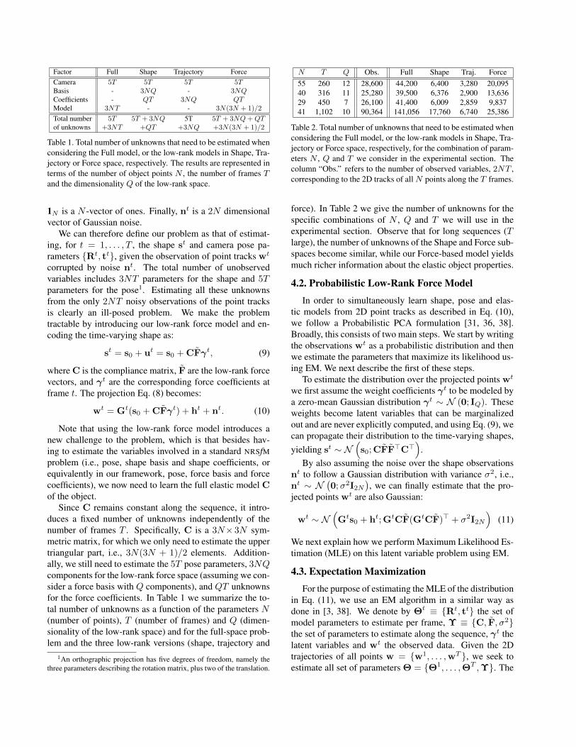
Figure 5. ASL sequence. Top: See caption of Fig. 2. Bottom:Camera frame and side-views of the reconstructed 3D shape. Bluecircles correspond to missing points. Best viewed in color.

Figure 4 shows the reconstruction of the back of a per-son. Point tracks are obtained from [32]. Again, one of thedifficulties of this sequence is to deal with small camera mo-tions, which our approach handles without much difficulty.

Finally, we have also processed an ASL sequence of anAmerican Sign Language (ASL), consisting of a personmoving the head while talking and hand gesturing. The goalis to reconstruct the face which, in some frames is partiallyoccluded by the hand or by the own face rotation. The se-quence, from [20], has 114 frames and 11.5% of missingdata. Fig. 5 shows two views per frame of the estimated 3Dshape. Note that even when occlusions appear, our modelprovides a correct estimation for the occluded shape. Whilethis reconstruction is very similar to that obtained by [20],SPM [14], our closer competitor in the mocap data experi-ments of Table 3, is not able to handle missing data.

5.3. Elastic Model Estimation

The distinguishing contribution of our approach is thatbesides estimating the shape and camera trajectory, we pro-vide an estimation of the elastic model of the object C, anda low-rank force space F (with the corresponding force co-efficients Γ). Additionally, as discussed in Sect. 3.3, oncewe have estimated these parameters, we can directly com-pute the equivalence between the force, shape and trajec-tory spaces. Concretely, the low-rank shape space has beenshown to be S = CF, and the low-rank trajectory spaceT = Γ. In Fig. 6 we plot these equivalences for the ex-ample of the actress sequence introduced previously. On

Forc

eSh

ape

Traj

ecto

ry

0 20 40 60 80 100−5

0

5

Number of frame t 0 20 40 60 80 100

−5

0

5

Number of frame t 0 20 40 60 80 100

−5

0

5

Number of frame t 0 20 40 60 80 100

−5

0

5

Number of frame t 0 20 40 60 80 100

−5

0

5

Number of frame t

Figure 6. Spaces comparison. Equivalence between the force,shape and trajectory spaces using the actress sequence, with rankQ = 5. Top: Modes in the force space. Middle: Modes in theshape space. Bottom: Modes in the trajectory space.

top we plot the first five force modes, as vectors overlay-ing the shape at rest. Observe that the larger magnitudes ofthe modes concentrate around the mouth, which is the partof the face undergoing larger deformations. On the cen-ter, we plot the equivalent shape basis we retrieve. Again,although it is difficult to appreciate from non-overlappingimages, note the subtle differences between the configura-tion of each mode, and again, particularly around the areaof the mouth. The bottom-most plot, depicts the first fivetrajectory modes, with size equal to the sequence length.The theoretical modes used in the trajectory-based methodscorrespond to the sinusoidal functions of a DCT. Note thatthe first mode we estimate from our force-space, quite re-sembles such a function.

In Fig. 7 we demonstrate that the compliance matrix weestimate allows recovering the full physical space. For in-stance the four face configurations we plot on the left areproduced by applying specific forces f and computing theresulting deformations u via the relation u = Cf . Eachface corresponds to the product of the compliance matrix,shown in the center of the figure, by one of the force vec-tors f1, f2, f3, f4 depicted on the right, plus the shape at rest.Observe that with this force model we can generate shapeconfigurations (e.g., winking one or two eyes, mouth wideopen) that would be hard or impossible to obtain using low-rank shape and trajectory spaces unless similar shapes areexplicitly observed (in shape-based methods) or they usea very large number of modes (in trajectory-based meth-ods). In contrast, using the physical space we propose, wecan produce these shapes even when they have not been ob-served and directly from the elastic model we have learned.Additionally, note how the forces f1, f2, f3, f4 necessary toproduce these shape configurations are smooth (their colorcoded components do not abruptly change). This wouldnot happen if we had used a random symmetric compli-

Degrees of freedom

De

gre

es

of

fre

ed

om

Full Physical Space (C)

0 50 100 150 200

0

20

40

60

80

100

120

140

160

180

200

f1

f2

f3

f4 f

1r f

2r f

3r f

4r

Figure 7. Full physical space estimation for the actress se-quence. Once the compliance matrix is learned, we can defineany shape in the full physical space. Left: Four shapes obtainedfrom the estimated C. Center: Recovered C. Right: f1, f2, f3, f4,are the forces necessary to obtain the shape configurations on theleft from C, the estimated compliance matrix. f r

1, fr2, f

r3, f

r4, are the

forces necessary to obtain the same shape configurations, but froma random symmetric compliance matrix. Best viewed in color.

ance matrix. This matrix would also solve allow minimiz-ing Eq. (13), but the resulting forces f r

1, fr2, f

r3, f

r4 would not

be quite realistic. We plot these forces, on the rightmostof Fig. 7. Note how their values evidence sharp changes,indicating that a random compliance matrix would not ap-propriately model the underlying physics of the object.

6. ConclusionsIn this paper we have formulated the NRSfM problem us-

ing a new low-rank force model. From only 2D point tracks,besides recovering shape and camera motion, this approachalso provides an estimation of an elastic model of the object,allowing for rich physical interpretations of the dynamicsin terms of force and displacement. Additionally, we haveshown the connections of our force-model to the shape andtrajectory-based spaces used so far. The results demonstratethat the proposed technique is applicable to a wide varietyof real-world deformations and materials, without requiringany prior knowledge about the physical or geometric ob-ject properties. We obtain state-of-the-art performance inreconstruction accuracy, while also providing an estimationof the object elastic model. Yet, this model is recovered upto scale. In the future, we plan to retrieve the true elasticmodel by including certain constraints into our optimiza-tion. By doing this from just a monocular video would be amajor step in engineering mechanics, which usually rely oncomplex laboratory procedures for obtaining such models.

AcknowledgmentsThis work was partly funded by the MINECO projects

DIP2012-32168 and TIN2014-58178-R; by the ERA-netCHISTERA project VISEN PCIN-2013-047; and by ascholarship FPU12/04886 of the Spanish MECD. We alsothank Paulo Gotardo for making their data available.

References[1] A. Agudo, L. Agapito, B. Calvo, and J. M. M. Montiel. Good

vibrations: A modal analysis approach for sequential non-rigid structure from motion. In CVPR, 2014.

[2] A. Agudo, B. Calvo, and J. M. M. Montiel. Finite elementbased sequential bayesian non-rigid structure from motion.In CVPR, 2012.

[3] A. Agudo, J. M. M. Montiel, L. Agapito, and B. Calvo. On-line dense non-rigid 3D shape and camera motion recovery.In BMVC, 2014.

[4] A. Agudo and F. Moreno-Noguer. Simultaneous pose andnon-rigid shape with particle dynamics. In CVPR, 2015.

[5] A. Agudo, F. Moreno-Noguer, B. Calvo, and J. M. M. Mon-tiel. Sequential non-rigid structure from motion using phys-ical priors. TPAMI, to appear, 2015.

[6] I. Akhter, Y. Sheikh, S. Khan, and T. Kanade. Non-rigidstructure from motion in trajectory space. In NIPS, 2008.

[7] A. Bartoli, V. Gay-Bellile, U. Castellani, J. Peyras, S. Olsen,and P. Sayd. Coarse-to-fine low-rank structure-from-motion.In CVPR, 2008.

[8] K. J. Bathe. Finite element procedures in Engineering Anal-ysis. Prentice-Hall, 1982.

[9] M. Becker and M. Teschner. Robust and efficient estima-tion of elasticity parameters using the linear finite elementmethod. In SIMVIS, 2007.

[10] V. Blanz and T. Vetter. A morphable model for the synthesisof 3D faces. In SIGGRAPH, 1999.

[11] K. L. Bouman, B. Xiao, P. Battaglia, and W. T. Freeman.Estimating the material properties of fabric from video. InICCV, 2013.

[12] C. Bregler, A. Hertzmann, and H. Biermann. Recoveringnon-rigid 3D shape from image streams. In CVPR, 2000.

[13] M. Brubaker, L. Sigal, and D. Fleet. Estimating contact dy-namics. In ICCV, 2009.

[14] Y. Dai, H. Li, and M. He. A simple prior-free method fornon-rigid structure from motion factorization. In CVPR,2012.

[15] A. Davis, K. Bouman, J. Chen, M. Rubinstein, F. Durand,and W. Freeman. Visual vibrometry: Estimating materialproperties from small motions in video. In CVPR, 2015.

[16] K. Fragkiadaki, M. Salas, P. Arbelaez, and J. Malik.Grouping-based low-rank trajectory completion and 3D re-construction. In NIPS, 2014.

[17] R. Garg, A. Roussos, and L. Agapito. Dense variational re-construction of non-rigid surfaces from monocular video. InCVPR, 2013.

[18] R. Garg, A. Roussos, and L. Agapito. A variational ap-proach to video registration with subspace constraints. IJCV,104(3):286–314, 2013.

[19] P. F. U. Gotardo and A. M. Martinez. Kernel non-rigid struc-ture from motion. In ICCV, 2011.

[20] P. F. U. Gotardo and A. M. Martinez. Non-rigid structurefrom motion with complementary rank-3 spaces. In CVPR,2011.

[21] M. Hwangbo and T. Kanade. Factorization-based calibra-tion method for MEMS inertial measurement unit. In ICRA,2008.

[22] M. Lee, J. Cho, C. H. Choi, and S. Oh. Procrustean normaldistribution for non-rigid structure from motion. In CVPR,2013.

[23] J. R. Magnus and H. Neudecker. Matrix Differential Calcu-lus with Applications in Statistics and Econometrics. JohnWiley and Sons: Chichester/New York, 1988.

[24] A. Malti, R. Hartley, A. Bartoli, and J. H. Kim. Monoculartemplate-based 3D reconstruction of extensible surfaces withlocal linear elasticity. In CVPR, 2013.

[25] M. Marques and J. Costeira. Optimal shape from estimationwith missing and degenerate data. In WMVC, 2008.

[26] D. Metaxas and D. Terzopoulos. Shape and nonrigid mo-tion estimation through physics-based synthesis. TPAMI,15(6):580–591, 1993.

[27] F. Moreno-Noguer and J. M. Porta. Probabilistic simultane-ous pose and non-rigid shape recovery. In CVPR, 2011.

[28] M. Paladini, A. Del Bue, M. Stosic, M. Dodig, J. Xavier,and L. Agapito. Factorization for non-rigid and articulatedstructure using metric projections. In CVPR, 2009.

[29] H. S. Park, T. Shiratori, I. Matthews, and Y. Sheikh. 3Dreconstruction of a moving point from a series of 2D projec-tions. In ECCV, 2010.

[30] A. Pentland and B. Horowitz. Recovery of nonrigid motionand structure. TPAMI, 13(7):730–742, 1991.

[31] S. Roweis. EM algorithms for PCA and SPCA. In NIPS,1998.

[32] C. Russell, J. Fayad, and L. Agapito. Energy based multiplemodel fitting for non-rigid structure from motion. In CVPR,2011.

[33] M. Salzmann and R. Urtasun. Physically-based motion mod-els for 3D tracking: A convex formulation. In ICCV, 2011.

[34] S. Sclaroff and A. Pentland. Physically-based combinationsof views: Representing rigid and nonrigid motion. In MN-RAO, 1994.

[35] T. Simon, J. Valmadre, I. Matthews, and Y. Sheikh. Separa-ble spatiotemporal priors for convex reconstruction of time-varying 3D point clouds. In ECCV, 2014.

[36] M. E. Tipping and C. M. Bishop. Mixtures of probabilisticprincipal component analysers. NC, 11(2):443–482, 1999.

[37] C. Tomasi and T. Kanade. Shape and motion from imagestreams under orthography: A factorization approach. IJCV,9(2):137–154, 1992.

[38] L. Torresani, A. Hertzmann, and C. Bregler. Learning non-rigid 3D shape from 2D motion. In NIPS, 2004.

[39] L. Torresani, A. Hertzmann, and C. Bregler. Nonrigidstructure-from-motion: estimating shape and motion with hi-erarchical priors. TPAMI, 30(5):878–892, 2008.

[40] L. V. Tsap, D. B. Goldof, and S. Sarkar. Nonrigid motionanalysis based on dynamic refinement of finite element mod-els. TPAMI, 22(5):526–543, 2000.

[41] J. Valmadre and S. Lucey. General trajectory prior for non-rigid reconstruction. In CVPR, 2012.

[42] R. White, K. Crane, and D. Forsyth. Capturing and animat-ing occluded cloth. In SIGGRAPH, 2007.

[43] S. Wuhrer, J. Lang, and C. Shu. Tracking complete de-formable objects with finite elements. In 3DIMPVT, 2012.

[44] Y. Zhu, T. J. Hall, and J. Jiang. A finite-element approach foryoung modulus reconstruction. TMI, 22(7):890–901, 2003.