on May 31, 2017http://rsif.royalsocietypublishing.org/Downloaded from

rsif.royalsocietypublishing.org

Research

Cite this article: Dal Corso F, Misseroni D,

Pugno NM, Movchan AB, Movchan NV, Bigoni

D. 2017 Serpentine locomotion through elastic

energy release. J. R. Soc. Interface 14:

20170055.

http://dx.doi.org/10.1098/rsif.2017.0055

Received: 24 January 2017

Accepted: 2 May 2017

Subject Category:Life Sciences – Engineering interface

Subject Areas:biomechanics

Keywords:elastica, configurational force, motility

Author for correspondence:D. Bigoni

e-mail: davide.bigoni@unitn.it

†These authors contributed equally to this

study.

Electronic supplementary material is available

online at https://dx.doi.org/10.6084/m9.

figshare.c.3780128.

& 2017 The Author(s). Published by the Royal Society under the terms of the Creative Commons AttributionLicense http://creativecommons.org/licenses/by/4.0/, which permits unrestricted use, provided the originalauthor and source are credited.

Serpentine locomotion through elasticenergy release

F. Dal Corso1,†, D. Misseroni1,†, N. M. Pugno1,2,3,4, A. B. Movchan5,N. V. Movchan5 and D. Bigoni1

1DICAM—University of Trento, via Mesiano 77, Trento, Italy2Laboratory of Bio-Inspired and Graphene Nanomechanics, via Mesiano 77, Trento, Italy3School of Engineering and Materials Science, Queen Mary University of London, London, UK4Italian Space Agency, Via del Politecnico snc, Rome, Italy5Department of Mathematical Sciences, University of Liverpool, Liverpool, UK

FDC, 0000-0001-9045-8418; DM, 0000-0002-7375-671X; NMP, 0000-0003-2136-2396;ABM, 0000-0001-8902-9923; DB, 0000-0001-5423-6033

A model for serpentine locomotion is derived from a novel perspective

based on concepts from configurational mechanics. The motion is realized

through the release of the elastic energy of a deformable rod, sliding inside

a frictionless channel, which represents a snake moving against lateral

restraints. A new formulation is presented, correcting previous results and

including situations never analysed so far, as in the cases when the serpent’s

body lies only partially inside the restraining channel or when the body has

a muscle relaxation localized in a small zone. Micromechanical considerations

show that propulsion is the result of reactions tangential to the frictionless con-

straint and acting on the snake’s body, a counter-intuitive feature in mechanics.

It is also experimentally demonstrated that the propulsive force driving serpen-

tine motion can be directly measured on a designed apparatus in which

flexible bars sweep a frictionless channel. Experiments fully confirm the theor-

etical modelling, so that the presented results open the way to exploration of

effects, such as variability in the bending stiffness or channel geometry or

friction, on the propulsive force of snake models made up of elastic rods.

1. IntroductionSince the beginning of the research on creeping locomotion, four different

mechanisms for snake motion have been identified [1–4]: serpentine, concer-

tina, side-winding and rectilinear. A special feature characterizes the first of

the four movements, namely that the snake has to exert normal forces against

projections from the ground1 to induce longitudinal sliding, so that tangential

frictional forces operating between the serpent and the terrain have to be mini-

mized, because they simply oppose gliding forward. This model for locomotion,

pioneered by Gray [1–3], is based on the muscular elasticity of the snake’s body

and allows us to explain how locomotion can occur in the absence of tangentialfrictional forces. The model is in agreement with the experimental observation

that serpentine motion becomes impossible when a snake is confined to a

straight or circular channel where variations in the elastic energy cannot

occur. The mechanical model of Gray is made up of a chain of rigid pieces

connected to each other with rotational springs (a set-up also employed for

undulatory motion in a fluid with obstacles [8]), while a more refined model

in which a snake is represented by an elastic rod (Euler’s elastica; see,

for instance, [9–11]) has been introduced in an almost unknown article by

Kuznetsov et al. [12], based on results presented in another forgotten article

by Lavrentiev and Lavrentiev [13]. The model of a deforming elastic rod has

been independently considered later in other studies [5,14,15], including

sand-swimming [16] and soft robotics [17].2

rsif.royalsocietypublishing.orgJ.R.Soc.Interface

14:20170055

2

on May 31, 2017http://rsif.royalsocietypublishing.org/Downloaded from

Recently, a way to achieve motion through a release of

elastic energy has been related to the generation of configura-

tional or ‘Eshelby-like’ forces [24–27] and its understanding

has led to the discovery of torsional locomotion [28]. A novel

reconsideration of the mechanics of snake motion as modelled

by Kuznetsov et al. [12] has evidenced that their solution is

inconsistent at some points (to be detailed later) and does not

explain the generation of forces along the body of the snake.

Furthermore, an experimental direct validation of the rod

model has never been attempted. Therefore, a generalization

and a rigorous derivation is presented in this article for the

mechanics of an elastic rod sliding into a perfectly smooth

channel, together with its experimental validation.

The propulsive force is independently derived using two

approaches: (i) an energy formulation and (ii) an approach

based on the ‘micromechanical’ derivation of all forces

acting on the system, enhanced by the integration of the

equations of motion. These two approaches have different

merits, so that only the knowledge of both provides a com-

plete picture of serpentine motion through a perfectly

smooth channel. In particular, the energy formulation

explains how configurational forces provide propulsion

from a release of elastic energy. On the other hand, the micro-

mechanical approach shows that the perfectly frictionlesschannel provides propulsion by means of tangential localized reac-tions acting against the snake’s body. This is a surprising

behaviour, counter-intuitive from a mechanical point of view.

Results are also presented for situations in which the

snake is only partially inserted in the channel (a case never

considered before), while the rest of the body does not have

any restraints for propulsion. It is shown that a snake ideal-

ized as an elastic rod can always exit, but never enter,

a frictionless channel. Finally, circumstances are also con-

sidered for the first time in which a discontinuity is present

in the channel curvature or in the bending stiffness of the

elastic rod simulating the snake. The latter case may be

achieved by the snake with a localized muscular relaxation

along the body, which is also interesting for snake robots or

in the design of a colonoscope or other endoscopes [29]. To

provide a direct validation of the theoretical model, a channel

has been designed and realized, with the shape of a clothoid

spiral, in which friction has been reduced to a negligible

amount through the use of roller bearings. A series of exper-

iments carried out in the ‘Instability Laboratory’ of the

University of Trento, Italy, on elastic rods with uniform and

variable bending stiffness are shown to fully confirm the

theoretical results (see also the video in the electronic sup-

plementary material). Although the presented experiments

are limited to a channel in the form of a clothoid spiral and

to three different types of elastic rods, the methodology intro-

duced allows exploration of more complex situations, for

instance involving friction at the rod/channel contact or

sophisticated variability in the snake’s bending stiffness or

channel geometry.

2. The propulsion of a rod within a channel2.1. Formulation of the problemAn elastic inextensible rod of length l is considered, recti-

linear in its undeformed configuration, and with variable

bending stiffness B(s), so that s is the curvilinear coordinate

along the rod’s axis, s [ [0, l ], and represents a non-inertial

reference frame. For generality, the bending stiffness will be

assumed to be possibly discontinuous at discrete points.

The elastic rod (or a part of it) is moving inside a curved,

frictionless (rigid and smooth) channel with curvilinear

length L. The position of the rod’s left end is singled out

by the curvilinear coordinate j(t) [ [ 2 l, L], which is a func-

tion of the time t and measures the distance from the left end

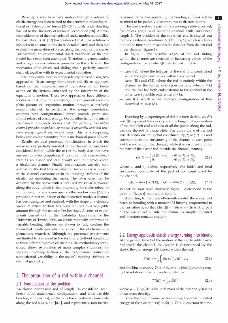
of the channel (figure 1).

In figure 1, the possible stages of the rod sliding

within the channel are sketched at increasing values of the

configurational parameter j(t), as defined in table 1:

— case (A), where the left part of the rod is unconstrained

while the right end moves within the channel;

— cases (B1) and (B2), where the rod is entirely within the

channel in the former case (possible only when l , L)

and the rod has both ends external to the channel in the

latter case (possible only when l . L);

— case (C), which is the opposite configuration of that

described in case (A).

Denoting by a superimposed dot the time derivative, _j(t)and €j(t) represent the velocity and the tangential acceleration

of the rod’s left end and also of all the points along the rod,

because the rod is inextensible. The curvature k of the rod

axis depends on the global coordinate s(s, t) ¼ j(t) þ s and

corresponds to the curvature x of the channel at each point

s of the rod within the channel, while it is assumed null for

the part of the elastic rod outside the channel, namely

kðs, tÞ ¼ xðjðtÞ þ sÞ, s [ ½s1ðtÞ, s2ðtÞ�,0, s � ½s1ðtÞ, s2ðtÞ�,

�ð2:1Þ

where s1 and s2 define, respectively, the initial and final

curvilinear coordinate of the part of rod constrained by

the channel,

s1(t) ¼ max {�j(t), 0}, s2(t) ¼ min {l, L� j(t)}, ð2:2Þ

so that the four cases shown in figure 1 correspond to the

pairs fs1(t), s2(t)g reported in table 1.

According to the Euler–Bernoulli model, the elastic rod

reacts to bending with a moment M linearly proportional to

the curvature k, so that M(s, j(t)) ¼ B(s)k(s þ j(t)). Any part

of the elastic rod outside the channel is simply unloaded

and therefore remains straight.

2.2. Energy approach: elastic energy turning into kineticAt the generic time t of the motion of the inextensible elastic

rod inside the channel, the system is characterized by the

elastic flexural energy E(t) stored within the rod,

E(j(t)) ¼ 1

2

ðl

0

B(s)k2(s, j(t)) ds, ð2:3Þ

and the kinetic energy T (t) of the rod, which (assuming neg-

ligible rotational inertia) can be written as

T ( _j(t)) ¼ 1

2m[ _j(t)]2, ð2:4Þ

where m ¼Ð l

0 g(s) ds is the total mass of the rod and g(s) is its

linear mass density.

Since the rigid channel is frictionless, the total potential

energy of the system,3 V(t) ¼ E(t)þ T (t), is constant in time,

lx(t)

s

LL

(B2) l > L

(B1) l < L(A)

(C)

x(t) Œ (–l, min{0, L – l})

x(t) Π(max{0, L Рl}, L)x(t) Π(L Рl, 0)

x(t) Π(0, L Рl)s

Figure 1. An inextensible elastic rod (rectilinear in its undeformed configuration) of length l is moving within a frictionless and smooth curvilinear channel. Itsconfiguration is defined through the evolution in time of the curvilinear coordinate j(t), which singles out the position of the left end. Four cases arise: (A) and (C)where one of the rod’s ends is inside the channel while the other remains unrestrained; (B1) where the whole rod is inside the channel and (B2) where the rodoccupies the whole channel. (Online version in colour.)

Table 1. Ranges of the configurational parameter j and values of the coordinates s1 and s2, together with their respective derivatives, for the four cases.

case A B1 B2 C

j(t) [ (� l, min {0, L� l}) [ (0, L 2 l ) [ (L 2 l, 0) [ (max {0, L� l}, L)

s1(t) 2j(t) 0 2j(t) 0

s2(t) l l L 2 j(t) L 2 j(t)

1þ @s1(t)@j(t)

0 1 0 1

11þ @s2(t)@j(t)

1 1 0 0

rsif.royalsocietypublishing.orgJ.R.Soc.Interface

14:20170055

3

on May 31, 2017http://rsif.royalsocietypublishing.org/Downloaded from

so that its time derivative vanishes

_E(t)þ _T (t) ¼ 0, ð2:5Þ

which leads to

@E(j)

@jþ m €j

� �_j(t) ¼ 0: ð2:6Þ

Defining the propulsive force P(t) as

P(t) ¼ � @E(j(t))@j(t)

, ð2:7Þ

the equation of the longitudinal motion of the rod within the

channel follows in the form

m €j(t) ¼ P(t): ð2:8Þ

Note from equation (2.7) that the propulsive force P is a

‘resultant configurational force’, which is different from

zero only when a change in the elastic strain energy E of

the rod occurs through a change in the configurational

parameter j, a situation similar to the Eshelby-like forces in

elastic systems constrained by a sliding sleeve [26].

The two types of jump discontinuity are now introduced

within the part of the rod constrained by the channel. One

discontinuity is in the bending stiffness B(s) of the elastic

rod at the local coordinate s ¼ l1 [ (s1, s2)

½½B(l1)�� ¼ B(lþ1 )� B(l�1 ), ð2:9Þ

and the other discontinuity is in the curvature of the channel

at the global coordinate s ¼ L1 [ ( j þ s1, j þ s2)

½½x(L1)�� ¼ x(Lþ1 )� x(L�1 ), ð2:10Þ

where the dependence on time has been omitted for simpli-

city (and also in the following). It is noted that the

superscripts þ and 2 define, respectively, the one-sided

limit of the relevant quantity from the negative or positive

direction.

Considering that the elastic energy (2.3) can be rewritten

as

E(j) ¼ 1

2

ðs2(j)

s1(j)

B(s)x2(jþ s) ds, ð2:11Þ

which is an integral with moving limits s1(j) and s2(j), and

that the derivatives of the curvature field x(j þ s) with respect

to j and s are identical,

@x(jþ s)

@j¼ @x(jþ s)

@s, ð2:12Þ

the propulsive force (2.7) can be calculated by means of the

Leibniz integral rule as

P ¼ @s1ðjÞ@j

Bðs1ðjÞÞx2ðjþ s1ðjÞÞ2

� @s2ðjÞ@j

Bðs2ðjÞÞx2ðjþ s2ðjÞÞ2

� BðL1 � jÞ½½x2ðL1Þ��2

�ðL�1 �j

s1ðjÞBðsÞxðjþ sÞx0ðjþ sÞds

�ðs2ðjÞ

Lþ1�j

BðsÞxðjþ sÞx0ðjþ sÞds; ð2:13Þ

rsif.royalsocietypublishing.orgJ.R.Soc.Interface

14:20170055

4

on May 31, 2017http://rsif.royalsocietypublishing.org/Downloaded from

or, equivalently, after integration by parts, as

P ¼ 1þ @s1ðjÞ@j

� �Bðs1ðjÞÞx2ðjþ s1ðjÞÞ

2

� 1þ @s2ðjÞ@j

� �Bðs2ðjÞÞx2ðjþ s2ðjÞÞ

2

þ ½½Bðl1Þ��x2ðjþ l1Þ

2þ 1

2

ðl�1

s1ðjÞB0ðsÞx2ðjþ sÞds

þ 1

2

ðs2ðjÞ

lþ1

B0ðsÞx2ðjþ sÞds: ð2:14Þ

Equations (2.13) and (2.14) are fully equivalent and provide the

same value of the propulsive force P for the given geometry and

stiffness properties. However, the two formulae are expressed in

a way that only one type of discontinuity appears. Indeed, the

former (the latter) expression highlights the influence of only

jump discontinuities in the squared channel curvature ½½x2�� (in

the bending stiffness ½½B��), while the discontinuity in the stiffness

(in the channel curvature) does not explicitly appear.

Specifying equation (2.14) for the four cases shown in figure

1, and considering the values of the derivatives @sj(j)/@j ( j ¼ 1,

2) as computed in table 1, the propulsive force P simplifies to

— case A

P ¼ �Bð�jÞx2ð0Þ2

� BðL1 � jÞ½½x2ðL1Þ��2

�ðL�1 �j

�jBðsÞxðjþ sÞx 0ðjþ sÞds

�ðl

Lþ1�j

BðsÞxðjþ sÞx 0ðjþ sÞds, ð2:15Þ

or, equivalently,

P ¼ �BðlÞx2ðjþ lÞ2

þ ½½Bðl1Þ��x2ðjþ l1Þ2

þ 1

2

ðl�1

�jB0ðsÞx2ðjþ sÞdsþ 1

2

ðl

lþ1

B0ðsÞx2ðjþ sÞds;

ð2:16Þ

— case B1

P ¼ �BðL1 � jÞ½½x2ðL1Þ��2

�ðL�1 �j

0

BðsÞxðjþ sÞx0ðjþ sÞds

�ðl

Lþ1�j

BðsÞxðjþ sÞx0ðjþ sÞds, ð2:17Þ

or, equivalently,

P ¼ Bð0Þx2ðjÞ2

� BðlÞx2ðjþ lÞ2

þ ½½Bðl1Þ��x2ðjþ l1Þ2

þ 1

2

ðl�1

0

B0ðsÞx2ðjþ sÞdsþ 1

2

ðl

lþ1

B0ðsÞx2ðjþ sÞds;

ð2:18Þ

— case B2

P ¼ BðL� jÞx2ðLÞ2

� Bð�jÞx2ð0Þ2

� BðL1 � jÞ½½x2ðL1Þ��2

�ðL�1 �j

�jBðsÞxðjþ sÞx 0ðjþ sÞds

�ðL�j

Lþ1�j

BðsÞxðjþ sÞx0ðjþ sÞds, ð2:19Þ

or, equivalently,

P ¼ ½½Bðl1Þ��x2ðjþ l1Þ2

þ 1

2

ðl�1

�jB0ðsÞx2ðjþ sÞds

þ 1

2

ðL�j

lþ1

B0ðsÞx2ðjþ sÞds; ð2:20Þ

— case C

P ¼ BðL� jÞx2ðLÞ2

� BðL1 � jÞ½½x2ðL1Þ��2

�ðL�1 �j

0

BðsÞxðjþ sÞx 0ðjþ sÞds

�ðL�j

Lþ1�j

BðsÞxðjþ sÞx0ðjþ sÞds, ð2:21Þ

or, equivalently,

P ¼ Bð0Þx2ðjÞ2

þ ½½Bðl1Þ��x2ðjþ l1Þ2

þ 1

2

ðl�1

0

B0ðsÞx2ðjþ sÞdsþ 1

2

ðL�j

lþ1

B0ðsÞx2ðjþ sÞds:

ð2:22Þ

Equations (2.15)–(2.22) provide the theoretical evaluation

of the propulsive force P that may be analytically or numeri-

cally computed for given distributions of bending stiffness

B(s) along the rod and curvature of the channel x(s). It is

worth mentioning that only the case B1 was previously

analysed in [12] under several restrictive hypotheses (continu-

ous channel curvature and rod bending stiffness, null bending

moment and axial force at the end of the rod) so that equation

(2.18) reduces to the result presented in [12] when ½½B(l1)�� ¼ 0.

Note that equations (2.7) and (2.10) of [12] have incorrect signs.

In addition, the normal forces internal to the snake have been

erroneously disregarded in equation (2.7) of [30].

2.3. Propulsion from Newton’s second lawand micromechanics

Equations (2.13) and (2.14) provide the propulsive force in a

global sense. This force is the result of the channel tangential

reactions against the rod (which could be thought to be null

at a first—mistaken—glance because the channel is friction-

less), the knowledge of which is fundamental in the

determination of the stress state in the snake’s body during

motion. These reactions, which have until now only been

used to analyse the special case of the concentrated force at

the end of the rod within a channel [5], can be derived with

consideration of the dynamics of the rod’s element and of

the micromechanics of the elastic rod at its ends, at the

entrance or the exit of the channel and at discontinuity

points in the channel curvature or the rod’s bending stiffness.

The equilibrium equations for an elementary portion of a

planar rod in a curved configuration (figure 2), defined by the

curvature k(s), can be written in the non-inertial frame of

reference attached to the rod (at its left end, the origin of

the curvilinear coordinate s) as

T0(s)�N(s)k(s)þ fr(s) ¼ 0,

M0(s)� T(s)þ fu(s) ¼ 0

and N0(s)þ T(s)k(s)þ fs(s) ¼ 0,

9>=>; ð2:23Þ

where T(s), N(s) and M(s) are the shear and axial forces, and

the bending moment, respectively, while fr(s), fs(s) and fu(s)

N + dN

M + dM

T + dT

fqdsfrds

fsds

M

TN

Figure 2. Free body diagram of an element of the elastic rod in thedeformed configuration, where M(s), T(s) and N(s) denote bendingmoment, shear and axial forces, respectively, while fr(s), fs(s) and fu(s) arethe distributed external forces (as the sum of the real and apparentforces) applied to the rod, respectively, in the transverse, axial and rotationaldirections. (Online version in colour.)

rsif.royalsocietypublishing.orgJ.R.Soc.Interface

14:20170055

5

on May 31, 2017http://rsif.royalsocietypublishing.org/Downloaded from

are the distributed (total) forces applied to the rod, respect-

ively, in the transverse, axial and rotational directions. By

means of D’Alembert’s principle, the equations of motion

for an elementary portion of the rod can be obtained from

equation (2.23) by considering the distributed forces fr(s),

fs(s) and fu(s) to be the sum of the real distributed forces (pro-

vided by the contact with the channel) and the apparent

distributed forces (given by the negative of the inertia

forces per unit length). More specifically

— for the part of the rod constrained by the channel, k(s) ¼

x(s), and neglecting the rotational inertia of the rod, the

distributed forces are given by

frðsÞ ¼ pðsÞ � gðsÞ _j2xðsÞ,

fuðsÞ ¼ mðsÞ,

fsðsÞ ¼ qðsÞ � gðsÞ€j,

9>>=>>;

s [ ðs1, s2Þ, ð2:24Þ

where p(s), q(s) and m(s) represent the channel reactions

applied to the rod, respectively, in the transverse, axial

and rotational directions;

— for the part of the rod outside the channel, this is assumed

to remain straight (flexural vibrations are disregarded),

k(s) ¼ 0, so that the distributed forces are given by

frðsÞ ¼ 0,

fuðsÞ ¼ 0,

fsðsÞ ¼ �gðsÞ €j,

9>>=>>;

s [ ½0,s1ðtÞ�< ½s2ðtÞ, l�: ð2:25Þ

In this case, considering null boundary conditions at the

ends, the integration of the equations of motion leads to

MðsÞ ¼ 0,

TðsÞ ¼ 0,

N0ðsÞ ¼ gðsÞ €j,

9>>=>>;

s [ ½0, s1ðtÞ�< ½s2ðtÞ, l�: ð2:26Þ

It is worth remarking that, in the case of quasi-static

motion (namely, negligible inertial density forces), the

distributed forces fr(s), fu(s), fs(s) would all be either null or

coincident with the channel reactions p(s), m(s), q(s),

respectively, for the parts of the rod outside and within the

channel.

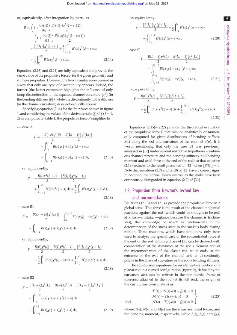
2.3.1. Micromechanics of a rod inside the channelThe tangential reactions acting at the rod’s ends, at the chan-

nel entrance/exit, at the points of discontinuity of the channel

curvature or of the rod’s bending stiffness are derived here.

These counter-intuitive reactions are strictly related to the

deformability of the constrained rod and to the non-

rectilinearity of the channel and have been found in other

‘non-classical’ situations [26,28,31].

Relaxing for a moment the assumption that the rod is per-

fectly tight to the channel, a clearance is introduced in the

channel constraining the elastic rod as shown in figure 3.

Owing to the presence of the gap, assumed small, between

the elastic rod and the channel, the former always has a zone

of detachment (singled out by the angle F and having

arc-length a) from the latter. In the micromechanical analysis

developed below it is shown that in the limit when the gap

vanishes, so that the detachment region vanishes too, a non-

null tangential reaction is developed by the frictionless channel.

In figure 3, three possible cases of interest are sketched,

namely: (i) the rod’s end is inside the channel; (ii) the channel

curvature has a discontinuity; and (iii) the rod’s end is outside

the channel. In all cases, the reaction force F is orthogonal to

the channel, which is frictionless. Below, these three cases

will be analysed together with the further case in which (iv)

the rod has a discontinuity in the bending stiffness.

Tangential reaction at the rod end inside the channelThe situation when one end of the elastic rod is inside the

frictionless channel with radius of curvature 1/x is sketched

in figure 3a.

It is evident that the rod end is subject to the channel reac-

tion F only, orthogonal to the upper contour of the channel.

This force provides the moment M ¼ FF/x at the point (at

the distance a ¼ F/x from the rod’s end) where the elastic

rod becomes adherent to the profile, so that M ¼ Bx. At

that point the internal axial action can be approximated as

F sinF � FF, which becomes B x2, the resultant axial force

developing at the rod’s end within a channel.

With reference to the curvilinear coordinate system s, if

the left and the right ends of the rod are inside the channel,

s1 ¼ 0 and s2 ¼ l, the compressive reaction forces are

realized by the channel at the edges of the rod

N(0þ) ¼ �B(0)x2(j), cases B1 and C, and

N(l�) ¼ �B(l)x2(jþ l), cases A and B, ð2:27Þ

which have also been obtained using the principle of virtual

power in [5] and are similar to the tangential reaction devel-

oping in a perfectly frictionless curvilinear profile

constraining a clamped end of the rod [31].

Tangential reaction at a discontinuity point in the channelcurvatureIn the case when there is a jump in the curvature along the

channel (figure 3b), the curvature of the rod takes a value

different from the channel curvature because a small gap is

present. In particular, the rod has a transition length along

which its curvature passes from the channel curvature

before to that after the jump. With reference to figure 3b,

two concentrated contact reactions F2 and Fþ develop

orthogonal to the upper and lower contours of the channel

at the rod’s two detachment points. Owing to a difference

in the angle F in the direction of the two reactions, a tangen-

tial resultant is expected. At equilibrium, in the limit of

vanishing detachment length a, the two reactions orthogonal

to the channel tend to the same value, Fþ ¼ F2 ¼ F, and the

tangential resultant is given by F sinF � FF. The bending

moments at the two detachment points are defined by the rel-

evant curvature imposed by the channel, so that they are

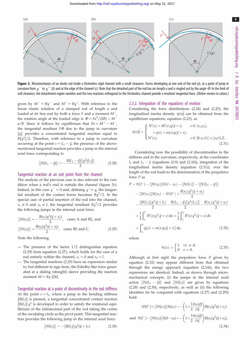
F –

F +M –

F –

M

F

F M F +

1/ |c |

1/ |c |1/ |c –|

1/ |c+ |

F FF

M +

(a) (b) (c)

Figure 3. Micromechanics of an elastic rod inside a frictionless rigid channel with a small clearance. Forces developing at one end of the rod (a), at a point of jump incurvature from x2 to xþ (b) and at the edge of the channel (c). Note that the detached part of the rod has arc-length a and is singled out by the angle F. In the limit ofnull clearance, the detachment region vanishes and the two reactions orthogonal to the frictionless channel provide a resultant tangential force. (Online version in colour.)

rsif.royalsocietypublishing.orgJ.R.Soc.Interface

14:20170055

6

on May 31, 2017http://rsif.royalsocietypublishing.org/Downloaded from

given by M2 ¼ Bx2 and Mþ ¼ Bxþ. With reference to the

linear elastic solution of a clamped rod of length a and

loaded at its free end by both a force F and a moment M2,

the rotation angle at the loaded edge is F ¼ Fa2/(2B) þM2

a/B. Since it follows by equilibrium that Fa ¼Mþ2 M2,

the tangential resultant FF due to the jump in curvature

½½x�� provides a concentrated tangential reaction equal to

B½½x2��=2. Therefore, with reference to a jump in curvature

occurring at the point s ¼ L1 2 j, the presence of the above-

mentioned tangential reaction provides a jump in the internal

axial force corresponding to

½½N(L1 � j)�� ¼ �B(L1 � j)½½x2(L1)��2

: ð2:28Þ

Tangential reaction at an exit point from the channelThe analysis of the previous case is also relevant to the con-

dition when a rod’s end is outside the channel (figure 3c).

Indeed, in this case x2 ¼ 0 and, defining xþ¼ x, the tangen-

tial resultant of the contact forces becomes Bx2/2. In the

special case of partial insertion of the rod into the channel,

s1 = 0 and s2 = l, the tangential resultant Bx2/2 provides

the following jumps in the internal axial force:

½½N(s1)�� ¼ �B(s1)x2(jþ s1)

2, cases A and B2, and

½½N(s2)�� ¼ B(s2)x2(jþ s2)

2, cases B2 and C: ð2:29Þ

Note the following.

— The presence of the factor 1/2 distinguishes equation

(2.29) from equation (2.27), which holds for the case of a

rod entirely within the channel, s1 ¼ 0 and s2 ¼ l.— The tangential reactions (2.29) have an expression similar

to, but different in sign from, the Eshelby-like force gener-

ated at a sliding (straight) sleeve providing the reaction

moment M ¼ Bx [26].

Tangential reaction at a point of discontinuity in the rod stiffnessAt the point s ¼ l1, where a jump in the bending stiffness

½½B(l1)�� is present, a tangential concentrated contact reaction

½½B(l1)��x2 is developed in order to satisfy the rotational equi-

librium of the infinitesimal part of the rod taking the centre

of the osculating circle as the pivot point. This tangential reac-

tion provides the following jump in the internal axial force:

½½N(l1)�� ¼ �½½B(l1)��x2(jþ l1): ð2:30Þ

2.3.2. Integration of the equations of motion

Considering the force distributions (2.24) and (2.25), the

longitudinal inertia density g(s) €j can be obtained from the

equilibrium equations, equation (2.23), as

gðsÞ€j ¼N0ðsÞ þM0ðsÞxðjþ sÞ

þ qðsÞ þmðsÞxðjþ sÞ,

s [ ðs1,s2Þ,

N0ðsÞ, s [ ½0, s1ðtÞ�< ½s2ðtÞ,l�:

8><>:

ð2:31Þ

Considering now the possibility of discontinuities in the

stiffness and in the curvature, respectively, at the coordinates

l1 and L1 2 j (equations (2.9) and (2.10)), integration of the

longitudinal inertia density (equation (2.31)), over the

length of the rod leads to the determination of the propulsive

force P as

P ¼ Nðl�Þ � ½½Nðs2Þ��Hðl� s2Þ � ½½Nðl1Þ�� � ½½NðL1 � jÞ��

� ½½Nðs1Þ��Hðs1Þ �Nð0þÞ þ Bðs2Þx2ðjþ s2Þ2

� ½½Bðl1Þ��x2ðjþ l1Þ

2� BðL1 � jÞ½½x2ðL1Þ��

2� Bðs1Þx2ðjþ s1Þ

2

þ 1

2

ðl�1

s1

B0ðsÞx2ðjþ sÞdsþ 1

2

ðs2

lþ1

B0ðsÞx2ðjþ sÞds

þðs2

s1

½qðsÞ þmðsÞxðjþ sÞ�ds, ð2:32Þ

where

HðxÞ ¼ 1 8x = 0,0 x ¼ 0:

�ð2:33Þ

Although at first sight the propulsive force P given by

equation (2.32) may appear different from that obtained

through the energy approach (equation (2.14)), the two

expressions are identical. Indeed, as shown through micro-

mechanical concepts, (i) the jumps in the internal axial

action ½½N(L1 � j)�� and ½½N(l1)�� are given by equations

(2.28) and (2.30), respectively, as well as (ii) the following

identities (to be compared with equations (2.27) and (2.29))

hold:

N(0þ)þ½½N(s1)��H(s1)¼� 1þ1

2

@s1(j)

@j

� �B(s1)x2(jþs1)

and N(l�)�½½N(s2)��H(l�s2)¼� 1þ1

2

@s2(j)

@j

� �B(s2)x2(jþs2),

ð2:34Þ

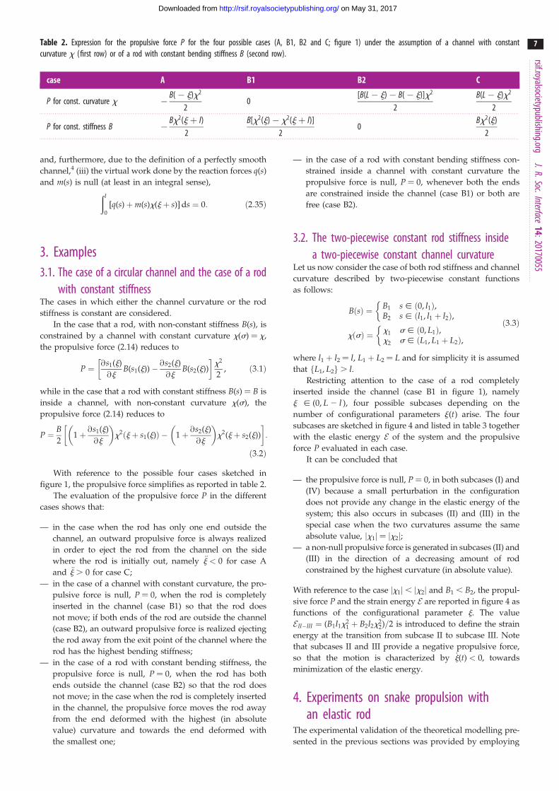
Table 2. Expression for the propulsive force P for the four possible cases (A, B1, B2 and C; figure 1) under the assumption of a channel with constantcurvature x (first row) or of a rod with constant bending stiffness B (second row).

case A B1 B2 C

P for const. curvature x � B(� j)x2

20

[B(L� j)� B(� j)]x2

2B(L� j)x2

2

P for const. stiffness B � Bx2(jþ l)2

B[x2(j)� x2(jþ l)]2

0Bx2(j)

2

rsif.royalsocietypublishing.orgJ.R.Soc.Interface

7

on May 31, 2017http://rsif.royalsocietypublishing.org/Downloaded from

and, furthermore, due to the definition of a perfectly smooth

channel,4 (iii) the virtual work done by the reaction forces q(s)

and m(s) is null (at least in an integral sense),

ðl

0

[q(s)þm(s)x(jþ s)] ds ¼ 0: ð2:35Þ

14:20170055

3. Examples3.1. The case of a circular channel and the case of a rod

with constant stiffnessThe cases in which either the channel curvature or the rod

stiffness is constant are considered.

In the case that a rod, with non-constant stiffness B(s), is

constrained by a channel with constant curvature x(s) ¼ x,

the propulsive force (2.14) reduces to

P ¼ @s1(j)

@jB(s1(j))� @s2(j)

@jB(s2(j))

� �x2

2, ð3:1Þ

while in the case that a rod with constant stiffness B(s) ¼ B is

inside a channel, with non-constant curvature x(s), the

propulsive force (2.14) reduces to

P ¼ B2

1þ @s1(j)

@j

� �x2 jþ s1(j)ð Þ � 1þ @s2(j)

@j

� �x2(jþ s2(j))

� �:

ð3:2Þ

With reference to the possible four cases sketched in

figure 1, the propulsive force simplifies as reported in table 2.

The evaluation of the propulsive force P in the different

cases shows that:

— in the case when the rod has only one end outside the

channel, an outward propulsive force is always realized

in order to eject the rod from the channel on the side

where the rod is initially out, namely €j < 0 for case A

and €j . 0 for case C;

— in the case of a channel with constant curvature, the pro-

pulsive force is null, P ¼ 0, when the rod is completely

inserted in the channel (case B1) so that the rod does

not move; if both ends of the rod are outside the channel

(case B2), an outward propulsive force is realized ejecting

the rod away from the exit point of the channel where the

rod has the highest bending stiffness;

— in the case of a rod with constant bending stiffness, the

propulsive force is null, P ¼ 0, when the rod has both

ends outside the channel (case B2) so that the rod does

not move; in the case when the rod is completely inserted

in the channel, the propulsive force moves the rod away

from the end deformed with the highest (in absolute

value) curvature and towards the end deformed with

the smallest one;

— in the case of a rod with constant bending stiffness con-

strained inside a channel with constant curvature the

propulsive force is null, P ¼ 0, whenever both the ends

are constrained inside the channel (case B1) or both are

free (case B2).

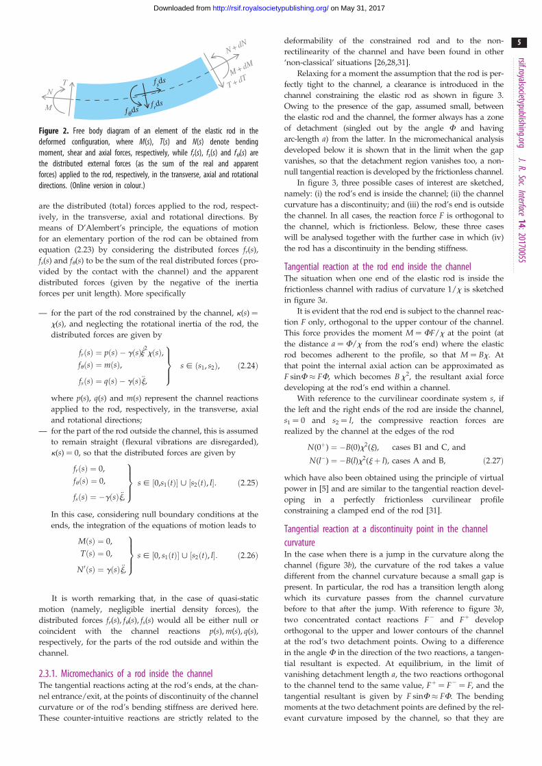
3.2. The two-piecewise constant rod stiffness insidea two-piecewise constant channel curvature

Let us now consider the case of both rod stiffness and channel

curvature described by two-piecewise constant functions

as follows:

BðsÞ ¼ B1 s [ ð0, l1Þ,B2 s [ ðl1, l1 þ l2Þ,

�

xðsÞ ¼ x1 s [ ð0, L1Þ,x2 s [ ðL1, L1 þ L2Þ,

� ð3:3Þ

where l1 þ l2 ¼ l, L1 þ L2 ¼ L and for simplicity it is assumed

that fL1, L2g. l.Restricting attention to the case of a rod completely

inserted inside the channel (case B1 in figure 1), namely

j [ (0, L 2 l ), four possible subcases depending on the

number of configurational parameters j(t) arise. The four

subcases are sketched in figure 4 and listed in table 3 together

with the elastic energy E of the system and the propulsive

force P evaluated in each case.

It can be concluded that

— the propulsive force is null, P ¼ 0, in both subcases (I) and

(IV) because a small perturbation in the configuration

does not provide any change in the elastic energy of the

system; this also occurs in subcases (II) and (III) in the

special case when the two curvatures assume the same

absolute value, jx1j ¼ jx2j;— a non-null propulsive force is generated in subcases (II) and

(III) in the direction of a decreasing amount of rod

constrained by the highest curvature (in absolute value).

With reference to the case jx1j , jx2j and B1 , B2, the propul-

sive force P and the strain energy E are reported in figure 4 as

functions of the configurational parameter j. The value

EII�III ¼ (B1l1x21 þ B2l2x2

2)=2 is introduced to define the strain

energy at the transition from subcase II to subcase III. Note

that subcases II and III provide a negative propulsive force,

so that the motion is characterized by _j(t) < 0, towards

minimization of the elastic energy.

4. Experiments on snake propulsion withan elastic rod

The experimental validation of the theoretical modelling pre-

sented in the previous sections was provided by employing

L1 – l L1 – l1 L – lL1

PII

PIII

E, P

(IV)

(III)

(II)

L1

l1 l 2

(I)

0

1/ |c 2|

1/ |c 1|x(t)

x

EIVEII–III

EI

Figure 4. With reference to case B1 (figure 1), four subcases (I, II, III and IV) are depicted for a rod of piecewise constant bending stiffness constrained inside achannel of piecewise constant curvature, at increasing curvilinear coordinate j(t) defined as in table 3. The elastic energy E (green) and the propulsive force P (red)are plotted as functions of the curvilinear coordinate j. The plot is representative of the case jx1j , jx2j and B1 , B2. (Online version in colour.)

rsif.royalsocietypublishing.orgJ.R.Soc.Interface

14:20170055

8

on May 31, 2017http://rsif.royalsocietypublishing.org/Downloaded from

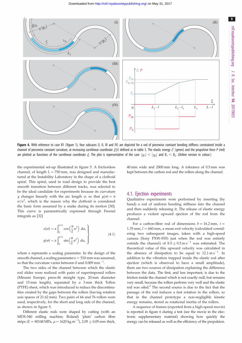
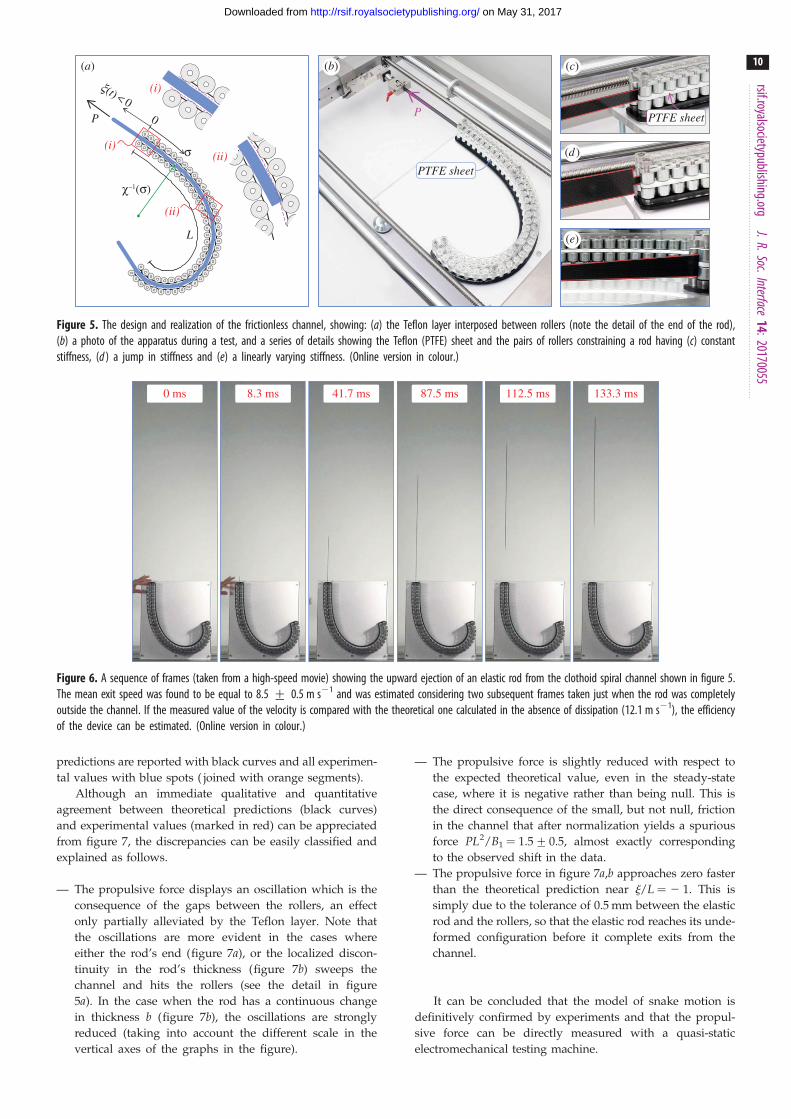
the experimental set-up illustrated in figure 5. A frictionless

channel, of length L ¼ 750 mm, was designed and manufac-

tured at the Instability Laboratory in the shape of a clothoid

spiral. This spiral, used in road design to provide the best

smooth transition between different tracks, was selected to

be the ideal candidate for experiments because its curvature

x changes linearly with the arc length s, so that x(s) ¼ p

s/a2, which is the reason why the clothoid is considered

the basic form assumed by a snake during its motion [30].

This curve is parametrically expressed through Fresnel

integrals as [32]

x(s) ¼ aðs=a

0

cosp

2u2

� �du,

y(s) ¼ aðs=a

0

sinp

2u2

� �du,

9>>>=>>>;

ð4:1Þ

where a represents a scaling parameter. In the design of the

smooth channel, a scaling parameter a ¼ 510 mm was assumed,

so that the curvature varies between 0 and 0.009 mm21.

The two sides of the channel between which the elastic

rod slides were realized with pairs of superimposed rollers

(Misumi Europe; press-fit straight type, 20 mm diameter

and 15 mm length), separated by a 3 mm thick Teflon

(PTFE) sheet, which was introduced to reduce the discontinu-

ities created by the gaps between the rollers (having rotation

axis spaces of 21.62 mm). Two pairs of 66 and 76 rollers were

used, respectively, for the short and long side of the channel,

as shown in figure 5.

Different elastic rods were shaped by cutting (with an

MDX-540 milling machine; Roland) ‘plain’ carbon fibre

strips (E¼ 80148 MPa, r¼ 1620 kg m23), 2.05+0.05 mm thick,

40 mm wide and 2000 mm long. A tolerance of 0.5 mm was

kept between the carbon rod and the rollers along the channel.

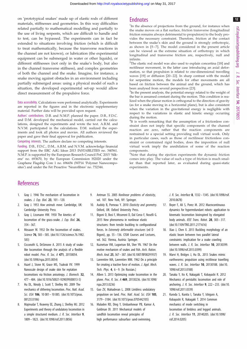
4.1. Ejection experimentsQualitative experiments were performed by inserting (by

hand) a rod of uniform bending stiffness into the channel

and then suddenly releasing it. The release of elastic energy

produces a violent upward ejection of the rod from the

channel.

For a carbon-fibre rod of dimensions b ¼ 16.2 mm, t ¼1.35 mm, l ¼ 660 mm, a mean exit velocity (calculated consid-

ering two subsequent images, taken with a high-speed

camera (Sony PXW-FS5) just when the rod was entirely

outside the channel) of 8.5+0.5 m s21 was estimated. The

theoretical value of this upward velocity was calculated in

the absence of dissipation to be equal to 12.1 m s21. In

addition to the vibration trapped inside the elastic rod after

ejection (which is observed to have a small amplitude),

there are two sources of dissipation explaining the difference

between the data. The first, and less important, is due to the

friction inside the channel which is not exactly null, but remains

very small, because the rollers perform very well and the elastic

rod was oiled.5 The second source is due to the fact that the

passage of the rod induces a fast rotation in the rollers, so

that in the channel prototype a non-negligible kinetic

energy remains, stored as rotational inertia of the rollers.

A sequence of frames (exported from a high-speed movie)

is reported in figure 6 during a test (see the movie in the elec-

tronic supplementary material) showing how quickly the

energy can be released as well as the efficiency of the propulsion.

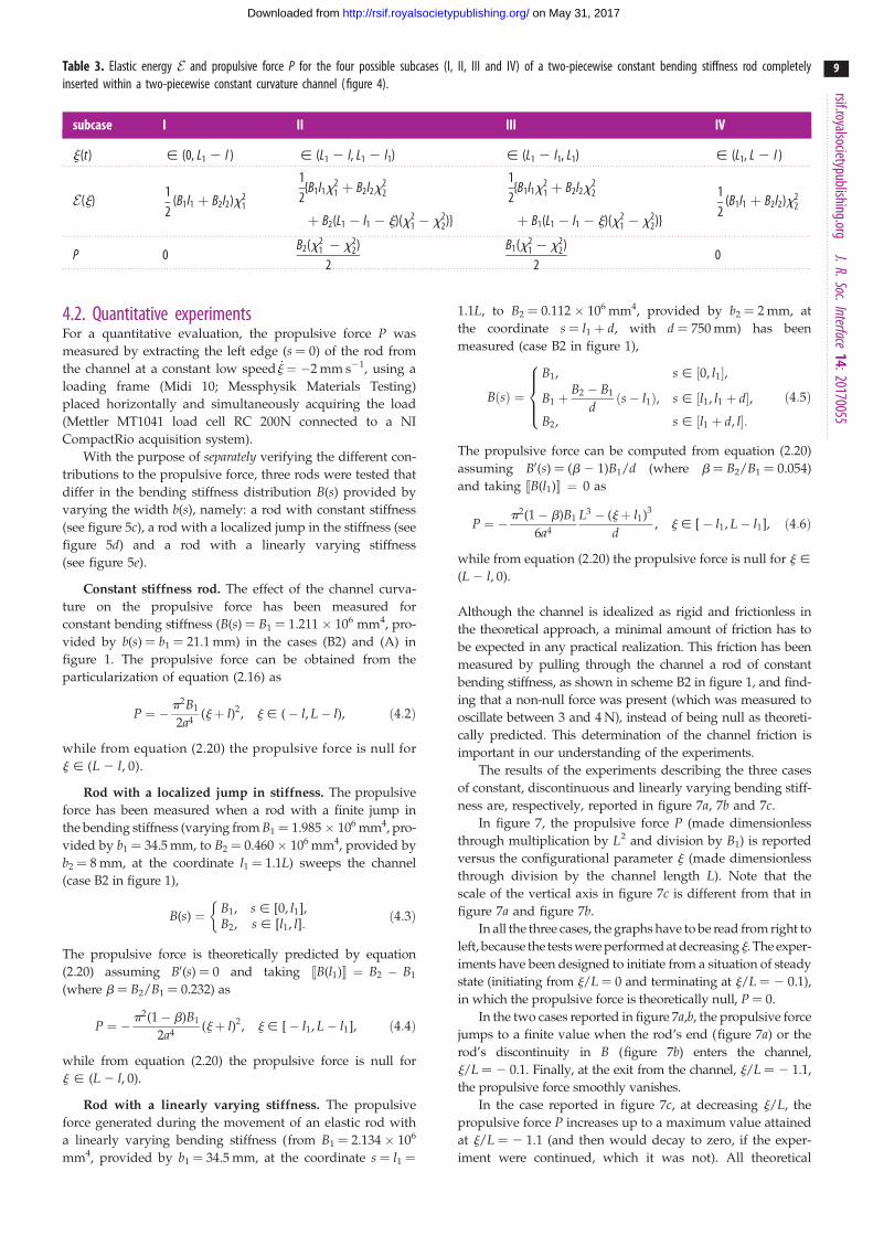
Table 3. Elastic energy E and propulsive force P for the four possible subcases (I, II, III and IV) of a two-piecewise constant bending stiffness rod completelyinserted within a two-piecewise constant curvature channel (figure 4).

subcase I II III IV

j(t) [ (0, L1 2 l ) [ (L1 2 l, L1 2 l1) [ (L1 2 l1, L1) [ (L1, L 2 l )

E(j)12

(B1 l1 þ B2l2)x21

12

{B1l1x21 þ B2 l2x

22

þ B2(L1 � l1 � j)(x21 � x2

2)}

12

{B1l1x21 þ B2l2x

22

þ B1(L1 � l1 � j)(x21 � x2

2)}

12

(B1l1 þ B2l2)x22

P 0B2(x2

1 � x22)

2B1(x2

1 � x22)

20

rsif.royalsocietypublishing.orgJ.R.Soc.Interface

14:20170055

9

on May 31, 2017http://rsif.royalsocietypublishing.org/Downloaded from

4.2. Quantitative experimentsFor a quantitative evaluation, the propulsive force P was

measured by extracting the left edge (s ¼ 0) of the rod from

the channel at a constant low speed _j ¼ �2 mm s21, using a

loading frame (Midi 10; Messphysik Materials Testing)

placed horizontally and simultaneously acquiring the load

(Mettler MT1041 load cell RC 200N connected to a NI

CompactRio acquisition system).

With the purpose of separately verifying the different con-

tributions to the propulsive force, three rods were tested that

differ in the bending stiffness distribution B(s) provided by

varying the width b(s), namely: a rod with constant stiffness

(see figure 5c), a rod with a localized jump in the stiffness (see

figure 5d) and a rod with a linearly varying stiffness

(see figure 5e).

Constant stiffness rod. The effect of the channel curva-

ture on the propulsive force has been measured for

constant bending stiffness (B(s) ¼ B1 ¼ 1.211 � 106 mm4, pro-

vided by b(s) ¼ b1 ¼ 21.1 mm) in the cases (B2) and (A) in

figure 1. The propulsive force can be obtained from the

particularization of equation (2.16) as

P ¼ �p2B1

2a4(jþ l)2, j [ (� l, L� l), ð4:2Þ

while from equation (2.20) the propulsive force is null for

j [ (L 2 l, 0).

Rod with a localized jump in stiffness. The propulsive

force has been measured when a rod with a finite jump in

the bending stiffness (varying from B1 ¼ 1.985 � 106 mm4, pro-

vided by b1 ¼ 34.5 mm, to B2 ¼ 0.460 � 106 mm4, provided by

b2 ¼ 8 mm, at the coordinate l1 ¼ 1.1L) sweeps the channel

(case B2 in figure 1),

B(s) ¼ B1, s [ [0, l1],B2, s [ [l1, l]:

�ð4:3Þ

The propulsive force is theoretically predicted by equation

(2.20) assuming B0(s) ¼ 0 and taking ½½B(l1)�� ¼ B2 � B1

(where b ¼ B2/B1 ¼ 0.232) as

P ¼ �p2(1� b)B1

2a4(jþ l)2, j [ [� l1, L� l1], ð4:4Þ

while from equation (2.20) the propulsive force is null for

j [ (L 2 l, 0).

Rod with a linearly varying stiffness. The propulsive

force generated during the movement of an elastic rod with

a linearly varying bending stiffness (from B1 ¼ 2.134 � 106

mm4, provided by b1 ¼ 34.5 mm, at the coordinate s ¼ l1 ¼

1.1L, to B2 ¼ 0.112 � 106 mm4, provided by b2 ¼ 2 mm, at

the coordinate s ¼ l1 þ d, with d ¼ 750 mm) has been

measured (case B2 in figure 1),

BðsÞ ¼

B1, s [ ½0, l1�,

B1 þB2 � B1

dðs� l1Þ, s [ ½l1, l1 þ d�,

B2, s [ ½l1 þ d, l�:

8>><>>:

ð4:5Þ

The propulsive force can be computed from equation (2.20)

assuming B0(s) ¼ (b 2 1)B1/d (where b ¼ B2/B1 ¼ 0.054)

and taking ½½B(l1)�� ¼ 0 as

P ¼ �p2(1� b)B1

6a4

L3 � (jþ l1)3

d, j [ [� l1, L� l1], ð4:6Þ

while from equation (2.20) the propulsive force is null for j [

(L 2 l, 0).

Although the channel is idealized as rigid and frictionless in

the theoretical approach, a minimal amount of friction has to

be expected in any practical realization. This friction has been

measured by pulling through the channel a rod of constant

bending stiffness, as shown in scheme B2 in figure 1, and find-

ing that a non-null force was present (which was measured to

oscillate between 3 and 4 N), instead of being null as theoreti-

cally predicted. This determination of the channel friction is

important in our understanding of the experiments.

The results of the experiments describing the three cases

of constant, discontinuous and linearly varying bending stiff-

ness are, respectively, reported in figure 7a, 7b and 7c.

In figure 7, the propulsive force P (made dimensionless

through multiplication by L2 and division by B1) is reported

versus the configurational parameter j (made dimensionless

through division by the channel length L). Note that the

scale of the vertical axis in figure 7c is different from that in

figure 7a and figure 7b.

In all the three cases, the graphs have to be read from right to

left, because the tests were performed at decreasing j. The exper-

iments have been designed to initiate from a situation of steady

state (initiating from j/L ¼ 0 and terminating at j/L ¼ 2 0.1),

in which the propulsive force is theoretically null, P ¼ 0.

In the two cases reported in figure 7a,b, the propulsive force

jumps to a finite value when the rod’s end (figure 7a) or the

rod’s discontinuity in B (figure 7b) enters the channel,

j/L ¼ 2 0.1. Finally, at the exit from the channel, j/L ¼ 2 1.1,

the propulsive force smoothly vanishes.

In the case reported in figure 7c, at decreasing j/L, the

propulsive force P increases up to a maximum value attained

at j/L ¼ 2 1.1 (and then would decay to zero, if the exper-

iment were continued, which it was not). All theoretical

(a) (c)(b)

(d )

(e)

P PTFE sheetP

L

(i)(ii)

(ii)

(i)

PTFE sheet

x(t) < 0

0

c–1(s)

s

Figure 5. The design and realization of the frictionless channel, showing: (a) the Teflon layer interposed between rollers (note the detail of the end of the rod),(b) a photo of the apparatus during a test, and a series of details showing the Teflon (PTFE) sheet and the pairs of rollers constraining a rod having (c) constantstiffness, (d ) a jump in stiffness and (e) a linearly varying stiffness. (Online version in colour.)

0 ms 8.3 ms 41.7 ms 87.5 ms 112.5 ms 133.3 ms

Figure 6. A sequence of frames (taken from a high-speed movie) showing the upward ejection of an elastic rod from the clothoid spiral channel shown in figure 5.The mean exit speed was found to be equal to 8.5 + 0.5 m s21 and was estimated considering two subsequent frames taken just when the rod was completelyoutside the channel. If the measured value of the velocity is compared with the theoretical one calculated in the absence of dissipation (12.1 m s21), the efficiencyof the device can be estimated. (Online version in colour.)

rsif.royalsocietypublishing.orgJ.R.Soc.Interface

14:20170055

10

on May 31, 2017http://rsif.royalsocietypublishing.org/Downloaded from

predictions are reported with black curves and all experimen-

tal values with blue spots ( joined with orange segments).

Although an immediate qualitative and quantitative

agreement between theoretical predictions (black curves)

and experimental values (marked in red) can be appreciated

from figure 7, the discrepancies can be easily classified and

explained as follows.

— The propulsive force displays an oscillation which is the

consequence of the gaps between the rollers, an effect

only partially alleviated by the Teflon layer. Note that

the oscillations are more evident in the cases where

either the rod’s end (figure 7a), or the localized discon-

tinuity in the rod’s thickness (figure 7b) sweeps the

channel and hits the rollers (see the detail in figure

5a). In the case when the rod has a continuous change

in thickness b (figure 7b), the oscillations are strongly

reduced (taking into account the different scale in the

vertical axes of the graphs in the figure).

— The propulsive force is slightly reduced with respect to

the expected theoretical value, even in the steady-state

case, where it is negative rather than being null. This is

the direct consequence of the small, but not null, friction

in the channel that after normalization yields a spurious

force PL2/B1 ¼ 1.5+0.5, almost exactly corresponding

to the observed shift in the data.

— The propulsive force in figure 7a,b approaches zero faster

than the theoretical prediction near j/L ¼ 2 1. This is

simply due to the tolerance of 0.5 mm between the elastic

rod and the rollers, so that the elastic rod reaches its unde-

formed configuration before it complete exits from the

channel.

It can be concluded that the model of snake motion is

definitively confirmed by experiments and that the propul-

sive force can be directly measured with a quasi-static

electromechanical testing machine.

–25(a)

(b)

(c)

–20

–15

–10

P L

2 /B

1

–5

0

–25

–20

–15

–10

P L

2 /B

1P

L2 /

B1

–5

0

–12

theory experiment

–10

–8

–6

–4

–2

0

–1.0–1.1 –0.1–0.8 –0.6x/L

x = –1.1L

l1 = 1.1LL

x = –1.1L

l1 = 1.1LL

x = –1.1L

l1 = 1.1LL

–0.4 –0.2 0

Figure 7. Experiments on elastic rods sliding within a frictionless channel. Three cases of constant (a), piecewise constant (b) and linearly varying (c) bendingstiffness are considered. Left: experimental results (marked in blue) are close to the theoretical prediction (marked in black, and referring to equations (4.2), (4.4)and (4.6), respectively). The oscillation of the load is due to the gaps between the rollers; the fact that the experimental values are smaller than the predictions isdue to the effect of friction, which is small, but not null. Right: sketch of the initial (j/L ¼ 0) and final (j/L ¼ 2 1.1) configurations for the three cases ofvariation in the bending stiffness considered for the experiments (for simplicity, only a few rollers aligned on a straight line are reported). (Online version in colour.)

rsif.royalsocietypublishing.orgJ.R.Soc.Interface

14:20170055

11

on May 31, 2017http://rsif.royalsocietypublishing.org/Downloaded from

5. Conclusions, with a discussion on modellingsnake motion

A model of serpentine motion, in which an elastic rod

(the snake) moves inside a frictionless channel (the lateral

restraints provided by projections from the ground or by

transverse friction) through a release of (muscular) elastic

energy, has been reviewed, corrected and extended, to

cover situations occurring when the snake’s body lies only

partially inside the restraining channel and to explain tangen-

tial contact forces (so far ignored, but crucial to the

propulsion). The presented theoretical results represent an

extension and a clarification based on the concept of config-

urational force of the mathematical models introduced by

Gray [1–3] and developed in several later contributions

[5,7,13,15,30].

An experimental set-up has been designed, realized and

tested, which allows for the first time direct measurement

of the propulsive force in different situations, also involving

a jump in the rod’s bending stiffness (which a snake can

obtain through a relaxation of muscles over a small zone of

its body). Experimental results have been found to strongly

confirm the theory, so that the developed experimental set-

up is now available to directly measure the propulsive force

rsif.royalsocietypublishing.orgJ.R.Soc.Interface

14:20170055

12

on May 31, 2017http://rsif.royalsocietypublishing.org/Downloaded from

on ‘prototypical snakes’ made up of elastic rods of different

materials, stiffnesses and geometries. In this way difficulties

related partially to mathematical modelling and partially to

the use of living serpents, which are difficult to handle and

to test, can be bypassed. The experiments can in fact be

extended to situations involving friction (which is difficult

to treat mathematically, because the transverse reactions in

the channel are not known), or lubrication (the experimental

equipment can be submerged in water or other liquids), or

different stiffnesses (not only in the snake’s body, but also

in the channel transverse stiffness), and complex geometries

of both the channel and the snake. Imagine, for instance, a

snake moving against obstacles in an environment including

partially submerged areas: using a physical model of such a

situation, the developed experimental set-up would allow

direct measurement of the propulsive force.

Data accessibility. Calculations were performed analytically. Experimentsare reported in the figures and in the electronic supplementarymaterial. Further data will be provided upon request.

Authors’ contributions. D.B. and N.M.P. planned the paper. D.B., F.D.C.and D.M. developed the mechanical model, carried out the calcu-lations, designed the experiments and wrote the text. A.B.M. andN.V.M. participated in the calculations. D.M. realized the exper-iments and took all photos and movies. All authors reviewed thepaper and gave their final approval for publication.

Competing interests. The authors declare no competing interests.

Funding. D.B., F.D.C., D.M., A.B.M. and N.V.M. acknowledge financialsupport from the ERC AdG Ideas 2013 INSTABILITIES no. 340561.N.M.P. is supported by the European Research Council PoC 2015 ‘Silk-ene’ no. 693670, by the European Commission H2020 under theGraphene Flagship Core 1 no. 696656 (WP14 ‘Polymer Nanocompo-sites’) and under the Fet Proactive ‘Neurofibres’ no. 732344.

Endnotes1In the absence of projections from the ground, for instance whenthe snake moves on a flat surface, friction transverse (longitudinalfriction remains always detrimental to propulsion) to the body pro-vides the necessary constraint. Therefore, friction at the contactbetween the snake’s skin and the ground is strongly orthotropic,as shown in [5–7]. The model considered in the present articlecan be viewed as the extreme situation of orthotropy in whichlongitudinal and transverse friction are, respectively, null andinfinite.2The elastic rod model was also used to explain concertina [18] andrectilinear movement, in the latter case introducing an axial defor-mation, so that propulsion is related to one-dimensional travellingwaves [19] or diffusion [20–22]. In sharp contrast with the modelfor serpentine motion, the models for other movements are allbased on friction between the animal and the ground, which hasbeen analysed from several perspectives [23].3In the present analysis, the potential energy related to the weight ofthe bar is assumed constant during the motion. This condition is rea-lized when the planar motion is orthogonal to the direction of gravity(as for a snake moving in a horizontal plane), but is also consistentwhen the variation in the gravitational energy is negligible withrespect to the variations in elastic and kinetic energy occurringduring the motion.4It is worth remarking that the assumption of a frictionless con-straint does not imply that specific components of the channelreaction are zero, rather that the reaction components arerestrained to a special setting providing null virtual work. Onlyin particular cases, such as those of rectilinear frictionless con-straint or constrained rigid bodies, does the imposition of nullvirtual work imply the annihilation of some of the reactioncomponents.5Note that during the ejection experiments the dynamic frictioncomes into play. The value of such a type of friction is much smal-ler than that reported later, as evaluated during quasi-staticexperiments.

References

1. Gray J. 1946 The mechanism of locomotion insnakes. J. Exp. Biol. 23, 101 – 120.

2. Gray J. 1953 How animals move. Cambridge, UK:Cambridge University Press

3. Gray J, Lissmann HW. 1950 The kinetics oflocomotion of the grass-snake. J. Exp. Biol. 26,354 – 367.

4. Mosauer W. 1932 On the locomotion of snakes.Science 76, 583 – 585. (doi:10.1126/science.76.1982.583)

5. Cicconofri G, DeSimone A. 2015 A study of snake-like locomotion through the analysis of a flexiblerobot model. Proc. R. Soc. A 471, 20150054.(doi:10.1098/rspa.2015.0054)

6. Hazel J, Stone M, Grace MS, Tsukruk VV. 1999Nanoscale design of snake skin for reptationlocomotions via friction anisotropy. J. Biomech. 32,477 – 484. (doi:10.1016/S0021-9290(99)00013-5)

7. Hu DL, Nirody J, Scott T, Shelley MJ. 2009 Themechanics of slithering locomotion. Proc. Natl. Acad.Sci. USA 106, 10 081 – 10 085. (doi:10.1073/pnas.0812533106)

8. Majmudar T, Keaveny EE, Zhang J, Shelley MJ. 2012Experiments and theory of undulatory locomotion ina simple structured medium. J. R. Soc. Interface 9,1809 – 1823. (doi:10.1098/rsif.2011.0856)

9. Antman SS. 2005 Nonlinear problems of elasticity,vol. 107. New York, NY: Springer.

10. Audoly B, Pomeau Y. 2010 Elasticity and geometry.Oxford, UK: Oxford University Press.

11. Bigoni D, Bosi F, Misseroni D, Dal Corso F, Noselli G.2015 New phenomena in nonlinear elasticstructures: from tensile buckling to configurationalforces. In Extremely deformable structures (ed DBigoni), pp. 55 – 136. CISM Courses and Lectures,vol. 562. Vienna, Austria: Springer.

12. Kuznetsov VM, Lugovtsov BA, Sher YN. 1967 On themotive mechanism of snakes and fish. Arch. Ration.Mech. Anal. 25, 367 – 387. (doi:10.1007/BF00291937)

13. Lavrentiev MA, Lavrentiev MM. 1962 On a principlefor creating a tractive force of motion. J. Appl. Mech.Tech. Phys. 4, 6 – 9. [In Russian.]

14. Alben S. 2013 Optimizing snake locomotion in theplane. Proc. R. Soc. A 469, 20130236. (doi:10.1098/rspa.2013.0236)

15. Guo ZV, Mahadevan L. 2008 Limbless undulatorypropulsion on land. Proc. Natl. Acad. Sci. USA 105,3179 – 3184. (doi:10.1073/pnas.0705442105)

16. Maladen RD, Ding Y, Umbanhowar PB, Kamor A,Goldman DI. 2011 Mechanical models ofsandfish locomotion reveal principles ofhigh performance subsurface sand-swimming.

J. R. Soc. Interface 8, 1332 – 1345. (doi:10.1098/rsif.2010.0678)

17. Boyer F, Ali S, Porez M. 2012 Macrocontinuousdynamics for hyperredundant robots: application tokinematic locomotion bioinspired by elongatedbody animals. IEEE Trans. Robot. 28, 303 – 317.(doi:10.1109/TRO.2011.2171616)

18. Xiao J, Chen X. 2013 Buckling morphology of anelastic beam between two parallel lateralconstraints: implication for a snake crawlingbetween walls. J. R. Soc. Interface 10, 20130399.(doi:10.1098/rsif.2013.0399)

19. Marvi H, Bridges J, Hu DL. 2013 Snakes mimicearthworms: propulsion using rectilinear travellingwaves. J. R. Soc. Interface 10, 20130188. (doi:10.1098/rsif.2013.0188)

20. Tanaka Y, Ito K, Nakagaki T, Kobayashi R. 2012Mechanics of peristaltic locomotion and role ofanchoring. J. R. Soc. Interface 9, 222 – 233. (doi:10.1098/rsif.2011.0339)

21. Kuroda S, Kunita I, Tanaka Y, Ishiguro A,Kobayashi R, Nakagaki T. 2014 Commonmechanics of mode switching inlocomotion of limbless and legged animals.J. R. Soc. Interface 11, 20140205. (doi:10.1098/rsif.2014.0205)

rsif.royalsocietypublishing.orgJ.R.Soc.Inte

13

on May 31, 2017http://rsif.royalsocietypublishing.org/Downloaded from

22. Noselli G, DeSimone A. 2014 A robotic crawlerexploiting directional frictional interactions:experiments numerics and derivation of a reducedmodel. Proc. R. Soc. A 470, 20140333. (doi:10.1098/rspa.2014.0333)

23. Klein M-CG, Gorb SN. 2012 Epidermis architectureand material properties of the skin of four snakespecies. J. R. Soc. Interface 9, 3140 – 3155. (doi:10.1098/rsif.2012.0479)

24. Balabukh LI, Vulfson MN, Mukoseev BV, PanovkoYaG. 1970 On work done by reaction forces ofmoving supports. Research on Theory ofConstructions 18, 190 – 200. [In Russian.]

25. Bigoni D, Bosi F, Dal Corso F, Misseroni D. 2014Instability of a penetrating blade. J. Mech. Phys.

Solids 64, 411 – 425. (doi:10.1016/j.jmps.2013.12.008)

26. Bigoni D, Bosi F, Dal Corso F, Misseroni D. 2015Eshelby-like forces acting on elastic structures:theoretical and experimental proof. Mech. Mater.80, 368 – 374. (doi:10.1016/j.mechmat.2013.10.009)

27. Bosi F, Dal Corso F, Misseroni D, Bigoni D. 2014An elastica arm scale. Proc. R. Soc. A 470,20140232. (doi:10.1098/rspa.2014.0232)

28. Bigoni D, Dal Corso F, Misseroni D, Bosi F. 2014Torsional locomotion. Proc. R. Soc. A 470,20140599. (doi:10.1098/rspa.2014.0599)

29. Loeve AJ, Fockens P, Breedveld P. 2013 Mechanicalanalysis of insertion problems and pain during

colonoscopy: why highly skill-dependentcolonoscopy routines are necessary in the firstplace . . . and how they may be avoided.Can. J. Gastroenterol. 27, 293 – 302. (doi:10.1155/2013/353760)

30. Hirose S. 1993 Snake-like locomotors andmanipulators. Oxford, UK: Oxford University Press.

31. Misseroni D, Noselli G, Zaccaria D, Bigoni D. 2015The deformation of an elastic rod with a clampsliding along a smooth and curved profile.Int. J. Solid Struct. 69 – 70, 491 – 497. (doi:10.1016/j.ijsolstr.2015.05.004)

32. Jazar RN. 2014 Vehicle dynamics: theory andapplication, pp. 434 – 461. New York, NY:Springer.

rf ace

14:20170055