Learning Maps from Geospatial Data Captured by Logistics Operations

Manjeet Dahiya

Overview

● Introduction○ Data captured by logistics operations○ Map entities that can potentially be learned

● Motivation: why maps of our own?● Problem statement● Solution

○ Challenges: noise, scale○ Related work○ Algorithm

● Results● Applications● Conclusion

Introduction

● E-commerce and logistics industry produce huge amount of geospatial data

● Delhivery (a logistics company in Asia) generates 50 million geo-coordinates daily

○ 1 million tagged with postal addresses○ Captured at pickup and delivery events

● The postal addresses contain details such as door information, locality name, city, state, country and PIN code (ZIP)

● Intuitively, postal addresses together with geo-coordinates can be used to build maps of various entities in the addresses.○ We want to answer the same!

Motivation

● Why maps/gazetteers of our own?○ Lack of addressing systems in developing countries○ Incomplete gazetteers

■ e.g., unauthorized localities○ de-facto vs official

■ People may be using different convention than the government■ We would want to work on de-facto maps -- a better representative of

reality for the purposes of logistics operations

Problem statement

Given:● Localities L of a city● GPS coordinates corresponding to each locality● Coordinates could be noisy

Objective:● Learn non-overlapping polygons of all localities

Note:We assume that there exist a system to know localities from addresses.

Challenges in learning polygons: Noise

Reasons of noisy data:● Field executive marks at different location● Ambiguous address● GPS accuracy at the scale of localities

(500m)

Avg noise in our dataset 16.4%

.Noisy points (outside the actual polygon).Valid points

Related work

● Maps of continents, countries, states and POI [3, 9, 10, 13, 17] using Flickr’s geotagged photo data or Web○ We focus on localities (500m scale instead of 50km or more)○ Noise is significantly high in our setting

● DBSCAN○ Non-overlapping requirement, DBSCAN has no notion of multiple classes

● Concave-hull algorithms○ Cannot handle noise

Other choices:● Generative over discriminative

○ We have plenty of data and it keeps growing

How to handle noise?

Points corresponding to L1

Zoomed-in view for the locality L1, near the boundary not L1

L1

L1not L1

Handling noise using other localities

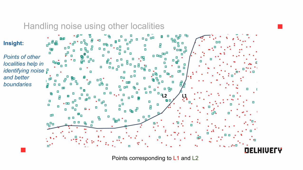
Points corresponding to L1 and L2

L1L2

Insight:

Points of other localities help in identifying noise and better boundaries

How to handle noise?

What is the locality at position X?● We compute the probability that it is L1:

P(L1|X)● We compute the probability that it is L2:

P(L2|X)● X is L1 if P(L1|X) > P(L2|X) else L2

.How to compute P(L1|X)?● Every red point contributes to it

additively● Closer points contribute more than the

distant points

This technique is called KDE and the rule is a kernel. P(L1|X) = 0.95

P(L2|X) = 0.05=> The locality at X is L1

Probability distribution from points

Contribution to spatial probability by a single point

O

O O

O

O O

Contribution to spatial probability by multiple points

Handling noise with probabilities of different localities

Three red points and a green point.

O

O

O

O

The probability due to red points wins over that of the green point.

Optimizations

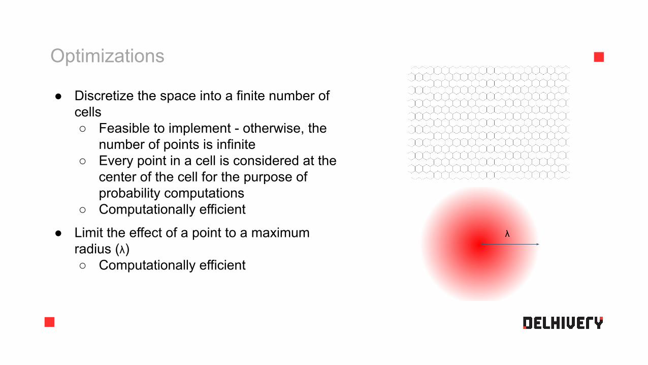
● Discretize the space into a finite number of cells○ Feasible to implement - otherwise, the

number of points is infinite○ Every point in a cell is considered at the

center of the cell for the purpose of probability computations

○ Computationally efficient

λ● Limit the effect of a point to a maximum radius (λ)○ Computationally efficient

End-to-end example

Points corresponding to L1 and L2

Spatial probability distribution of L2

Spatial probability distribution of L1

Final boundary separating L1 and L2

Determining boundaries

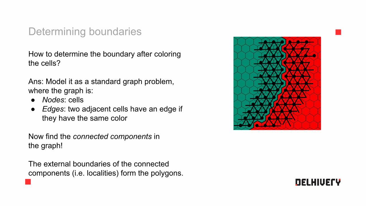
How to determine the boundary after coloring the cells?

Ans: Model it as a standard graph problem, where the graph is:● Nodes: cells● Edges: two adjacent cells have an edge if

they have the same color

Now find the connected components in the graph!

The external boundaries of the connected components (i.e. localities) form the polygons.

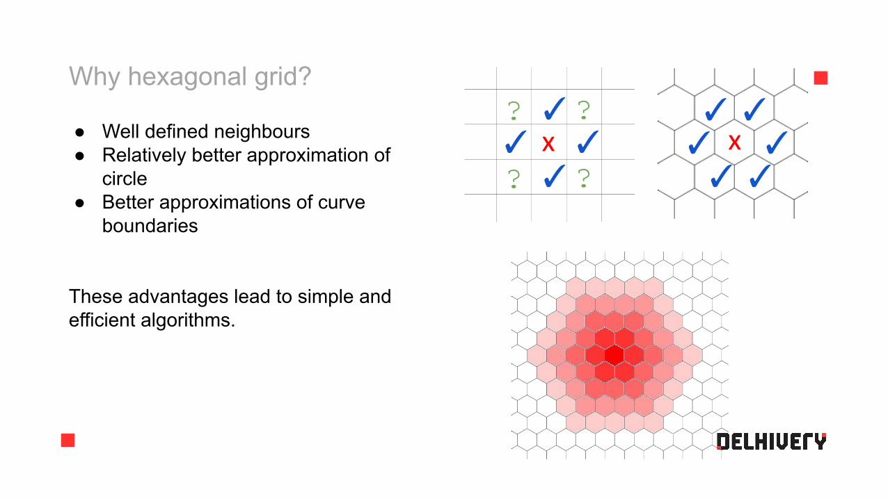
Why hexagonal grid?

● Well defined neighbours● Relatively better approximation of

circle● Better approximations of curve

boundaries

These advantages lead to simple and efficient algorithms.

x ✓✓

✓✓? ?

? ?x✓✓

✓✓

✓✓

Results

Correctness can be checked by comparing the generated polygons with the actual polygons.

Test set:● 21 cities consisting of 1030 localities● True polygons from: OpenStreetMap (OSM), Google Maps● These cities are distributed across the country

○ Northern/central: 9○ Western: 6○ Southern: 4○ Eastern: 2

● These cities are distributed across tiers○ Metropolitan: 7○ tier-1: 6○ tier-2: 8

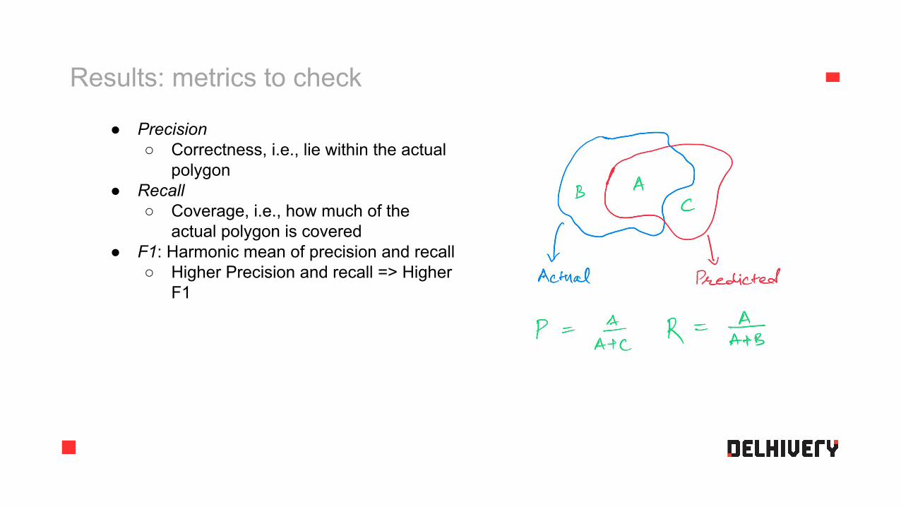
Results: metrics to check

● Precision○ Correctness, i.e., lie within the actual

polygon● Recall

○ Coverage, i.e., how much of the actual polygon is covered

● F1: Harmonic mean of precision and recall○ Higher Precision and recall => Higher

F1

Results

● P-R tradeoff -- with increasing λ: precision ↓ and recall ↑● One can chose the hyperparameter λ based on the use case

λ

5m

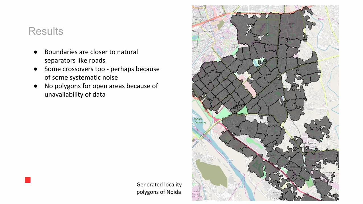
Results

Generated locality polygons of Noida

● Boundaries are closer to natural separators like roads

● Some crossovers too - perhaps because of some systematic noise

● No polygons for open areas because of unavailability of data

Results: PIN Polygon

Polygon of PIN code 600006 of Chennai

Also found cases of PIN codes where the Google Maps polygons are off by 100 kms

Generated polygon

Google Maps polygon

Learning concepts

● Not limited to localities● Can learn polygons of concepts like

DC serviceable area, PIN codes● These polygons can then be used to

create a mapper like service for Geocoder

Gurgaon DC service map

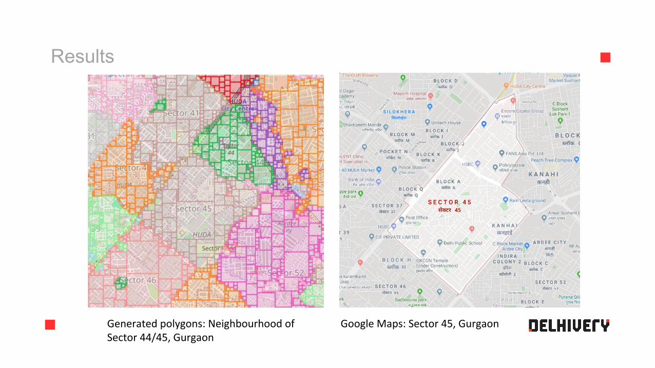
Results

Generated polygons: Neighbourhood of Sector 44/45, Gurgaon

Google Maps: Sector 45, Gurgaon

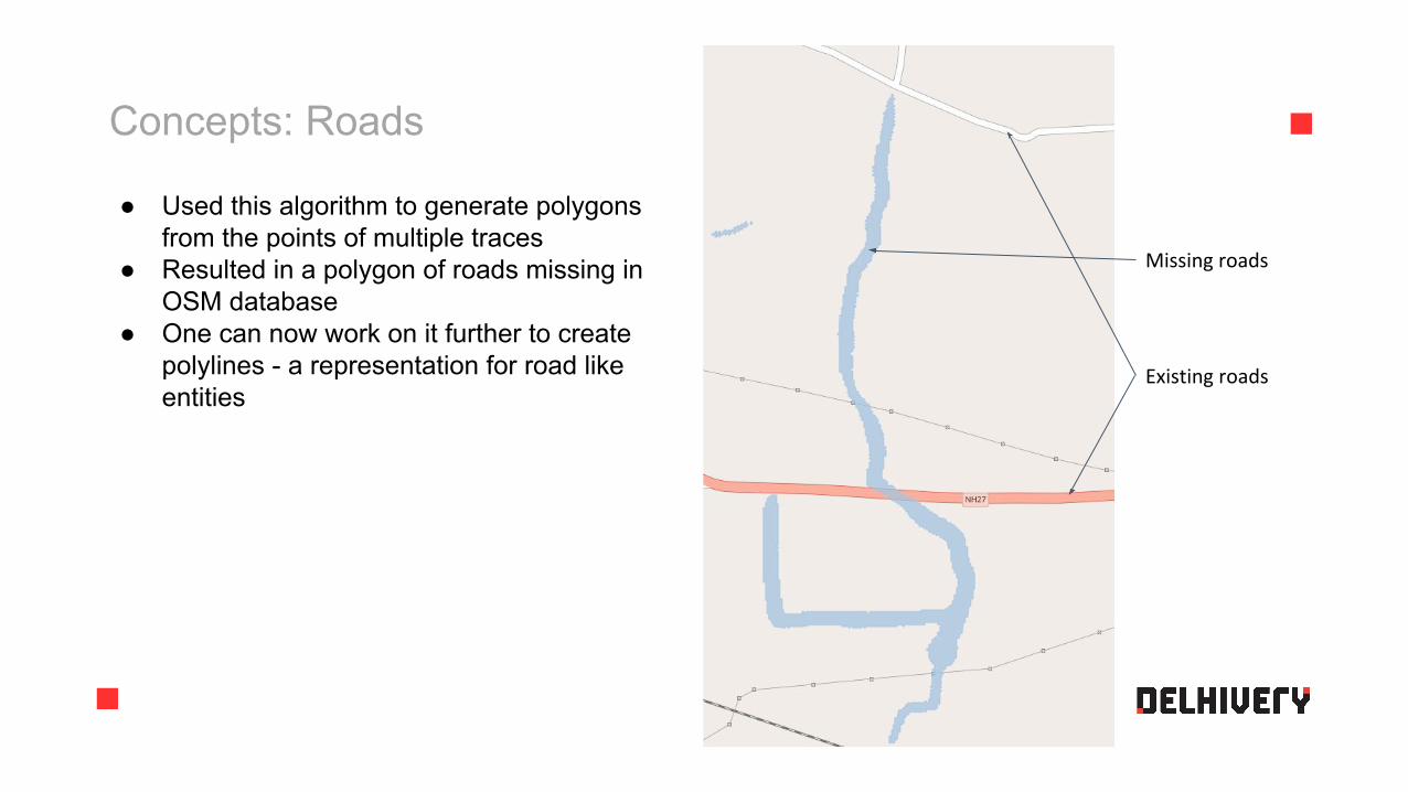
Concepts: Roads

● Used this algorithm to generate polygons from the points of multiple traces

● Resulted in a polygon of roads missing in OSM database

● One can now work on it further to create polylines - a representation for road like entities

Missing roads

Existing roads

Applications using locality maps

● Geofencing of future deliveries● Locality intelligence

○ Time per shipment of every locality● Geocoding of addresses

○ Create polygons of all the entities in addresses○ Then use intersection at the time of prediction to predict the centroid and error

radius

Summary

● Describe the geospatial data produced by e-commerce and logistics operations● The data can be used for learning locality and road maps● Can also be used for learning concepts ● The algorithm can handle noise

Formalism