Embed Size (px)
Citation preview

LEARNING AND TEACHING OF MACROECONOMICS:
AS-AD MODEL & MONEY MARKET ANALYSIS ONLINE COURSE

Reminder
2
The contents of this PPT are for teachers’ knowledge enrichment purpose. Some of the contents are not required in the Economics Curriculum and teachers are not expected to make use of this PPT directly for their daily teaching.

TEACHING AS-AD & MONEY MARKET
MODEL
Fred KUCUHK Business School

OUTLINE
1. Experience sharing on teaching macroeconomics, using ADAS model as an example
2. The effect of tax policies on aggregate supply
3. Money market model
4. Resources and book recommendations
4

PART 1EXPERIENCE
SHARING ON
TEACHING
MACROECONOMICS
DIFFICULTY IN TEACHING MACROECONOMICS
6
One difficulty in teaching macroeconomics is that there are different models to analyse similar issues, and they may not yield the same conclusion.
Another is that there are different assumptions even in the same model
e.g., the slope of SRAS: Upward sloping? Horizontal? (out of syllabus)
It is not always easy and straight-forward to apply macroeconomic models to analyse real cases, given the complexity of the reality and time horizon.
We will start by looking at some general issues and common problems.
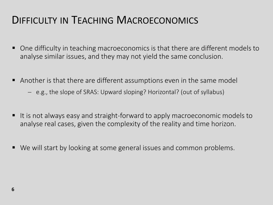
ADAS AS A GRAPHICAL ANALYSISShift vs. Movement along the curve
7
It’s important for students to understand the difference between shifting and movement along the curve. For example:
AD: Yd = C + I + G + NX
Any changes in C, I, and NX induced by changes in price level are represented by a movement along the curve (i.e., the wealth, interest rate, and exchange rate effects)
All other changes are represented by a shift of the AD curve.
Real GDP
Price Level
AD1
•
•
AD2
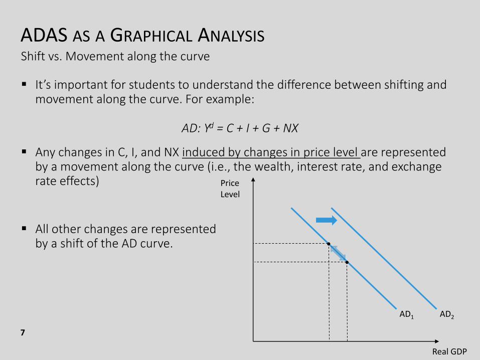
ADAS AS A GRAPHICAL ANALYSISShift vs. Movement along the curve
8
It’s much MORE complicated than demand. It could be quite difficult for some students to understand thoroughly.
Demand (In Microeconomics)
We ask students to distinguish the concepts of DEMAND and QUANTITY DEMANDED
And it’s how they can tell thedifference between shift and movement.
Quantity
Unit Price
D1
•
•
D2
ADAS AS A GRAPHICAL ANALYSISShift vs. Movement along the curve
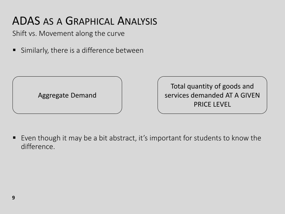
9
Similarly, there is a difference between
Even though it may be a bit abstract, it’s important for students to know the difference.
Aggregate DemandTotal quantity of goods and
services demanded AT A GIVEN PRICE LEVEL
ADAS AS A GRAPHICAL ANALYSISShift vs. Movement along the curve
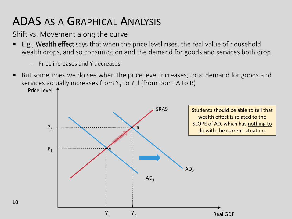
10
E.g., Wealth effect says that when the price level rises, the real value of household wealth drops, and so consumption and the demand for goods and services both drop.
Price increases and Y decreases
But sometimes we do see when the price level increases, total demand for goods and services actually increases from Y1 to Y2! (from point A to B)
Real GDP
Price Level
SRAS
AD1
AD2
Y1
P1A•
Students should be able to tell that wealth effect is related to the
SLOPE of AD, which has nothing to do with the current situation.
B
Y2
P2 •
ADAS AS A GRAPHICAL ANALYSISShift vs. Movement along the curve
11
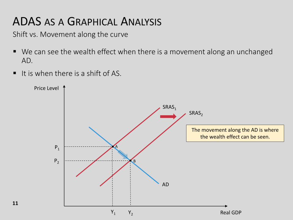
We can see the wealth effect when there is a movement along an unchanged AD.
It is when there is a shift of AS.
Real GDP
Price Level
SRAS1SRAS2
AD
Y1
P1A•
•
Y2
P2 B
The movement along the AD is where the wealth effect can be seen.
ADAS AS A GRAPHICAL ANALYSISShift vs. Movement along the curve
12
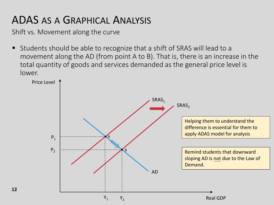
Students should be able to recognize that a shift of SRAS will lead to a movement along the AD (from point A to B). That is, there is an increase in the total quantity of goods and services demanded as the general price level is lower.
Real GDP
Price Level
SRAS1SRAS2
AD
•
Y1 Y2
P2
P1A
B
•
Helping them to understand the difference is essential for them to apply ADAS model for analysis
Remind students that downward sloping AD is not due to the Law of Demand.
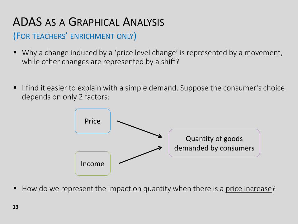
ADAS AS A GRAPHICAL ANALYSIS(FOR TEACHERS’ ENRICHMENT ONLY)
13
Why a change induced by a ‘price level change’ is represented by a movement, while other changes are represented by a shift?
I find it easier to explain with a simple demand. Suppose the consumer’s choice depends on only 2 factors:
How do we represent the impact on quantity when there is a price increase?
Price
Income
Quantity of goods demanded by consumers
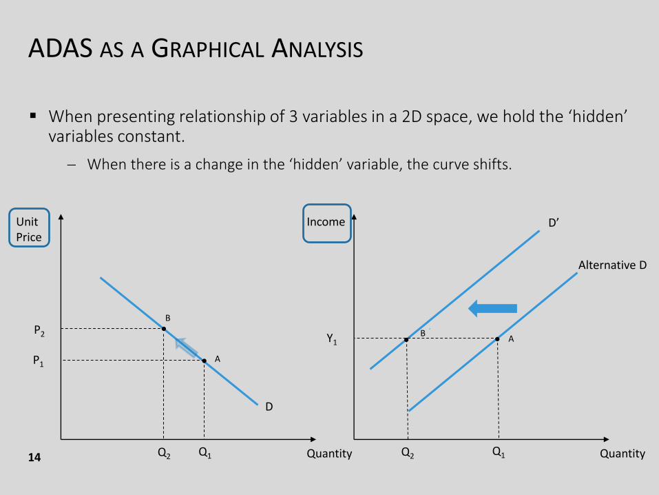
ADAS AS A GRAPHICAL ANALYSIS
14
When presenting relationship of 3 variables in a 2D space, we hold the ‘hidden’ variables constant.
When there is a change in the ‘hidden’ variable, the curve shifts.
Quantity
Unit Price
Quantity
Income
Alternative D
D’
D
• A
Q1
P1
•B
Q2
P2A
Q1
Y1 •
Q2
•B

ADAS AS A GRAPHICAL ANALYSIS
15
Students should know that the ‘shift’ and ‘movement’ depend on the way we present the relationships, and it’s, to certain extent, arbitrary.
The same logic can be applied to aggregate demand and aggregate supply curves.
When there is a change in price level (the variable on Y-axis), then the corresponding change in output will be represented by a movement along the existing curves.
When there is a change in any other (hidden) variable, then the corresponding change in output will be represented by a shift in the curve (i.e., a new curve).
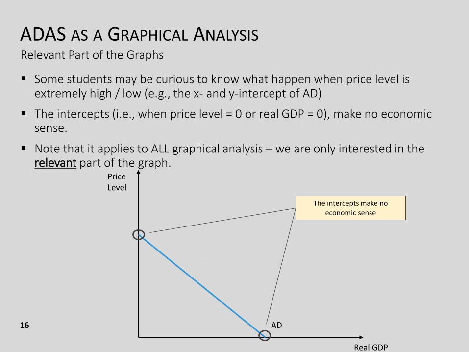
ADAS AS A GRAPHICAL ANALYSISRelevant Part of the Graphs
Some students may be curious to know what happen when price level is extremely high / low (e.g., the x- and y-intercept of AD)
The intercepts (i.e., when price level = 0 or real GDP = 0), make no economic sense.
Note that it applies to ALL graphical analysis – we are only interested in the relevant part of the graph.
Real GDP
Price Level
AD
The intercepts make no economic sense
16
SECONDARY AND OTHER EFFECTS
Generally speaking, the standard analyses that we usually see outline only the major effects of shocks in aggregate demand / supply and govt policies, and how the economy evolves in the long run.
But it does NOT cover everything.
While many students will just follow what you have taught them, it’s often the case that brilliant students may notice something interesting (and make perfect sense sometimes) that you do not plan to cover in the core analysis.
Examples:
Impacts of tax polices on AS
Multiplier effects of fiscal and monetary policies
Stabilizing effect of salaries and profit taxes and social security
17
SECONDARY AND OTHER EFFECTS
It’s often nice to:
Ask him / her to explain the logic clearly, check if it has any SR / LR impacts
Lead him / her to conduct the analysis step by step, if the logic makes sense
Ask him / her to check if it affects the qualitative results (a limitation of graphical analysis like ADAS)
18
SECONDARY AND OTHER EFFECTS
19
In many cases, the qualitative results do not change even if we ignore secondary / other effects.
E.g., whether or not we take into account the multiplier effect of an expansionary fiscal policy, the changes of equilibrium outcome are almost same: AD increases, both price level and output increase
E.g., the effects of automatic stabilizers (social security allowance, salaries and profit tax, etc.) do not affect the major results of analyses
E.g., the slopes of AD and SRAS usually do not matter in qualitative analysis
That’s why we may not want to discuss every detail to keep things manageable.
SECONDARY AND OTHER EFFECTS
20
Some other times, the impacts can be relatively small / neglectable, or do not have a strong consent among economists.
For instance, some economists believe that the impact of salaries tax on laboursupply is small, and what matters more in reality is the labor market regulations
Even though it may be fun, there is no need for us to incorporate that into the fundamental analysis.
Remember that the fundamental ADAS analysis does NOT cover everything, but just outlines the main mechanism that most economists believe.
MORE ON SHORT RUN AGGREGATE SUPPLY
21
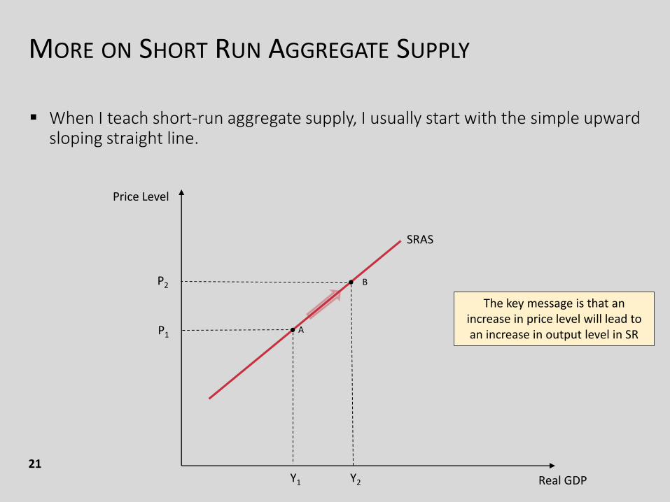
When I teach short-run aggregate supply, I usually start with the simple upward sloping straight line.
Real GDP
Price Level
SRAS
Y1
P1A•
B•
Y2
P2
The key message is that an increase in price level will lead to an increase in output level in SR
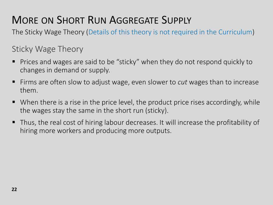
MORE ON SHORT RUN AGGREGATE SUPPLYThe Sticky Wage Theory (Details of this theory is not required in the Curriculum)
Sticky Wage Theory
Prices and wages are said to be “sticky” when they do not respond quickly to changes in demand or supply.
Firms are often slow to adjust wage, even slower to cut wages than to increase them.
When there is a rise in the price level, the product price rises accordingly, while the wages stay the same in the short run (sticky).
Thus, the real cost of hiring labour decreases. It will increase the profitability of hiring more workers and producing more outputs.
22
MORE ON SHORT RUN AGGREGATE SUPPLYThe Sticky Wage Theory (Details of this theory is not required in the Curriculum)
The sticky wage theory help students connect ADAS and what happen in the labour market easily.
While labour market takes some time to adjust, the capital market is usually much more flexible to changes.
Connecting ADAS and labour market help students to understand how policies / changes in labour market may affect the overall economy in SR and LR.
23
MORE ON SHORT RUN AGGREGATE SUPPLYDetails of this theory is not required in the Curriculum
24
In any case, the theories that lead us to an upward sloping SRAS do NOT tell us the specific curvature of the line.
While SRAS as an upward sloping straight line is perfectly fine in many cases (the relevant part)…
It can be quite restrictive in case we want to discuss the impacts of shocks / policies when the economy is close to production capacity.
MORE ON SHORT RUN AGGREGATE SUPPLY(FOR TEACHERS’ ENRICHMENT ONLY)
25
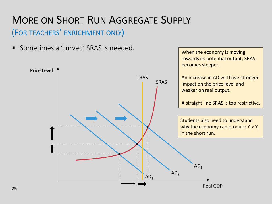
Sometimes a ‘curved’ SRAS is needed.
Real GDP
Price Level
SRAS
AD1
AD2
AD3
•
•
•
LRAS
When the economy is moving towards its potential output, SRAS becomes steeper.
An increase in AD will have stronger impact on the price level and weaker on real output.
A straight line SRAS is too restrictive.
Students also need to understand why the economy can produce Y > Yn
in the short run.
MORE ON SHORT RUN AGGREGATE SUPPLY
26
A SRAS that is an upward sloping straight line is too simple to show these effects.
A natural question from students will be like “when will the SRAS be a straight line, and when will it be a curve?” or “how flat the curve is?”
Unfortunately, no one has a definite answer.
MORE ON SHORT RUN AGGREGATE SUPPLY
27
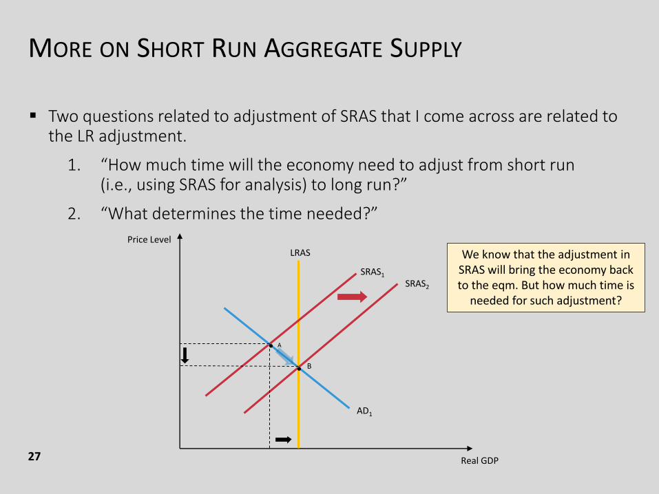
Two questions related to adjustment of SRAS that I come across are related to the LR adjustment.
1. “How much time will the economy need to adjust from short run (i.e., using SRAS for analysis) to long run?”
2. “What determines the time needed?”
Real GDP
Price Level
LRAS
SRAS1
SRAS2
AD1
• A
• B
We know that the adjustment in SRAS will bring the economy back to the eqm. But how much time is
needed for such adjustment?
MORE ON SHORT RUN AGGREGATE SUPPLY
28
Two questions related to adjustment of SRAS that I come across are related to the LR adjustment.
1. “How much time will the economy need to adjust from short run (i.e., using SRAS for analysis) to long run?”
2. “What determines the time needed?”
The short run in macroeconomic analysis is a period in which wages and some other prices do not fully respond to changes in economic conditions.
Under the “Imperfect Adjustment of Input and Output Prices” theory, then the short run is the period in which the input and output prices fails to adjust fully.
The long run is a period in which wages and prices are flexible / can fully adjust.
MORE ON SHORT RUN AGGREGATE SUPPLY
29
There is no magic number (e.g., 3 / 5 years?) that every economists agree.
But generally speaking, we’re usually talking about a period of several years.
It’s often enough to let students have an idea.
What determines the time needed for adjustment?
The more flexible the wages and prices in economy is, the shorter the ‘short run’.
In other words, it depends on how flexible people’s expectation on prices and wages are, as well as adjustment mechanism in the labour market.
E.g, the more rigid the labour market regulations are, the longer the time period it takes for wages to adjust.
So, the longer the time needed for the whole economy to adjust to the long-run equilibrium.

PART 2THE EFFECTS
OF TAX
POLICIES ON
AGGREGATE
SUPPLY
THE EFFECTS OF TAX POLICIES ON AGGREGATE SUPPLY
Tax imposes a difference between the pre-tax and post-tax returns to an economic activity.
When workers, savers, investors, or entrepreneurs change their behavior as a result of a tax change, economists say that there has been a behavioral response to the tax change.
These behavioral responses to the tax change can have important implications on policy and society.
Let’s briefly look at the effects on aggregate supply of cutting some common taxes.
31
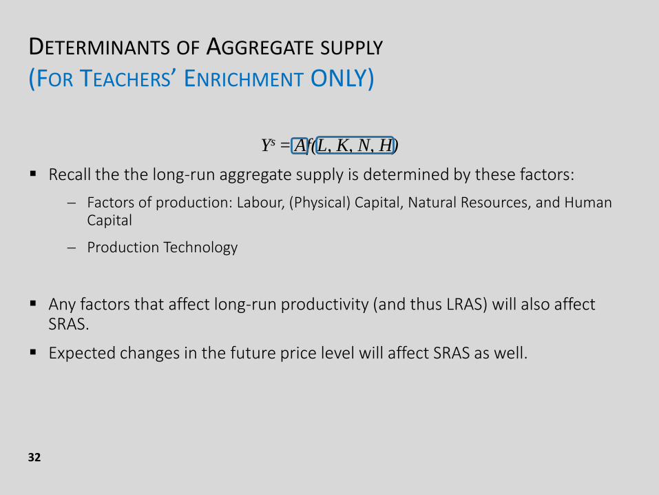
DETERMINANTS OF AGGREGATE SUPPLY
(FOR TEACHERS’ ENRICHMENT ONLY)
Ys = Af(L, K, N, H)
Recall the the long-run aggregate supply is determined by these factors:
Factors of production: Labour, (Physical) Capital, Natural Resources, and Human Capital
Production Technology
Any factors that affect long-run productivity (and thus LRAS) will also affect SRAS.
Expected changes in the future price level will affect SRAS as well.
32
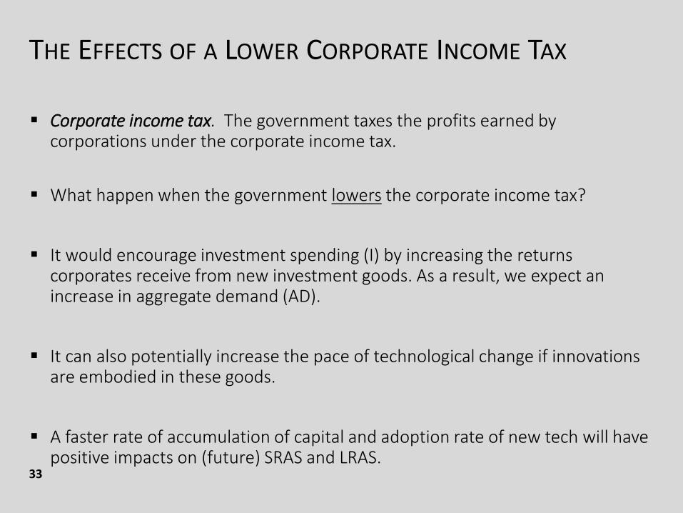
THE EFFECTS OF A LOWER CORPORATE INCOME TAX
Corporate income tax. The government taxes the profits earned by corporations under the corporate income tax.
What happen when the government lowers the corporate income tax?
It would encourage investment spending (I) by increasing the returns corporates receive from new investment goods. As a result, we expect an increase in aggregate demand (AD).
It can also potentially increase the pace of technological change if innovations are embodied in these goods.
A faster rate of accumulation of capital and adoption rate of new tech will have positive impacts on (future) SRAS and LRAS.
33
THE EFFECTS OF A LOWER CORPORATE INCOME TAX
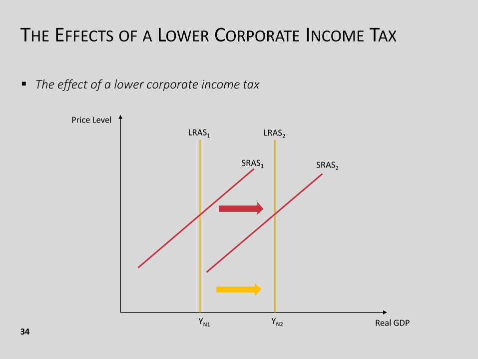
34
The effect of a lower corporate income tax
Real GDP
Price Level
LRAS1 LRAS2
SRAS1 SRAS2
YN1 YN2
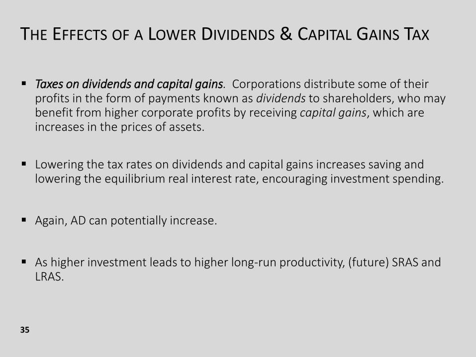
THE EFFECTS OF A LOWER DIVIDENDS & CAPITAL GAINS TAX
Taxes on dividends and capital gains. Corporations distribute some of their profits in the form of payments known as dividends to shareholders, who may benefit from higher corporate profits by receiving capital gains, which are increases in the prices of assets.
Lowering the tax rates on dividends and capital gains increases saving and lowering the equilibrium real interest rate, encouraging investment spending.
Again, AD can potentially increase.
As higher investment leads to higher long-run productivity, (future) SRAS and LRAS.
35
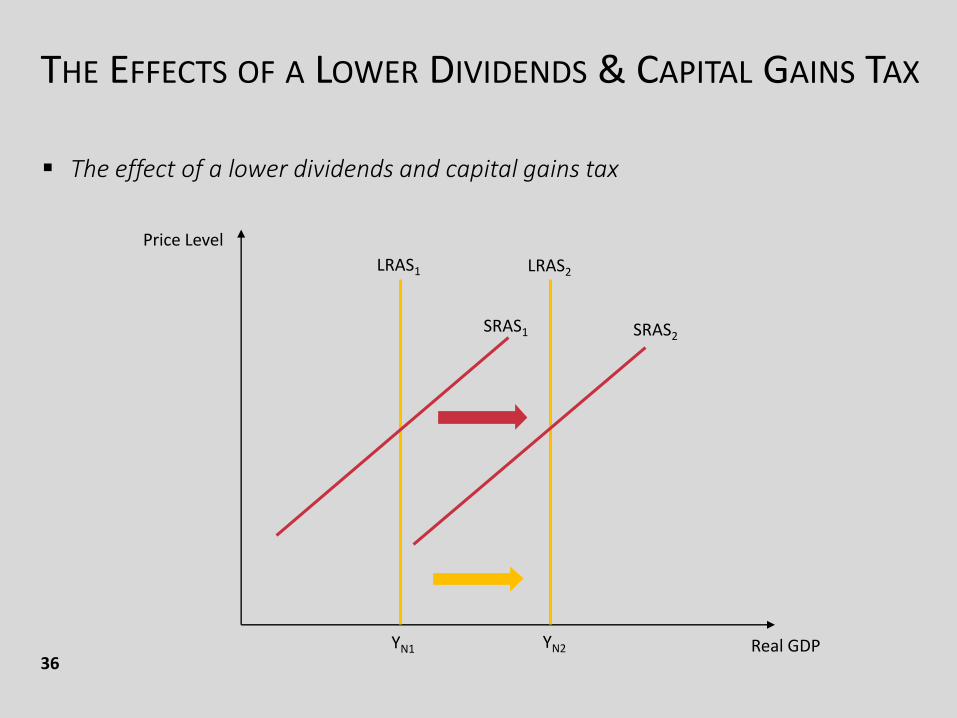
THE EFFECTS OF A LOWER DIVIDENDS & CAPITAL GAINS TAX
36
The effect of a lower dividends and capital gains tax
Real GDP
Price Level
LRAS1 LRAS2
SRAS1 SRAS2
YN1 YN2
THE EFFECTS OF A LOWER SALARIES TAX
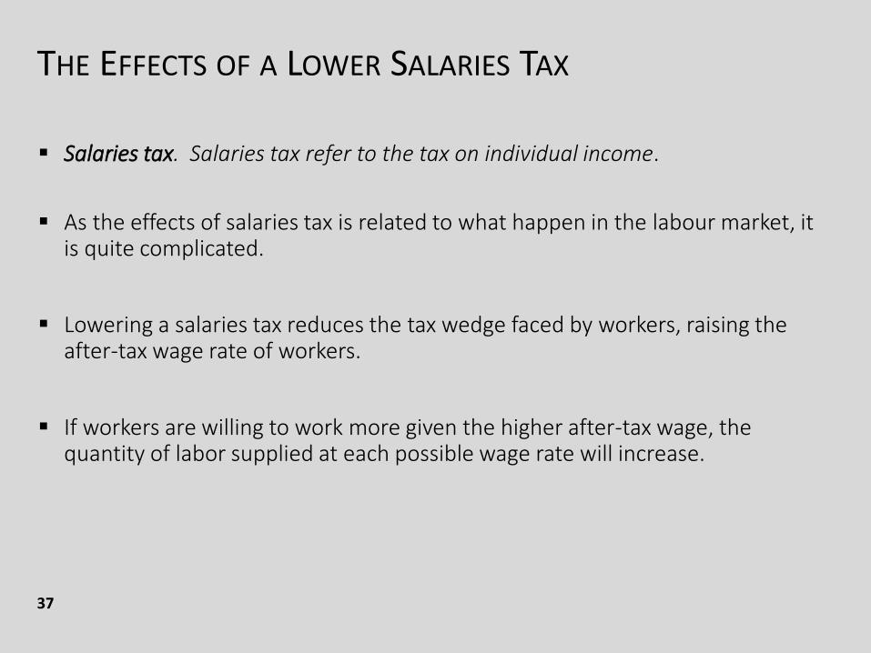
Salaries tax. Salaries tax refer to the tax on individual income.
As the effects of salaries tax is related to what happen in the labour market, it is quite complicated.
Lowering a salaries tax reduces the tax wedge faced by workers, raising the after-tax wage rate of workers.
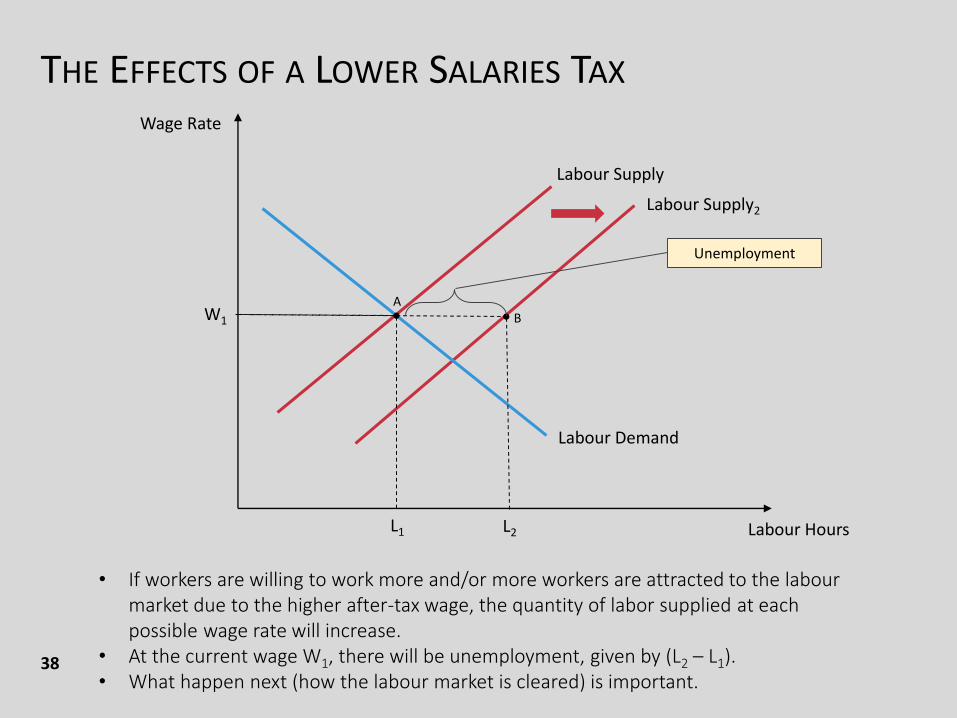
If workers are willing to work more given the higher after-tax wage, the quantity of labor supplied at each possible wage rate will increase.
37
THE EFFECTS OF A LOWER SALARIES TAX
38
Labour Hours
Wage Rate
Labour Supply
Labour Supply2
Labour Demand
•A
B
L1 L2
W1 •
Unemployment
• If workers are willing to work more and/or more workers are attracted to the labourmarket due to the higher after-tax wage, the quantity of labor supplied at each possible wage rate will increase.
• At the current wage W1, there will be unemployment, given by (L2 – L1).• What happen next (how the labour market is cleared) is important.
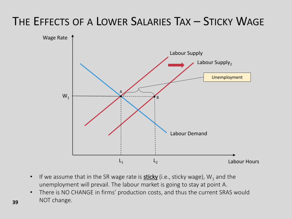
THE EFFECTS OF A LOWER SALARIES TAX – STICKY WAGE
39
Labour Hours
Wage Rate
Labour Supply
Labour Supply2
Labour Demand
•A
B
L1 L2
W1 •
Unemployment
• If we assume that in the SR wage rate is sticky (i.e., sticky wage), W1 and the unemployment will prevail. The labour market is going to stay at point A.
• There is NO CHANGE in firms’ production costs, and thus the current SRAS would NOT change.
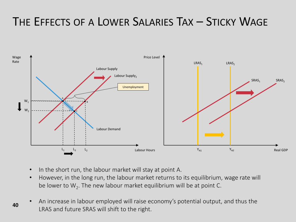
THE EFFECTS OF A LOWER SALARIES TAX – STICKY WAGE
40
Real GDP
Price Level
LRAS1 LRAS2
SRAS1
YN1 YN2Labour Hours
Wage Rate
Labour Supply
Labour Supply2
Labour Demand
•A
B
L1 L2
W1 •
Unemployment
• In the short run, the labour market will stay at point A. • However, in the long run, the labour market returns to its equilibrium, wage rate will
be lower to W2. The new labour market equilibrium will be at point C.
• An increase in labour employed will raise economy’s potential output, and thus the LRAS and future SRAS will shift to the right.
W2 •
L3
C
SRAS2
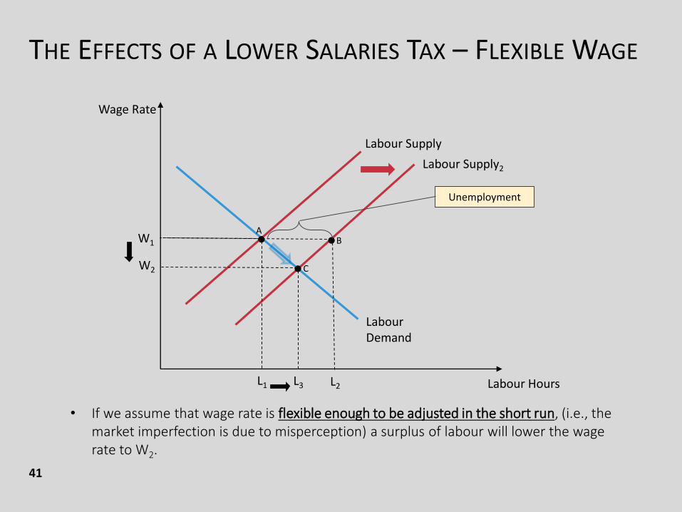
THE EFFECTS OF A LOWER SALARIES TAX – FLEXIBLE WAGE
41
• If we assume that wage rate is flexible enough to be adjusted in the short run, (i.e., the market imperfection is due to misperception) a surplus of labour will lower the wage rate to W2.
Labour Hours
Wage Rate
Labour Supply
Labour Supply2
LabourDemand
•A
B
L1 L2
W1 •
Unemployment
W2 •
L3
C
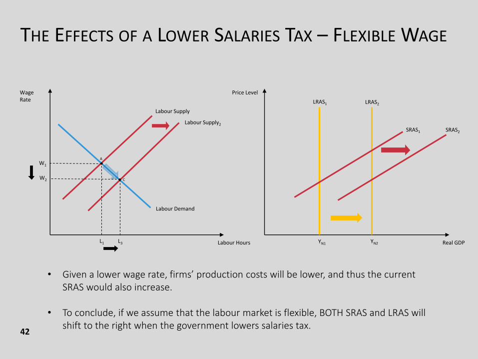
THE EFFECTS OF A LOWER SALARIES TAX – FLEXIBLE WAGE
42
Real GDP
Price Level
LRAS1 LRAS2
SRAS1
YN1 YN2Labour Hours
Wage Rate
Labour Supply
Labour Supply2
Labour Demand
A
L1
W1 •
• Given a lower wage rate, firms’ production costs will be lower, and thus the current SRAS would also increase.
• To conclude, if we assume that the labour market is flexible, BOTH SRAS and LRAS will shift to the right when the government lowers salaries tax.
W2
L3
C
SRAS2
•
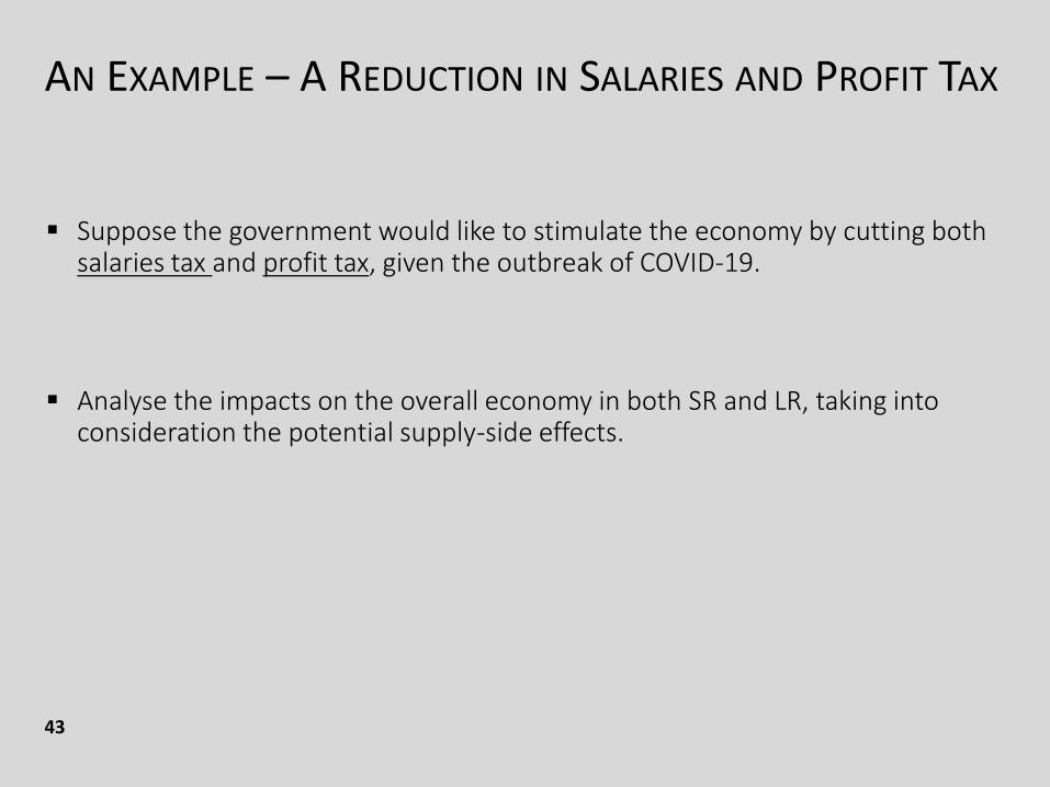
AN EXAMPLE – A REDUCTION IN SALARIES AND PROFIT TAX
43
Suppose the government would like to stimulate the economy by cutting both salaries tax and profit tax, given the outbreak of COVID-19.
Analyse the impacts on the overall economy in both SR and LR, taking into consideration the potential supply-side effects.
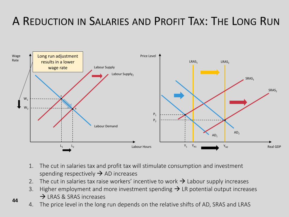
A REDUCTION IN SALARIES AND PROFIT TAX: THE LONG RUN
44
Real GDP
Price Level
LRAS1 LRAS2
SRAS1
Y1 YN2Labour Hours
Wage Rate
Labour Supply
Labour Supply2
Labour Demand
A
L1
W1 •
1. The cut in salaries tax and profit tax will stimulate consumption and investment spending respectively AD increases
2. The cut in salaries tax raise workers’ incentive to work Labour supply increases3. Higher employment and more investment spending LR potential output increases
LRAS & SRAS increases4. The price level in the long run depends on the relative shifts of AD, SRAS and LRAS
W2
L2
B•
Long run adjustment results in a lower
wage rate
AD1
AD2
•P1
P2
SRAS2
•
YN1
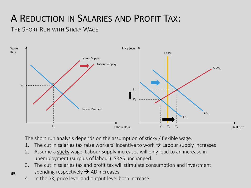
A REDUCTION IN SALARIES AND PROFIT TAX:THE SHORT RUN WITH STICKY WAGE
45
Real GDP
Price Level
LRAS1
SRAS1
YNLabour Hours
Wage Rate
Labour Supply
Labour Demand
A
L1
W1 •
The short run analysis depends on the assumption of sticky / flexible wage.1. The cut in salaries tax raise workers’ incentive to work Labour supply increases2. Assume a sticky wage. Labour supply increases will only lead to an increase in
unemployment (surplus of labour). SRAS unchanged.3. The cut in salaries tax and profit tax will stimulate consumption and investment
spending respectively AD increases4. In the SR, price level and output level both increase.
AD1
AD2
•P1
•
Labour Supply2
P2
Y1 Y2
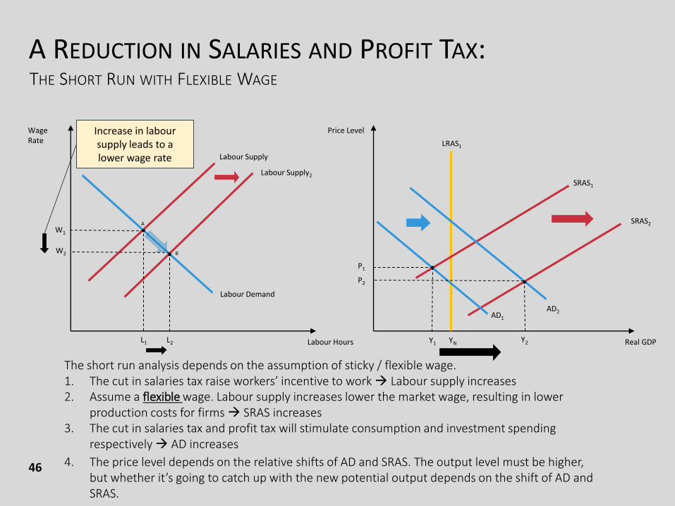
A REDUCTION IN SALARIES AND PROFIT TAX:THE SHORT RUN WITH FLEXIBLE WAGE
46
Real GDP
Price Level
LRAS1
SRAS1
YNLabour Hours
Wage Rate
Labour Supply
Labour Supply2
Labour Demand
A
L1
W1 •
The short run analysis depends on the assumption of sticky / flexible wage.1. The cut in salaries tax raise workers’ incentive to work Labour supply increases2. Assume a flexible wage. Labour supply increases lower the market wage, resulting in lower
production costs for firms SRAS increases3. The cut in salaries tax and profit tax will stimulate consumption and investment spending
respectively AD increases
W2
L2
B
SRAS2
•
Increase in laboursupply leads to a lower wage rate
AD1
AD2
•P1
•
4. The price level depends on the relative shifts of AD and SRAS. The output level must be higher, but whether it’s going to catch up with the new potential output depends on the shift of AD and SRAS.
P2
Y1 Y2

TO SUM UP
47
Let’s summarise our analysis:
1. A reduction in salaries and profit tax will stimulate consumption and investment spending, pushing up aggregate demand.
TO SUM UP
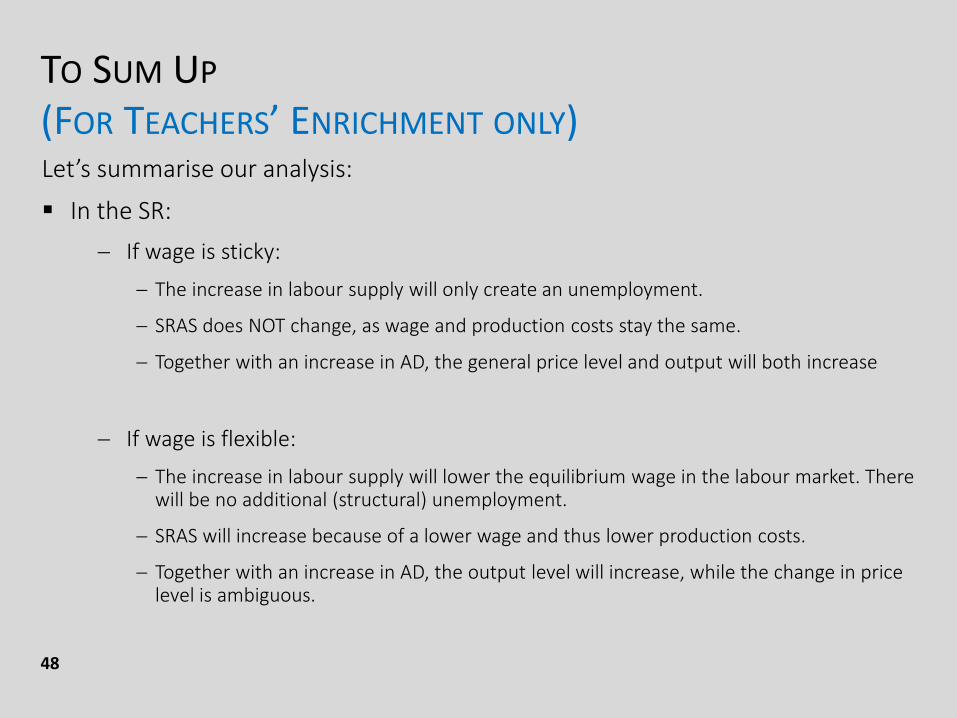
(FOR TEACHERS’ ENRICHMENT ONLY)
48
Let’s summarise our analysis:
In the SR:
If wage is sticky:
The increase in labour supply will only create an unemployment.
SRAS does NOT change, as wage and production costs stay the same.
Together with an increase in AD, the general price level and output will both increase
If wage is flexible:
The increase in labour supply will lower the equilibrium wage in the labour market. There will be no additional (structural) unemployment.
SRAS will increase because of a lower wage and thus lower production costs.
Together with an increase in AD, the output level will increase, while the change in price level is ambiguous.
TO SUM UP
49
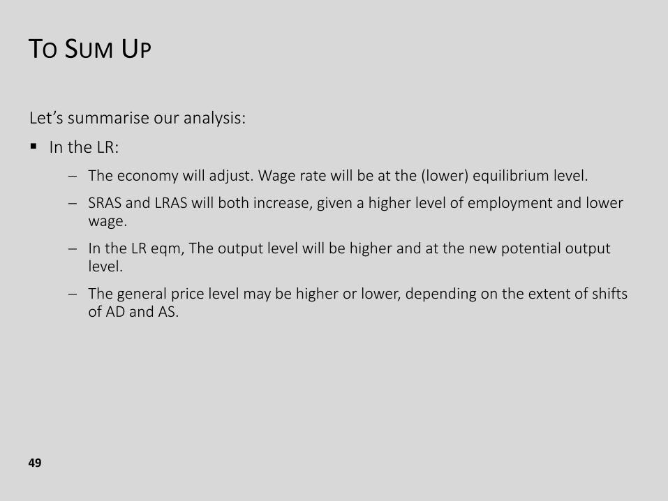
Let’s summarise our analysis:
In the LR:
The economy will adjust. Wage rate will be at the (lower) equilibrium level.
SRAS and LRAS will both increase, given a higher level of employment and lower wage.
In the LR eqm, The output level will be higher and at the new potential output level.
The general price level may be higher or lower, depending on the extent of shifts of AD and AS.
A CLOSER LOOK AT THE LABOUR SUPPLY
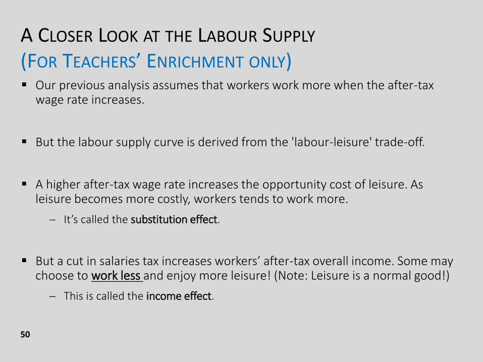
(FOR TEACHERS’ ENRICHMENT ONLY) Our previous analysis assumes that workers work more when the after-tax
wage rate increases.
But the labour supply curve is derived from the 'labour-leisure' trade-off.
A higher after-tax wage rate increases the opportunity cost of leisure. As leisure becomes more costly, workers tends to work more.
It’s called the substitution effect.
But a cut in salaries tax increases workers’ after-tax overall income. Some may choose to work less and enjoy more leisure! (Note: Leisure is a normal good!)
This is called the income effect.
50
A CLOSER LOOK AT THE LABOUR SUPPLY
51
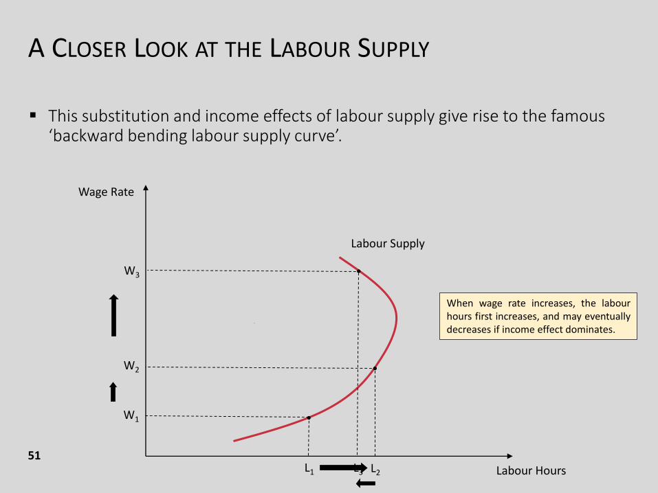
This substitution and income effects of labour supply give rise to the famous ‘backward bending labour supply curve’.
Labour Hours
Wage Rate
Labour Supply
W1
L1
W2 •
L2
•
•W3
L3
When wage rate increases, the labourhours first increases, and may eventuallydecreases if income effect dominates.
A CLOSER LOOK AT THE LABOUR SUPPLY
52
Note that a cut in salaries tax may have a similar effect as increase in market wage rate.
Economists do not have a clear consent about the magnitude of labour supply elasticity.
While many empirical studies suggest a positive relationship between income and quantity of labour supplied, some find it insignificant.
So we’re not quite sure about how labour supply responds to tax changes, especially when it comes to magnitude of changes.
HOW LARGE ARE THESE SUPPLY-SIDE EFFECTS?
Economists who are skeptical of magnitude believe that tax cuts have their greatest effect on aggregate demand rather than on aggregate supply.
There has not a strong consent on the magnitude of supply-side impacts.
53

PART 3MONEY MARKET
MODEL
THE THEORY OF LIQUIDITY PREFERENCE
55
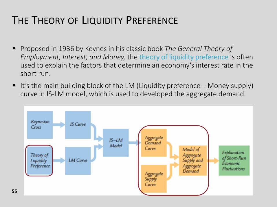
Proposed in 1936 by Keynes in his classic book The General Theory of Employment, Interest, and Money, the theory of liquidity preference is often used to explain the factors that determine an economy’s interest rate in the short run.
It’s the main building block of the LM (Liquidity preference – Money supply) curve in IS-LM model, which is used to developed the aggregate demand.
THE THEORY OF LIQUIDITY PREFERENCE
56
However, it’s not the ONLY model to explain interest rate.
Another very important model is the loanable funds theory (out of syllabus)
The two different theories of the interest rate are useful for different purposes.
Mankiw, Principles of Economics, 8e, p. 742
“When thinking about the long run determinants of the interest rate, it is best to keep in mind the loanable funds theory highlights the importance of an economy’s saving propensities and investment opportunities.”
“When thinking about the short run determinants of the interest rate, it is best to keep in mind the liquidity preference theory, which highlights the importance of monetary policy.”
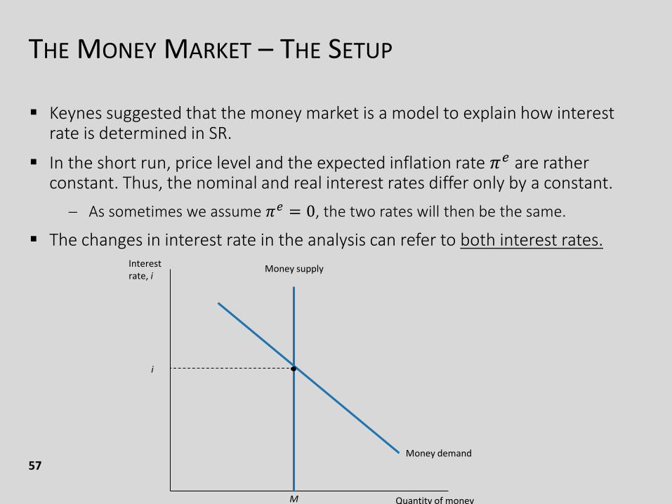
THE MONEY MARKET – THE SETUP
57
Keynes suggested that the money market is a model to explain how interest rate is determined in SR.
In the short run, price level and the expected inflation rate 𝜋𝑒 are rather constant. Thus, the nominal and real interest rates differ only by a constant.
As sometimes we assume 𝜋𝑒 = 0, the two rates will then be the same.
The changes in interest rate in the analysis can refer to both interest rates.Interest rate, i
Quantity of money
Money demand
Money supply
M
i
THE MONEY MARKET – THE SETUP
58
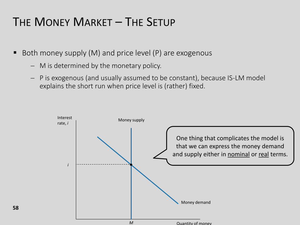
Both money supply (M) and price level (P) are exogenous
M is determined by the monetary policy.
P is exogenous (and usually assumed to be constant), because IS-LM model explains the short run when price level is (rather) fixed.
Interest rate, i
Quantity of money
Money demand
Money supply
M
i
One thing that complicates the model is that we can express the money demand
and supply either in nominal or real terms.
THE MONEY DEMAND
59
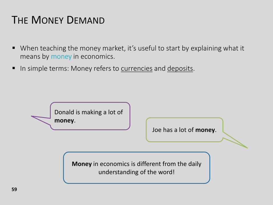
When teaching the money market, it’s useful to start by explaining what it means by money in economics.
In simple terms: Money refers to currencies and deposits.
Donald is making a lot of money.
Joe has a lot of money.
Money in economics is different from the daily understanding of the word!
THE MONEY DEMAND
60
Make it clear to students about the concepts of income, wealth, and money.
Income
What we earn from work, interest and dividends
A flow concept: HK$20,000 per month
Wealth, aka, Financial Wealth
The value of all (financial assets – financial liabilities)
A stock concept: $500,000 as at Dec 2020
The total amount of wealth can be changed over time, via changes income and spending
The composition (form) of wealth can be changedImportant!
THE MONEY DEMAND
61
After understanding these, we can ask students to express the saying more accurately in economic terms:
‘Mary is making a lot of money’ ‘Mary has a high income’
‘Joe has a lot of money’ ‘Joe is wealthy’
THE MONEY DEMAND
62
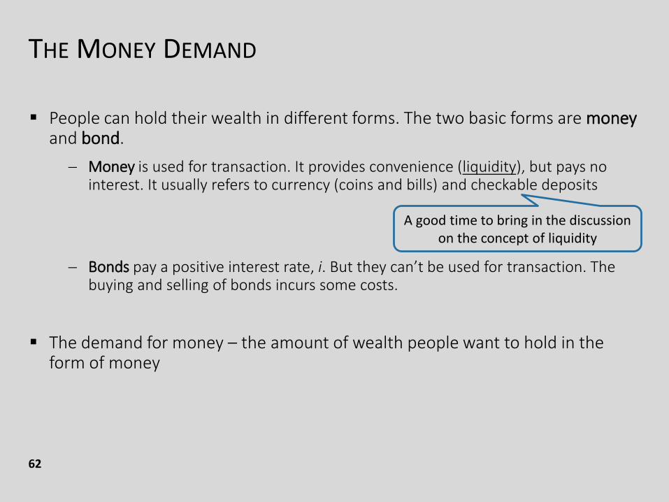
People can hold their wealth in different forms. The two basic forms are moneyand bond.
Money is used for transaction. It provides convenience (liquidity), but pays no interest. It usually refers to currency (coins and bills) and checkable deposits
Bonds pay a positive interest rate, i. But they can’t be used for transaction. The buying and selling of bonds incurs some costs.
The demand for money – the amount of wealth people want to hold in the form of money
A good time to bring in the discussion on the concept of liquidity
THE MONEY DEMAND - DETERMINANTS
63
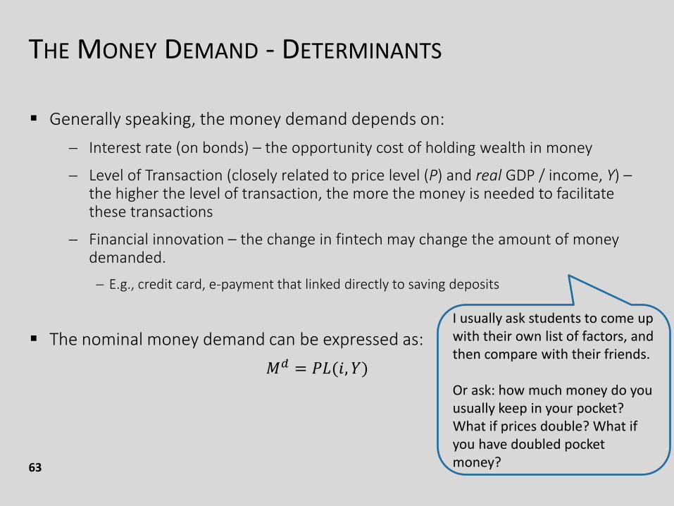
Generally speaking, the money demand depends on:
Interest rate (on bonds) – the opportunity cost of holding wealth in money
Level of Transaction (closely related to price level (P) and real GDP / income, Y) –the higher the level of transaction, the more the money is needed to facilitate these transactions
Financial innovation – the change in fintech may change the amount of money demanded.
E.g., credit card, e-payment that linked directly to saving deposits
The nominal money demand can be expressed as:
𝑀𝑑 = 𝑃𝐿(𝑖, 𝑌)
I usually ask students to come up with their own list of factors, and then compare with their friends.
Or ask: how much money do you usually keep in your pocket? What if prices double? What if you have doubled pocket money?
THE MONEY DEMAND - DETERMINANTS
64
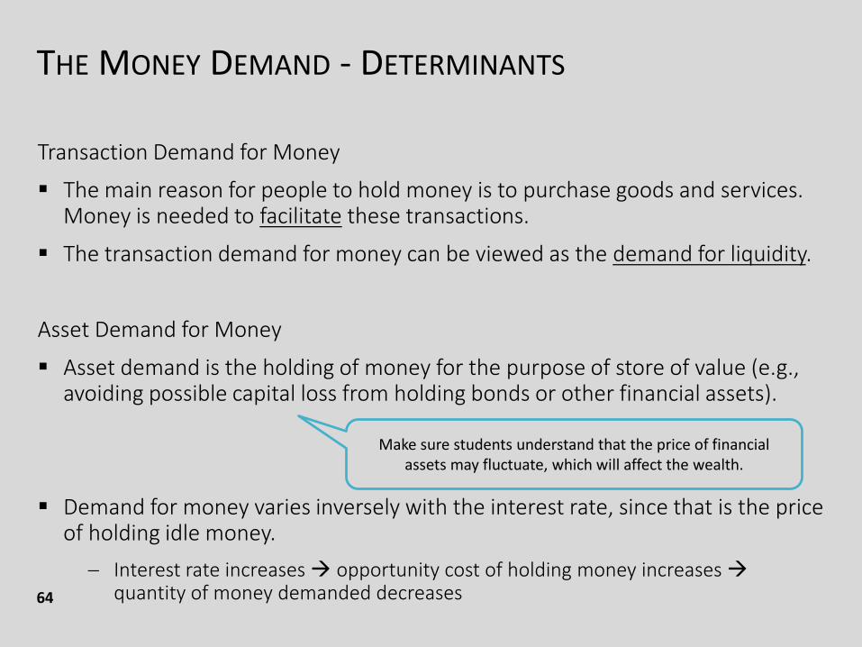
Transaction Demand for Money
The main reason for people to hold money is to purchase goods and services. Money is needed to facilitate these transactions.
The transaction demand for money can be viewed as the demand for liquidity.
Asset Demand for Money
Asset demand is the holding of money for the purpose of store of value (e.g., avoiding possible capital loss from holding bonds or other financial assets).
Demand for money varies inversely with the interest rate, since that is the price of holding idle money.
Interest rate increases opportunity cost of holding money increases quantity of money demanded decreases
Make sure students understand that the price of financial assets may fluctuate, which will affect the wealth.
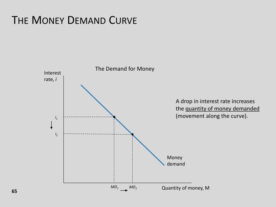
THE MONEY DEMAND CURVE
Interest rate, i
Quantity of money, M
Money demand
The Demand for Money
i1
MD1
i2
MD2
A drop in interest rate increases the quantity of money demanded(movement along the curve).
65
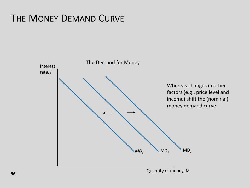
THE MONEY DEMAND CURVE
Interest rate, i
Quantity of money, M
MD1
Whereas changes in other factors (e.g., price level and income) shift the (nominal) money demand curve.
MD2MD3
The Demand for Money
66
THE MONEY DEMAND – REAL AND NOMINAL
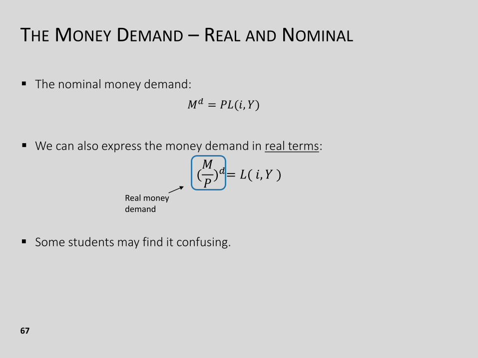
67
The nominal money demand:
𝑀𝑑 = 𝑃𝐿(𝑖, 𝑌)
We can also express the money demand in real terms:
(𝑀
𝑃)𝑑= 𝐿( 𝑖, 𝑌 )
Some students may find it confusing.
Real money demand
THE MONEY DEMAND – REAL AND NOMINAL
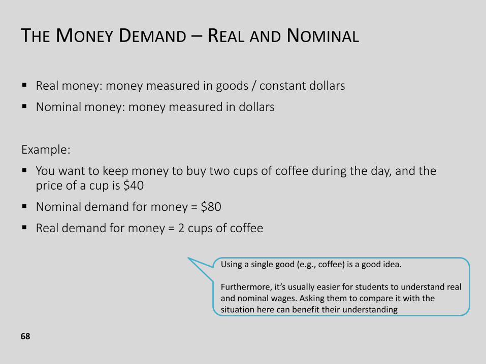
68
Real money: money measured in goods / constant dollars
Nominal money: money measured in dollars
Example:
You want to keep money to buy two cups of coffee during the day, and the price of a cup is $40
Nominal demand for money = $80
Real demand for money = 2 cups of coffee
Using a single good (e.g., coffee) is a good idea.
Furthermore, it’s usually easier for students to understand real and nominal wages. Asking them to compare it with the situation here can benefit their understanding
THE MONEY DEMAND – REAL AND NOMINAL
69
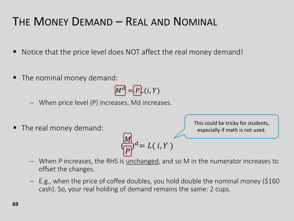
Notice that the price level does NOT affect the real money demand!
The nominal money demand:
𝑀𝑑 = 𝑃𝐿(𝑖, 𝑌)
When price level (P) increases, Md increases.
The real money demand:
(𝑀
𝑃)𝑑= 𝐿( 𝑖, 𝑌 )
When P increases, the RHS is unchanged, and so M in the numerator increases to offset the changes.
E.g., when the price of coffee doubles, you hold double the nominal money ($160 cash). So, your real holding of demand remains the same: 2 cups.
This could be tricky for students, especially if math is not used.
THE MONEY DEMAND – REAL AND NOMINAL
70
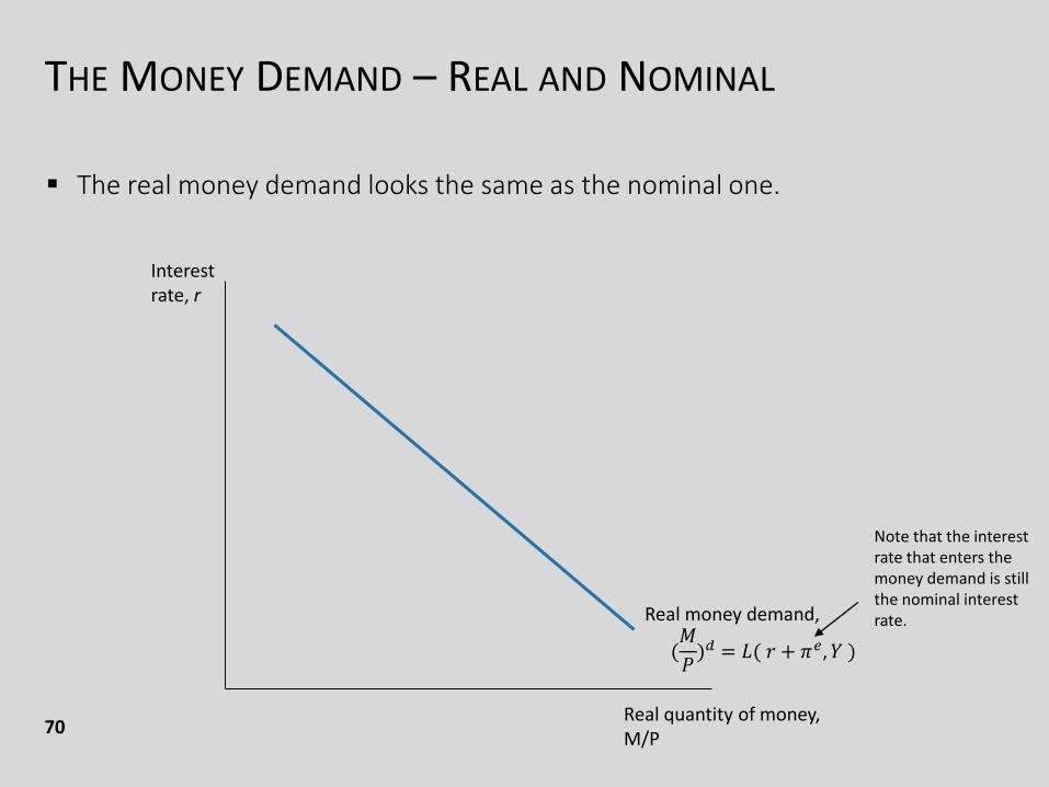
The real money demand looks the same as the nominal one.
Interest rate, r
Real quantity of money, M/P
Real money demand,
(𝑀
𝑃)𝑑 = 𝐿( 𝑟 + 𝜋𝑒, 𝑌 )
Note that the interest rate that enters the money demand is still the nominal interest rate.
THE MONEY SUPPLY – REAL AND NOMINAL
71
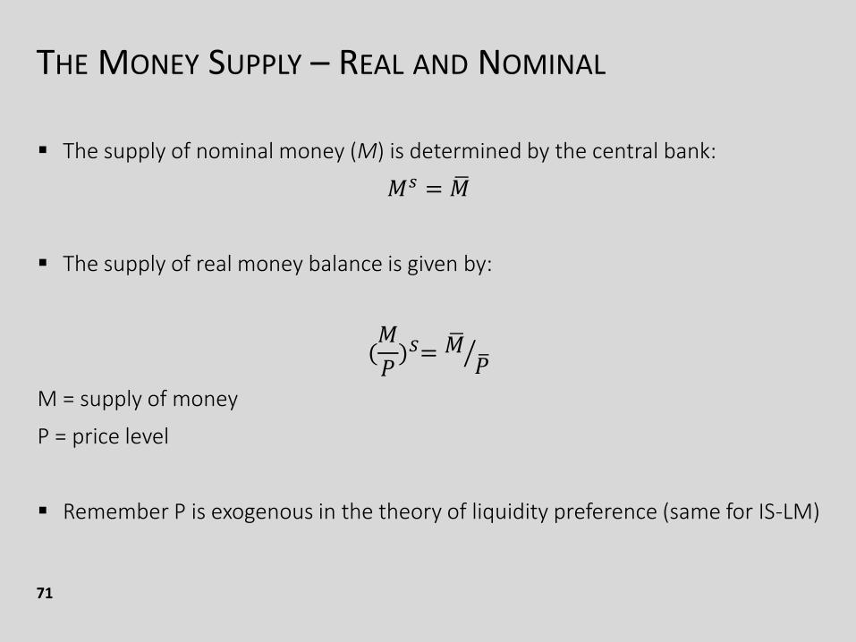
The supply of nominal money (M) is determined by the central bank:
𝑀𝑠 = ഥ𝑀
The supply of real money balance is given by:
(𝑀
𝑃)𝑆= ൗ
ഥ𝑀ത𝑃
M = supply of money
P = price level
Remember P is exogenous in the theory of liquidity preference (same for IS-LM)
THE MONEY SUPPLY – REAL AND NOMINAL
72
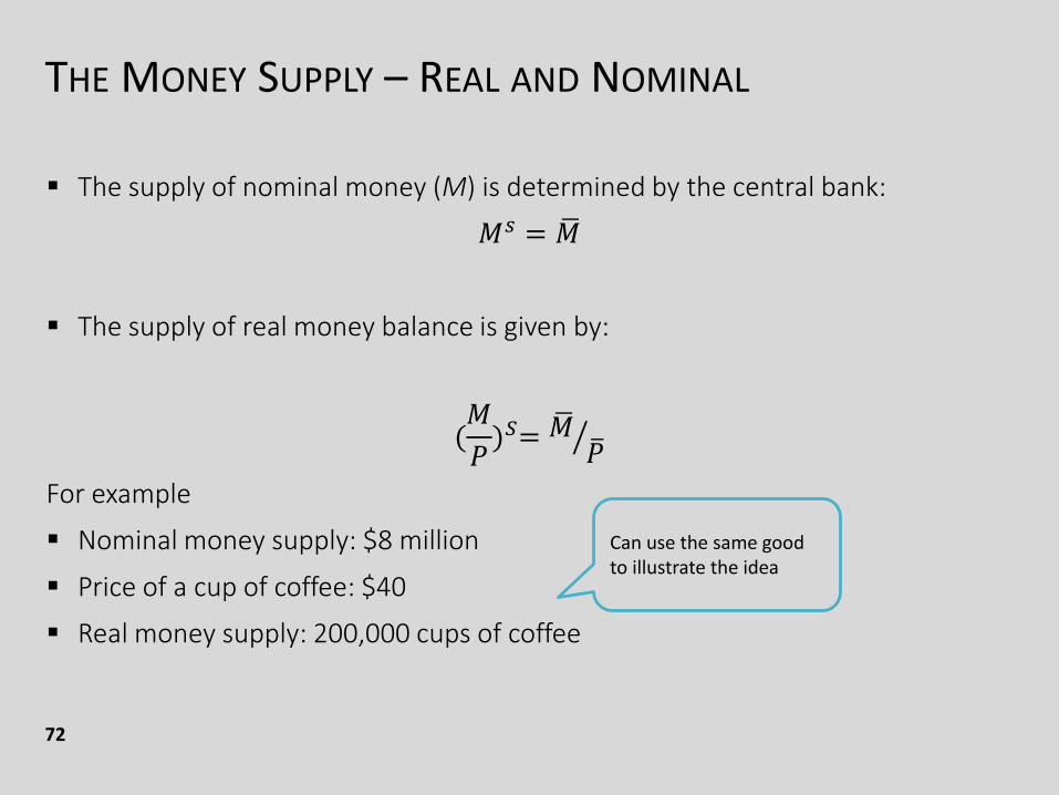
The supply of nominal money (M) is determined by the central bank:
𝑀𝑠 = ഥ𝑀
The supply of real money balance is given by:
(𝑀
𝑃)𝑆= ൗ
ഥ𝑀ത𝑃
For example
Nominal money supply: $8 million
Price of a cup of coffee: $40
Real money supply: 200,000 cups of coffee
Can use the same good to illustrate the idea
THE MONEY SUPPLY – REAL AND NOMINAL
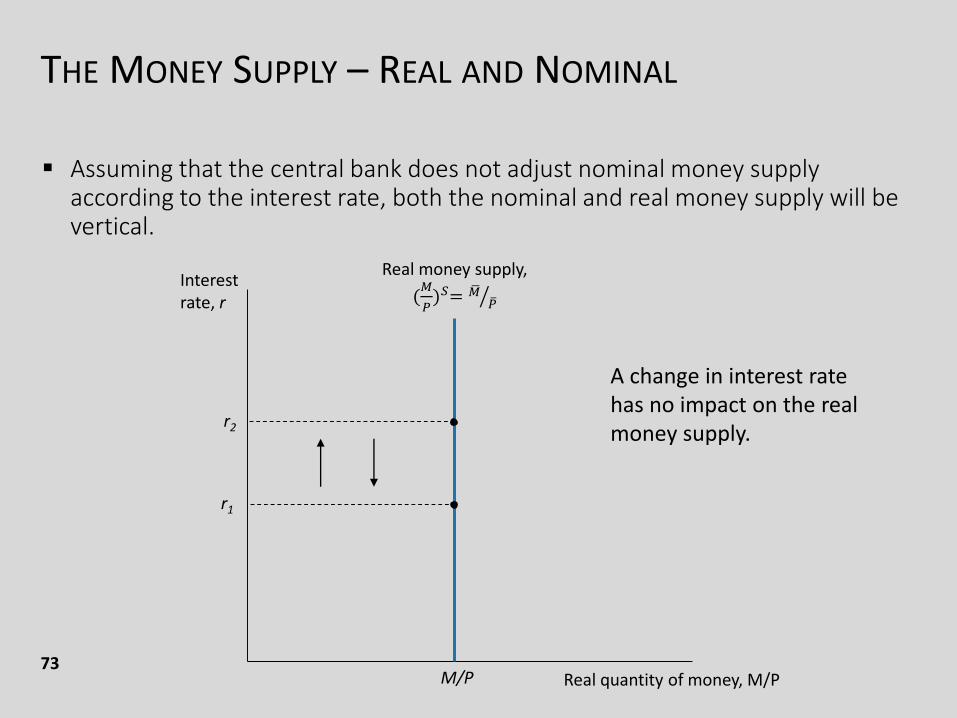
73
Assuming that the central bank does not adjust nominal money supply according to the interest rate, both the nominal and real money supply will be vertical.
Interest rate, r
Real quantity of money, M/P
Real money supply,
(𝑀
𝑃)𝑆= ൗഥ𝑀 ത𝑃
r1
M/P
r2
A change in interest rate has no impact on the real money supply.
THE MONEY SUPPLY
74
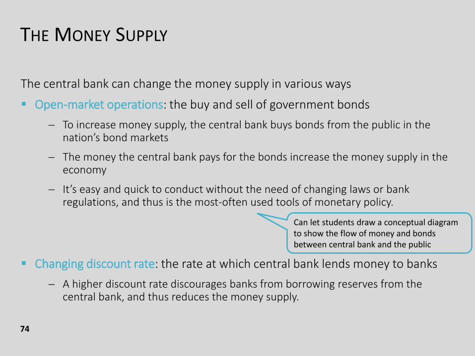
The central bank can change the money supply in various ways
Open-market operations: the buy and sell of government bonds
To increase money supply, the central bank buys bonds from the public in the nation’s bond markets
The money the central bank pays for the bonds increase the money supply in the economy
It’s easy and quick to conduct without the need of changing laws or bank regulations, and thus is the most-often used tools of monetary policy.
Changing discount rate: the rate at which central bank lends money to banks
A higher discount rate discourages banks from borrowing reserves from the central bank, and thus reduces the money supply.
Can let students draw a conceptual diagram to show the flow of money and bonds between central bank and the public
THE MONEY SUPPLY
75
The central bank can change the money supply in various ways
Changing reserve requirement:
An increase in reserve requirements raises the reserve ratio, lowering the money multiplier and decreases the money supply.
It’s only rarely used because such changes disrupt the business of banking.
It will be less effective when banks hold excess reserve.
Paying interest on reserves:
Traditionally, banks did not earn any interest on its reserve at the central bank.
But starting from 2008, the Fed began paying interest on the reserves.
A higher interest rate on reserves, the more reserves banks will choose to hold at the central bank, lowering the money multiplier and decreases the money supply.
It gives the Fed another tool to control the money supply.
THE MONEY SUPPLY
76
We should point out to students that the central bank’s control over money supply is not precise.
The main reason is the fractional-reserve banking system.
1. The central bank cannot control the amount of money that households choose to hold as deposits in banks.
If people lose confidence in the banking system and withdraw deposits to hold more currency, the banking system loses reserves and creates less money.
2. The central bank cannot control the amount that bankers choose to lend.
If bankers become more cautious and make fewer loans, the banking system will create less money, and money supply falls.
But we often simplify the situation by assuming that the central bank can control the money supply precisely. (The difference between theory and reality)
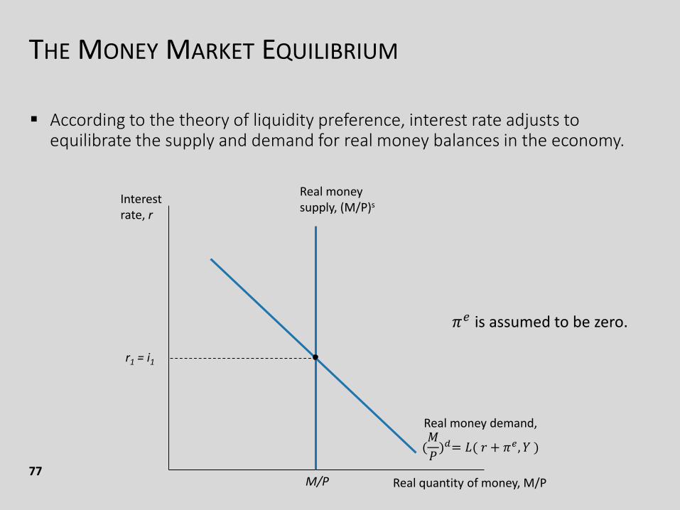
THE MONEY MARKET EQUILIBRIUM
77
According to the theory of liquidity preference, interest rate adjusts to equilibrate the supply and demand for real money balances in the economy.
Interest rate, r
Real quantity of money, M/P
Real money demand,
(𝑀
𝑃)𝑑= 𝐿( 𝑟 + 𝜋𝑒, 𝑌 )
Real money supply, (M/P)s
r1 = i1
M/P
𝜋𝑒 is assumed to be zero.
THE MONEY MARKET EQUILIBRIUM – THE MECHANISM
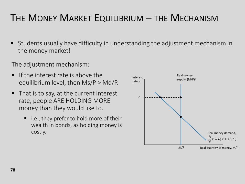
78
Students usually have difficulty in understanding the adjustment mechanism in the money market!
The adjustment mechanism:
If the interest rate is above the equilibrium level, then Ms/P > Md/P.
That is to say, at the current interest rate, people ARE HOLDING MORE money than they would like to.
i.e., they prefer to hold more of their wealth in bonds, as holding money is costly.
r
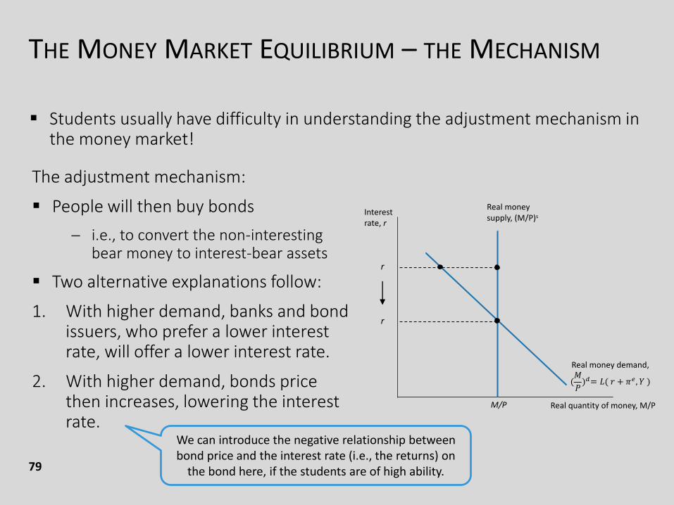
THE MONEY MARKET EQUILIBRIUM – THE MECHANISM
79
Students usually have difficulty in understanding the adjustment mechanism in the money market!
The adjustment mechanism:
People will then buy bonds
i.e., to convert the non-interesting bear money to interest-bear assets
Two alternative explanations follow:
1. With higher demand, banks and bond issuers, who prefer a lower interest rate, will offer a lower interest rate.
2. With higher demand, bonds price then increases, lowering the interest rate.
r
r
We can introduce the negative relationship between bond price and the interest rate (i.e., the returns) on
the bond here, if the students are of high ability.
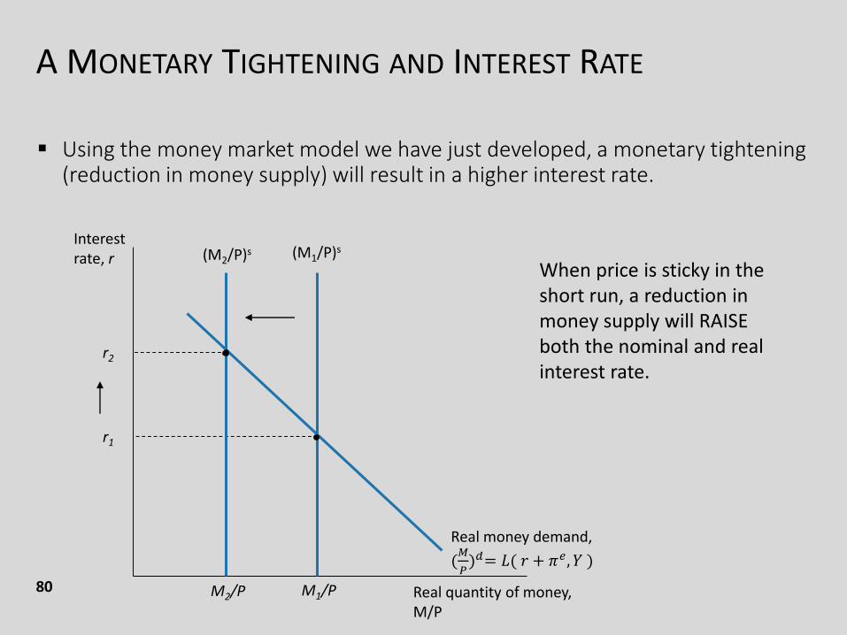
A MONETARY TIGHTENING AND INTEREST RATE
80
Using the money market model we have just developed, a monetary tightening (reduction in money supply) will result in a higher interest rate.
Interest rate, r
Real quantity of money, M/P
Real money demand,
(𝑀
𝑃)𝑑= 𝐿( 𝑟 + 𝜋𝑒, 𝑌 )
(M1/P)s
M1/P
(M2/P)s
M2/P
r1
r2
When price is sticky in the short run, a reduction in money supply will RAISE both the nominal and real interest rate.
A MONETARY TIGHTENING AND AGGREGATE DEMAND
81
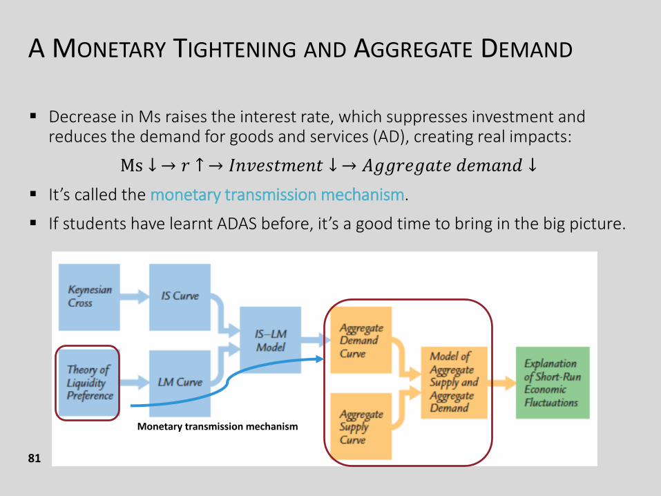
Decrease in Ms raises the interest rate, which suppresses investment and reduces the demand for goods and services (AD), creating real impacts:
Ms ↓ → 𝑟 ↑ → 𝐼𝑛𝑣𝑒𝑠𝑡𝑚𝑒𝑛𝑡 ↓ → 𝐴𝑔𝑔𝑟𝑒𝑔𝑎𝑡𝑒 𝑑𝑒𝑚𝑎𝑛𝑑 ↓
It’s called the monetary transmission mechanism.
If students have learnt ADAS before, it’s a good time to bring in the big picture.
Monetary transmission mechanism
A MONETARY TIGHTENING AND OUTPUT
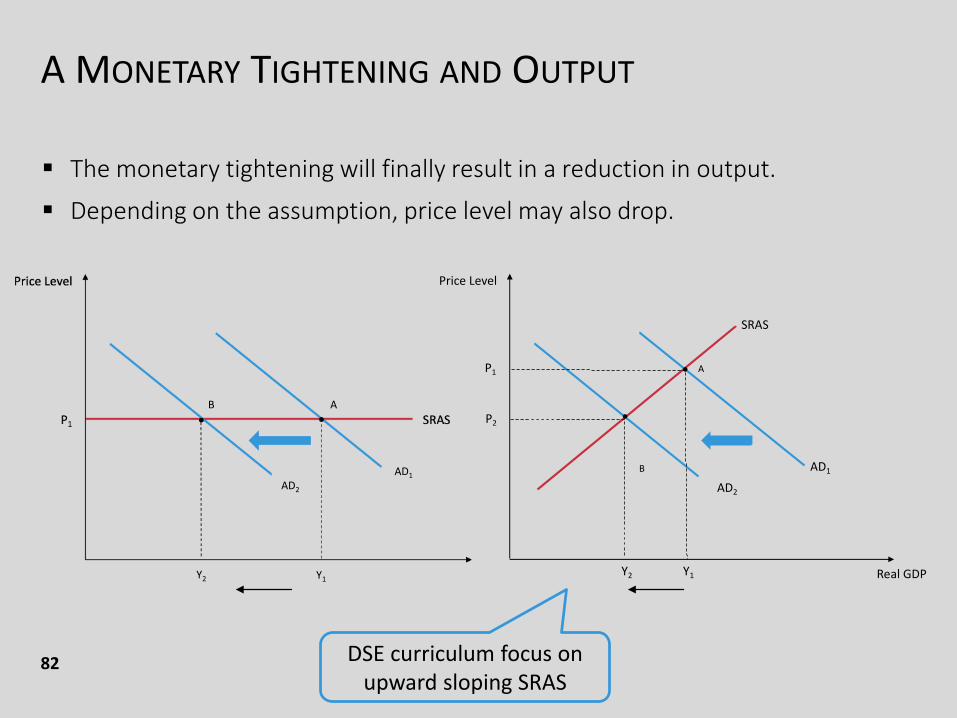
82
The monetary tightening will finally result in a reduction in output.
Depending on the assumption, price level may also drop.
AB
AD1
AD2
Y1Y2 Real GDP
Price Level
SRAS
AD2
AD1
Y2
P2
A
•
B
Y1
P1 •
DSE curriculum focus on upward sloping SRAS
A MONETARY TIGHTENING AND INTEREST RATE - LR
83
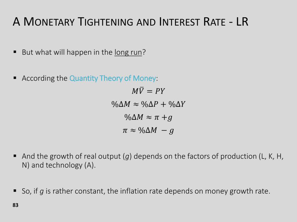
But what will happen in the long run?
According the Quantity Theory of Money:
𝑀ത𝑉 = 𝑃𝑌
%Δ𝑀 ≈%Δ𝑃 +%Δ𝑌
%Δ𝑀 ≈ 𝜋 +𝑔
𝜋 ≈%Δ𝑀 − 𝑔
And the growth of real output (g) depends on the factors of production (L, K, H, N) and technology (A).
So, if g is rather constant, the inflation rate depends on money growth rate.
A MONETARY TIGHTENING AND INTEREST RATE - LR
84
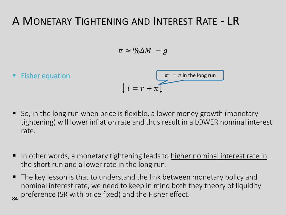
𝜋 ≈%Δ𝑀 − 𝑔
Fisher equation
𝑖 = 𝑟 + 𝜋
So, in the long run when price is flexible, a lower money growth (monetary tightening) will lower inflation rate and thus result in a LOWER nominal interest rate.
In other words, a monetary tightening leads to higher nominal interest rate in the short run and a lower rate in the long run.
The key lesson is that to understand the link between monetary policy and nominal interest rate, we need to keep in mind both they theory of liquidity preference (SR with price fixed) and the Fisher effect.
𝜋𝑒 = 𝜋 in the long run
A MONETARY EXPANSION
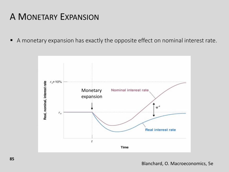
85
A monetary expansion has exactly the opposite effect on nominal interest rate.
Blanchard, O. Macroeconomics, 5e
Monetaryexpansion
A MONETARY EXPANSION
86
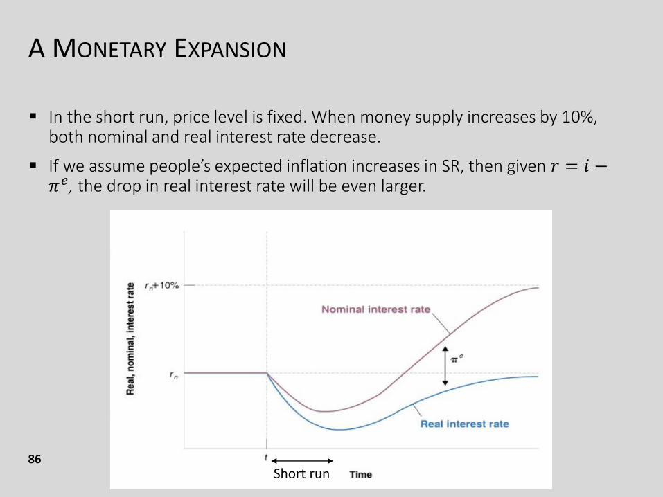
In the short run, price level is fixed. When money supply increases by 10%, both nominal and real interest rate decrease.
If we assume people’s expected inflation increases in SR, then given 𝑟 = 𝑖 −𝜋𝑒, the drop in real interest rate will be even larger.
Short run
A MONETARY EXPANSION
87
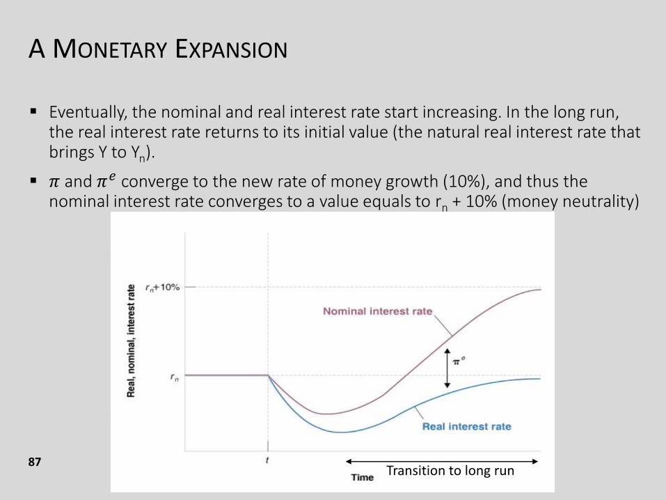
Eventually, the nominal and real interest rate start increasing. In the long run, the real interest rate returns to its initial value (the natural real interest rate that brings Y to Yn).
𝜋 and 𝜋𝑒 converge to the new rate of money growth (10%), and thus the nominal interest rate converges to a value equals to rn + 10% (money neutrality)
Transition to long run
THE NATURAL REAL INTEREST RATE (OUT OF SYLLABUS)
88
The goods market equilibrium is achieved when production Y equals to the total demand for goods: C + I + G.
So, the equilibrium, or the IS curve, is:
𝑌 = 𝐶 𝑌 − 𝑇 + 𝐼 𝑌, 𝑟 + 𝐺
The natural rate of interest, rn, is such that, given T and G, Y = Yn:
𝑌𝑛 = 𝐶 𝑌𝑛 − 𝑇 + 𝐼 𝑌𝑛, 𝑟 + 𝐺
‘In the medium run, the real interest rate returns to the natural interest rate, rn. It is independent of the rate of money growth.’
Blanchard, O. Macroeconomics, 5e, p. 321
THE NATURAL REAL INTEREST RATE (OUT OF SYLLABUS)
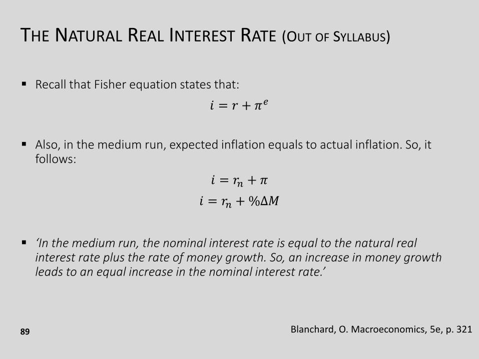
89
Recall that Fisher equation states that:
𝑖 = 𝑟 + 𝜋𝑒
Also, in the medium run, expected inflation equals to actual inflation. So, it follows:
𝑖 = 𝑟𝑛 + 𝜋
𝑖 = 𝑟𝑛 +%∆𝑀
‘In the medium run, the nominal interest rate is equal to the natural real interest rate plus the rate of money growth. So, an increase in money growth leads to an equal increase in the nominal interest rate.’
Blanchard, O. Macroeconomics, 5e, p. 321
CENTRAL BANK’S POLICY INSTRUMENT
90
If students are aware of the news, they should have heard something like “People’s Bank of China or Fed has raised or lowered interest rates”.
But our discussion of money market and ADAS often assume that the central bank influences the economy by controlling the money supply.
It’s important to explain to student this ‘inconsistency’.
In reality, usually central banks use the interest rate as the policy instrument and conduct open-market operation (OMO) to hit the target.
These OMOs will change the money supply so that the equilibrium interest rate equals the target interest rate that the central banks have chosen.
CENTRAL BANK’S POLICY INSTRUMENT
91
As a result of these procedures, central banks policies are often discussed in terms of changing interest rate.
So, it’s nice to remind students, however, that behind these changes in interest rates are the necessary changes in the money supply.
For example
A news saying ‘the Fed has lowered interest rate’ should be understood as ‘the Fed has decided to buy bonds in the open-market operations so as to increase the money supply and reduce the equilibrium interest rate to hit a new lower target’.
CENTRAL BANK’S POLICY INSTRUMENT
92
Possible reasons for using the interest rate include:
Interest rate directly affect economic activities – like investment and borrowing.
The central bank cannot control money supply precisely.
Interest rate is easier to measure
There are different measures of money supply: M1, M2 and so on, and sometimes they move in different directions.
Rather than deciding which measure is the best, central bank avoids the question by using the interest rate as a policy instrument.

PART 4RESOURCES & BOOK
RECOMMENDATION

ONLINE VIDEO RESOURCES
94
反轉經濟教室計劃 - 經士柏 EconsPark
https://www.youtube.com/channel/UCjG8kcfTiiLSrho89owF7vA
Micro and macro economics, available in both English and Cantonese

ONLINE VIDEO RESOURCES
95
Marginal Revolution University - George Mason University
https://mru.org/learn
More than 900 videos and other T&L resources
Available in English

ONLINE VIDEO RESOURCES
96
手說經濟 Economics on Hand
https://www.youtube.com/playlist?list=PLsPSPidSdKo89WD86v4J76chHVw3ZPgh5
49 videos on MC questions, available in both Cantonese and sign language

INTERESTING BOOK TITLES
97
哈佛經濟學家推理系列 -- 《致命的均衡》《邊際謀殺》《奪命曲線》
這三本經濟學推理小說,是由兩位美國經濟學教授所合寫的,是經濟學界絕無僅有的大膽嘗試。三本書共同的主角是哈佛大學的經濟學教授亨利‧史匹曼,他在書中將遭遇離奇的兇殺案,而運用經濟學的常識推理,漂亮破案。

INTERESTING BOOK TITLES
98
為調查在加勒比海聖約翰島上的謀殺案,哈佛大學經濟學教授亨利.史匹曼從「理性」這個主題變化出許多經濟概念並加以應用,其中包括:
★理性的人在選擇「工作」或「休閒」時的思考方式;★如何為一本書訂定最適售價;★為什麼有些人會和別人保持著某種關係;★一個產品的供給量和銷售量在什麼情況下會相等;★不同個人的效用無法比較。
當史匹曼看見有人的行為似乎不太理性,不是以表面上最低的成本來達到目標,他就知道其中必有蹊蹺,只要充分觀察這些「非理性」的行為,他就能推論出對方葫蘆裡賣什麼藥。
https://qrgo.page.link/qvPze

INTERESTING BOOK TITLES
99
經濟自然學 The Economic Naturalist
為什麼牛奶多以長方形容器出售,而一般飲料容器則為圓柱形?
為何硬幣的人頭像多為側面,而紙鈔則是正面肖像?
為什麼高速公路北上車道發生車禍,分隔島對面的南下車道也會塞車?
為什麼開車可以吃漢堡或喝咖啡,講手機卻違法?
所謂「經濟自然學」,就是以生物學界自然觀察的敘述方式來解讀經濟學原理,也就是將觀念用故事的敘述方式呈現,並在日常生活中活用落實。
https://qrgo.page.link/KGKMd

PODCAST
100
生活經濟學
你不懂經濟,經濟也會找上你!日常生活中,衣食住行都離不開經濟活動。增進經濟知識,等如提升生活智慧!《生活經濟學》一星期一次,與大家輕鬆探討生活、商業中的有趣經濟現象,have a smart life!
https://podcasts.apple.com/hk/podcast/%E7%94%9F%E6%B4%BB%E7%B6%93%E6%BF%9F%E5%AD%B8/id1480340106?l=en

JOIN US!
101
Join us as a member of the community of practice! It is important for professional growth and peer support!
Currently we have more than 200 teachers, sharing and exchanging ideas and resources!
Flipping the Economics Classroom is inviting teachers for class visit, trial run, and more!
My email: [email protected]

CLOSING REMARKS
102
Teaching economics is teaching a way of thinking.
It’s challenging, exhausting, sometimes even frustrating, but certainly… rewarding.
I was inspired by my not-so-conventional economics teacher in high school.
Life is particularly tough during this COVID-19 period.
Let’s hang in there and do our best for our students!
Thank you!
KEY TAKEAWAYS
103
It’s nice to stress on the term ‘total quantity of goods and services demanded at a given general price level’, and make students understand it’s different from ‘aggregate demand’. The same applies to aggregate supply.
Students should be able to differentiate between shifting and movement of curves. Even better, they should be able to understand what causes the difference.
In a graphical analysis, only relevant parts of curves are important.
KEY TAKEAWAYS
104
The standard ADAS analysis that we see outline the major effects of aggregate demand / supply shocks and govt policies, and how the economy evolve over time. But it does NOT cover everything.
In many cases, the qualitative results do not change even if we ignore secondary / other effects.
Some other times, the impacts can be relatively small / neglectable, or do not have a strong consent among economists.
KEY TAKEAWAYS
105
I usually connect the SRAS with labour market, so that students can understand how shocks / policy changes in labour market will affect SRAS.
The shape / slope of SRAS could be important in some analysis, even though it’s nice to start with a simple upward sloping straight line.
The adjustment in the economy takes time, even though we do not have a perfect answer for the question “how long will it take?”.
KEY TAKEAWAYS
106
Tax imposes a difference between the pre-tax and post-tax returns to an economic activity, and workers, savers, investors, or entrepreneurs are likely to have behavioral responses to tax changes.
It’s believed that a lower corporate income tax and dividends and capital gains tax would encourage investment spending, and thus raise both future SRAS and LRAS.
The impacts of salaries tax is a bit more complicated, as it depends on the dynamics in the labour market (i.e., sticky vs. flexible wage)
KEY TAKEAWAYS
107
A lower salaries tax encourage employment, and thus can raise LRAS.
As for the short run, we can argue that SRAS will also increase if the wage rate is flexible.
On the contrary, if the wage rate is rather sticky in the short run, we expect that the SRAS will not change immediately when there is a cut in salaries tax.
These supply-side effects are generally agreed by most economists, but the magnitude of such effects are in doubt.
Most economists believe that the impacts of taxes are much more significant on aggregate demand instead of aggregate supply.
KEY TAKEAWAYS
108
The theory of liquidity preference is the most common model that we usually use to analyse the money market and the effects of monetary policy in the short run.
The equilibrium of money market is the building block for LM curve, on which the aggregate demand is further derived.
The key variables affecting the nominal money demand are price level, income, and the nominal interest rate. Like other macroeconomic variables, we can express it in real terms, which gives us the real money demand.
The money supply is usually assumed to be controlled by the central bank, mainly through open-market operation. Like money demand, we can convert the nominal money supply to real money supply.
KEY TAKEAWAYS
109
The interest rate adjust to equilibrium the money market. It is done through people’s purchase or sale of bonds – adjusting the combination of wealth.
In the short run, a monetary tightening will raise the interest rate, lowering investment demand, and thus the aggregate demand. The process is sometimes called monetary transmission mechanism.
In the long run, a lower money growth will be translated into a lower inflation, and thus a lower interest rate by Fisher effect.
A decrease in expected inflation can raise the real interest rate but lower the nominal interest rate in the short run.
REFERENCE
110
Hubbard, R. G. and O’Brien, A. P. (2010) Economics, 3rd edition, Pearson
Mankiw, N. G. (2018), Principles of Economics, 8th edition, South‐Western, Cengage Learning
Makinw, N. G. (2007), Macroeconomics, 6th edition, Macmillan Education
Blanchard, O. (2009), Macroeconomics, 5th edition, Pearson

Remarks
111
The following slides (p.111-126) on the illustration with IS-LM model are for teachers’ reference and not required in the Curriculum.
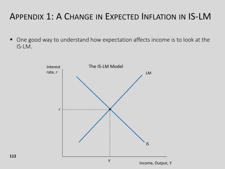
APPENDIX 1: A CHANGE IN EXPECTED INFLATION IN IS-LM
112
One good way to understand how expectation affects income is to look at the IS-LM.
Interest rate, r
Income, Output, Y
IS
The IS-LM Model
LM
r
Y
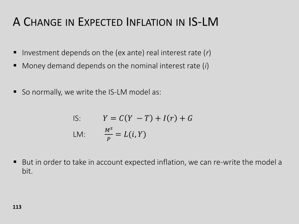
A CHANGE IN EXPECTED INFLATION IN IS-LM
113
Investment depends on the (ex ante) real interest rate (r)
Money demand depends on the nominal interest rate (i)
So normally, we write the IS-LM model as:
IS: 𝑌 = 𝐶 𝑌 − 𝑇 + 𝐼 𝑟 + 𝐺
LM:𝑀𝑠
𝑃= 𝐿(𝑖, 𝑌)
But in order to take in account expected inflation, we can re-write the model a bit.
A CHANGE IN EXPECTED INFLATION IN IS-LM
114
Ex ante real interest rate: 𝑟 = 𝑖 − 𝜋𝑒
So, we can write the IS-LM model as:
IS: 𝑌 = 𝐶 𝑌 − 𝑇 + 𝐼 𝑖 − 𝜋𝑒 + 𝐺
LM:𝑀𝑠
𝑃= 𝐿(𝑖, 𝑌)
Expected inflation then enters as a variable in the IS curve.
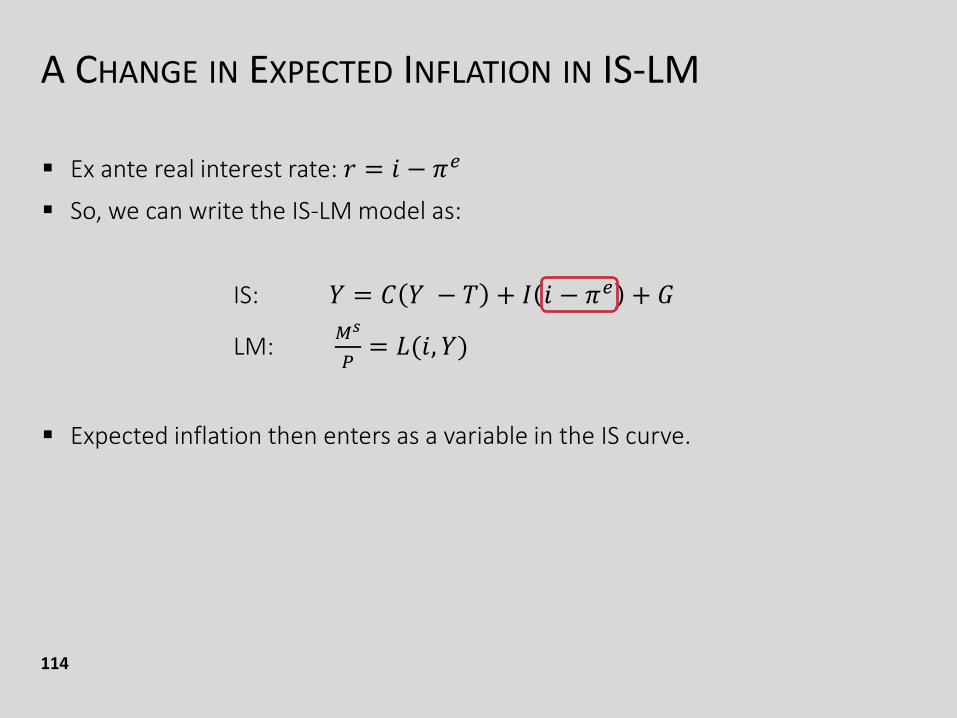
A CHANGE IN EXPECTED INFLATION IN IS-LM
115
Interest rate, i
Income, Output, Y
IS1
LM
Suppose in the initial equilibrium, 𝜋𝑒 = 0, so
r1 = 𝑖1
Now everyone suddenly expects that the price level will fall soon, so
𝜋𝑒 < 0
It raises r for any given i, reducing investment spending, shifting the IS curve.
Both income Y and i drop.But r increases to r2.
r1 = i1
Y1
IS2
𝜋𝑒
i2
Y2
r2
IS: 𝑌 = 𝐶 𝑌 − 𝑇 + 𝐼 𝑖 − 𝜋𝑒 + 𝐺
Reference: Mankiw, G. Macroeconomics, 6e
IS1
A CHANGE IN EXPECTED INFLATION IN IS-LM
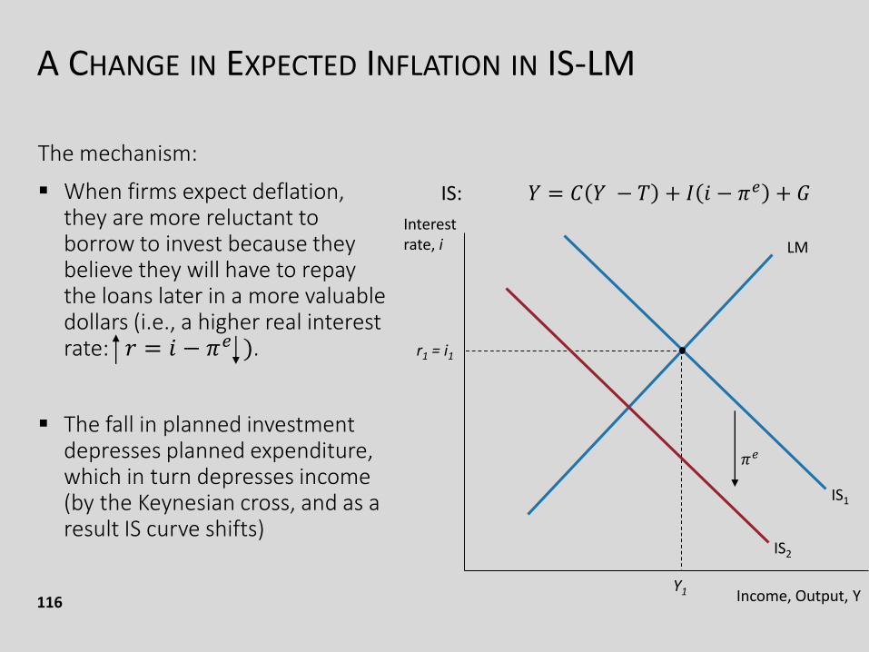
116
The mechanism:
When firms expect deflation, they are more reluctant to borrow to invest because they believe they will have to repay the loans later in a more valuable dollars (i.e., a higher real interest rate: 𝑟 = 𝑖 − 𝜋𝑒 ).
The fall in planned investment depresses planned expenditure, which in turn depresses income (by the Keynesian cross, and as a result IS curve shifts)
LM
r1 = i1
Y1
IS2
𝜋𝑒
IS: 𝑌 = 𝐶 𝑌 − 𝑇 + 𝐼 𝑖 − 𝜋𝑒 + 𝐺
Interest rate, i
Income, Output, Y
IS1
A CHANGE IN EXPECTED INFLATION IN IS-LM
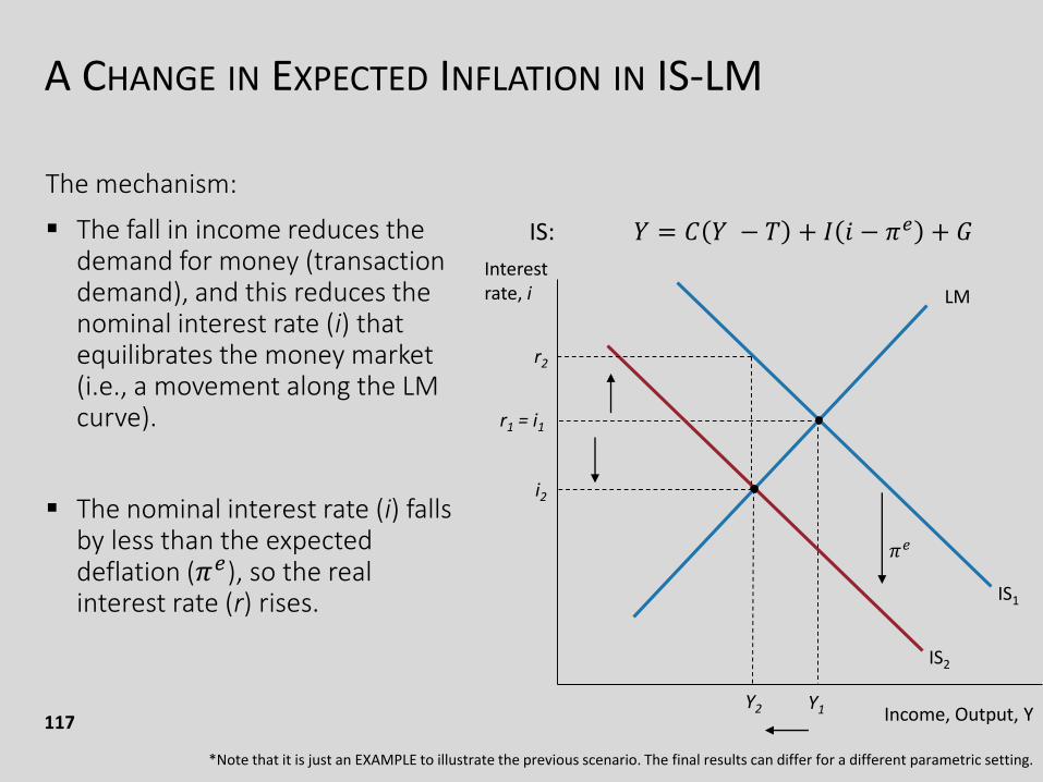
117
The mechanism:
The fall in income reduces the demand for money (transaction demand), and this reduces the nominal interest rate (i) that equilibrates the money market (i.e., a movement along the LM curve).
The nominal interest rate (i) falls by less than the expected deflation (𝜋𝑒), so the real interest rate (r) rises.
LM
r1 = i1
Y1
IS2
𝜋𝑒
i2
Y2
r2
IS: 𝑌 = 𝐶 𝑌 − 𝑇 + 𝐼 𝑖 − 𝜋𝑒 + 𝐺
Interest rate, i
Income, Output, Y
*Note that it is just an EXAMPLE to illustrate the previous scenario. The final results can differ for a different parametric setting.
A CHANGE IN EXPECTED INFLATION IN ADAS
118
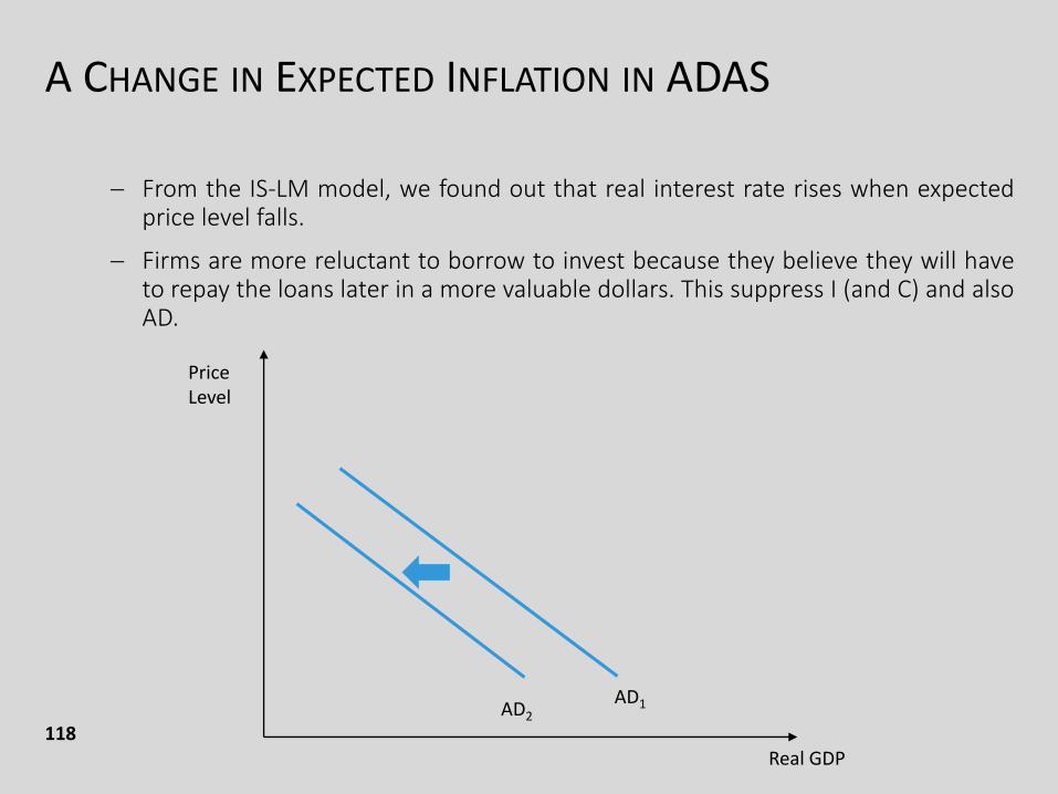
From the IS-LM model, we found out that real interest rate rises when expectedprice level falls.
Firms are more reluctant to borrow to invest because they believe they will haveto repay the loans later in a more valuable dollars. This suppress I (and C) and alsoAD.
Real GDP
Price Level
AD2
AD1
A CHANGE IN EXPECTED INFLATION IN ADAS
119
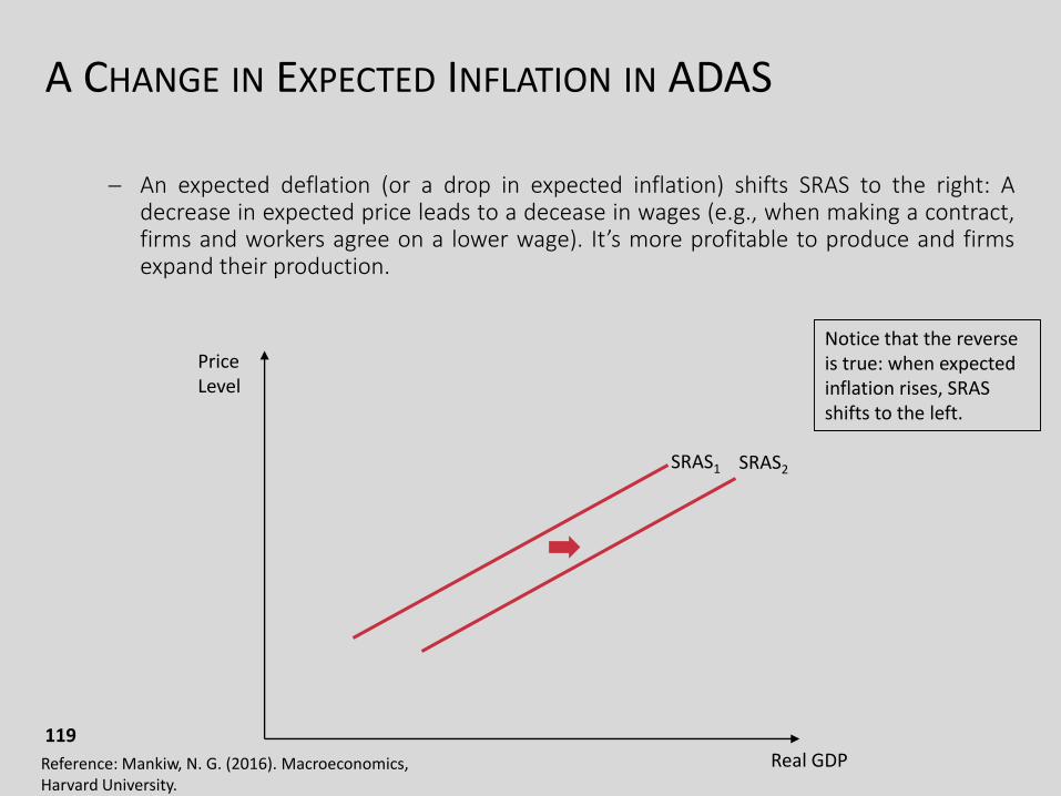
An expected deflation (or a drop in expected inflation) shifts SRAS to the right: Adecrease in expected price leads to a decease in wages (e.g., when making a contract,firms and workers agree on a lower wage). It’s more profitable to produce and firmsexpand their production.
Real GDP
Price Level
SRAS1 SRAS2
Notice that the reverse is true: when expected inflation rises, SRAS shifts to the left.
Reference: Mankiw, N. G. (2016). Macroeconomics, Harvard University.
A CHANGE IN EXPECTED INFLATION IN ADAS
120
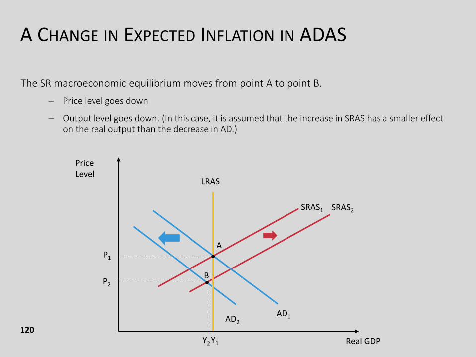
The SR macroeconomic equilibrium moves from point A to point B.
Price level goes down
Output level goes down. (In this case, it is assumed that the increase in SRAS has a smaller effect on the real output than the decrease in AD.)
Real GDP
Price Level
SRAS1 SRAS2
AD2
AD1
•
P1
P2
Y2Y1
LRAS
•
B
A
A CHANGE IN EXPECTED INFLATION IN ADAS
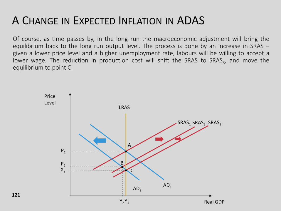
121
Of course, as time passes by, in the long run the macroeconomic adjustment will bring theequilibrium back to the long run output level. The process is done by an increase in SRAS –given a lower price level and a higher unemployment rate, labours will be willing to accept alower wage. The reduction in production cost will shift the SRAS to SRAS3, and move theequilibrium to point C.
Real GDP
Price Level
SRAS1 SRAS2
AD2
AD1
•
P1
P2
Y2Y1
LRAS
•
B
A
SRAS3
• CP3
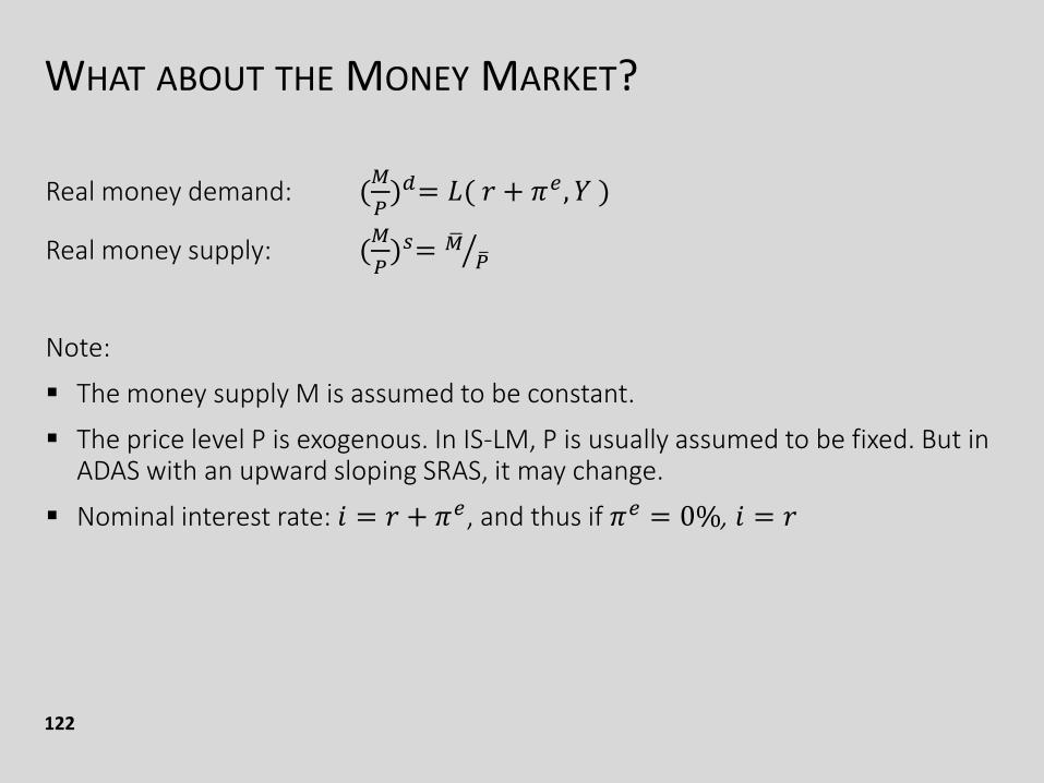
WHAT ABOUT THE MONEY MARKET?
122
Real money demand: (𝑀
𝑃)𝑑= 𝐿( 𝑟 + 𝜋𝑒 , 𝑌 )
Real money supply: (𝑀
𝑃)𝑠= ൗഥ𝑀 ത𝑃
Note:
The money supply M is assumed to be constant.
The price level P is exogenous. In IS-LM, P is usually assumed to be fixed. But in ADAS with an upward sloping SRAS, it may change.
Nominal interest rate: 𝑖 = 𝑟 + 𝜋𝑒, and thus if 𝜋𝑒 = 0%, 𝑖 = 𝑟
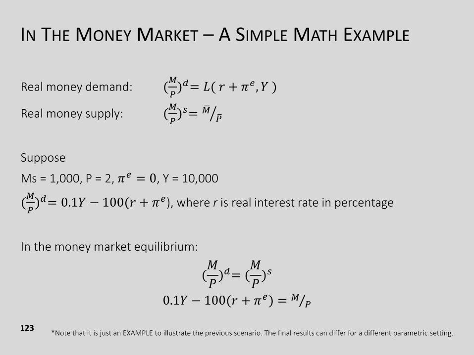
IN THE MONEY MARKET – A SIMPLE MATH EXAMPLE
123
Real money demand: (𝑀
𝑃)𝑑= 𝐿( 𝑟 + 𝜋𝑒 , 𝑌 )
Real money supply: (𝑀
𝑃)𝑠= ൗഥ𝑀 ത𝑃
Suppose
Ms = 1,000, P = 2, 𝜋𝑒 = 0, Y = 10,000
(𝑀
𝑃)𝑑= 0.1𝑌 − 100(𝑟 + 𝜋𝑒), where r is real interest rate in percentage
In the money market equilibrium:
(𝑀
𝑃)𝑑= (
𝑀
𝑃)𝑠
0.1𝑌 − 100(𝑟 + 𝜋𝑒) = Τ𝑀 𝑃
*Note that it is just an EXAMPLE to illustrate the previous scenario. The final results can differ for a different parametric setting.
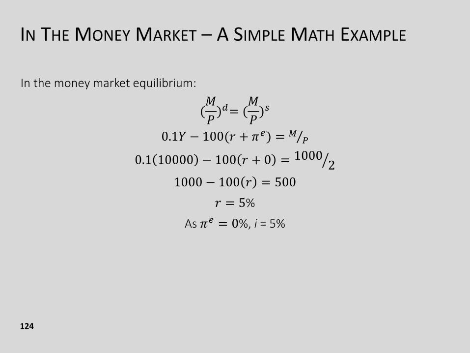
IN THE MONEY MARKET – A SIMPLE MATH EXAMPLE
124
In the money market equilibrium:
(𝑀
𝑃)𝑑= (
𝑀
𝑃)𝑠
0.1𝑌 − 100(𝑟 + 𝜋𝑒) = Τ𝑀 𝑃
0.1 10000 − 100 𝑟 + 0 = ൗ10002
1000 − 100 𝑟 = 500
𝑟 = 5%
As 𝜋𝑒 = 0%, i = 5%
IN THE MONEY MARKET – A SIMPLE MATH EXAMPLE
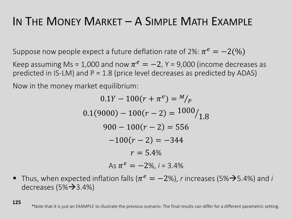
125
Suppose now people expect a future deflation rate of 2%: 𝜋𝑒 = −2(%)
Keep assuming Ms = 1,000 and now 𝜋𝑒 = −2, Y = 9,000 (income decreases as predicted in IS-LM) and P = 1.8 (price level decreases as predicted by ADAS)
Now in the money market equilibrium:
0.1𝑌 − 100(𝑟 + 𝜋𝑒) = Τ𝑀 𝑃
0.1 9000 − 100 𝑟 − 2 = ൗ10001.8
900 − 100 𝑟 − 2 = 556
−100 𝑟 − 2 = −344
𝑟 = 5.4%
As 𝜋𝑒 = −2%, i = 3.4%
Thus, when expected inflation falls (𝜋𝑒 = −2%), r increases (5%5.4%) and idecreases (5%3.4%)
*Note that it is just an EXAMPLE to illustrate the previous scenario. The final results can differ for a different parametric setting.
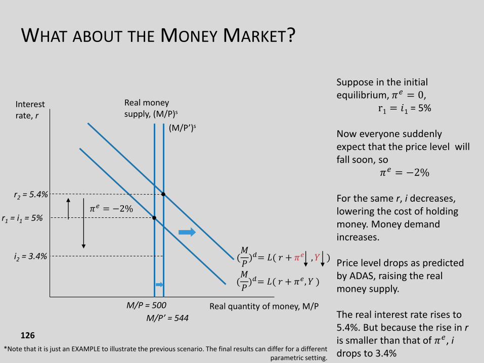
WHAT ABOUT THE MONEY MARKET?
126
Suppose in the initial equilibrium, 𝜋𝑒 = 0,
r1 = 𝑖1 = 5%
Now everyone suddenly expect that the price level will fall soon, so
𝜋𝑒 = −2%
For the same r, i decreases, lowering the cost of holding money. Money demand increases.
Price level drops as predicted by ADAS, raising the real money supply.
The real interest rate rises to 5.4%. But because the rise in ris smaller than that of 𝜋𝑒, idrops to 3.4%
(M/P’)s
Interest rate, r
Real quantity of money, M/P
(𝑀
𝑃)𝑑= 𝐿( 𝑟 + 𝜋𝑒, 𝑌 )
Real money supply, (M/P)s
r1 = i1 = 5%
(𝑀
𝑃)𝑑= 𝐿( 𝑟 + 𝜋𝑒 , 𝑌 )
r2 = 5.4%
i2 = 3.4%
𝜋𝑒 = −2%
M/P = 500
M/P’ = 544
*Note that it is just an EXAMPLE to illustrate the previous scenario. The final results can differ for a different parametric setting.
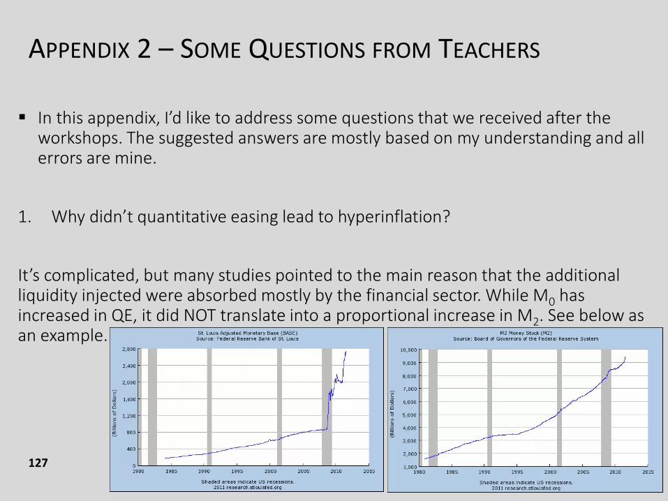
APPENDIX 2 – SOME QUESTIONS FROM TEACHERS
127
In this appendix, I’d like to address some questions that we received after the workshops. The suggested answers are mostly based on my understanding and all errors are mine.
1. Why didn’t quantitative easing lead to hyperinflation?
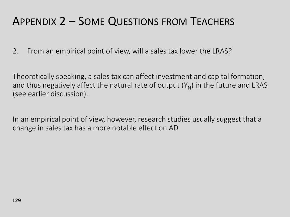
It’s complicated, but many studies pointed to the main reason that the additional liquidity injected were absorbed mostly by the financial sector. While M0 has increased in QE, it did NOT translate into a proportional increase in M2. See below as an example.
APPENDIX 2 – SOME QUESTIONS FROM TEACHERS
128
1. Why didn’t quantitative easing lead to hyperinflation?
The rise in excess reserves of the commercial banks meant that QE did NOT increase M2 as much as we expected.
Ding (2020) also reported that the speed of currency circulation (measured by M2) has been slowing down.
All these mean that there has been a structural change in the money creation process.
https://www.bochk.com/dam/investment/bocecon/SY2020011(en).pdf
APPENDIX 2 – SOME QUESTIONS FROM TEACHERS
129
2. From an empirical point of view, will a sales tax lower the LRAS?
Theoretically speaking, a sales tax can affect investment and capital formation, and thus negatively affect the natural rate of output (YN) in the future and LRAS (see earlier discussion).
In an empirical point of view, however, research studies usually suggest that a change in sales tax has a more notable effect on AD.
APPENDIX 2 – SOME QUESTIONS FROM TEACHERS
130
3. When we use interest rate effect to explain the negative slope of AD, we say ‘an increase in price level raises the nominal money demand, and thus the nominal interest rate’. But what suppresses investment is the real interest rate. Is there any inconsistency?
If the expected inflation is rather constant, which is usually true in SR, the two interest rates move in the same direction. And so, it does not really matter which interest rate to use in the analysis.
APPENDIX 2 – SOME QUESTIONS FROM TEACHERS
131
4. When teaching money demand, some students will argue that factors other than Y and interest rate will also affect money demand. However, these factors sometimes are not considered when it comes to the money demand function. How should we explain this to student?
It is quite a common problem that I come across in teaching, and it does not only apply to money demand. I appreciate that students are thinking deeper instead of taking what’s on the textbook for granted.
It’s often nice to ask the students explain what they have in mind clearly, and discuss with them how these new insights will affect our core analysis (usually it will not). It’s also a good time to explain to students that the core analysis does NOT cover everything, but only the most important and significant impacts. See pp. 16 – 19.
APPENDIX 2 – SOME QUESTIONS FROM TEACHERS
132
5. Is the following correct: Y increases, import increases, net export decreases, AD decreases?
What in the question is correct in some sense (Y increases M, and thus NX will drop), but INCOMPLETE.
Consider an initial increase in AD (e.g. an increase in G) raises Y:
i. An increase in Y then leads to an increase in C, I (induced investment), and M.
ii. An increase in I tends to further raise the AD.
iii. Part of the increase in consumption is likely to be spent on imports. For example, suppose consumption increases by $100, in which $40 is from imports, then there will be a further net increase in AD by $60.
iv. So the final result will be: an increase in Y will lead to a further increase in AD.
This is the multiplier effect.

APPENDIX 2 – SOME QUESTIONS FROM TEACHERS
133
6. The profit tax will affect both the AD and AS. It is difficult for students to determine the overall effect. How can we guide students to analyse?
I would recommend to focus on its impact on AD first. Only after students firmly master the mechanism of how a profit tax affect AD (and thus the macroeconomic equilibrium), should we start introducing the supply-side effects. I usually regard the supply-side effects as ‘adds-on’ of simple ADAS and talk about it in a later stage. There are two reasons:
1) The supply side effects are usually regarded as less important.
2) The demand side effects are more straight-forward and can happen immediately, while the supply side effect takes time to realise (e.g., capital accumulation affect productivity in the long run).
See pp. 32 – 33 for analysis of a profit (corporate) tax on AS.
See pp. 43 – 48 for a complete analysis of such a tax.
APPENDIX 2 – SOME QUESTIONS FROM TEACHERS
134
7. How to explain to students that an economy can produce at a point exceeding the potential output?
The term ‘potential output’ may be misleading – it does NOT refer to the maximum output level of an economy. Rather, it refers to the output level at which the economy’s unemployment rate equals the natural rate of unemployment. Thus, another name for ‘potential output’ is the ‘natural rate of output’ (Okun’s Law describe the relationship between unemployment rate and production).
When the AD is ‘too high’, the economy can be producing at an output greater than the potential output. But note that it is NOT sustainable in the LR.
One easy way for students to understand is to ask them to imagine a situation in which everyone is working overtime – we can certainly produce more than we ordinary do, but it’s a situation that cannot be sustained for long. It’s obviously not a perfect analogy, but a very straight-forward one.
APPENDIX 2 – SOME QUESTIONS FROM TEACHERS
135
8. When a central bank redeems bond, does it mean the central bank issues new note at the same time?
It may not be necessarily true. One can easily imagine a situation that a central bank uses the cash in its own reserve to conduct open market operation (purchasing government bonds).
APPENDIX 2 – SOME QUESTIONS FROM TEACHERS
136
9. When we have a fall in price level, purchasing power of money increases, and thus consumption increases. That is why the output demanded increases, and AD slopes downward.
When there is change in a non price level determinants affecting consumption expenditure, AD changes. In these situations, does the consumption expenditure refer to real consumption expenditure?
We usually put down real output on the X-axis in the ASAD model. And thus, for consistency, all AD components, C, I, G, NX, should be measured in real terms.
APPENDIX 2 – SOME QUESTIONS FROM TEACHERS
137
10. When e-payment is available, we regard there is a decrease in transaction demand for money. But why wouldn't there be an increase in transaction demand for deposits that offsets the decrease in transaction demand for cash, and so holding overall demand for money unchanged?
I think it depends on some behavioural assumptions and which money definition that we use. Let’s consider the widespread use of Octopus card. Intuitively, when Octopus card becomes more popular, people will hold less cash.
Let’s assume
1. People will put the unwanted cash in the bank as saving (but not checking) deposit.
2. People will then maintain a higher deposit balance, but not putting money in financial assets like bonds.
In this case, if we use M1 as the definition of money, money demand decreases.
APPENDIX 2 – SOME QUESTIONS FROM TEACHERS
138
10. When e-payment is available, we regard there is a decrease in transaction demand for money. But why wouldn't there be an increase in transaction demand for deposits that offsets the decrease in transaction demand for cash, and so holding overall demand for money unchanged?
If we use M2 as the definition of money, money demand remains constant (The decline in demand for cash can be offset by an increase in demand for saving deposit).
I do not see a strong reason why assumption 2 above must be true. And if assumption 2 is not true, even if we use M2 as the definition of money, money demand is likely to decrease when Octopus card is more popular.
Reminder: The model in the curriculum assumes a 2-assets model (money:without interest and bond: with interest). When considering the saving deposit(with interest but can perform the transaction demand purpose in reality), theanalysis would become a 3-assets approach.