Embed Size (px)
Citation preview

Learning and Stock Market Participation∗
Juhani Linnainmaa†
The Anderson School at UCLA
November 2005
∗I am truly indebted to Mark Grinblatt for his guidance and encouragement. I also thank Costas Azariadis,Tony Bernardo, Michael Brennan, Stephen Cauley, Christopher Hennessy, Francis Longstaff, Hanno Lustig,Kevin McCardle, Ehud Peleg, Monika Piazzesi, Eduardo Schwartz, Walter Torous, and seminar participantsat the University of California, Los Angeles and Helsinki School of Economics for their comments. I gratefullyacknowledge the financial support from the Allstate Dissertation Fellowship. All errors are mine.
†Correspondence Information: Juhani Linnainmaa, The Anderson School at UCLA,Suite C4.01, 110 Westwood Plaza, CA 90095-1481, tel: (310) 909-4666, fax: (310) 206-5455,http://personal.anderson.ucla.edu/juhani.linnainmaa, email: [email protected].

Learning and Stock Market Participation
Abstract
This paper examines the impact of short-sale constraints on market participation when
agents learn about their investment opportunities. The possibility of binding short-sale
constraints creates a feedback that can keep agents out of the market even if the risk pre-
mium is high. This effect arises with learning because the changes in investment opportu-
nities are correlated with future realized outcomes: an agent will have a poor investment
opportunity set precisely in those future states where her marginal utility is high. Non-
participation arises also in an equilibrium model where agents resolve uncertainty about
the cash-flow covariance between tradable and non-tradable assets. These results suggest
that learning and short-sale constraints can simultaneously generate non-participation, a
sizable risk premium, and insignificant contemporaneous correlation between the stock
return and the income of those who do not participate in the stock market.
1
1 Introduction
Stock market participants have historically been a minority.1 Despite the exceptional historical
equity premium, many individuals stay out of the market. This is a puzzle because everyone
should participate if the risk premium is even slightly positive and there are no frictions or
incomplete markets (Arrow 1965). Many empirical determinants of participation are known.
For example, education matters: 50% of individuals with a college degree own stocks while
this rate is only 20% for those without a degree (Hong, Kubik, and Stein 2004). Wealth is the
strongest determinant of participation: the participation rate increases from 3% to 55% from
the first to the fifth wealth quintile. However, the non-participants are not only those who
have nothing to invest: Mankiw and Zeldes (1991) find that even individuals with more than
$100,000 in liquid assets have a participation rate of only 47.7%. The limited participation
puzzle is our inability to understand why so many individuals choose to stay out of the market.
We propose a novel mechanism that generates non-participation in a perfectly rational
setting. We first describe this mechanism with an example. Suppose an agent works in an
industry sensitive to the macroeconomic conditions. If the economy stays healthy, the agent
retains her job. However, the agent might lose her job in an economic downturn. If this
happens, the agent’s wage covaries positively with the dividends: if the economy recovers,
firms pay higher dividends and the agent is rehired. However, if the economy remains weak,
firms pay low dividends and the agent receives no labor income. The unemployed agent would
hedge against the risk of not finding a new job by shorting the market.
Suppose now that the agent cannot open a margin account in this unemployed state. This
inability to hedge has two consequences. First, the direct effect is that the agent stays out
of the market after losing her job, generating a welfare loss relative to the “hedging allowed”
case. Second, this potential future welfare loss is important at an earlier date for the employed
agent. If the agent invested in the market today, an economic downturn would have important
repercussions: the agent would not only be unemployed and restricted from hedging but she
would also have high marginal utility because she invested. By staying out of the market
today, the agent hedges against this risk.
1Only the latest Survey of Consumer Finances from 2001 finds that, for the first time in the US history,stockholders have become a majority with a 51.9% participation rate. The participation rate was 31.7% in1989. The SCF participation rates include direct and retirement account holdings of stocks and stock mutualfunds.
2

This paper explores this mechanism and its consequences. We first demonstrate this
feedback effect from future portfolio constraints with a stylized life-cycle model where an agent
learns about the risk premium over time. Because the agent learns about the risk premium,
the agent faces poor investment opportunities after bad realizations. (For example, the agent
revises her beliefs downwards after a low realized return.) We show that the agent may stay
out of the market despite a large risk premium.2 We also introduce implied risk-aversion as a
measure of how much learning and portfolio constraints skew investor behavior. For example,
an agent who stays out of the market despite a high risk premium appears infinitely risk-averse
to an outsider who ignores the role of learning.
We then consider an equilibrium model where heterogeneous agents resolve uncertainty
about the covariance between their nonfinancial income and dividends. Specifically, we con-
sider the case where one of the agents becomes unemployed after a low dividend. We use
this model to address two questions. First, does the unemployment risk together with market
incompleteness generate a hedging demand that keeps the agent out of the market at an earlier
date? Second, what are the consequences of this type of non-participation on the size of the
risk premium? The latter question is important because the limited participation puzzle is
intimately connected to the size of the equity premium.3
We demonstrate two results. The first result is that the risk of binding constraints alone
may induce an agent to stay out of the market at date zero: the agent would participate
today if she could hedge in the unemployed state. The second result is that the risk premium
is high relative to the unconstrained economy—i.e., the same economy but without portfolio
constraints—when the agent is currently out of the market, but
1. would buy a positive amount of the asset if the short-sale constraints were lifted and
2. is close to being indifferent between participating and not participating in the future.
2Learning is central to this non-participation mechanism. For example, it would not be surprising to findthat an agent with currently poor investment opportunities stays out of the market. However, our findingis more surprising: the feedback from future trading restrictions can be so strong that an agent reduces herholdings to zero despite a high risk premium.
3For example, Hong, Kubik, and Stein (2004) motivate their analysis by suggesting that an understandingof what drives participation can shed light on the equity premium puzzle of Mehra and Prescott (1985). Yet,most studies that examine why some individuals do not participate sidestep this issue. It is not obvious whatthe effect on the risk premium should be. For example, if the short-sale constraints let the participating agentsto hold only the entire market (instead of holding more), they only need to be compensated with a smaller riskpremium.
3

This risk premium result holds also for agents with log-preferences. Hence, an agent may stay
out at date 0 even though her labor income is constant, her preferences would generally lead
to myopic behavior, and the risk premium is relatively high. This suggests that an empirical
analysis of the determinants of non-participation may be difficult when agents hedge against
the future risks of not being able to trade all the assets as smoothly as classical models presume.
The rest of the paper is organized as follows. The next section discusses related research.
Section 2 solves a tractable life-cycle model that illustrates the feedback mechanism. Section
3 formulates a heterogeneous-agents equilibrium model with non-participation. Section 4
concludes.
1.1 Relation to Prior Research
1.1.1 Parameter Uncertainty and Learning
Many recent studies have examined parameter uncertainty (or ambiguity) and learning.4 For
example, Brennan (1998) assumes that agents learn about the expected return in a Merton
(1969) setup; Xia’s (2001) agents learn about the predictive ability of an observable state
variable; Brennan and Xia (2001) show that uncertainty about dividend growth may contribute
towards an explanation to the equity premium puzzle; Epstein and Miao (2003) solve an
equilibrium model where agents have different prior views about the economy; and Pastor
and Veronesi (2005a, 2005b) show that uncertainty about future profitability may explain
both IPO waves and high Nasdaq valuations in the 1990s.
This paper is closely related to the studies on parameter uncertainty. The life-cycle model
of Section 2 is a discrete-time analogue of the Brennan (1998) model where an agent accounts
for the estimation uncertainty in the expected return. The pivotal difference that generates
our non-participation result is that our agent faces trading frictions.
1.1.2 Labor Income, Illiquidity, and Trading Constraints
Human capital is an important component of individuals’ wealth: labor income accounts
for 75% of consumption (Santos and Veronesi 2005). Many studies have studied the role
4Williams (1977), Detemple (1986), and Gennotte (1986) are early contributions to asset pricing and portfoliochoice under parameter uncertainty. Baron (1974) and McCardle and Winkler (1989) are portfolio choice modelswith learning where agents display risk-preference. Bayesian learning in a portfolio choice setup can be viewedas a particular definition of the Merton (1973) ICAPM state-variable.
4

of human capital in asset pricing, beginning with Mayers (1972). For example, Santos and
Veronesi (2005) let agents derive income from two sources, dividends and wage. Their key
assumption is that the total income (the sum of wages and dividends) grows over time while the
wage share depends on economic conditions. This assumption generates return predictability
and the growth/value effect. Lettau and Ludvigson (2004) examine the link between wealth
(including human capital) and consumption and find that only permanent wealth changes
affect consumer spending. Malloy, Moskowitz, and Vissing-Jørgensen (2005a) find asset pricing
success by using firing/hiring data to measure persistent labor income shocks. These studies
emphasize the potential role of labor income for explaining individuals’ consumption choices
and asset prices. This paper’s equilibrium model is related because we let one agent face
the possibility of an unemployment. The key difference to the extant studies is our focus on
how the possibility of future unemployment and trading frictions generate non-participation
already at earlier periods.
Numerous studies have considered the general effects of asset illiquidity and non-tradability.
For example, Longstaff (2001) shows that an agent who must accumulate or unwind positions
over a period of time can behave as if she faced endogenous borrowing and short-sale con-
straints. Liu, Longstaff, and Pan (2003) show that an agent facing jump risk is less willing to
take levered or short positions. Longstaff (2005) considers a two-asset, heterogeneous agents
model where one of the assets is traded initially but then enters a blackout period. He finds
that this non-tradability can significantly skew agents’ portfolio choices and that liquidity is
an important component of an asset’s equilibrium value. Pastor and Stambaugh (2003) find
empirically that assets more sensitive to liquidity command a premium over low-sensitivity
stocks. The common theme in this literature is that agents endowed with an illiquid asset act
more cautiously than they would if the markets were complete and frictionless. In this paper,
the portfolio constraints and learning skew the agents’ behavior.
1.1.3 The Limited Participation Puzzle
The limited participation puzzle has attracted attention for two reasons. The first line of
research examines why so many individuals choose to stay out of the market despite the
exceptional historical equity premium. For example, Vissing-Jørgensen (2002b) suggests that
the decision to stay out of the market may be optimal for about half of the non-participating
5
individuals even if the fixed costs are relatively modest.5 However, the estimated costs are
too high for the other half for these costs alone to be a reasonable explanation to the limited
participation puzzle. Theoretical studies by Dow and Werlang (1992), Ang, Bekaert, and
Liu (2005), Epstein and Schneider (2005), and Cao, Wang, and Zhang (2005) introduce non-
standard utility functions to generate non-participation. Dow and Werlang (1992) (a static
model), Epstein and Schneider (2005), and Cao, Wang, and Zhang (2005) (dynamic models)
rely on ambiguity aversion. The latter papers are related to the present study because the
agents in the paper learn over time. Ang, Bekaert, and Liu (2005) generate non-participation
by assuming that investors are disappointment averse.
The second line of participation research begins with the idea that investor heterogeneity
may generate a higher theoretical equity premium.6 It is possible that if some investors are
shut out of the market, their consumption processes “contaminate” aggregate consumption
data. This could lead to falsely reject consumption-based asset pricing models. For example,
the agents in Basak and Cuoco (1998) face frictions that shut them out of the market. In
equilibrium, these agents’ consumption processes do not covary with aggregate consumption.
These studies argue that data on stockholders’ consumption alone may fare better in asset
pricing because the non-stockholders do not price the assets. Vissing-Jørgensen (2002a) es-
timates the bond and stock return Euler equations separately for market participants and
non-participants and finds support for this idea. The problem with these studies is that even
if they find success, they do not address the question of why non-stockholders are not pricing
the assets. Cochrane (2005, pp. 61) concludes his survey of the extant literature as follows:
“Must we use microdata? While initially appealing, however, its not clear that
the stockholder/nonstockholder distinction is vital. Are people who hold no stocks
really not “marginal?” The costs of joining the stock market are trivial. . . Thus,
5For example, suppose an individual has only $5,000 in liquid assets. If the annual stock market participationcost—e.g., brokerage fees and information costs—is, say, $50, the risk-return tradeoff from the market may notbe good enough to induce the agent to participate.
6For example, Mankiw (1986) and others suggest that particular type of heterogeneity in individuals’ mar-ginal rate of substitution could result into higher premium but conclude that the agents still come close tocomplete risk-sharing even by trading just one asset in a frictionless market. Constantinides and Duffie (1996,pp. 221) note that these negative results are largely due to the assumption that each agent’s labor incomeshare is a stationary process. The paper shows how to match any historical equity premium with time-additivepower utility and idiosyncratic income risk. Cochrane (2005, pp. 57) cautions that the Constantinides andDuffie solution may still require unreasonable level of variation in each individuals’ consumption growth: “Can
it be true that if aggregate consumption growth is 2%, the typical person you meet either has +73% or −63%consumption growth?”
6

people who do not invest at all choose not to do so in the face of trivial fixed costs.”
This paper addresses Cochrane’s critique: the agents in our model face no transaction costs
but choose to stay out of the market in equilibrium because of the possibility that the short-
sale constraints bind in the future. Our paper also complements earlier studies by simul-
taneously considering both the causes (future learning) and consequences (risk premium) of
non-participation.
2 An Example of the Feedback Effect: A Life-Cycle Model
This section solves a tractable life-cycle model where a short-sale constrained agent learns
about the risk premium over time. We use this model to demonstrate the feedback mechanism
before turning to a more realistic equilibrium model in Section 3. We discuss two features of
this model before detailing our assumptions and solving the model.
First, the agent in our model knows that the true risk premium is constant but is uncertain
about its precise value in the beginning. The agent considers the possibility that the risk
premium may turn out to be negative. If this happens, the asset becomes effectively useless
to the agent because of the short-sale constraints. The assumption that the risk premium can
become negative is a shorthand way of modeling subjective investment opportunity sets. For
example, an agent who faces permanent labor income shocks (e.g., she may be hired, fired,
or tenured) wants to short the market when her wage covaries sufficiently with the market
returns even when the risk premium is restricted to strictly positive values.
Second, the stock price follows a binomial tree with constant up- and down-tick para-
meters. This means that the agent might optimally take a short position in the asset and
that the assumption of short-sale constraints has repercussions. Note that if the return dis-
tribution were unbounded from above, the agent would endogenously refrain from any short
positions.7 (The continuous-time equivalent would be either jump-risk or assets that are not
always tradable.) Note that our assumption is not very restrictive for two reasons. First, a
binomial model converges to a diffusion process as the number of horizons increases and the
length of each period shortens. Second, our emphasis is on what happens when the agent
faces exogenous constraints on top of the endogenous constraints and not on the exact nature
7The agent’s utility function also needs to satisfy the Inada conditions—namely that limW→0 U ′(W ) = ∞.
7

of this additional constraint.
2.1 Setup
We make the following assumptions:
• A single agent lives for T + 1 periods, indexed from 0, . . . , T .
• The agent maximizes power utility over date T wealth,
UT (WT ) =W
1−γT − 1
1 − γ. (1)
• There is a single risky stock and a risk-free asset. These assets are traded each period.
The stock price follows a binomial tree (Cox, Ross, and Rubinstein 1979; Liu and Neis
2002):
St+1 =
St(Rf + u) with probability p
St(Rf − d) with probability 1 − p(2)
where ud > 0 to rule out arbitrage. The risk-free asset returns Rf each period for sure.
• The agent decides how much to invest in the risky asset at the beginning of each period
after observing the previous period’s realized return.
• The agent cannot short the stock, θt ≥ 0, where θt is the number of shares.
• The agent knows all the parameters of the economy precisely except for the probability
p. The agent has a Beta-distributed prior about p and updates her beliefs as a Bayesian
at the beginning of each period.
The wealth dynamics from these assumptions are
Wt = Wt−1(Rf + ft−1ǫ), (3)
where ǫ =
u with probability p
−d with probability 1 − p
ft−1 =θt−1St−1
Wt−1(fraction of wealth in stock).
8

��
��
��
��
��
��1
PP
PP
PP
PP
PP
PPq
Wealth: Wt
Beliefs: (αt, βt)
Wealth: Wt(Rf + ftu)
Beliefs: (αt + 1, βt)
Wealth: Wt(Rf − ftd)
Beliefs: (αt, βt + 1)
Date t Date t + 1
p
1 − p
Figure 1: The Agent’s Wealth and Beliefs in the Binomial Model
The agent’s problem can be broken into two steps: an inference problem in which the agent
updates her estimate of p and an optimization problem in which the agent chooses the optimal
investment given the current wealth and the estimate of p (Gennotte 1986; Brennan and Xia
2001). We consider first the inference problem.
2.2 The Agent’s Inference Problem
The agent has a conjugate prior distribution Beta(α0, β0) about p at date 0. The assumption
about a binomial stock price process and a Beta-distributed prior makes the inference problem
particularly tractable. The date t posterior after observing Nt positive stock price movements
is Beta(α0 + Nt, β0 + t − Nt)-distributed (see, e.g., DeGroot (1970, pp. 160)). The mean and
variance of the posterior distribution are given by
Et(p) =α0 + Nt
α0 + β0 + t, vart(p) =
(α0 + Nt)(β0 + t − Nt)
(α0 + β0 + t)2(α0 + β0 + t + 1). (4)
We let αt ≡ α0 +Nt and βt ≡ β0 + t−Nt to denote the date t belief parameters. The intuition
for updating is simple: the parameters of the Beta-distribution keep track of the number of
the stock price’s up- and downticks. For example, if the agent starts with parameters (1, 2),
the parameters become (2, 2) after an uptick and (1, 3) after a downtick. Figure 1 illustrates
how the agent’s wealth and beliefs evolve in this problem.
2.3 The Agent’s Optimization Problem
We solve the agent’s optimization problem with dynamic programming. The agent receives
utility VT (WT ) =W
1−γT
1−γin the last period. (We assume that γ 6= 1.) We begin with the
9

conjecture that the date t + 1 Bellman equation has the form
Vt+1(Wt+1, (αt+1, βt+1)) =W
1−γt+1
1 − γkt+1(αt+1, βt+1) (5)
and then later show that it satisfies this form. With this conjecture, the date t Bellman
equation solves
Vt(Wt, (αt, βt)) = maxft≥0
{Et [Vt+1(Wt(Rf + ftǫ), (αt+1, βt+1))]}
= maxft≥0
{W
1−γt
1 − γ
[αt
αt + βt(Rf + ftu)1−γkt+1(αt + 1, βt)
+βt
αt + βt(Rf − ftd)1−γkt+1(αt, βt + 1)
]}. (6)
We let kut+1 ≡ kt+1(αt+1, βt) and kd
t+1 ≡ kt+1(αt, βt+1) to simplify the notation. The optimal
investment from the first-order condition is
f∗t =
(αt u kut+1)
1γ − (βt d kd
t+1)1γ
(αt u kut+1)
1γ d + (βt d kd
t+1)1γ u
Rf if αt u kut+1 > βt d kd
t+1
0 otherwise.
(7)
The following proposition gives the functional form of the coefficient kt(αt, βt):
Proposition 1. The coefficient kt(αt, βt) that satisfies the Bellman equation (Eq. 6) is given
recursively by
kt(αt, βt) =
(u + d)1−γ
u d
((αt ku
t+1 u)1γ d + (βt kd
t+1d)1γ u)γ
αt + βtR
1−γf if αt u ku
t+1 > βt d kdt+1
αt kut+1 + βt kd
t+1
αt + βtR
1−γf otherwise
(8)
kT (αT , βT ) = 1. (9)
Proof of Proposition 1. This can be proven by substituting the optimal investment (Eq. 7)
into the Bellman equation (Eq. 6). The functional form of kt(αt, βt) given in the proposition
satisfies the resulting equation.
We note two issues before characterizing the agent’s behavior in the model. First, the
10

optimal investment depends only on current wealth and beliefs and not on the sequence of
outcomes. Second, for comparison and for future reference, we can infer the behavior of
a ‘no parameter uncertainty’ agent from the solution. If the agent knows the parameter
p precisely—or does not update her beliefs over time—the coefficient kt(αt, βt) becomes a
function of time alone. It follows (from Eq. 7) that the date t optimal investment of the ‘no
parameter uncertainty’ agent is
f∗t =
(p u )1γ − ((1 − p) d)
1γ
(p u )1γ d − ((1 − p) d )
1γ u
Rf if p u > (1 − p) d
0 otherwise.
(10)
The agent invests a positive amount if the risk premium is positive. Otherwise the agent
would short the stock.
2.4 Characterizing Optimal Behavior
We now characterize the agent’s optimal behavior in the model. All proofs are in Appendix
A. We begin with the key result that an agent may stay out of the market even when the risk
premium is strictly positive:
Proposition 2. The optimal investment is decreasing in the variance of the prior distribution
if γ > 1 and increasing in the variance if γ < 1.
Corollary 1. ∃ δ > 0 such that an agent with γ > 1 does not invest when E0(ǫ) ≤ δ and an
agent with γ < 1 invests a strictly positive amount when E0(ǫ) ≥ −δ.
These results distinguish our life-cycle model from classical models where an agent invests
a positive amount if the risk premium is positive. A mildly risk-averse agent with γ < 1
prefers uncertainty: the investment is increasing in the variance of the prior. This is the same
as saying that the agent wants to take an actuarially unfair gamble. The agent’s willingness
to pay to learn does not generate this behavior—note that the agent observes realized returns
even without an investment. The reason is that a γ < 1 agent “weights” positive outcomes
more than negative outcomes. Starting from a situation with a negative risk premium, the
agent knows that the risk premium may turn out to be positive. The agent maximizes her
wealth in the states with good investment opportunities by investing today.
11

An agent with γ > 1, on the other hand, needs to be compensated for the extra source of
risk brought on by parameter uncertainty. This generates a non-participation region: faced
with enough uncertainty, an agent with γ > 1 allocates everything in the risk-free asset
even if her prior about the risk premium is strictly positive. This difference to the γ < 1
case arises because this more risk-averse agent weights negative outcomes more than positive
outcomes. Starting from a situation with a positive risk premium, the agent knows that the
risk premium may turn out to be negative. The agent maximizes her wealth in the states with
poor investment opportunities by staying out today.8
It is straightforward to show that if the short-sale constraints are lifted, the agent behaves
similar to the Brennan (1998) agent. The future learning still matters—e.g., an agent with
risk-aversion above γ > 1 always invests proportionally less than what she would invest in
absence of parameter uncertainty—but the investment is always strictly positive if the risk
premium is positive.9 The non-participation result requires that the short-sale constraints
bind in some future states—i.e., that the expected risk premium can turn negative. As noted
earlier, this assumption is a shorthand way of modeling subjective investment opportunity
sets. For example, an agent may invest in an MBA degree and receive labor income out of
this degree for the rest of her life.
The following proposition determines what beliefs an agent who knows “nothing” about
the expected return must have about p to invest in the asset:
Proposition 3. An agent with maximally dispersed prior who faces two periods of investment
(T = 2) invests if and only if
E0(p) ≥1
1 +u
d
(u + d
d
)1−γ. (11)
8The interpretation of differences in weighting is intuitive. From the form of the value function, the solutionto the model is similar identical to the no-learning case except that the agent “weights” different outcomes usingkts as the weights. To see how these weights change, consider the last period of investment (time T − 1). First,if an agent with γ > 1 does not invest, kT−1(αT−1, βT−1) = 1, and if the agent invests, kT−1(αT−1, βT−1) < 1.Hence, the agent weights poor future opportunities more, or put differently, the indirect utility is convex insome regions. Second, if an agent with γ < 1 does not invest, kT−1(αT−1, βT−1) = 1, and if the agent invests,kT−1(αT−1, βT−1) > 1. Hence, the agent weights good future opportunities more—the indirect utility functionis more concave in some regions.
9The non-participation result does not depend on the assumption that there is no intermediate consumption.The solution is nearly identical with time-separable power utility; the distinction is that each period the agentfirst consumes some fraction of her wealth and then allocates the rest between the assets.
12

This proposition assumes that the agent has a completely non-informative prior—i.e.,
the variance of the prior is maximized by fixing E0(p) and letting α, β → 0—and gives the
boundary for the uptick probability that guarantees a positive investment. Note that because
the optimal investment is decreasing in the variance of the prior for γ > 1 -agents, this
proposition gives the upper-bound of what these agents require of E0(p) when their priors
became completely uninformative. We can use this result show that the non-participation
region can be substantial even in a three-period setting. For example, suppose that the risk
premium is symmetric around zero (u = d). Then, while an agent with γ = 2 may require
that the probability of an uptick is E0(p) ≥ 0.67, an agent with γ = 5 may stay out of the
market until E0(p) ≥ 0.94! If u = d = 20%, these boundaries correspond to (expected) risk
premia of 6.7% and 17.6%, respectively.
Suppose that there is an outsider who observes the agent’s behavior, ignores parameter
uncertainty, and backs out what the agent’s behavior implies about her risk-aversion. The
following proposition shows this implied risk-aversion has an intuitive form:
Proposition 4. An outsider who sets p = E0(p) infers the agent’s risk-aversion as being
γ = γ
log
(αu
βu
)
log
(αu
βd
)+ log
(ku
kd
) when αuku > βdk− and αu > βd. (12)
This implied risk-aversion is strictly higher than the true risk-aversion γ if γ > 1 and strictly
less if γ < 1.
This measure quantifies the impact of parameter uncertainty and short-sale restrictions on
portfolio choice. We know from Proposition 2 that an agent with γ > 1 always appears strictly
more risk-averse than she really is to an outsider who ignores parameter uncertainty. At the
limit, an agent who stays out of the market when Et[ǫ] > 0 appears infinitely risk-averse.
2.5 Examples
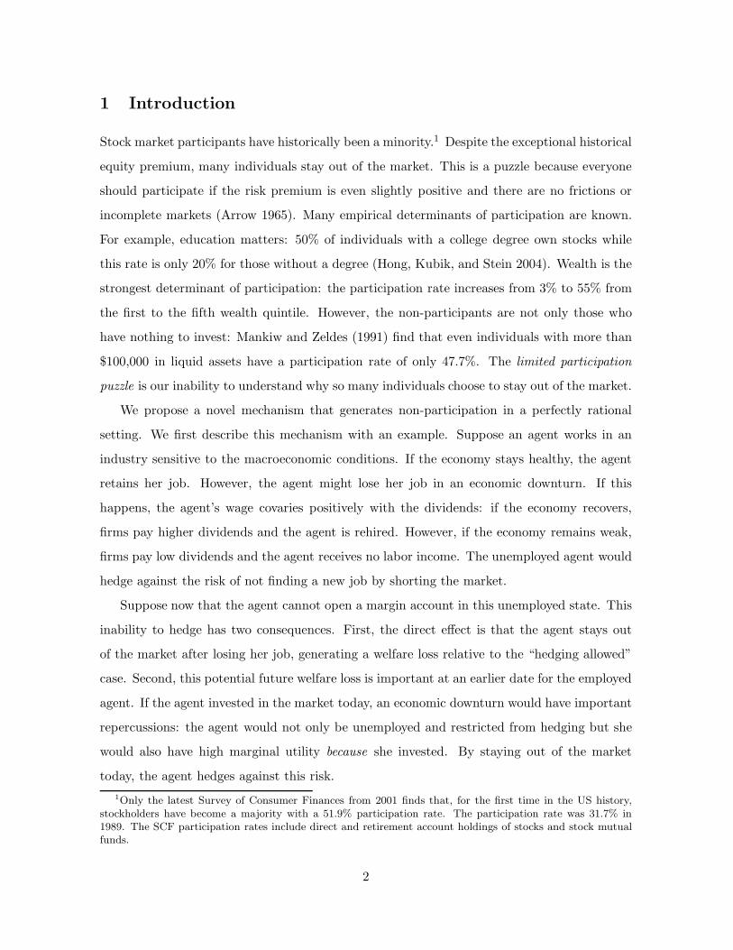
Figure 2 illustrates the results by plotting the optimal investment for an agent with a risk-
aversion of γ = 2 and an investment horizon of T = {10, 50} periods. The optimal investment
is drawn as a function of the parameters of the prior distribution, (α, β). The non-participation
13

0 1 2 3 4 5 6 7 8 9 100
1
2
3
4
5
6
7
8
9
10Panel A: Wealth Invested (γ = 2, T = 10)
α ("number of upticks")
β (
"num
ber
of d
ownt
icks
")
Figure 2: Optimal Investment and Implied Risk-Aversion. An agent with power-utilityover terminal date T wealth trades a risky stock. The stock price follows a binomial process: St+1 =St(Rf + u) with probability p and St+1 = St(Rf − d) with probability 1 − p. The agent has a Beta-distributed prior about p and updates her beliefs as a Bayesian. This figure sets Rf = 1, u = d = 0.2.Panels A and B show optimal investments for an agent with risk-aversion γ = 2 when there are T = 10or T = 50 periods of investment. The optimal investment is drawn as a function of the parameters ofthe prior distribution, (α, β). The 45◦ line is the fair-gamble threshold; i.e., when α = β, the agent’sprior about the excess return is zero. The white area between the diagonal and the filled region isthe non-participation region where the agent does not invest despite a positive risk premium. Panel Cshows the implied risk-aversion for the γ = 2, T = 10 case. The implied risk-aversion (from Eq. 12) isthe solution to an inference problem: how risk-averse does the agent appear to an outsider who ignoresparameter uncertainty. The z-axis is truncated for implied risk-aversions above ten.
region is the white area between the 45◦ line and the filled area. Note that a Merton (1969) or
Brennan (1998) agent would enter the market for all parameters to the right of the diagonal.
In contrast, our agent stays out of the market for a wide range of parameters because of the
risk of binding short-sale constraints.
The figure also plots the implied risk-aversion for the T = 10 period case. The implied
risk-aversion increases sharply when the agent moves towards the non-participation region or
when the variance of the prior increases. Note that the implied risk-aversion is significantly
above the true value of γ = 2 for all parameters in the figure.10 These life-cycle model results
10These plots are for an investor with moderate risk-aversion, γ = 2, and the results are more dramatic formore risk-averse agents. Many studies find relative risk-aversions above two. For example, Nielsen and Vissing-Jørgensen (2005) get an estimate around 5 from data on labor incomes and educational choices; Halek andEisenhauer (2001) obtain a distribution of estimates with a median of 0.89 and a mean of 3.4 with insurancedata; Bliss and Panigirtzoglou (2004) derive (“representative agent”) mean estimates between 2 and 8 from theFTSE100 and S&P 500 option prices; Brennan and Xia (2001) suggest that a relative risk-aversion as high as
14

0 1 2 3 4 5 6 7 8 9 100
1
2
3
4
5
6
7
8
9
10Panel B: Wealth Invested (γ = 2, T = 50)
α ("number of upticks")
β (
"num
ber
of d
ownt
icks
")
02
46
810
0
5
10
2
3
4
5
6
7
8
9
10
α ("number of upticks")
Panel C: Implied Risk−Aversion (γ = 2, T = 10)
β ("number of downticks")
Impl
ied
Ris
k−A
vers
ion
Figure 2: Optimal Investment and Implied Risk-Aversion (cont’d)
show that a short-sale constrained investor with limited information may optimally stay out
of the market even if the (perceived) risk premium is sizable.
We have focused on the possibility that a short-sale constrained agent may stay completely
out of the market because of the feedback from the short-sale constraints. However, more
generally, the possibility of binding constraints always reduces the optimal date 0 portfolio
holdings of a γ > 1 agent. For example, suppose that a γ = 2 agent with an initial wealth of
15 may be reasonable on theoretical grounds.
15
$10,000 is offered two double-or-nothing gambles and that the agent has a prior Beta(0.23, 0.2)
about the probability of winning (E0(p) = 0.535). The optimal date 0 investment is very
sensitive to learning and constraints:
• No learning, no short-sale constraints. The agent takes p = 0.535 as a fixed
parameter and invests $349.
• Learning, no short-sale constraints. The agent invests $289.
• Learning, short-sale constraints. The agent stays out.
If we now fix the mean and decrease the variance of the prior by moving to Beta(0.575, 0.5)-
distribution, the second scenario investment increases to $296 and the optimal investment
under short-sale constraints becomes positive but is still only $162. We now turn to an
equilibrium model that dispenses some of our unrealistic assumptions and shows that the
same non-participation mechanism arises with permanent labor income shocks.
3 An Equilibrium Model with Non-Participation
This section solves an heterogeneous-agents equilibrium model where one of the agents may
lose her job at a later date. The purpose of this model is two-fold. First, we show that
the uncertainty about future labor income can significantly skew today’s decisions when the
agent is restricted from hedging with the risky asset. This generates the same type of non-
participation as observed in Section 2’s life-cycle model: the agent stays out only because
of the risk of binding constraints. Second, we examine what consequences this type of non-
participation has on the risk premium. For example, the first intuition would be that an
introduction of short-sale constraints (if they matter at all) would reduce the risk premium:
because the remaining agents only need to hold the entire market and not more, they require
smaller compensation for risk.11 However, we show that non-participation from the feedback
effect can lead to a higher risk premium.
11For example, Cao, Wang, and Zhang (2005) generate non-participation with ambiguity aversion and findthat the risk premium in the full economy is always higher than what it is in the limited participation economy.
16

3.1 The Economy
We assume the following:
• There are two agents, indexed i ∈ {A,B}, who live for three periods, t = 0, 1, 2. Trading
takes place at dates 0 and 1.
• The agents maximize power utility over date 2 wealth,
U i =W i
21−γ
− 1
1 − γ. (13)
The agents have the same risk-aversion parameter.
• There is a single risky asset in unit net supply. This asset pays a high dividend Dh
with probability p and a low dividend Dl with probability 1− p at dates 1 and 2, where
Dh > Dl.
• A risk-free technology with a gross-return of R is in perfectly elastic supply.
• The agents are initially endowed shares θi and consumption good Xi.
• There are short-sale restrictions on the risky asset, θit ≥ 0, where θi
t is the agent i’s
tradable asset holdings at date t.
• The agents are endowed with a non-tradable asset (e.g., human capital) that pays income
(e.g., wage) at dates 1 and 2. If the date 1 dividend is high, agent i receives a payoff of
yi,h1 at date 1. If the dividend is low, the agent receives y
i,l1 .
• The date 2 income is contingent on the date 1 dividend. If the date 1 dividend is high,
the date 2 income is yi,h2,h or y
i,l2,h and if the dividend is low, the date 2 income is y
i,h2,l or
yi,l2,l.
The last assumption lets agents resolve uncertainty about their future income at date 1. A
natural interpretation for this date 1 signal is the risk of losing a job due to a macroeconomic
shock. The key insight captured by the model is that permanent labor income shocks are pos-
itively correlated with macroeconomic shocks. We assume two states and perfect correlation
17

��
��
��
��
��:
��
��
��
��:
XX
XX
XX
XXz
XX
XX
XX
XX
XXz�
��
��
��
�:
XX
XX
XX
XXz
Date 0 Date 1 Date 2
the agent
is endowedwith θi, X i
Dh, yi,h1
Dl, yi,l1
Dh, yi,h2,h
Dl, yi,l2,h
Dh, yi,h2,l
Dl, yi,l2,l
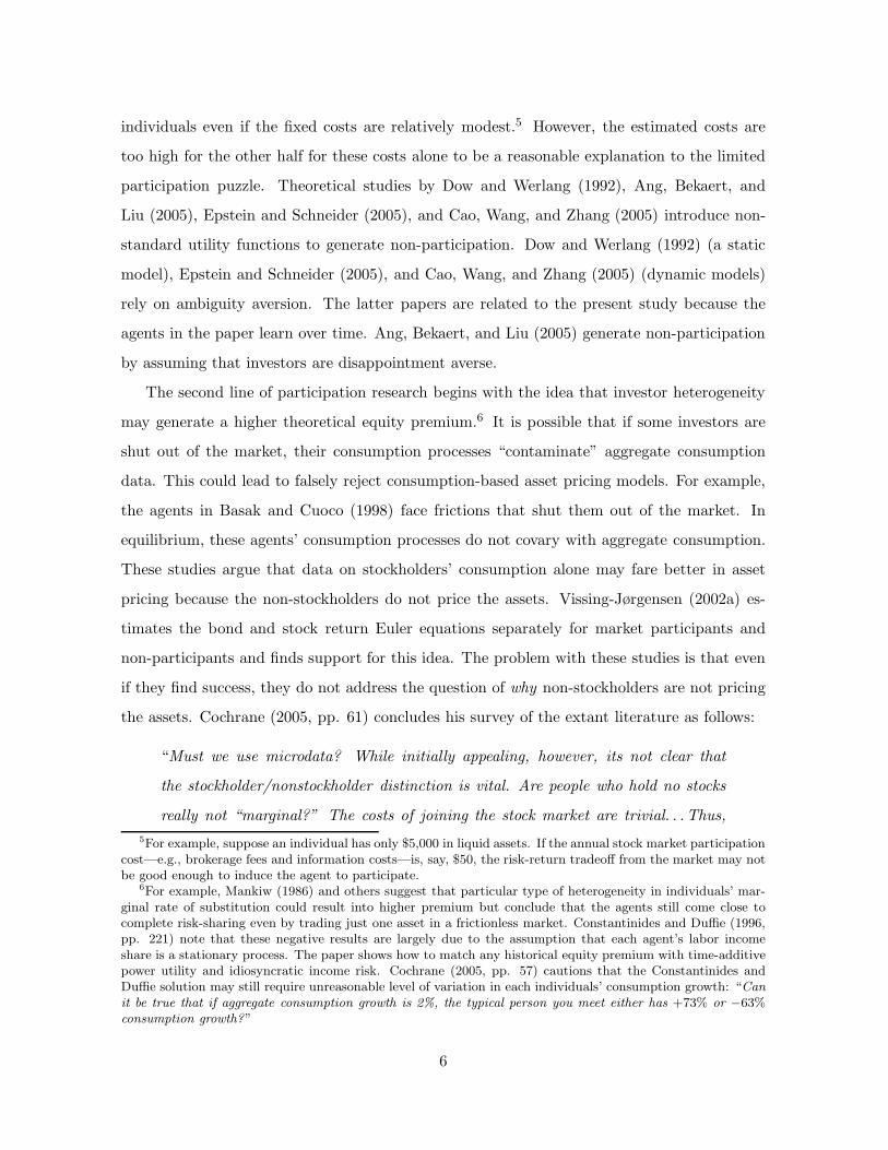
Figure 3: The Timeline for Agent i in the Equilibrium Model
between the assets for tractability.12
Figure 3 shows the timeline of the events for Agent i. The agent starts at date 0 with an
endowment of shares and the consumption good. She decides how much to hold of the risky
asset and puts the rest into the risk-free asset. The agent receives dividend and non-tradable
asset income at date 1. She also learns the values of the date 2 incomes and then makes
the date 1 investment decisions. Finally, the agent receives date 2 payoffs and consumes her
terminal wealth.
We proceed as follows in the remainder of this section. First, we solve the equilibrium
prices in an economy that does not have short-sale constraints. Second, we compute the equi-
librium prices for a particular type of a short-sale constrained economy (“a non-participation
economy”) and give conditions under which these prices constitute equilibrium. Third, we
show that the risk premium in the constrained economy is higher than in an unconstrained
economy (i.e., an otherwise identical economy but without short-sale constraints) in particular
when one of the agents is close to being indifferent between participating and not participating.
3.2 Equilibrium without Short-Sale Constraints
We first solve the date 1 problem and then move backwards to the date 0 problem. Note that
the agent i’s wealth constraints bind with equality:
12The assumption that labor income and dividend streams are perfectly correlated is a very particular as-sumption. This does, however, capture the idea that labor income shocks are affected by market conditions:when an agent’s labor income stream covaries positively with the dividends, the agent is effectively alreadyinvested in the market by default, creating a hedging demand.
18

Date 0: θiP0 + Xi = θi0P0 + Xi
0
Date 1: θi0(P1 + D1) + Xi
0R + yi1 = θi
1P1 + Xi1
Date 2: θi1D2 + Xi
1R + yi2 = W i
2
where Xit is the amount borrowed or lent at the rate R. After substituting out Xi
t , we have
W i2 = W i
1R + θi1(D2 − P1R) + yi
2, (14)
where W i1 ≡ (Xi + θiP0)R + θi
0(P1 + D1 − P0R) + yi1.
3.2.1 Date 1 Decisions and Prices
Agent i’s date 1 Bellman equation in state s = {h, l} solves
V i1,s(W
i1) = max
θ1
E1
(W i
1R + θi1(D2 − P1R) + yi
2,s
)1−γ
1 − γ
. (15)
The optimal demand from the first-order condition is13
θi∗1 (W i
1) =[p(Dh − P s
1 R)]−1γ (W i
1,sR + yi,h2,s) − [(1 − p)(P s
1 R − Dl)]− 1
γ (W i1,sR + y
i,l2,s)
[p(Dh − P s1 R)]−
1γ (Dh − P s
1 R) + [(1 − p)(P s1 R − Dl)]
− 1γ (P s
1 R − Dl). (16)
The date 2 equilibrium price results from summing the agents’ first order conditions and using
the market-clearing condition,∑
i θi =
∑i θ
i0 =
∑i θi
1 = 1:
P s∗1 =
1
R
p(ωh1,s)
−γDh + (1 − p)(ωl1,s)
−γDl
p(ωh1,s)
−γ + (1 − p)(ωl1,s)
−γ, (17)
where ωs′
1,s ≡ R2∑
i
Xi + R
(
D1 +∑
i
yi1,s
)
+∑
i
yi,s′
2,s + Ds′ .
The price is a weighted average of date 2 dividends where the weights are functions of total
wealth in the two states and their probabilities. The initial distribution of allocations does not
matter because both agents’ non-tradable asset income is perfectly correlated with dividends:
the agents can use the tradable asset to hedge perfectly against the income risk.
13Substituting the optimal demand back into Eq. 15, the value function becomes V i1,s(W
i1) =
[(Dh−Dl)Wi1,s+ci,s]1−γ
1−γks. (See Eq. 18 for ci,s and ks.)
19

3.2.2 Date 0 Decisions and Price
Agent i’s date 0 Bellman equation solves
V i0 (Xi, θi) = max
θ0
E0
((Dh − Dl)[(X
i + θiP0)R2 + θ0(P1 + D1 − P0R)R + yiR] + ci
)1−γ
1 − γk
,
where ci,s ≡ yi,h2,s(P
s1 R − Dl) + y
i,l2,s(Dh − P s
1 R),
ks ≡(p
1γ (P s
1 R − Dl)1− 1
γ + (1 − p)1γ (Dh − P s
1 R)1− 1
γ
)γ
. (18)
The optimal demands can be solved from the first-order conditions. The date 0 equilibrium
price follows from summing the agents’ first order conditions and using the market-clearing
condition:
P ∗0 =
1
R
pkhω−γ0,h(P h
1 + Dh) + (1 − p)klω−γ0,l (P l
1 + Dl)
pkhω−γ0,h + (1 − p)klω
−γ0,l
, (19)
where ω0,s = (Dh − Dl)
(
R2∑
i
Xi + R(P s1 + Ds +
∑
i
yi1,s)
)
+∑
i
ci,s.
The equilibrium price is a weighted average of date 1 dividends and the prices in the two states.
The weights are functions of total date 1 wealth in the two states and their probabilities. The
following proposition summarizes these results:
Proposition 5. The equilibrium prices in the unconstrained economy are given by Eqs. 17
(the date 1 prices) and 19 (the date 0 price).
Note that the prices in the unconstrained economy do not depend on how the initial
allocation is distributed between the two agents because the markets are effectively complete.
Hence, the prices in the economy would be the same if there was only a representative agent
who received all the endowments.
3.3 Equilibrium with Short-Sale Constraints
The non-tradable asset income in the economy can generate negative asset demands. For
example, suppose that Agent A’s income covaries positively with dividends after a low date 1
dividend but that Agent B’s income is constant. Agent A would then short the asset after a
20

low dividend if the covariance were sufficiently high. The introduction of short-sale constraints
has two effects. First, the direct consequence is that Agent A increases her date 1 holdings
after a low date 1 dividend from negative to nothing. Second, the restriction on the agent’s
ability to hedge at date 1 may induce Agent A to reduce her date 0 holdings. This effect may
be significant enough to let Agent B hold the whole supply while Agent A exits the market.
We now construct this equilibrium.
3.3.1 Equilibrium Prices in a Non-Participation Economy
The equilibrium prices cannot, in general, be solved in closed-form when there are short-sale
constraints.14 We focus on an exception where Agent A (1) has no initial endowment of the
tradable asset, (2) optimally decides not to hold any asset at date 0 or at date 1 after a low
dividend, and (3) has a holding between 0 and 1 at date 1 after a high dividend. (We later
give the conditions to verify the optimality.) We also add the following assumptions for the
sake of tractability:
1. The risk-free asset yields R = 1.
2. Agent A receives non-tradable asset income only at date 2.
3. Agent B does not receive non-tradable asset income.
4. The agents are not endowed any consumption good, XA = XB = 0.
(Henceforth, we omit agent and date identifiers from y because there is no ambiguity; we
write Agent B’s date 2 income as ys′
s for s, s′ ∈ {h, l}.) The following pricing formulas follow
directly from Proposition 5.
Corollary 2. Non-participation equilibrium is equilibrium where Agent A has zero demand
for the risky asset at date 0 and at date 1 after a low dividend. Both agents have strictly
14The difficulty is that if the date 1 constraints bind for one agent (i.e., the marginal utility at zero holdingsis negative), the market-clearing conditions together with the first-order conditions for the remaining agentsare not (generally) enough to solve for equilibrium prices.
21

positive demands at date 1 after a high dividend. The non-participation equilibrium prices are
P h1 =
p(2Dh + yhh)−γDh + (1 − p)(Dh + Dl + yl
h)−γDl
p(2Dh + yhh)−γ + (1 − p)(Dh + Dl + yl
h)−γ, (20)
P l1 =
p(Dh + Dl)−γDh + (1 − p)(2Dl)
−γDl
p(Dh + Dl)−γ + (1 − p)(2Dl)−γ, (21)
P0 =pkh(P h
1 + Dh)1−γ + (1 − p)kl(P l1 + Dl)
1−γ
pkh(P h1 + Dh)−γ + (1 − p)kl(P l
1 + Dl)−γ, (22)
where ks =(p
1γ (Dh − P s
1 )1γ−1 + (1 − p)
1γ (P s
1 − Dl)1γ−1)γ
.
Note that the equilibrium price after a high dividend is the same as it is in the uncon-
strained economy. Also, the distribution of Agent A’s non-tradable asset income after a low
dividend does not affect any of the prices. We now give the conditions on {yll , yh
l , ylh, yh
h}
that guarantee that the prices in Eqs. 20, 21, and 22 constitute equilibrium. We also show
that there is such an equilibrium. The proof is in the appendix.
Proposition 6. The prices in Corollary 2 are the market-clearing prices if
• Conditions 1A and 1B (Agent A’s optimal holding between zero and one after a high
date 1 dividend):yh
h
ylh
≤ 2Dh
Dh+Dl, (1A)
ylh − yh
h ≤ Dh − Dl. (1B)(23)
• Condition 2 (Agent A’s optimal holding zero after a low date 1 dividend):
yhl
yll
≥Dh + Dl
2Dl. (24)
• Condition 3 (Agent A’s optimal holding zero at date 0):
[p(2Dh + yh
h)−γyhh + (1 − p)(Dh + Dl + yl
h)−γylh
p(2Dh + yhh)−γ2Dh + (1 − p)(Dh + Dl + yl
h)−γ(Dh + Dl)
]−γ
≤p(yh
l )−γ + (1 − p)(yll)−γ
p(Dh + Dl)−γ + (1 − p)(2Dl)−γ. (25)
This system of inequalities has multiple solutions {yhh, yl
h, yhl , yl
l} for any Dh > Dl.
22

Conditions 1A, 1B, and 2 are intuitive. Conditions 1A and 1B state that Agent A’s income
cannot have a too high or too low cash-flow covariance with the tradable asset after a high
date 1 dividend. Otherwise, the agent would want to short or hold more than the entire supply
of the asset, respectively. Condition 2 gives the boundary for the ratio of Agent A’s income
after a low dividend that ensures that the agent does not want to hold any of the asset—note
that this condition mirrors Condition 1A.15
The expression in Condition 3 is less obvious. It states that Agent A must derive higher
expected utility from staying out of the market than from buying an infinitesimal amount
of the asset at the equilibrium price. Note that the LHS of Condition 3 is decreasing in yhh
and ylh and the RHS is decreasing in yh
l and yll . Hence, this condition says that the date 2
income following a low date 1 dividend must be small relative to the high-state income. If an
agent’s income is low after a low dividend, an agent ending up in this state has high marginal
utility. Hence, the intuition for the condition is that the marginal utility in the upstate must
be sufficiently lower than the marginal utility in the downstate. If this is the case, the agent
wants to hedge against the risk of ending up in the downstate by staying out of the market at
date 0. (Note that Condition 3 is always satisfied for sufficiently small yhl and yl
l . In addition,
agents with log-preferences can meet all the conditions. The reason why these agents do not
behave myopically is that the date 1 market incompleteness creates a kink in these agents’
indirect utilities.16)
3.3.2 Example
Figure 4 shows feasible parameters for the non-tradable asset income after a low date 1 divi-
dend, {yhl , yl
l}, that generate non-participation equilibria. The figure assumes that both agents
have log-preferences and that Agent A receives constant income after a high date 1 dividend.
(See the figure text for the parameters of the example economy.) The x-axis is the value of
15Note that there is a minor openness consideration with Conditions 1A, 1B, and 2 in Proposition 6. Theseconditions must be satisfied with strict inequality for equilibrium to hold for sure. Note that if this is not thecase—i.e., if one of the agents is indifferent between participating and not—the agent is precisely at the kinkof her indirect utility function at date 1. Then, the date 0 zero analysis of how an infinitesimal increase in thedate 0 holdings affects the agent’s utility is invalid. We write these conditions with non-strict inequality toremind that the equalities denote the agents’ indifference points.
16In related research, Cochrane, Longstaff, and Santa-Clara (2005) and Longstaff (2005) analyze “Two Lucas(1978) Trees” models and show that market-clearing and black-out (i.e., non-tradability) periods also causelog-utility investors to behave non-myopically.
23

0 0.01 0.02 0.03 0.04 0.05 0.06 0.07 0.08 0.09 0.10
0.05
0.1
0.15
0.2
0.25
0.3
0.35
0.4
0.45
0.5
yll
y lh
θ0U ≥ 0
θ0U < 0
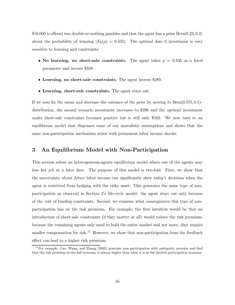
Figure 4: Non-Participation Equilibrium. This figure shows feasible parameters for non-tradable asset income {yh
l , yll} that generate the non-participation equilibrium of Proposition 2. The
following parameters are fixed: Dh = 1.1, Dl = 1, γ = 1, p = 0.5, yhh = yl
h = 0.1 (i.e., the agentshave log-preferences). The x-axis is the low-state income after a low date 1 dividend, yl
l . The y-axis isthe high-state income after a low date 1 dividend, yh
l . The colored grid indicates the set of parametersthat generate the non-participation economy. This region is divided into two sections to indicate whattype of a position Agent A would take in an unconstrained economy. The darker region denotes caseswhere an unconstrained Agent A takes a short position in the risky asset at date 0. The lighter regiondenotes parameters where an unconstrained Agent A takes a long position in the risky asset at date 0.
low-state income and y-axis is the value of the high-state income. Note that the cash-flow co-
variance between Agent A’s non-tradable asset and the tradable asset is positive when yhl > yl
l ;
hence, by keeping the x-axis value fixed and increasing the value on the y-axis, the tradable
asset becomes increasingly worse to the agent.17
The non-participation equilibrium is divided into two areas to indicate what type of date
0 position Agent A would take in an unconstrained economy (i.e., an otherwise identical
economy but without short-sale constraints). The darker area represents cases where Agent
A takes a short position at date 0 in the unconstrained economy. The lighter area consists
of more interesting equilibria where Agent A’s strictly positive date zero holding disappears
when the trading constraints are introduced. Here, the agent would take a long position if it
17Note that the y-axis in the figure is truncated at 0.5—the set of equilibria continues beyond the boundariesof the figure.
24

were not for the possibility of binding short-sale constraints.18
3.4 Risk Premium in the Non-Participation Economy
We now discuss how the date 0 risk premium changes when we move from the unconstrained
economy to the short-sale constrained economy. The proof of the following proposition is in
the appendix:
Proposition 7. The expected date 0 payoff is always higher in the constrained economy than
in an otherwise identical economy but without short-sale constraints (“the unconstrained econ-
omy”). The risk premium is higher in the constrained economy when
1. Agent A is close to participating at date 1 after a low dividend (yh
l
yll
≈ Dh+Dl
2Dl; see Con-
dition 2 of Proposition 6)
2. and Agent A’s date 2 nonfinancial income in the upstate is small relative to the dividends
(yhh, yl
h ≪ Dh,Dl).
These are sufficient conditions.
The second part of the proposition gives sufficient conditions for the date 0 price to be
strictly lower in the constrained economy. Because the expected payoff in the constrained
economy is always higher than the expected payoff in the unconstrained economy, less strict
conditions in practice guarantee that the difference in risk premia between the constrained
and unconstrained economies is positive. The necessary condition is that the date 0 price
cannot change too much in response to the introduction of constraints to reverse the effect of
the higher expected payoff.
However, these stricter conditions have an interesting and important implication: the
risk premium in the constrained economy is particularly high (relative to the unconstrained
economy) when it is most puzzling that Agent A stays out—i.e., when Agent A is indifferent
18Agent A takes a long position at date 0 in the unconstrained economy if
p(2Dh + yhh)1−γ + (1 − p)(Dh + Dl + yl
h)1−γ
p(2Dh + yhh)−γ(2Dh) + (1 − p)(Dh + Dl + yl
h)−γ(Dh + Dl)
≤p(Dh + Dl + yh
l )1−γ + (1 − p)(2Dl + yll)
1−γ
p(Dh + Dl + yhl )−γ(Dh + Dl) + (1 − p)(2Dl + yl
l)−γ(2Dl)
. (Condition 3′) (26)
25
00.02
0.040.06
0.080.1
00.1
0.20.3
0.40.5−6
−4
−2
0
2
4
6
8
10
x 10−4
yll
ylh
r cons
te
− r
unco
nst
e
rconste − r
unconste ≥ 0
rconste − r
unconste < 0
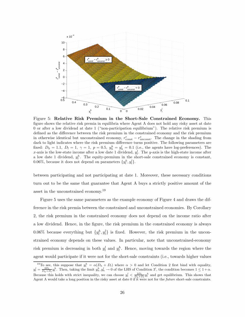
Figure 5: Relative Risk Premium in the Short-Sale Constrained Economy. Thisfigure shows the relative risk premia in equilibria where Agent A does not hold any risky asset at date0 or after a low dividend at date 1 (“non-participation equilibrium”). The relative risk premium isdefined as the difference between the risk premium in the constrained economy and the risk premiumin otherwise identical but unconstrained economy, re
const − reunconst. The change in the shading from
dark to light indicates where the risk premium difference turns positive. The following parameters arefixed: Dh = 1.1, Dl = 1, γ = 1, p = 0.5, yh
h = ylh = 0.1 (i.e., the agents have log-preferences). The
x-axis is the low-state income after a low date 1 dividend, yll . The y-axis is the high-state income after
a low date 1 dividend, yhl . The equity-premium in the short-sale constrained economy is constant,
0.06%, because it does not depend on parameters {yhl , yl
l}.
between participating and not participating at date 1. Moreover, these necessary conditions
turn out to be the same that guarantee that Agent A buys a strictly positive amount of the
asset in the unconstrained economy.19
Figure 5 uses the same parameters as the example economy of Figure 4 and draws the dif-
ference in the risk premia between the constrained and unconstrained economies. By Corollary
2, the risk premium in the constrained economy does not depend on the income ratio after
a low dividend. Hence, in the figure, the risk premium in the constrained economy is always
0.06% because everything but {yhl , yl
l} is fixed. However, the risk premium in the uncon-
strained economy depends on these values. In particular, note that unconstrained-economy
risk premium is decreasing in both yll and yh
l . Hence, moving towards the region where the
agent would participate if it were not for the short-sale constraints (i.e., towards higher values
19To see, this suppose that yhl = α(Dh + Dl) where α > 0 and let Condition 2 first bind with equality,
yll = 2Dl
Dh+Dlyh
l . Then, taking the limit yhh, yl
h → 0 of the LHS of Condition 3′, the condition becomes 1 ≤ 1+α.
Because this holds with strict inequality, we can choose yll <
2Dl
Dh+Dlyh
l and get equilibrium. This shows thatAgent A would take a long position in the risky asset at date 0 if it were not for the future short-sale constraints.
26

of yhl ), the risk premium increases. Note that in this case the area with positive (relative)
risk premium almost coincides with the “positive unconstrained investment”-area in Figure
4. Although this does not always need to be the case, Proposition 7 ensures that if we move
far enough into the correct direction without breaking equilibrium, the risk premium spread
is eventually positive.
3.5 Implications of the Model
Our model generates non-participation by assuming that individuals may face binding trading
restrictions in the future. A natural interpretation for the date 1 signal is the risk of losing
a job due to a macroeconomic shock. Poor economic growth induces firms to cut workforce
and dividends. If an agent loses her job because of an economic downturn (i.e., a low date
1 dividend), she faces a positive covariance between her wage and dividends; a subsequent
turnaround in the economy makes it more probably that the agent is hired and dividends
increase. However, a further weakness in the economy means that dividends stay low and the
agent is likely to remain jobless. In this context, the short-sale constraint assumption states
that the jobless agent at date 1 finds it impossible to open a margin account and short the
market to hedge against the risk of not finding a new job. If there is no initial downturn at
date 1 (i.e., a high date 1 dividend), the agent retains her job.20
There is empirical support to the idea that learning about labor income (and not just the
contemporaneous covariance with the stock market) may affect market participation and asset
prices. First, Malloy, Moskowitz, and Vissing-Jørgensen (2005b) find that stockholders’ (i.e.,
excluding non-participants) long-run consumption risk does particularly well in pricing asset
returns. Malloy, Moskowitz, and Vissing-Jørgensen (2005a) find asset pricing success by using
firing/hiring data to measure persistent labor income shocks, consistent with our interpretation
of the model’s date 1 signal. Second, Guvenen (2005) considers a model where individuals enter
the labor market with a prior belief about their income profiles and estimates that individuals
can forecast (only) 40 percent of variation in income rates at time zero. This suggests that
uncertainty about future labor income is a very real source of risk to most individuals. Finally,
20An alternative set of assumptions that generate same type of prediction involves the housing market. Thehousing market is illiquid and positively correlated with the stock market. The extant research has recognizedthe importance of homeownership on asset allocation (Cauley, Pavlov, and Schwartz 2005; Yao and Zhang2005). Homeownership acts in the same way as human capital in the context of our model. An agent may notwant to invest in the stock market because the home is already effectively such an investment.
27

Vissing-Jørgensen (2002b) finds that a higher volatility of nonfinancial income has a negative
impact on the probability of market participation. This is consistent with our model where it is
the uncertainty about future labor income, not the current covariance between labor income
and stock returns that generates non-participation. For example, in our non-participation
equilibrium, the date 0 one-period correlation between labor income and the asset return is
trivially zero.
The most interesting feature of our model is not that it generates non-participation but
what it implies about the risk-sharing and risk premium in the economy. The standard
motivation for the limited participation puzzle is the question why many individuals choose to
stay out despite very high historical equity premium. An implication of our model is that the
risk premium is relatively high in the constrained economy precisely when it is most puzzling
that some agents decide to stay out. For example, an agent with log-preferences would take a
long position in the risky asset if it were not for the risk of facing binding constraints in the
future. The practical implication of this result is important: an econometrician who ignores
uncertainty, frictions, and the permanent shocks to investors’ investment opportunities may
encounter difficulties in explaining not only limited participation but also the risk premium.
4 Conclusions
This paper describes an intuitive mechanism that keeps some individuals out of the market
even when there are no participation costs and when the current equity premium is high:
uncertainty about investment opportunities and learning together with the possibility of bind-
ing trading restrictions. The life-cycle model illustrates this mechanism. Suppose that an
agent has a prior about the risk premium and revises her beliefs after each new observation.
A consequence of this setup is that the future changes in investment opportunities are posi-
tively correlated with realized returns. (For example, the agent revises her beliefs downwards
after observing a low return.) Thus, a short-sale constrained agent is unable to profit from
her refined information in those future states where she has learned that her investment op-
portunities are poor. Moreover, because of the positive correlation between realizations and
expectations, these states are precisely the ones where the agent’s marginal utility is high.
This creates a feedback to date zero decisions: because the agent knows that the constraints
28

may become binding in the future, she requires a higher risk premium at date 0.
We generalize this idea with an equilibrium model where agents resolve uncertainty about
the covariance between a non-tradable asset (“human capital”) and a risky asset (“stock”).
This setup creates a similar feedback from future short-sale constraints: the possibility of being
constrained in the future may be enough to induce the agent to leave the market at date 0.
This feedback can thus create situation where the equity premium is high yet an agent with
no nonfinancial income risk today stays out of the market. Our model has the interesting
implication that the equity premium is relatively high precisely when it is most puzzling that
some agents choose to stay out—i.e., when the agent is currently out of the market, but
1. would buy a positive amount of the asset if the short-sale constraints were lifted and
2. is close to being indifferent between participating and not participating in the future.
The result that agents may stay out of the market because of uninsurable shocks in the fu-
ture is potentially important in explaining some negative results in the participation literature.
In our model, the risk of a high covariance generates non-participation. The forward-looking
expectation effect—i.e., agents stay out of the market before their labor income covaries posi-
tively with the market—may make it difficult to detect the role of labor income in microdata.
For example, our model’s mechanism can explain why Vissing-Jørgensen (2002b, pp. 33)
concludes:
“. . . the consumption growth of non-stockholders covaries substantially less with
the stock return than the consumption growth of stockholders. . .This indicates that
the primary reason for nonparticipation is not that nonstockholders are faced with
nonfinancial income which is highly correlated with stock market returns.”
Our results suggest that learning and labor income shocks driven by macroeconomic conditions
may simultaneously generate non-participation, a sizable equity premium, and an insignificant
contemporaneous correlation between the stock return and the income of those who do not
participate.
29

A Proofs
We first prove Propositions 2, 3, and 4 for the case when T = 2 and when βd−u < αu < (β+1)d
holds for the prior distribution.21 (We omit subscripts; e.g., α denotes α0.) Eq. 7 shows that
under this assumption learning matters: the agent invests at time 1 only if the date 0 outcome
is positive. (If αu < βd − u, the agent never invests at date 0; if αu > (β + 1)d, the agent
always invests at date 0. Propositions 2 and 4 also hold for the latter case.)
The optimal date 0 investment (if any) in this case is
f∗0 =
(αu)1γ (u + d)
1γ−1(((α + 1)u)
1γ d + (βd)
1γ u)− (βd)
1γ (ud)
1γ (α + β + 1)
1γ
(αu)1γ (u + d)
1γ−1(((α + 1)u)
1γ d + (βd)
1γ u)
d − (βd)1γ (ud)
1γ (α + β + 1)
1γ u
Rf
=α
1γ (u + d)
1γ−1(((α + 1)u)
1γ d + (βd)
1γ u)− (rd)
1γ (ud)
1γ (α + β + 1)
1γ
u1γ (u + d)
1γ−1(((α + 1)u)
1γ d + (βd)
1γ u)
d − (rd)1γ (ud)
1γ (α + β + 1)
1γ u
Rf (27)
where we use Eq. 7 and Proposition 1. We define r = βα
in the second line. With this
substitution, the variance of the prior is decreasing in α while the mean stays constant.22
Proofs of Proposition 2 and Corollary 1. The optimal date 0 investment in Eq. 27 can be
written as
f∗0 =
g(α) − h(α)
g(α)d − h(α)u. (28)
Hence, the optimal investment is increasing in α iff
g′(α)h(α) > g(α)h′(α) (29)
which is a condition about the relative concavity functions g and h. This inequality reduces
to [αdr
(α + 1)u
]1− 1γ
< 0. (30)
The fraction inside brackets is always less than unity by the assumption that βd−u < αu (see
21Proposition 2 and Corollary 1 can be proven for the general T period problem with an induction argumentwhile the proof of Proposition 4 remains the same. The boundary in Proposition 3 is specific to the threeperiod model.
22We have, after a substitution, Et(p) =1
1 + rand vart(p) =
r
(1 + r)21
α(1 + r) + 1. For future reference,
note that limα→0
vart(p) =r
(1 + r)2.
30

above). Hence, the inequality is satisfied iff γ > 1. This shows that the optimal investment is
increasing in the variance of the prior if an agent is more risk-averse than a log-utility investor.
The proof for the γ < 1 agent is similar.
We now prove the market participation result (Corollary 1). Suppose that E0(ǫ) = αα+β
u−
βα+β
d = 0, i.e. the prior about the stock’s risk premium is zero. The condition for a positive
investment from Eq. 27 becomes:
((α + 1)u)1γ d + (βd)
1γ u
((α + 1)ud + βud)1γ
≥ (u + d)1− 1
γ . (31)
Defining c = βd(α+1)u , the LHS of this inequality can be written as
L(c) =d + c
1γ u
(d + cu)1γ
. (32)
First, we note that L(1) = (u + d)1−1γ . Second, we observe that L′(c) > 0 if γ > 1 and
L′(c) < 0 if γ < 1. Third, note that c < 1 by assumption. These imply that if γ > 1, the
LHS in Eq. 31 is strictly less than the quantity on the RHS, violating the inequality. Hence,
an investor more risk-averse than a log-utility investor strictly prefers not investing when the
risk premium is zero. By contrast, an agent with γ < 1 makes a strictly positive investment
in the same situation. Because the optimal investment is a continuous in all the parameters,
an agent with γ > 1 does not invest even when E0(ǫ) = δ with δ > 0 and vice versa.
Proof of Proposition 3. The condition for a positive investment from Eq. 27 is:
((α + 1)u)1γ d + (βd)
1γ u
((α + 1)ud + βud)1γ
≥ (u + d)1− 1
γ
(rd
u
) 1γ
. (33)
We let the variance of the prior to tend to its maximum (α → 0),r
(1 + r)2. The condition for
positive investment becomes
r ≤u
d
(u + d
d
)1−γ
. (34)
We get the boundary by writing r in terms of the mean of the prior, r = 1E0(p) − 1. This
31

boundary is
E0(p) ≥1
1 + ud
(u+d
d
)1−γ. (35)
(The equality is reached at the limit α → 0.)
Proof of Proposition 4. We get the expression for the implied risk-aversion by first setting p =
αα+β
and γ = γ in the equation for optimal investment for the ‘no parameter uncertainty’ agent
(Eq. 10). Eq. 12 follows from equating this with the optimal investment of the ‘parameter
uncertainty’ agent (Eq. 7) and solving for γ.
Proof of Proposition 6. Conditions 1A, 1B, and 2 follow after some algebra from evaluating
both agents’ first-order conditions at θ1 = 0 after a high dividend and from evaluating Agent
A’s first-order condition at θ1 = 0 after a low dividend. To get Condition 3, first write down
Agent A’s date 0 problem:
V A0 (XA, θA) = max
θ0
{p
((Dh − Dl)(θ0(P
h1 + Dh − P0)) + cA,h
)1−γ
1 − γkh
+ (1 − p)
(
p
(θ0(P
l1 + Dl − P0) + yh
l
)1−γ
1 − γ+ (1 − p)
(θ0(P
l1 + Dl − P0) + yh
l
)1−γ
1 − γ
)}
. (36)
(See Equation 18 for the values of kh and cA,h.) This problem takes into account the postulated
form of the non-participation equilibrium: the agent invests a positive amount after a high
dividend (this the indirect utility on the first line) but stays out of the market after a low
dividend (the indirect utility on the second line). The condition on the indirect marginal
utility is then
pkh(Dh −Dl)(Ph1 + Dh −P0)c
A,h−γ+ (1− p)(P l
1 + Dl −P0)(pyh
l
−γ+ (1 − p)yl
l
−γ)≤ 0. (37)
Condition 3 follows from substituting in the equilibrium prices from Corollary 2.
We prove the existence of a solution by constructing one. First, choose yhl = k1(Dh + Dl)
where k1 < 1 and let Condition 2 to bind with equality to get yll = 2kDl. Next, choose
ylh = Dh + Dl and let Condition 1A to bind with equality to get yh
h = 2Dh. Now, conditions
1A and 2 are satisfied by assumption. Condition 1B is satisfied exactly and the LHS in
Condition 3 is equal to one. The RHS is strictly greater than one by the assumptions about yll
32

and yhl . It follows from the strict inequality in Condition 3 and the continuity of all conditions
that the income process parameters can be perturbed while retaining equilibrium.
Proof of Proposition 7. We first show that the expected date 0 payoff is higher in the con-
strained economy. First, note that the date 1 price after a high dividend is the same in both
economies. Second, the unconstrained and constrained date 1 prices after a low dividend can
be written as
P l1,uc =
(Dh + Dl + yhl )−γDh + (2Dl + yl
l)−γDl
(Dh + Dl + yhl )−γ + (2Dl + yl
l)−γ
, (38)
P l1,c =
(Dh + Dl)−γDh + (2Dl)
−γDl
(Dh + Dl)−γ + (2Dl)−γ. (39)
Let us now define function λ(x) as
λ(x) =(Dh + Dl + x)−γDh + (2Dl + kx)−γDl
(Dh + Dl + x)−γ + (2Dl + kx)−γ(40)
and note that λ(0) = P l1,c and λ(yh
l ) = P l1,uc for a proper choice of k. Differentiating, the
condition ∂∂x
λ(x) ≥ 0 can be written as
k ≥2Dl
Dh + Dl. (41)
This is the Condition 2 of Proposition 6 and hence, satisfied in equilibrium. This shows that the
date 1 price after a low dividend is decreasing in nonfinancial income. Hence, P l1,c ≥ P l
1,uc, and
because the state-probabilities are the same in the constrained and unconstrained economies,
the expected payoff is higher in the constrained economy.
The constrained economy risk premium is higher than the risk premium in the uncon-
strained economy ifE[Constrained Payoff]
E[Unonstrained Payoff]≥
P0,c
P0,uc. (42)
Because the expected constrained payoff is always higher than the expected unconstrained
payoff, this condition is a requirement that the date 0 price cannot change “too much” to
compensate for this increase. We prove a slightly stronger condition by examing when the
date 0 price is lower in the constrained economy. The unconstrained and constrained date 0
33

prices can be written as
P0,uc =pA1 + (1 − p)B1
pA2 + (1 − p)B2, (43)
P0,c =pwA1 + (1 − p)B′
1
pwA2 + (1 − p)B′2
, (44)
where A1 = p(2Dh + yhh)−γ2Dh + (1 − p)(Dh + Dl + yl
h)−γ(Dh + Dl),
A2 = p(2Dh + yhh)−γ + (1 − p)(Dh + Dl + yl
h)−γ ,
B1 = p(Dh + Dl + yhl )−γ(Dh + Dl) + (1 − p)(2Dl + yl
l)−γ(2Dl),
B2 = p(Dh + Dl + yhl )−γ + (1 − p)(2Dl + yl
l)−γ ,
B′1 = p(Dh + Dl)
1−γ + (1 − p)(2Dl)1−γ ,
B′2 = p(Dh + Dl)
−γ + (1 − p)(2Dl)−γ ,
w =p(2Dh + yh
h)1−γ + (1 − p)(Dh + Dl + ylh)1−γ
p(2Dh + yhh)−γ2Dh + (1 − p)(Dh + Dl + yl
h)−γ(Dh + Dl).
First, note that for yhh, yl
h ≥ 0, w ≥ 1, and when yhh, yl
h → 0, w → 1.23 Second, similar to our
approach above, let us define function λ(x) as
λ(x,w) =pwA1 + (1 − p) {p(Dh + Dl + x)−γ(Dh + Dl) + (1 − p)(2Dl + kx)−γ(2Dl)}
pwA2 + (1 − p) {p(Dh + Dl + x)−γ + (1 − p)(2Dl + kx)−γ}(45)
Note that λ(0, w) = P0,c and that for a proper choice of k, λ(yhl , 1) = P0,uc. The condition
∂∂x
λ(x,w) ≤ 0 can be written after some algebra as
wp2(Dh + Dl + x)−γ−1(2Dh + yhh)−γ
+ (1 − p)k(2Dl + kx)−γ−1
{2p(2Dh + yh
h)−γ + (1 − p)(Dh + Dl + ylh)−γ
}
≥ (1 − p)2(Dh + Dl + x)−γ−1(2Dl + kx)−γ−1(2Dl − k(Dh + Dl)). (46)
Note that if k = 2Dl
Dh+Dl, this inequality is satisfied strictly. Hence, the constrained date 0 price
is strictly lower than the unconstrained price if (i) Agent A’s nonfinancial income {yhh, yl
h} is
small relative to the dividends (i.e., w ≈ 1 when yhh, yl
h → 0 or, equivalently, Dh,Dl → ∞) and
(ii) Agent A is close to being indifferent between participating and not participating after a
23This is a condition about the relative size of the dividends and nonfinancial income. Alternatively, holdingyh
h and ylh fixed, w → 1 when Dh, Dl → ∞.
34

low dividend at date 1 (i.e.,yh
l
yll
= 2Dl
Dh+Dl). Because λ(x,w) is continuous in all the parameters
of the economy, the risk premium is strictly higher also whenyh
l
yll
> 2Dl
Dh+Dl, yh
h, ylh > 0 and
Dh,Dl < ∞.
35
References
Ang, A., G. Bekaert, and J. Liu (2005). Why stocks may disappoint. Journal of Financial
Economics, forthcoming.
Arrow, K. J. (1965). Aspects of the Theory of Risk Bearing. Helsinki: Yrjo Jahnsson Foun-
dation.
Baron, D. P. (1974). Information, investment behavior, and efficient portfolios. Journal of
Financial and Quantitative Analysis 9, 555–566.
Basak, S. and D. Cuoco (1998). An equilibrium model with restricted stock market partic-
ipation. Review of Financial Studies 11, 309–341.
Bliss, R. R. and N. Panigirtzoglou (2004). Option-implied risk aversion estimates. Journal
of Finance 59, 407–446.
Brennan, M. J. (1998). The role of learning in dynamic portfolio decisions. European Eco-
nomic Review, 1, 295–306.
Brennan, M. J. and Y. Xia (2001). Stock return volatility and equity premium. Journal of
Monetary Economics 47, 249–283.
Cao, H., T. Wang, and H. H. Zhang (2005). Model uncertainty, limited market participation,
and asset prices. Review of Financial Studies 18, 1219–1251.
Cauley, S. D., A. D. Pavlov, and E. Schwartz (2005). Homeownership as a constraint on
asset allocation. University of California, working paper.
Cochrane, J. H. (2005). Financial markets and the real economy. University of Chicago,
working paper.
Cochrane, J. H., F. A. Longstaff, and P. Santa-Clara (2005). Two trees. University of
Chicago, working paper.
Constantinides, G. M. and D. Duffie (1996). Asset pricing with heterogeneous consumers.
Journal of Political Economy 104, 219–239.
Cox, J. C., S. A. Ross, and M. Rubinstein (1979). Option pricing: A simplified approach.
Journal of Financial Economics 7, 229–263.
DeGroot, M. H. (1970). Optimal Statistical Decisions. New York: McGraw-Hill College.
36

Detemple, J. B. (1986). Asset pricing in an economy with incomplete information. Journal
of Finance 61, 383–392.
Dow, J. and S. Werlang (1992). Uncertainty aversion, risk aversion and the optimal choice
of portfolio. Econometrica 60, 197–204.
Epstein, L. and J. Miao (2003). A two-person dynamic equilibrium under ambiguity. Journal
of Economic Dynamics and Control 27, 1253–1288.
Epstein, L. and M. Schneider (2005). Learning under ambiguity. University of Rochester,
working paper.
Gennotte, G. (1986). Optimal portfolio choice under incomplete information. Journal of
Finance 61, 733–749.
Guvenen, F. (2005). Learning your earning: Are labor income shocks really very persistent?
University of Rochester, working paper.
Halek, M. and J. G. Eisenhauer (2001). Demography of risk aversion. Journal of Risk and
Insurance 68, 1–24.
Hong, H., J. D. Kubik, and J. C. Stein (2004). Social interaction and stock-market partici-
pation. Journal of Finance 59, 137–163.
Kahl, M., J. Liu, and F. A. Longstaff (2003). Paper millionaires: how valuable is stock
to a stockholder who is restricted from selling it? Journal of Financial Economics 67,
385–410.
Lettau, M. and S. C. Ludvigson (2004). Understanding trend and cycle in asset values:
reevaluating the wealth effect on consumption. American Economic Review 94, 276–
299.
Liu, J., F. A. Longstaff, and J. Pan (2003). Dynamic asset allocation with event risk. Journal
of Finance 58, 231–259.
Liu, J. and E. Neis (2002). Endogenous retirement and portfolio choice. University of Cali-
fornia, Los Angeles, working paper.
Longstaff, F. A. (2001). Optimal portfolio choice and the valuation of illiquid securities.
Review of Financial Studies 14, 407–431.
37

Longstaff, F. A. (2005). Asset pricing in markets with illiquid assets. University of California,
Los Angeles, working paper.
Lucas, R. (1978). Asset prices in an exchange economy. Econometrica 46, 1429–1446.
Malloy, C. J., T. J. Moskowitz, and A. Vissing-Jørgensen (2005a). Job risk and asset returns.
University of Chicago, working paper.
Malloy, C. J., T. J. Moskowitz, and A. Vissing-Jørgensen (2005b). Long-run stockholder
consumption risk and asset returns. University of Chicago, working paper.
Mankiw, G. N. (1986). The equity premium and the concentration of aggregate shocks.
Journal of Financial Economics 17, 211–219.
Mankiw, G. N. and S. Zeldes (1991). The consumption of stockholders and non-stockholders.
Journal of Financial Economics 29, 97–112.
Mayers, D. (1972). Non-marketable assets and capital market equilibrium under uncertainty.
In M. Jensen (Ed.), Studies in the Theory of Capital Markets. New York: Praeger.
McCardle, K. F. and R. L. Winkler (1989). All roads lead to risk preference: A turnpike
theorem for conditionally independent returns. Journal of Financial and Quantitative
Analysis 24, 13–27.
Mehra, R. and E. C. Prescott (1985). The equity premium: A puzzle. Journal of Monetary
Economics 15, 145–161.
Merton, R. C. (1969). Lifetime portfolio selection under uncertainty: The continuous-time
case. Review of Economics and Statistics 51, 247–257.
Merton, R. C. (1973). An intertemporal capital asset pricing model. Econometrica 41, 867–
887.
Nielsen, H. S. and A. Vissing-Jørgensen (2005). The impact of labor income risk on edu-
cational choices: estimates and implied risk-aversion. Northwestern University, working
paper.
Pastor, L. and R. F. Stambaugh (2003). Liquidity risk and expected stock returns. Journal
of Political Economy 111, 642–685.
Pastor, L. and P. Veronesi (2005a). Rational IPO waves. Journal of Finance 60, 1713–1757.
38

Pastor, L. and P. Veronesi (2005b). Was there a Nasdaq bubble in the late 1990s? Journal
of Financial Economics, forthcoming.
Santos, T. and P. Veronesi (2005). Labor income and predictable stock returns. Review of
Financial Studies, forthcoming.
Vissing-Jørgensen, A. (2002a). Limited asset market participation and the elasticity of in-
tertemporal substitution. Journal of Political Economy 110, 825–853.
Vissing-Jørgensen, A. (2002b). Towards an explanation of household portfolio choice hetero-
geneity: Nonfinancial income and participation cost structures. NBER working paper.
Williams, J. T. (1977). Capital asset prices with heterogenous beliefs. Journal of Financial
Economics 5, 219–239.
Xia, Y. (2001). Learning about predictability: The effects of parameter uncertainty on
dynamic asset allocation. Journal of Finance 56, 205–246.
Yao, R. and H. H. Zhang (2005). Optimal consumption and portfolio choices with risky
housing and borrowing constraints. Review of Financial Studies 18, 197–239.
39


![Geography of Stock Market Participation FEDS.20040415 · THE GEOGRAPHY OF STOCK MARKET PARTICIPATION: ... Fama and French 2002], ... [Hubbard, Skinner and Zeldes 1995, Scholz, Seshardi,](https://img.pdfslide.us/doc/110x75/5c0bb41609d3f23c1a8c5f88/geography-of-stock-market-participation-feds20040415-the-geography-of-stock.jpg)