Learning and Incorporating Top-Down Cues in

Image Segmentation

Xuming He, Richard S. Zemel, and Debajyoti Ray

Department of Computer Science, University of Toronto{hexm, zemel, debray}@cs.toronto.edu

Abstract. Bottom-up approaches, which rely mainly on continuity prin-ciples, are often insufficient to form accurate segments in natural images.In order to improve performance, recent methods have begun to incor-porate top-down cues, or object information, into segmentation. In thispaper, we propose an approach to utilizing category-based information insegmentation, through a formulation as an image labelling problem. Ourapproach exploits bottom-up image cues to create an over-segmentedrepresentation of an image. The segments are then merged by assigninglabels that correspond to the object category. The model is trained on adatabase of images, and is designed to be modular: it learns a number ofimage contexts, which simplify training and extend the range of objectclasses and image database size that the system can handle. The learn-ing method estimates model parameters by maximizing a lower bound ofthe data likelihood. We examine performance on three real-world imagedatabases, and compare our system to a standard classifier and otherconditional random field approaches, as well as a bottom-up segmenta-tion method.

1 Introduction

Shortcomings in the standard bottom-up approach to image segmentation, to-gether with evidence from studies of human vision [1], suggest that prior knowl-edge about objects facilitates segmentation. Incorporating top-down informationfaces several challenges: (1) the appearance of objects in a class varies greatly innatural images; (2) shape also varies considerably, and is often corrupted by oc-clusion; (3) if the number of classes is large, local features may be insufficient todiscriminate the class. The images in Figure 1 illustrate some of these difficulties.

In this paper we describe a segmentation scheme that integrates bottom-up cues with information about multiple object categories. Bottom-up cues areused to produce an over-segmentation that is assumed to be consistent withobject boundaries but breaks large objects into small pieces. The problem thenbecomes how to group those segments into larger regions. We propose to use thetop-down category-based information to help merge those segments into objectcomponents. We define this merging problem as an image labelling problem: theaim is to assign labels to the segments so that the segments belonging to the

Fig. 1. Lighting and background effects create highly variable appearances of objects.The animal shapes also vary considerably, due to viewpoint changes, articulation, andocclusion, as shown in the hippo images. Discriminating classes based on local cues isoften hard, as can be seen by comparing local patches of the two images.

same object category have the same labels. The labels are assigned jointly to animage, taking into account interactions between segments.

We adopt a learning approach to this labelling problem, learning the statisticsof the correspondence between image features and labels, as well as the interac-tions between labels. We further decompose the problem by assigning images tocontexts, and again use learning to define the contexts, and to find features thatcharacterize the contexts. The resulting system produces a detailed segmenta-tion of a test image into coherent regions, with a semantic label associated witheach region in the image. The key contribution of this work is a modular, adap-tive segmentation method that holds the potential for scaling up to large imagedatabases and large numbers of object categories.

The rest of the paper is organized as follows. In Section 2 we describe relatedschemes for extending bottom-up cues for image segmentation to include top-down information. We then focus on the new combined approach in Section 3.Section 4 describes the learning and labeling algorithms. We compare our modelwith other approaches in Section 5.

2 Related Work

The primary methodological paradigm we employ is a discriminative learningapproach, developed on a database of labeled images. A number of discrim-inative learning approaches have been developed utilizing labeled images forsegmentation and related tasks. For example, conditional random field meth-ods, originally defined for jointly labeling one-dimensional structures such asthe parts-of-speech in a text string [2], have been extended to deal with two-dimensional images (e.g., [3]). In the domain of segmentation, Ren and Malik [4]propose a classification model using a number of low- and mid-level cues to de-fine features of proposed segments, and training a classifier to discriminate goodsegments (based on human segmented natural images) from random ones. Our

work aims to extend discriminative approaches to consider information aboutmany different object classes.

Several recent segmentation approaches combine top-down knowledge withbottom-up information. These methods have generally focused on the figure-ground task, attempting to precisely delineate the boundaries of a single object inan image. One approach utilizes a deformable template to determine the bound-ary suggested by bottom-up cues [5], while another represents object knowledgeas pairs of image fragments and their figure-ground labeling from a training set,and then segments a test image by covering it with a set of fragments whoseappearances match the data and whose labeling is locally compatible [6]. Thesemethods are highly class specific, working for a particular object type. A recentmethod extends the patch-based object knowledge to work with a wider varietyof objects [7]. The approach proposed in this paper can be seen as attemptingto incorporate more category-level rather than class-specific knowledge; the em-phasis is on grouping image pixels into various categories across the whole imagerather than a precise specification of a single figure-ground boundary.

The core of our approach is an image labelling method, in which the objectiveis formulated as classifying all pixels of an image using some vocabulary of labels.Recent related methods employ class-specific detectors, and jointly make use ofinformation across objects to form a parse tree of an image [8], or to simultane-ously detect multiple objects from a common context [9]. Methods that utilizeimage caption information to learn associations between image features and key-words are also relevant [10]. The training information provided by captions isconsiderably weaker than the labeled pixels we utilize; one would expect this tolead to less precision in the test image labels. Finally, the discriminative multi-class learning method proposed in [11], which we compare to our method below,utilizes a similar objective and training information. Their approach involvednumerous rounds of stochastic sampling for each training image, and requiredthe labeling to apply to individual pixels. The learning method proposed hereis considerably simpler, and operates at a higher level than individual pixels,lending it the potential of scaling up to larger object databases and images.

Fig. 2. An original image with 120x180 pixels becomes a 300 super-pixel image, whereeach contiguous region with a delineated boundary is a super-pixel.

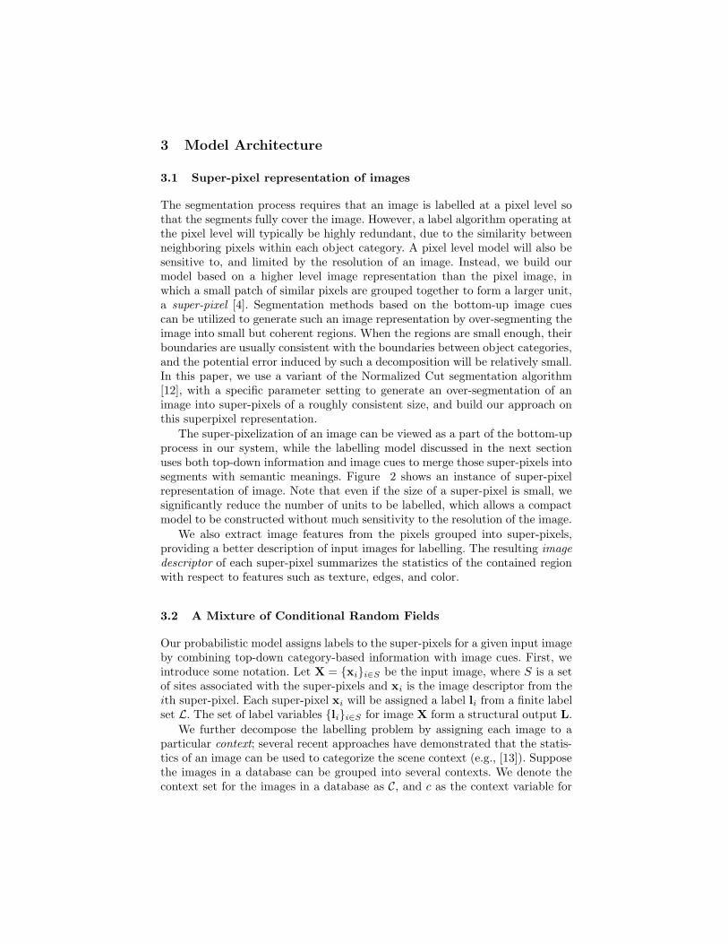
3 Model Architecture

3.1 Super-pixel representation of images

The segmentation process requires that an image is labelled at a pixel level sothat the segments fully cover the image. However, a label algorithm operating atthe pixel level will typically be highly redundant, due to the similarity betweenneighboring pixels within each object category. A pixel level model will also besensitive to, and limited by the resolution of an image. Instead, we build ourmodel based on a higher level image representation than the pixel image, inwhich a small patch of similar pixels are grouped together to form a larger unit,a super-pixel [4]. Segmentation methods based on the bottom-up image cuescan be utilized to generate such an image representation by over-segmenting theimage into small but coherent regions. When the regions are small enough, theirboundaries are usually consistent with the boundaries between object categories,and the potential error induced by such a decomposition will be relatively small.In this paper, we use a variant of the Normalized Cut segmentation algorithm[12], with a specific parameter setting to generate an over-segmentation of animage into super-pixels of a roughly consistent size, and build our approach onthis superpixel representation.

The super-pixelization of an image can be viewed as a part of the bottom-upprocess in our system, while the labelling model discussed in the next sectionuses both top-down information and image cues to merge those super-pixels intosegments with semantic meanings. Figure 2 shows an instance of super-pixelrepresentation of image. Note that even if the size of a super-pixel is small, wesignificantly reduce the number of units to be labelled, which allows a compactmodel to be constructed without much sensitivity to the resolution of the image.

We also extract image features from the pixels grouped into super-pixels,providing a better description of input images for labelling. The resulting image

descriptor of each super-pixel summarizes the statistics of the contained regionwith respect to features such as texture, edges, and color.

3.2 A Mixture of Conditional Random Fields

Our probabilistic model assigns labels to the super-pixels for a given input imageby combining top-down category-based information with image cues. First, weintroduce some notation. Let X = {xi}i∈S be the input image, where S is a setof sites associated with the super-pixels and xi is the image descriptor from theith super-pixel. Each super-pixel xi will be assigned a label li from a finite labelset L. The set of label variables {li}i∈S for image X form a structural output L.

We further decompose the labelling problem by assigning each image to aparticular context; several recent approaches have demonstrated that the statis-tics of an image can be used to categorize the scene context (e.g., [13]). Supposethe images in a database can be grouped into several contexts. We denote thecontext set for the images in a database as C, and c as the context variable for

input image X. Our model defines a conditional distribution over the output Lgiven input X:

P (L|X) =∑

c∈C

PM (L|X, c)PG(c|X) (1)

where PM (L|X, c) is a conditional random field (CRF) for the context c, andPG(c|X) is a gating function which yields the probability distribution of contextgiven the information from image X. We refer to the model in Eqn. 1 as aMixture of Conditional Random Fields (MoCRF). With CRFs as its mixturecomponents, this model can be viewed as an extension of a mixture of expertsmodel [14] by predicting a structural output from data. Below we describe thecomponent CRF models in detail, followed by the gating function.

3.3 Context-dependent conditional random field

Given a context, the model captures the interactions between the labels of animage using a conditional random field of the labels PM (L|X, c). The randomfield is defined with respect to a graph G in which the label sites of neighboringsuper-pixels on the image plane are connected. We denote the neighbors of sitei as N(i).

The context-dependent CRF has three types of feature functions in its dis-tribution, encoding the top-down contextual constraint of the labelling at threelevels:

PM (L|X, c) =1

Zc

exp{∑

i

fa(li,xi, c) +∑

i

∑

j∈N(i)

fb(li, lj , c) + fc(L, c)}, (2)

where fa(li,xi, c) is a feature function describing the compatibility of the localimage descriptor xi at super-pixel i to a particular label variable li; fb(li, lj , c) ac-counts for pairwise interactions between labels of neighboring sites; and fc(L, c)is a feature function for the global statistics of the label field L under context c.In our model, we implement those feature functions as follows:

(a). Local features fa(li,xi, c). We utilize a classifier that independentlypredicts the label of every super-pixel to build the local feature function. Theclassifier provides a label distribution ΦI(li|xi, c) given input xi and context c.The local feature fa(li,xi, c) has the following form:

fa(li,xi, c, γc) = αc

∑

k∈L

δ(li = k) log ΦI(li = k|xi, c, γc), (3)

where δ(x) = 1 if x is true and 0 otherwise, αc is a coefficient for modulatingthe entropy of the classifier output for context c, and γc represents the classifierparameters. The feature function describes the preference of different label con-figurations given the input. In this paper, we use a multilayer perceptron (MLP)as the classifier which takes color, edge magnitude and texture information fromthe ith super-pixel’s descriptor as the input. Note that these feature functions

may be able to find local image features that uniquely characterize a particularclass, such as the combination of color, texture, and edges in a rhino’s horn.

(b). Pairwise features fb(li, lj , c). The pairwise feature functions exploitthe local interactions between labels of neighboring super-pixels. We use a pair-wise feature with a linear form in this model:

fb(li, lj , c) =∑

k∈L

∑

k′∈L

δ(li = k)δ(lj = k′) log Ψ cij(k, k′), (4)

where Ψ cij is a |L|×|L| compatibility matrix between label li and lj . The compat-

ibility matrix incorporates both the statistics of neighboring label configurationsand image descriptor information; it is defined as follows:

Ψ cij(k, k′) =

{

(1 − P bij) exp(θc

k,k′) k = k′

P bij exp(θc

k,k′) k 6= k′ (5)

where θck,k′ is a scalar parameter for the compatibility of label values k, k′ in

context c. This formulation incorporates boundary information provided by aseparate boundary classifier [15]: P b

ij is the boundary probability between super-pixel i and j, which modulates the label pair compatibility, implementing theintuitive notion that the compatibility of labels of neighboring sites depends onthe presence of a boundary between them. For example, one would expect thatthe likelihood of neighboring labels taking on the same value would decrease ifthere is a boundary between them, while the compatibility of taking on differentvalues would decrease if no boundary exists. Therefore, fb(li, lj , c) can be viewedas a data-dependent feature function specifying the regional context of labels.

(c). Global features fc(L, c). The global feature function provide a coarselevel constraint for the label configuration of the random field. In our model,the global features constrain the overall image label distribution to conform toa typical, average label distribution that characterizes the relative proportion ofthe various labels in a specific context. Assuming this average label distribution isµc = (µc

1, ..., µc|L|) for a given context c, we define a global feature that maximizes

the match between the actual label distribution and the distribution µc:

fc(L, c) = βc∑

i

∑

k∈L

δ(li = k) log µck, (6)

where βc is the weighting coefficient. This feature function is equivalent to thenegative Kullback-Leibler divergence between the image label distribution andthe target distribution for the given context. Note that this feature provides aglobal bias to the single node potential in the conditional random field.

3.4 Gating function PG(c|X)

The gating function is specified by a context classifier which generates a distri-bution of context c given an input image. The inputs to the classifier are theaggregate statistics of the image descriptors, including color, edge density andtexture information. We use a multilayer perceptron as the context classifier inthis model.

P(L|X)

Label: L

Image: X

GatingFunction

Σ

BoundaryProbability

BoundaryProbability

Context Feature

Pairwise Feature

Local Feature

Labels

Superpixel Descriptor

Fig. 3. Graphical model representation. Left: The superpixel descriptors are inputto context-specific processing, with the gating function modulating the relevance ofeach context to a given image. Right: The context-specific processing combines localinformation based on super-pixel descriptor and specific label compatibility; pairwiseinteractions between labels of neighboring sites, modulated by the boundary probabil-ity; and global bias provided by the context-specific average label distribution.

3.5 Model summary

To summarize, our model has the following form:

P (L|X) =∑

c

PG(c|X)

Zc

exp{∑

i,j

lTi log Ψ cijlj + αc

∑

i

lTi log ΦI + βc∑

i

lTi log µc}

(7)where the label variable li is represented as a vector with |L| elements, in whichthe kth element is 1 and the other elements are 0 when li = k. Figure 3 providesan overview of the main components of the model. Note that the final labeldistribution can readily be used to define a segmentation of the image intocoherent regions, where a segment corresponds to each contiguous group of pixelsthat are assigned the same label.

4 Image Labeling and Parameter Estimation

4.1 Inference and learning criterion

Given a new image X, we predict its labelling based on the Maximum PosteriorMarginals (MPM) criterion:

l∗i = arg maxli∈L

∑

c∈C

PM (li|X, c)PG(c|X), (8)

where the marginal label distributions of each super-pixel, PM (li|X, c), are com-puted by applying loopy belief propagation to every context-dependent CRF.

Given a set of labeled image data X = {(Ln,Xn)}, we estimate the model’sparameters based on the Conditional Maximum Likelihood criterion, that is,

Θ̂ = arg maxΘ

∑

n

log P (Ln|Xn), (9)

where Θ denotes all the parameters in the model. Treating the context variablec as missing data, we could apply the EM algorithm to the learning problem.However, due to the partition functions in the mixture components, the posteriordistribution q(c|Ln,Xn) is intractable. Instead, we define a new cost functionwhich is a lower-bound of the conditional data likelihood:

Q =∑

n

∑

c

PG(c|Xn) log PM (Ln|Xn, c). (10)

Note that Q ≤∑

n log[∑

c PG(c|Xn)PM (Ln|Xn, c)] =∑

n log P (Ln|Xn).

4.2 A modular training approach

Given the cost function in Eqn. 10, we can compute its gradient and estimate allthe parameters using a gradient ascent method. However, training all parameterstogether becomes difficult in practice when we have a large label set, and largeimage database. In this work, we propose a modular approach to estimate theparameters, such that many components are learned separately and are thenmerged into the full system in a consistent way. This learning procedure maynot produce an optimal system ultimately, but the approach leads to a moreefficient learning process, capable of scaling up to large datasets.

The learning procedure is carried out as follows: (1). We cluster the trainingdata, where each training image is represented by its aggregate label distribu-tion, and define each cluster as a context. The clustering divides the training datainto subsets, such that each image corresponds to a specific context. (2). Giventhis division of training data, we can train the gating function that predictswhich context an image is in given its image features. (3). Within each subset,we estimate the parameters {γc} of each context-dependent image classifier toindependently predict the label distribution given the super-pixel descriptors asinput. (4). Finally, we combine these components and jointly learn the remainingparameters in the model (the coefficients {αc, βc} and the compatibility param-eters θc) by maximizing the cost function in Eqn. 10.

More specifically, in step 1, the clustering method is based on a mixtureof unigram model for the labels: Pu(L) =

∑

c

∏

i Pu(li|c)Pu(c), which we learnusing the EM algorithm on the training data set. The conditional probabilityPu(li|c) acts as the cluster center, or the prototype label distribution in contextc, and is thus used as µc in the global feature function. In step 2, given themixture of unigram model, we can compute the cluster responsibility of everyimage. Those responsibilities are used as training targets for the gating functionPG(c|X). Step 3 can occur in parallel with step 2, as by sampling the responsi-bilities, we can form the context-dependent subsets from the training data, andlearn the parameters γc of the local feature functions on the appropriate subsets.

Finally, in step 4, after parameters of the local and global feature functions aswell as the gating function have been learned, we merge them into the model andoptimize the remaining parameters with respect to the cost function. Note thatthe context-dependent CRFs are log-linear models with parameters {θc, αc, βc},

which can be estimated by gradient ascent:

∆θc ∝ PG(c|Xn)∑

n

∑

i,j∈N(i)

(lni lnTj −

⟨

lilTj

⟩

PM (li,lj |Xn,c)) (11)

∆αc ∝ PG(c|Xn)∑

n

∑

i

(lnTi −

⟨

lTi⟩

PM (li|Xn,c)) log ΦI(li|x

ni , c) (12)

∆βc ∝ PG(c|Xn)∑

n

∑

i

(lnTi −

⟨

lTi⟩

PM (li|Xn,c)) log µc. (13)

To avoid overfitting, we add a Gaussian prior on the parameters, which is equiv-alent to weight decay during learning. As the CRFs are defined on loopy graphswith intractable partition functions, the marginal distributions of the label vari-ables in the gradient updates cannot be computed exactly. In this work, weapproximate them by applying the loopy belief propagation algorithm. An al-ternative approach is to apply contrastive divergence [16] to each componentCRF. The empirical results show that both of these approaches obtain similarand satisfactory performance in our model; below we report results using loopybelief propagation.

5 Experimental Evaluation

5.1 Data sets

We applied our model to three different real data sets. In order to compareour method with an alternative approach, we utilized the two datasets usedin our mCRF work [11], and used the same training and testing split as inthat work. The first dataset is the Sowerby database, including a set of colorimages of outdoor scenes and their associated labels. The data set has a totalof 104 images with 7 labels: ’sky’, ’vegetation’, ’road marking’, ’road surface’,’building’, ’street objects’ and ’cars’. 60 of these images are used for training andthe remaining 44 for testing. The second dataset is a 100-image subset of theCorel image database, consisting of African and Arctic wildlife natural scenes. Italso has 7 classes: ’rhino/hippo’, ’polar bear’, ’vegetation’, ’sky’, ’water’, ’snow’and ’ground’; and has a train/test split of 60/40.

To explore the scaling potential of our approach, we defined a third datasetby expanding this Corel dataset to include 305 manually labelled images with11 classes: ’rhino/hippo’, ’tiger’, ’horse’,’polar bear’, ’wolf/leopard’, ’vegetation’,’sky’, ’water’, ’snow’, ’ground’ and ’fence’. The training set includes 229 ran-domly selected images and the remaining 76 are used for testing. We call thisextended Corel data set CorelB, and refer to the smaller one as CorelA in thefollowing sections.

Again, for comparison purposes, we use the same set of basic image features asin [11], including color, edge and texture information. For the color information,we transform the RGB values into CIE Lab* color space, which is perceptuallyuniform. The edge and texture are extracted by a set of filter-banks including a

difference-of-Gaussian filter at 3 different scales, and quadrature pairs of orientedeven- and odd-symmetric filters at 4 orientations (0; π/4; π/2; 3π/4) and 3 scales.We also include the vertical and horizontal position of each pixel. Thus eachpixel is represented by a 32 dimensional image feature vector. For super-pixels,we compute the normalized histograms of those image features extracted fromthe pixels in each super-pixel.

5.2 Model specification

We use the normalized cut segmentation algorithm to build the super-pixel rep-resentation of the images, in which the segmentation algorithm is tuned to gen-erate more than 300 segments for each image. Segments smaller than a minimumsize (6 pixels) are merged into the neighboring super-pixels. This yields approx-imately 300 super-pixels per image on average. The boundary information isextracted using the algorithm in [15]. To avoid underflow, we convert the rawoutput of boundary probability into interval [0.1, 0.9] by an affine transform.

The number of contexts in our experiments is specified based on the com-plexity of data set. For Sowerby and CorelA data sets, we use 2 contexts inclustering, and for CorelB, we use 4 contexts. The model selection issue is notexplored here, and is left to future work.

The gating function is a MLP with 25 hidden units. It takes the normalizedhistograms of the image features in each image as input. We use 20 bins for eachimage feature. To avoid overfitting, the MLP is trained with Gaussian priorson weights. The local classifiers are also MLPs with 30 hidden units, using thehistograms of the image features in each super-pixel as input. They are trainedwith cross-validation.

We compare our approach with a simple pixel-wise classifier and a CRFmodel. These comparisons provide insight into the utility of the pairwise com-patibilities (CRF vs. classifier) and the contexts (MoCRF vs. CRF). The pixel-wise classifier is a MLP with one hidden layer, taking image features from a 3×3window centered at each pixel and predicting the pixel’s label. The CRF usescontext-independent local feature and pairwise feature functions. The featurefunctions have the same form as our model. The distribution of label configura-tion L defined by the CRF has the following form:

PCRF (L|X) =1

Zexp{

∑

i,j

lTi log Ψijlj + α∑

i

lTi log ΦI(li|xi)} (14)

where ΦI is a local classifier trained separately on all the data and Ψij is thecompatibility function including boundary information. We trained the CRFmodel using the pseudo-likelihood algorithm, and tested its performance usingthe same MPM criterion where the marginal distribution is calculated by theloopy belief propagation algorithm.

Hippo/Rhino

Polar Bear

Water

Snow

Vegetaion

Ground

Sky

Sky

Vegetation

Road Mark

Road Surface

Ground

Street Obj

Car

Hippo/Rhino

Horse

Tigher

Polar Bear

Wolf/Lepard

Water

Vegetaion

Sky

Ground

Snow

Fence

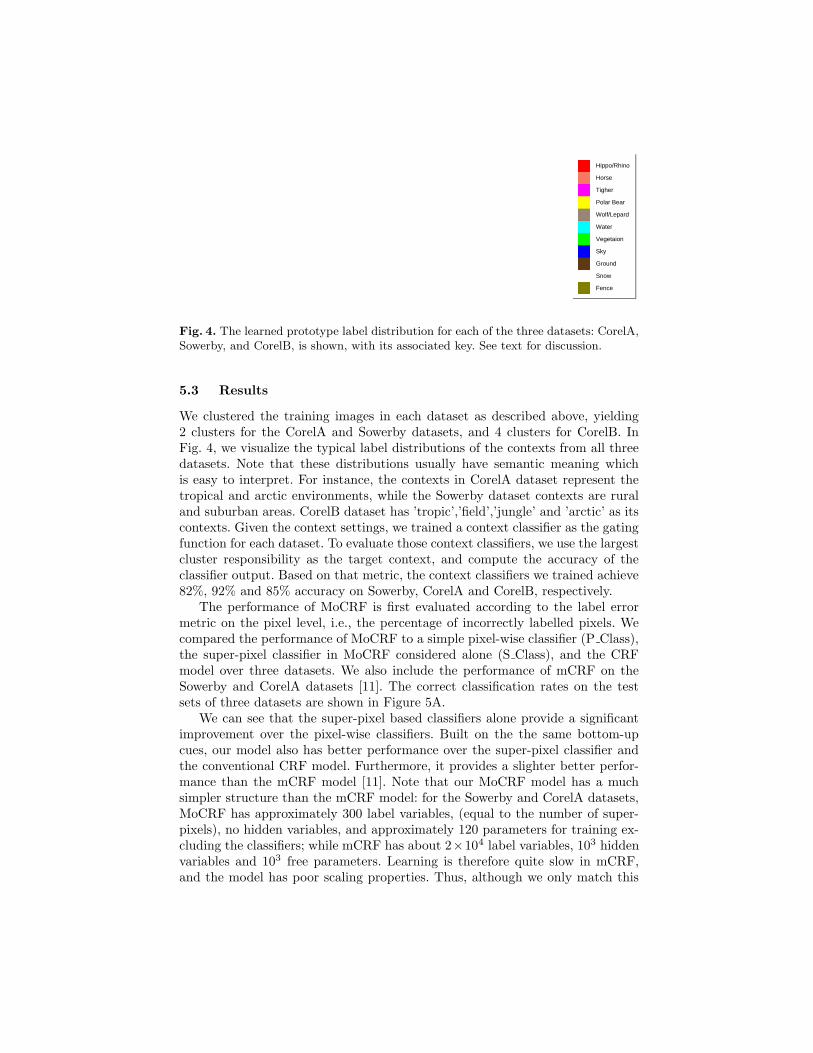
Fig. 4. The learned prototype label distribution for each of the three datasets: CorelA,Sowerby, and CorelB, is shown, with its associated key. See text for discussion.

5.3 Results

We clustered the training images in each dataset as described above, yielding2 clusters for the CorelA and Sowerby datasets, and 4 clusters for CorelB. InFig. 4, we visualize the typical label distributions of the contexts from all threedatasets. Note that these distributions usually have semantic meaning whichis easy to interpret. For instance, the contexts in CorelA dataset represent thetropical and arctic environments, while the Sowerby dataset contexts are ruraland suburban areas. CorelB dataset has ’tropic’,’field’,’jungle’ and ’arctic’ as itscontexts. Given the context settings, we trained a context classifier as the gatingfunction for each dataset. To evaluate those context classifiers, we use the largestcluster responsibility as the target context, and compute the accuracy of theclassifier output. Based on that metric, the context classifiers we trained achieve82%, 92% and 85% accuracy on Sowerby, CorelA and CorelB, respectively.

The performance of MoCRF is first evaluated according to the label errormetric on the pixel level, i.e., the percentage of incorrectly labelled pixels. Wecompared the performance of MoCRF to a simple pixel-wise classifier (P Class),the super-pixel classifier in MoCRF considered alone (S Class), and the CRFmodel over three datasets. We also include the performance of mCRF on theSowerby and CorelA datasets [11]. The correct classification rates on the testsets of three datasets are shown in Figure 5A.

We can see that the super-pixel based classifiers alone provide a significantimprovement over the pixel-wise classifiers. Built on the the same bottom-upcues, our model also has better performance over the super-pixel classifier andthe conventional CRF model. Furthermore, it provides a slighter better perfor-mance than the mCRF model [11]. Note that our MoCRF model has a muchsimpler structure than the mCRF model: for the Sowerby and CorelA datasets,MoCRF has approximately 300 label variables, (equal to the number of super-pixels), no hidden variables, and approximately 120 parameters for training ex-cluding the classifiers; while mCRF has about 2×104 label variables, 103 hiddenvariables and 103 free parameters. Learning is therefore quite slow in mCRF,and the model has poor scaling properties. Thus, although we only match this

Corel A Corel B Sowerby60

65

70

75

80

85

90

95P_ClassS_ClassCRFmCRFMoCRF

Corel A Corel B Sowerby60

65

70

75

80

85

90

95Mean−ShiftS_ClassCRFMoCRF

Fig. 5. A (left): Classification rates; B (right): Segmentation accuracy for the models.

earlier model in terms of classification accuracy, our model can be applied to theproblems with a considerably larger set of labels and larger image sizes.

We compare the performance of the pixel-wise classifier, our model, andMean-Shift segmentation in Figure 5B. We tune the parameters of Mean-Shiftsuch that it generates the best results according to the manual labeling for asmall set of randomly chosen images. The performance is measured according toa second metric used for evaluation, a segmentation metric which computes thepercentage of pixel pairs that are correctly segmented. To reduce the compu-tational burden, we randomly sampled 10% pixels from each image to estimatethe accuracy. Again, we can see that our model obtains better results by addingtop-down category information, and multi-level contextual constraints.

We also show the outputs of these methods on some test images in Figure6. The figure shows the approaches based solely on low-level cues can be fooled,such that some single objects in the images are split. MoCRF works much betteron those images by integrating the super-pixel representation and mixture ofCRF framework. Note that the super-pixelization will cause some errors whichcannot be corrected by the top-down information. Also, the model cannot useglobal spatial configuration to correct errors since no geometric information isincluded in the global feature functions.

6 Discussion

In this paper we have presented a discriminative framework that integratesbottom-up and top-down cues for image segmentation. We adopt a labellingapproach to provide some purchase on the segmentation problem. A chief con-tribution of our model with respect to segmentation is the resulting extension oftop-down cues to include a considerably wider range of object classes than earliermethods. The proposed framework is modular, in that images in a database areclassified as to their context, and separate processes are learned for the differ-ent contexts. This modularity presents some promise of the system extending to

Original Hand-labeling Classifier MoCRF Mean-Shift

Fig. 6. Some labeling results for the Corel (4 top rows) and Sowerby (2 bottom rows)datasets, using the pixel-wise classifier, CRF, MoCRF, and Mean Shift segmentation.The color keys for the labels are the same as Fig. 4.

large databases of images. While the top-down cues can be learned in a context-specific manner, the system integrates these with bottom-up cues, which areutilized in several ways: to define super-pixels in an image; to determine prob-abilities of local boundaries between super-pixels, which are used to constrainand guide labelling; and to enable context classification.

The results of applying our method to three different image datasets sug-gest that this integrated approach may extend to a variety of image types anddatabases. The labeling system consistently out-performs alternative approaches,such as a standard classifier and a standard CRF. Its performance matches thatof an existing method, which operates at the pixel level and entails a consider-ably more involved training procedure, one which is unlikely to scale to largerimages and image databases. Relative to a standard segmentation method, thesegmentations produced by our method are more accurate, even when the stan-dard method is optimized for a given test image. A relatively weak componentin our model appears to be the gating function, as the images whose contexts

are incorrectly classified contain a disproportionate number of label errors. Weare currently evaluating other methods of summarizing the statistics of an imagein order to facilitate more accurate context classification. Finally, a limitationof our model concerns its reliance on detailed training data. However, a growingeffort to label images (e.g., [17]) should lead to a rapid growth in the volume ofavailable labeled images.

Acknowledgments

We thank BAE Systems for letting us use their Sowerby Image Database. Fundedby grants from Communications and Information Technology Ontario and NSERC.

References

1. Peterson, M., Gibson, B.: Shape recognition contributions to figure-ground orga-nization in three-dimensional displays. Cognitive Psychology 25 (1993) 383–429.

2. Lafferty, J., McCallum, A., Pereira, F.: Conditional random fields: Probabilisticmodels for segmenting and labeling sequence data. In: Proc. 18th ICML. (2001).

3. Kumar, S., Hebert, M.: Discriminative random fields: A discriminative frameworkfor contextual interaction in classification. In: ICCV. (2003).

4. Ren, X., Malik, J.: Learning a classification model for segmentation. In: ICCV.(2003).

5. Liu, L., Sclaroff, S.: Region segmentation via deformable model-guided split andmerge. In: ICCV. (2001).

6. Borenstein, E., Sharon, E., Ullman, S.: Combining top-down and bottom-up seg-mentation. In: Proceedings IEEE Workshop of Perceptual Organization in Com-puter Vision. (2004).

7. Yu, S., Shi, J.: Object-specific figure-ground segregation. In: CVPR. (2003).8. Tu, Z., Chen, X., Yuille, A., Zhu, S.C.: Image parsing: Unifying segmentation,

detection, and object recognition. International Journal of Computer Vision 63

(2005) 113–140.9. Murphy, K., Torralba, A., Freeman, W.: Using the forest to see the trees: A

graphical model relating features, objects and scenes. In: NIPS-04. (2004).10. Carbonetto, P., de Freitas, N., Barnard, K.: A statistical model for general con-

textual object recognition. In: ECCV. (2004).11. He, X., Zemel, R., Carreira-Perpinan, M.: Multiscale conditional random fields for

image labelling. In: CVPR. (2004).12. Shi, J., Malik, J.: Normalized cuts and image segmentation. IEEE Trans. PAMI

22 (2000) 888–905.13. Torralba, A., Oliva, A.: Statistics of natural image categories. Network: Compu-

tation in neural systems 14 (2003) 391–412.14. Jacobs, R.A., Jordan, M.I., Nowlan, S., Hinton, G.E.: Adaptive mixtures of local

experts. Neural Computation 3 (1991) 1–12.15. Martin, D., Fowlkes, C., Malik, J.: Learning to detect natural image boundaries

using local brightness, color and texture cues. IEEE Trans. PAMI. 26 (2003)530–549.

16. Hinton, G.E.: Training products of experts by minimizing contrastive divergence.Neural Computation 14 (2002) 1771–1800.

17. Russell, B., Torralba, A., Murphy, K., Freeman, W.: LabelMe: A database andweb-based tool for image annotation (2005).