Embed Size (px)
Citation preview

Leakage in Trustworthy Systems
David Cock
Submitted in fulfilment of the requirements for the degree ofDoctor of Philosophy
School of Computer Science and Engineering
Faculty of Engineering
August 2014

Originality Statement
‘I hereby declare that this submission is my own work and to the best ofmy knowledge it contains no materials previously published or written byanother person, or substantial proportions of material which have been ac-cepted for the award of any other degree or diploma at UNSW or any othereducational institution, except where due acknowledgement is made in thethesis. Any contribution made to the research by others, with whom I haveworked at UNSW or elsewhere, is explicitly acknowledged in the thesis. Ialso declare that the intellectual content of this thesis is the product of myown work, except to the extent that assistance from others in the project’sdesign and conception or in style, presentation and linguistic expression isacknowledged.’
Signed . . . . . . . . . . . . . . . . . . . . . . . . . . . . . . . . . . . . . . . . . . . . . . . . . . . . . . . . . . . . . . . . . .
Date . . . . . . . . . . . . . . . . . . . . . . . . . . . . . . . . . . . . . . . . . . . . . . . . . . . . . . . . . . . . . . . . . . . .
ii

Copyright Statement
‘I hereby grant the University of New South Wales or its agents the right toarchive and to make available my thesis or dissertation in whole or part in theUniversity libraries in all forms of media, now or here after known, subject tothe provisions of the Copyright Act 1968. I retain all proprietary rights, suchas patent rights. I also retain the right to use in future works (such as articlesor books) all or part of this thesis or dissertation. I also authorise UniversityMicrofilms to use the 350 word abstract of my thesis in Dissertation AbstractInternational (this is applicable to doctoral theses only). I have either usedno substantial portions of copyright material in my thesis or I have obtainedpermission to use copyright material; where permission has not been grantedI have applied/will apply for a partial restriction of the digital copy of mythesis or dissertation.’
Signed . . . . . . . . . . . . . . . . . . . . . . . . . . . . . . . . . . . . . . . . . . . . . . . . . . . . . . . . . . . . . . . . . .
Date . . . . . . . . . . . . . . . . . . . . . . . . . . . . . . . . . . . . . . . . . . . . . . . . . . . . . . . . . . . . . . . . . . . .
Authenticity Statement
‘I certify that the Library deposit digital copy is a direct equivalent of thefinal officially approved version of my thesis. No emendation of content hasoccurred and if there are any minor variations in formatting, they are theresult of the conversion to digital format.’
Signed . . . . . . . . . . . . . . . . . . . . . . . . . . . . . . . . . . . . . . . . . . . . . . . . . . . . . . . . . . . . . . . . . .
Date . . . . . . . . . . . . . . . . . . . . . . . . . . . . . . . . . . . . . . . . . . . . . . . . . . . . . . . . . . . . . . . . . . . .
iii

iv
Abstract
This dissertation presents a survey of the theoretical and prac-tical techniques necessary to provably eliminate side-channel leak-age through known mechanisms in component-based secure sys-tems.
We cover the state of the art in leakage measures, includingboth Shannon and min entropy, concluding that Shannon entropymodels the observed behaviour of our example systems closely,and can be used to give a safe bound on vulnerability in practicalscenarios.
We comprehensively analyse several channel-mitigation strate-gies: cache colouring and instruction-based scheduling, showingthat effectiveness and ease of implementation depend stronglyon subtle hardware features. We also demonstrate that real-timescheduling can be employed to effectively mitigate remote chan-nels at minimal cost.
Finally, we demonstrate that we can reason formally (and me-chanically) about probabilistic non-functional properties, by for-malising the probabilistic language pGCL in the Isabelle/HOLtheorem prover, and using it to verify an implementation of lat-tice scheduling, a well-known cache-channel countermeasure. Weprove that a correspondence exists between standard vulnerabilitybounds, in a channel-centric view, and the refinement lattice onprograms in pGCL, used to model a guessing attack on a vulnera-ble system—a process-centric view.

v
For Fiona, Lillian and Frederick; and my parents.
Contents
Originality Statement ii
Copyright Statement iii
Authenticity Statement iii
Contents vi
List of Figures viii
List of Tables xii
List of Publications xiii
1 Introduction 1
2 Covert and Side Channels 52.1 Background . . . . . . . . . . . . . . . . . . . . . . . . . . . . . 62.2 The strcmp Channel . . . . . . . . . . . . . . . . . . . . . . . . 112.3 Leakage with a Uniform Prior . . . . . . . . . . . . . . . . . . . 122.4 Leakage with a Nonuniform Prior . . . . . . . . . . . . . . . . 242.5 Reevaluating Shannon Entropy . . . . . . . . . . . . . . . . . . 332.6 Noisy Channels & Information Theory . . . . . . . . . . . . . . 372.7 A Safe Leakage Model for strcmp . . . . . . . . . . . . . . . . . 442.8 Related Work . . . . . . . . . . . . . . . . . . . . . . . . . . . . 492.9 Summary . . . . . . . . . . . . . . . . . . . . . . . . . . . . . . . 50
3 Case Study: Practical Countermeasures 533.1 Experimental Setup . . . . . . . . . . . . . . . . . . . . . . . . . 543.2 The Local Channels . . . . . . . . . . . . . . . . . . . . . . . . . 60
vi

CONTENTS vii
3.3 Cache Colouring . . . . . . . . . . . . . . . . . . . . . . . . . . 683.4 Noise versus Determinism . . . . . . . . . . . . . . . . . . . . . 783.5 Instruction-Based Scheduling . . . . . . . . . . . . . . . . . . . 793.6 Lucky thirteen as a Remote Channel . . . . . . . . . . . . . . . 883.7 Scheduled Message Delivery . . . . . . . . . . . . . . . . . . . 913.8 Related Work . . . . . . . . . . . . . . . . . . . . . . . . . . . . 963.9 Conclusions . . . . . . . . . . . . . . . . . . . . . . . . . . . . . 98
4 pGCL for Systems 1034.1 The Case for Probabilistic Correctness . . . . . . . . . . . . . . 1044.2 The pGCL Language . . . . . . . . . . . . . . . . . . . . . . . . 1074.3 The pGCL Theory Package . . . . . . . . . . . . . . . . . . . . . 1104.4 Implementation and Extensions . . . . . . . . . . . . . . . . . . 1164.5 Related Work . . . . . . . . . . . . . . . . . . . . . . . . . . . . 1214.6 Summary . . . . . . . . . . . . . . . . . . . . . . . . . . . . . . . 123
5 Case Study: Lattice Scheduling 1255.1 Security Policies and Covert Channels . . . . . . . . . . . . . . 1265.2 Countermeasures through Refinement . . . . . . . . . . . . . . 1275.3 Ongoing & Future Work . . . . . . . . . . . . . . . . . . . . . . 1395.4 Related Work . . . . . . . . . . . . . . . . . . . . . . . . . . . . 1405.5 Summary . . . . . . . . . . . . . . . . . . . . . . . . . . . . . . . 141
6 Formal Leakage Models 1436.1 An Informal Model . . . . . . . . . . . . . . . . . . . . . . . . . 1456.2 A Formal Model . . . . . . . . . . . . . . . . . . . . . . . . . . . 1486.3 Simpler Bounds using Refinement . . . . . . . . . . . . . . . . 1556.4 Related Work . . . . . . . . . . . . . . . . . . . . . . . . . . . . 1626.5 Summary . . . . . . . . . . . . . . . . . . . . . . . . . . . . . . . 164
7 Conclusion 165
A Detailed Proofs 167
Bibliography 175

List of Figures
2.1 strcmp, from GNU glibc 2.9 (edited for readability). . . . . . . . . 10
2.2 Vulnerability (V0) vs. number of guesses (k), for strcmp with noside channel, wherem = 3, n = 3. . . . . . . . . . . . . . . . . . . 13
2.3 strcmp attack traces with leakage for m = 3, n = 3, showingvulnerability (V0) vs. number of guesses (k), and log2 P(V0|k) ateach vertex. Includes the no-leakage trace in blue for comparison 15
2.4 strcmp attack traces form = 6, n = 6, showing vulnerability (V0)vs. number of guesses (k), and log2 P(V0|k) at each vertex. Includesthe 10th, 50th and 90th percentiles for P(V0|k). . . . . . . . . . . . 15
2.5 k-guess vulnerability (Vk) vs. k, for m = 6,n = 6, together withexpected one-guess vulnerability (V0(k)). Also shown are the ex-pected uncertainty set size (E(1/V0(k))), and the linear trend as-suming 1 position is found every 3 guesses, showing roughlylog-linear behaviour. . . . . . . . . . . . . . . . . . . . . . . . . . . 19
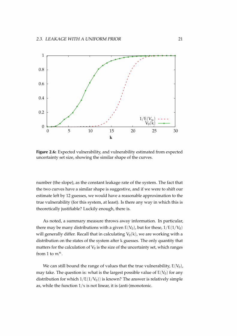
2.6 Expected vulnerability, and vulnerability estimated from expecteduncertainty set size, showing the similar shape of the curves. . . . 21
2.7 Pessimistic correction of the uncertainty-set measure. . . . . . . . 23
2.8 An attack state (m = 3,n = 4) represented as a tree. Every pathfrom the root is a possible secret. The prefix ‘ca’ has been estab-lished. The edge from sj−1 to sj is labelled with P(sj|sj−1, . . . , s1).The leaves are labelled with the probability of the path that leadsto them, or P(sj, . . . , s1) . . . . . . . . . . . . . . . . . . . . . . . . . 28
2.9 The attack in Figure 2.8 after guessing ‘caaa’ and seeing a prefixlength of 2. The left subtree has been eliminated, and the condi-tional probabilities of the others adjusted, changing the probabili-ties at the leaves. . . . . . . . . . . . . . . . . . . . . . . . . . . . . 28
viii

List of Figures ix
2.10 The attack in Figure 2.8 after guessing ‘caaa’ and seeing a prefixlength of 3. The middle and right subtrees have been eliminated,as has the subtree rooted at ‘caaa’. . . . . . . . . . . . . . . . . . . 29
2.11 The attack in Figure 2.8 after guessing correctly that position j is‘a’, and that position j+ 1 is ‘b’. The middle and right subtrees havebeen eliminated, as have ‘a’ and ‘c’ in the final row. . . . . . . . . 29
2.12 Comparison of one-guess vulnerability (V0) and expected entropy(H1) for a uniform, and a Markov prior. m = 6,n = 6. . . . . . . . 31
2.13 Graph of Equation 2.13, showing maximum at V0 = 1/8,H1 = 3.N = 8. . . . . . . . . . . . . . . . . . . . . . . . . . . . . . . . . . . . 35
2.14 Pessimistic correction function, K8, derived from Figure 2.13. . . . 36
2.15 Worst-case expected one-guess vulnerability given H1 entropy, fora distribution over 66 secrets, showing nearly linear behaviour. . . 36
2.16 Expected vulnerability and entropy for m = 6,n = 6, showingboth a naïve vulnerability estimate, and its safe correction. . . . . 37
2.17 strcmp execution time distribution, via RPC over the Linux net-working stack, showing probability density (ρ). . . . . . . . . . . . 39
2.18 Channel matrix for strcmp leakage. C = 2.34× 10⁻³b. . . . . . . . 40
2.19 Intrinsic leakage showing both vulnerability and entropy, con-trasted with leakage including the side channel. . . . . . . . . . . 41
2.20 Increase in leakage due to the strcmp side channel, includingforced exponential model. Also shown is the maximum possibleleakage given channel capacity. . . . . . . . . . . . . . . . . . . . . 43
2.21 Entropy differential for simulated channel matrices of varyingcapacity, bounded by the intrinsic entropy and showing asymptoticbehaviour. . . . . . . . . . . . . . . . . . . . . . . . . . . . . . . . . 44
2.22 Differential leakage contrasted with forced exponential model. . . 46
2.23 Detail of Figure 2.22, showing behaviour near k = 0. . . . . . . . . 47
2.24 Vulnerability and expected entropy for m = 6,m = 6, includingside-channel leakage. Shows vulnerability estimated from trueentropy, entropy estimated using uncorrelated model and derivedvulnerability estimate. . . . . . . . . . . . . . . . . . . . . . . . . . 47
2.25 Detail of Figure 2.24, showing low guess numbers. Includes themin-leakage bound for comparison. . . . . . . . . . . . . . . . . . 48

x List of Figures
3.1 iMX.31 cache channel, no countermeasure. C = 4.25b. 7000 sam-ples per column. . . . . . . . . . . . . . . . . . . . . . . . . . . . . . 56
3.2 iMX.31 cache channel, partitioned. C = 2.14 × 10⁻²b, CImax0 =
1.13× 10⁻²b. 63,972 samples per column. . . . . . . . . . . . . . . 58
3.3 Capacity of sampled Exynos4412 cache-channel matrices (parti-tioned), using 7200 samples per column. . . . . . . . . . . . . . . . 58
3.4 Distribution of capacities for 64 simulated zero-capacity matricesderived from Figure 3.2. . . . . . . . . . . . . . . . . . . . . . . . . 59
3.5 The cache-contention channel. . . . . . . . . . . . . . . . . . . . . . 61
3.6 Code to exploit a cache channel. . . . . . . . . . . . . . . . . . . . . 62
3.7 AM3358 cache channel, no countermeasure. C = 4.69b. 6000samples per column. . . . . . . . . . . . . . . . . . . . . . . . . . . 63
3.8 DM3730 cache channel, no countermeasure. C = 5.28b. 8000samples per column. . . . . . . . . . . . . . . . . . . . . . . . . . . 64
3.9 Exynos4412 cache channel, no countermeasure. C = 7.04b. 1000samples per column. . . . . . . . . . . . . . . . . . . . . . . . . . . 65
3.10 E6550 cache channel, no countermeasure. C = 8.82b. 1000 samplesper column. . . . . . . . . . . . . . . . . . . . . . . . . . . . . . . . 66
3.11 Channel capacity against L2 cache size in lines. . . . . . . . . . . . 67
3.12 E6550 bus channel, no countermeasure. C = 5.80 5.815.80b. 3000 sam-
ples per column. . . . . . . . . . . . . . . . . . . . . . . . . . . . . 67
3.13 Cache colouring. . . . . . . . . . . . . . . . . . . . . . . . . . . . . 69
3.14 AM3358 cache channel, partitioned. C = 1.51 × 10⁻²b. CImax0 =
8.10× 10⁻³b. 49,600 samples per column. . . . . . . . . . . . . . . 71
3.15 DM3730 cache channel, partitioned. C = 5.02 5.025.01× 10−3b. CImax
0 =
2.75× 10⁻³b. 63,200 samples per column. . . . . . . . . . . . . . . 71
3.16 DM3730 cache channel, partitioned, showing L1 contention. . . . 72
3.17 Exynos4412 cache channel, partitioned. C = 8.138.148.12 × 10−2b.
CImax0 = 4.37× 10⁻²b. 7200 samples per column. . . . . . . . . . . 73
3.18 Exynos4412 TLB contention. . . . . . . . . . . . . . . . . . . . . . . 74
3.19 E6550 cache channel, partitioned. C = 4.54 × 10⁻¹b. CImax0 =
2.53× 10⁻¹b. 4836 samples per column. . . . . . . . . . . . . . . . 75
3.20 DM3730 cache channel, partitioned, with the receiver’s workingset restricted to 1024 lines. 2000 samples per column. . . . . . . . 76
3.21 DM3730 cache channel, unmitigated, with the receiver’s workingset restricted to 1024 lines. 2000 samples per column. . . . . . . . 77

List of Figures xi
3.22 The effect of correlated versus anticorrelated noise on channelcapacity. . . . . . . . . . . . . . . . . . . . . . . . . . . . . . . . . . 78
3.23 Disassembled machine code corresponding to lines 9–12 of thecache channel exploit in Figure 3.6. . . . . . . . . . . . . . . . . . . 80
3.24 iMX.31 cache channel, instruction-based scheduling. C = 2.12×10⁻⁴b. CImax
0 = 5.41× 10⁻⁵b. 10,000 samples per column. . . . . 81
3.25 AM3358 cache channel, instruction-based scheduling. C = 1.86×10⁻³b. CImax
0 = 9.56× 10⁻⁴b. 10,000 samples per column. . . . . 82
3.26 DM3730 cache channel, instruction-based scheduling. C = 1.49×10⁻³b. CImax
0 = 7.74× 10⁻⁴b. 10,000 samples per column. . . . . 83
3.27 Exynos4412 cache channel, instruction-based scheduling. C =
1.19b. CImax0 = 3.76× 10⁻³b. 1000 samples per column. . . . . . . 84
3.28 Code to test PMU accuracy in the presence of L2 cache misses. . . 85
3.29 Exynos4412 cache channel, instruction-based scheduling and parti-tioning. C = 2.32× 10⁻²b. CImax
0 = 2.78× 10⁻²b. 500 samples percolumn. . . . . . . . . . . . . . . . . . . . . . . . . . . . . . . . . . 86
3.30 E6550 cache channel, instruction-based scheduling. C = 5.71 ×10⁻¹b. CImax
0 = 3.41× 10⁻²b. 600 samples per column. . . . . . . 86
3.31 E6550 bus channel, relaxed determinism. C = 2.90×10⁻¹b. CImax0 =
7.90× 10⁻³b. 3000 samples per column. . . . . . . . . . . . . . . . 87
3.32 Histogram of DTLS echo times for OpenSSL 1.0.1c, at interconti-nental distance—13 hops and 12, 000km, see row 4 of Table 3.2.Generated from 105 samples per packet, and binned at 10µs. Thesepeaks are distinguishable with 62.4% probability. . . . . . . . . . . 90
3.33 Scheduled delivery for OpenSSL. Solid lines are packet flow withdotted control flow. Server blocks at C (call), until R (reply), afterat least ∆t. . . . . . . . . . . . . . . . . . . . . . . . . . . . . . . . . 93
3.34 DTLS distinguishing attack—histogram of response times for packetM0 versus M1. Shows distinguishable peaks for vulnerable imple-mentation in OpenSSL 1.0.1c (VL), constant time implementationin 1.0.1e (CT), and results with scheduled delay (SD) demonstrat-ing reduced latency. All curves generated from 106 packets forbothM0 andM1, and binned at 1µs. . . . . . . . . . . . . . . . . . 94
3.35 Load performance and overhead of scheduled delivery againstunmodified OpenSSL 1.0.1c, and the constant-time implementationof 1.0.1e. . . . . . . . . . . . . . . . . . . . . . . . . . . . . . . . . . 95

4.1 The expectation-transformer interpretation for both wp and wlp. 1114.2 The Monty Hall game in pGCL. . . . . . . . . . . . . . . . . . . . . 1134.3 The underlying definitions of selected pGCL primitives. . . . . . 1174.4 The L4.verified non-deterministic monad in Isabelle. . . . . . . . . 118
5.1 The classification/clearance lattice. . . . . . . . . . . . . . . . . . . 1265.2 The scheduling graph: S. . . . . . . . . . . . . . . . . . . . . . . . . 1275.3 The transition graph: T . . . . . . . . . . . . . . . . . . . . . . . . . 1285.4 First refinement diagram. . . . . . . . . . . . . . . . . . . . . . . . 1315.5 Second refinement diagram. . . . . . . . . . . . . . . . . . . . . . . 1335.6 Composed refinement diagram. . . . . . . . . . . . . . . . . . . . . 1345.7 A schematic depiction of flow from between domains, via shared
state S. . . . . . . . . . . . . . . . . . . . . . . . . . . . . . . . . . . 1375.8 The complete refinement diagram. . . . . . . . . . . . . . . . . . . 139
6.1 The lattice of bounds. . . . . . . . . . . . . . . . . . . . . . . . . . . 163
List of Tables
3.1 Experimental platforms. . . . . . . . . . . . . . . . . . . . . . . . . 553.2 Vulnerability against network distance. . . . . . . . . . . . . . . . 90
xii

List of Publications
• Philip Derrin, Kevin Elphinstone, Gerwin Klein, David Cock, and ManuelM. T. Chakravarty. Running the manual: An approach to high-assurancemicrokernel development. In Proceedings of the ACM SIGPLAN HaskellWorkshop, Portland, OR, USA, September 2006. ACM. doi:10.1145/
1159842.1159850
• David Cock. Bitfields and tagged unions in C: Verification throughautomatic generation. In Bernhard Beckert and Gerwin Klein, editors,Proceedings of the 5th International Verification Workshop, volume 372 ofCEUR Workshop Proceedings, pages 44–55, Sydney, Australia, August2008
• David Cock, Gerwin Klein, and Thomas Sewell. Secure microker-nels, state monads and scalable refinement. In Otmane Ait Mohamed,César Mu noz, and Sofiène Tahar, editors, Proceedings of the 21st Interna-tional Conference on Theorem Proving in Higher Order Logics, pages 167–182,Montreal, Canada, August 2008. Springer.doi:10.1007/978-3-540-71067-7_16
• Simon Winwood, Gerwin Klein, Thomas Sewell, June Andronick, DavidCock, and Michael Norrish. Mind the gap: A verification framework forlow-level C. In Stefan Berghofer, Tobias Nipkow, Christian Urban, andMakarius Wenzel, editors, Proceedings of the 22nd International Conferenceon Theorem Proving in Higher Order Logics, volume 5674 of Lecture Notesin Computer Science, pages 500–515, Munich, Germany, August 2009.Springer. doi:10.1007/978-3-642-03359-9_34
• Gerwin Klein, Kevin Elphinstone, Gernot Heiser, June Andronick, DavidCock, Philip Derrin, Dhammika Elkaduwe, Kai Engelhardt, Rafal Kolan-ski, Michael Norrish, Thomas Sewell, Harvey Tuch, and Simon Win-wood. seL4: Formal verification of an OS kernel. In Proceedings of the
xiii

xiv LIST OF PUBLICATIONS
22nd ACM Symposium on Operating Systems Principles, pages 207–220, BigSky, MT, USA, October 2009. ACM. doi:10.1145/1629575.1629596
• Gerwin Klein, June Andronick, Kevin Elphinstone, Gernot Heiser, DavidCock, Philip Derrin, Dhammika Elkaduwe, Kai Engelhardt, Rafal Kolan-ski, Michael Norrish, Thomas Sewell, Harvey Tuch, and Simon Win-wood. seL4: Formal verification of an operating system kernel. Commu-nications of the ACM, 53(6):107–115, June 2010. doi:10.1145/1743546.
1743574
• David Cock. Lyrebird – assigning meanings to machines. In GerwinKlein, Ralf Huuck, and Bastian Schlich, editors, Proceedings of the 5thSystems Software Verification, pages 1–9, Vancouver, Canada, October2010. USENIX
• David Cock. Exploitation as an inference problem. In Proceedings of the4th ACM Workshop on Artificial Intelligence and Security, pages 105–106,Chicago, IL, USA, October 2011. ACM. doi:10.1145/2046684.2046702
• David Cock. Verifying probabilistic correctness in Isabelle with pGCL.In Proceedings of the 7th Systems Software Verification, pages 1–10, Syd-ney, Australia, November 2012. Electronic Proceedings in TheoreticalComputer Science. doi:10.4204/EPTCS.102.15
• David Cock. Practical probability: Applying pGCL to lattice scheduling.In Proceedings of the 4th International Conference on Interactive TheoremProving, pages 1–16, Rennes, France, July 2013. Springer. doi:10.1007/978-3-642-39634-2_23
• David Cock. From probabilistic operational semantics to informationtheory; side channels in pGCL with isabelle. In Proceedings of the 5thInternational Conference on Interactive Theorem Proving, pages 1–15, Vienna,Austria, July 2014. Springer. doi:10.1007/978-3-319-08970-6_12
• David Cock, Qian Ge, Toby Murray, and Gernot Heiser. The last mile;an empirical study of timing channels on sel4. In Proceedings of the21st ACM Conference on Computer and Communications Security, pages1–12, Scottsdale, USA, November 2014. ACM. doi:10.1145/2660267.
2660294. (to appear)

1 Introduction
In this work we investigate the problem of side and covert channels incomponent-based secure systems. We approach the problem from two direc-tions, implementation and verification, and this dissertation is therefore dividedinto three parts: Chapter 2 sets out the problem of information leakage indetail, surveys historical work, and establishes both a threat model: the guess-ing attack, and measures of vulnerability: Shannon capacity and min leakage;Chapter 3 covers the implementation and evaluation of practical countermea-sures and the thorough empirical analysis of real channels; Finally, Chapter 4through Chapter 6 present our contribution to verification, demonstratingthat we can extend existing large-scale refinement proofs to tackle the sorts ofprobabilistic properties that arise in the study of side and covert channels.
This work is an offshoot of the L4.verified project [Klein et al., 2009, 2014],that established the functional correctness of the seL4 microkernel [Derrinet al., 2006; Elkaduwe et al., 2008], with a fully machine-checked proof. Inaddition to contributing generally to the study of systems-level approachesto information leakage, we lay the groundwork for the rigorous treatmentof these channels in seL4. Our experimental work is thus mostly carriedout on this system, although our results are more widely applicable. We alsopresent methods to incorporate reasoning about highly hardware-specific, andoften probabilistic, behaviour that are compatible with our refinement-drivenverification methodology.
The two parts are presented independently, as far as possible. A readerwho is only interested in the practical measurement and mitigation of channelscan get a complete picture of the relevant work from Chapter 2 and Chapter 3,and can safely skip the remainder. Likewise, a reader interested only inverification could safely skip Chapter 3, and proceed directly to Chapter 4.
1

2 CHAPTER 1. INTRODUCTION
The practical approach provides context for the verification approach, but thetwo nevertheless stand alone.
The contents of the chapters are as follows:
• Chapter 2 presents the foundational results that motivate both the imple-mentation and verification parts. In it, we introduce the specific problemof timing channels, and our threat model: adaptive guessing attacks thatexploit the extrinsic leakage of a system. We survey the literature onleakage models, settling on Shannon capacity as our usual measure ofchoice for attacks involving large numbers of guesses, while min leakageprovides tighter security bounds for smaller numbers. We contributea proof of the maximum divergence of one-guess vulnerability givenentropy, justifying that Shannon entropy can be used to give safe (ifsomewhat pessimistic) bounds on one-guess vulnerability.
• In Chapter 3, we take the groundwork of Chapter 2, and apply it prac-tically. We demonstrate that existing techniques (cache colouring andinstruction-based scheduling) can be implemented efficiently in seL4,to mitigate local channels with varying degrees of success. We alsopropose a novel mechanism (scheduled delivery) to tackle remote chan-nels. In order to evaluate these countermeasures, we thoroughly analyseseveral real channels (cache contention, bus contention, and the luckythirteen attack on DTLS), and demonstrate that these channels cannotbe fully understood without careful empirical analysis—undocumentedhardware behaviour has a dramatic effect on leakage.
• In Chapter 4 we present the formal machinery to verify probabilisticsecurity properties on realistic systems. We develop our formalisationof pGCL—a language that rigorously fuses probability with nondeter-minism and classical refinement. We demonstrate the effectiveness ofour proof mechanisation in Isabelle/HOL, the same system used forL4.verified.
• We take this formalisation and, in Chapter 5, attack a large example: theverification of a well known countermeasure against cache channels—lattice scheduling. We demonstrate that, in addition to showing a classi-cal trace-based noninfluence property, we can prove probabilistic asymp-totic fairness, and incorporate the entire L4.verified proof stack. This

3
result demonstrates that appropriately stated probabilistic results can becomposed with classical refinement, and integrated with large existingproof artefacts.
• Finally, Chapter 6 links us back to the foundational theoretical resultsof Chapter 2, by showing that we can recover standard information-theoretic models from a concrete pGCL model of a guessing attack,with a fully machine-checked proof. We demonstrate the link betweena program-oriented and a channel-oriented view of leakage. This isreinforced by the connection we derive between the lattice of channelbounds, and the refinement lattice in pGCL. The focus in this final chap-ter on the kind of results can be attacked with the verification approachestablished in the preceding chapters.

2 Covert andSide Channels
This chapter expands on work first presented in the following paper:
David Cock. Exploitation as an inference problem. In Proceedings of the 4thACM Workshop on Artificial Intelligence and Security, pages 105–106, Chicago,
IL, USA, October 2011. ACM. doi:10.1145/2046684.2046702
We are concerned with the leakage of sensitive information from a system,for example a password or an encryption key, through unexpected channels—those that were not anticipated in the system’s specification. Our particularfocus is on predicting and rectifying such leaks in real systems software,without assuming the ability to modify it. We assume that such imperfectionsare inevitable, and consider what approaches we, as system implementorscan take to efficiently rectify them.
We begin by surveying the historical literature, to place this work in con-text. Relevant contemporary work is summarised chapter-by-chapter. Wenext establish our threat model (the guessing attack), and show that, despiteits problems, Shannon entropy can be used as a safe measure of vulnerability,with appropriate corrections. We motivate each step of our theoretical devel-opment by appealing to the features of a very simple side channel, due to acommon optimisation in the implementation of the C strcmp routine.
The message of this chapter is that the guessing attack is a sound andbroadly applicable threat model, and that Shannon entropy can be used togive a safe bound on vulnerability, allowing us to use standard results ininformation theory.
5

6 CHAPTER 2. COVERT AND SIDE CHANNELS
To make our case, we build a leakage measure from first principles, grad-ually adding complexity (moving from a uniform distribution of secrets inSection 2.3, to nonuniform distributions in Section 2.4, and finally imperfectobservations in Section 2.6), justifying at each point that the model matcheswhat we see in our example system (the strcmp channel of Section 2.2). Weshow that in capturing the observed behaviour of this system, we are leadnaturally to Shannon entropy (and hence channel capacity) as a measure. Weshow that despite its known limitations, we can nevertheless construct a safemeasure based on entropy, in Sections 2.5 & 2.7.
2.1 Background
Communication channels that bypass a system’s information flow policy havehistorically been divided between side channels and covert channels [Wray,1991]. The distinction is rather arbitrary, and mostly depends on the context inwhich the channel is encountered. We emphasise the commonality betweenthe two, and focus on restricting the common, underlying mechanisms. Wefurther argue that channels that exploit explicit system behaviour (even if notintended for communication) are effectively dealt with by existing techniques,and thus restrict our attention to channels that lie outside these mechanisms.
Previous attempts have been made to produce general-purpose systemswhich either limit or eliminate side and covert channels, motivated in particu-lar by the US DoD Trusted Computer System Evaluation Criteria (the orangebook standards), which suggested a maximum bandwidth of either 1b/s forgeneral systems, with the ability to audit (detect) channels of more than 0.1b/s[DoD, §8.0, page 80].
Digital Equipment Corporation’s VAX/VMM (virtual machine monitor)[Karger et al., 1991] was designed as a high-security general-purpose system,and was intended to be to be certified to TCSEC level A1 (the highest). Thedesign was inspired by the earlier KVM/370 [Schaefer et al., 1977] projectto retrofit a secure virtualisation layer to IBM’s existing VM/370 mainframeoperating system. While the project did not achieve its goals, it pioneeredseveral mitigation techniques, namely fuzzy time [Hu, 1991, 1992b] and latticescheduling [Hu, 1992a], both of which we analyse later.
While other work has focussed on producing provably secure hardware[Greve and Wilding, 2002], we are attempting to build secure general-purpose

2.1. BACKGROUND 7
systems on commodity hardware.
Side channels are those in which supposedly hidden information, for ex-ample an encryption key, is accidentally signalled on a public medium. Here,the concern is whether a carefully-designed, and trusted, system might re-veal a secret through unexpected means, for example its power consumption[Kocher et al., 1999], execution time [Wray, 1991; Brumley and Boneh, 2003],or even (acoustic) noise output [Backes et al., 2010].
Interest in side channels arose in connection with cryptography and sen-sitive (particularly military) communications. The deliberate interception ofradio signals, including inadvertent emanations from field telephones, datesback at least to 1915 [Cryptome, 2002], however in these cases no particulareffort was made to hide the sensitive signal—these were not protected systems.Side channels in the form we usually consider: unanticipated emanationsfrom a protected system, were recognised in cipher machines at least as earlyas the 1940s, as detailed in documents recently declassified by the UnitedStates’ National Security Agency (NSA) [NSA, 1972].
An example from this document is the discovery that a particular en-cryption device (the 131-B2) produced visible spikes on the display of anoscilloscope on the opposite side of the room, and that by analysing these,the unencrypted plaintext could be recovered. This is a device that was de-signed to protect sensitive data (although only limited detail is available in theredacted public document), indeed specifically to allow it to be sent over un-secured radio channels, which was nevertheless compromised by additional,unintentional radiation. In this example, the secret (the plaintext) is correlatedwith a publicly observable variable (the radiation).
In this work, we consider timing channels, where the observed variable isthe execution time of a program, or the relative arrival times of a series ofmessages. While the physical details are different, when viewed as abstractcommunication channels these examples are equivalent.
Covert channels are those in which information is deliberately leaked by acompromised insider, the “trojan horse”. Interest in covert channels arose withthe advent of multiprogrammed systems and utility computing [Lampson,1973], where a third-party component (for example, a library routine) mightbe used to process sensitive data. In this scenario, the owner of the data (the

8 CHAPTER 2. COVERT AND SIDE CHANNELS
client) wants to be assured that the library routine cannot leak that data to anexternal accomplice, no matter how hard it tries. Interest in covert channels(and locally-exploitable side channels) is re-emerging with the adoption ofcloud computing [Ristenpart et al., 2009], which is beginning to fulfil thepromise of utility computing, but is naturally subject to the same risks.
It is important to note that the set of leakage mechanisms available tothe Trojan are exactly the same as those used by a side channel. The onlydifference is intent. As it is being exploited deliberately, a covert channelmay well be used more efficiently, relative to its theoretical capacity, than theequivalent side channel, but the two are otherwise equivalent. In particular, abound on the ability of the channel to transfer information provides an upperbound on the bandwidth achievable in either case. Therefore, for an identifiedleakage mechanism, we focus on minimising this channel capacity, recognisingthat doing so prevents its exploitation in either case.
Storage channels form part of another, orthogonal, scheme for classifyingleakage channels [Lampson, 1973; Lipner, 1975; Kemmerer, 1983, 2002]. Here,the distinction is between channels that exploit the ability of (for example) atrojan horse to store information in an unexpected location, to be read backlater by its accomplice. These channels range from the relatively straight-forward (e.g. a hidden CPU register [Sibert et al., 1995]), through the subtle(e.g. disk arm positioning [Karger and Wray, 1991]), to the fiendish (e.g. modu-lating processor temperature by loading the CPU [Murdoch, 2006]). A storagechannel may be exploited as either a covert or a side channel.
Timing channels are the complement of storage channels, in the classicaltaxonomy. A timing channel carries information in the relative timing ofevents, even if the values delivered are constant. This division assumes amodel of what the receiver sees: it observes the system at a series of instants,at each of which it may inspect that part of the state that is visible to it. If thesender can affect the state visible to the receiver at any instant, this is a storagechannel, while if it can affect the timing of these instants (but not necessarilyany observable value) we have a timing channel.
Wray [1991] argued convincingly that this distinction is arbitrary, giving ex-amples of channels that can be classified as either storage or timing channels,depending on how they are exploited. Both the disk-arm and processor-
2.1. BACKGROUND 9
temperature channels are examples. While both “store” a real value (the arm’scurrent position relative to the spindle, and the processor’s current tempera-ture), the most practical (but not necessarily the only) way of measuring bothis to use time: for the disk arm, as noted by Wray, measuring the time to seekto a known block reveals the arm’s starting position, while measuring eitherexecution speed (for a processor employing thermal throttling), or clock skew[Murdoch, 2006] gives a rough estimate of temperature.
We instead classify channels in a way directly relevant to our work—bythe techniques used to analyse them:
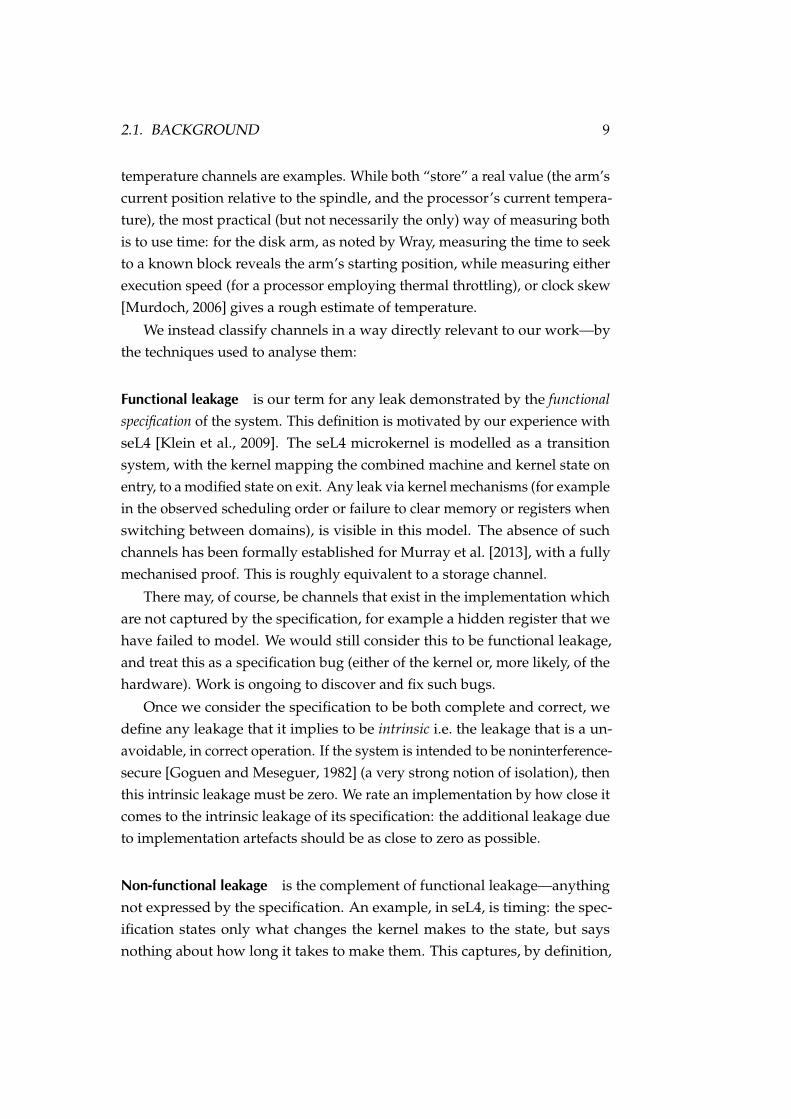
Functional leakage is our term for any leak demonstrated by the functionalspecification of the system. This definition is motivated by our experience withseL4 [Klein et al., 2009]. The seL4 microkernel is modelled as a transitionsystem, with the kernel mapping the combined machine and kernel state onentry, to a modified state on exit. Any leak via kernel mechanisms (for examplein the observed scheduling order or failure to clear memory or registers whenswitching between domains), is visible in this model. The absence of suchchannels has been formally established for Murray et al. [2013], with a fullymechanised proof. This is roughly equivalent to a storage channel.
There may, of course, be channels that exist in the implementation whichare not captured by the specification, for example a hidden register that wehave failed to model. We would still consider this to be functional leakage,and treat this as a specification bug (either of the kernel or, more likely, of thehardware). Work is ongoing to discover and fix such bugs.
Once we consider the specification to be both complete and correct, wedefine any leakage that it implies to be intrinsic i.e. the leakage that is a un-avoidable, in correct operation. If the system is intended to be noninterference-secure [Goguen and Meseguer, 1982] (a very strong notion of isolation), thenthis intrinsic leakage must be zero. We rate an implementation by how close itcomes to the intrinsic leakage of its specification: the additional leakage dueto implementation artefacts should be as close to zero as possible.
Non-functional leakage is the complement of functional leakage—anythingnot expressed by the specification. An example, in seL4, is timing: the spec-ification states only what changes the kernel makes to the state, but saysnothing about how long it takes to make them. This captures, by definition,

10 CHAPTER 2. COVERT AND SIDE CHANNELS
1 i n t2 strcmp ( const char ∗p1 , const char ∗p2 ) {3 r e g i s t e r const unsigned char ∗ s1 =4 ( const unsigned char ∗ ) p1 ;5 r e g i s t e r const unsigned char ∗ s2 =6 ( const unsigned char ∗ ) p2 ;7 unsigned reg_char c1 , c2 ;89 do {
10 c1 = ( unsigned char ) ∗ s1 ++;11 c2 = ( unsigned char ) ∗ s2 ++;12 i f ( c1 == ’ \0 ’ ) return c1 − c2 ;13 } while ( c1 == c2 ) ;1415 return c1 − c2 ;16 }
Figure 2.1: strcmp, from GNU glibc 2.9 (edited for readability).
all remaining sources of leakage, but our classification is context dependent.Time could be incorporated into the specification, as could any number ofphysical variables (temperature, for example). There are two reasons to avoidthis: First, the specification would be more complex, and we have no goodreason to suppose that we could complete a formal proof equivalent to that forthe functional specification (even if we had a specification of the hardware’sbehaviour); Second, the question, by its very nature, is open ended. Thehistory of research into side channels in particular is one of the progressivediscovery of more and more leaks not covered by existing models. There musttherefore be a category for vulnerabilities that we haven’t found yet.
Any classification of channels is likely to be to some extent arbitrary, andmoreover to reflect the bias of the classifier. We settle on the functional/non-functional distinction as it matches our verification approach, although weshortly refine it into the notions of intrinsic and extrinsic leakage, reflecting thedistinction between leakage implied by a specification, and that added by animplementation.

2.2. THE STRCMP CHANNEL 11
2.2 The strcmp Channel
To illustrate the problem, we analyse a timing channel in common implemen-tations of the C library’s strcmp (string compare) routine. We use this exampleto illustrate our notions of vulnerability and channel capacity, and also tomotivate our threat model: the guessing attack.
Figure 2.1 is typical, from GNU glibc version 2.9 (edited for readability).The comparison is performed by the loop at lines 9–13. This steps through thestrings in parallel (lines 10 & 11), until either the first ends (line 12, stringsare null terminated), or a mismatch is found (line 13). If the second stringis shorter, the loop terminates when its null terminator fails to match thecorresponding character in the first. The number of iterations, and thusexecution time, increases with the number of successful matches: the commonprefix length of the two strings.
An appropriate specification, expressed in Higher-Order Logic1 (HOL),is as a function from a pair of strings to a truth value, abstracting from thedetails of the implementation:
strcmp :: string× string→ bool
strcmp (s1, s2) ≡ (s1 = s2)(2.1)
If an attacker observes the execution time sufficiently closely, then he orshe learns much more than this simple specification indicates. The imple-mentation leaks more than the specification allows (the intrinsic leakage)—thenon-functional leakage in this example is substantial. Defining and measuringthis occupies the remainder of the chapter.
A Guessing Attack on strcmp
Imagine that our attacker is trying to guess a password by repeatedly invokinga password checker that uses strcmp. Usually, a guessing attack is expensive:exponential in the length of the password. We will see, however, that with theaddition of side-channel leakage, this becomes linear.
We begin by calculating the vulnerability given only the intrinsic leakageimplied by Equation 2.1.
1HOL is a formal logic for mathematical specification and proof. We make heavyuse of HOL in later chapters, where we mechanically verify leakage properties. Forthe moment, it is sufficient to consider this specification as an implementation in afunctional language, such as Haskell or ML.

12 CHAPTER 2. COVERT AND SIDE CHANNELS
2.3 Leakage with a Uniform Prior
Assume, for now, that all secrets are equally likely (perhaps generated uni-formly at random), and that the attacker knows the precise execution time.This is the simplest case, and we relax both assumptions shortly.
Suppose that the attacker supplies a string of its choice (a guess), whichthe system compares against its secret, answering yes (for a match) or no (fora mismatch). Let the secret consist of n characters, drawn from an alphabet ofm symbols, givingmn possibilities. Assume that this is known to the attacker.If the secret is chosen uniformly, the attacker has no reason to suspect thatone secret is more likely than another, and may as well guess in any order.After each guess, either the secret is found (the system answered yes), or theattacker eliminates a possibility.
As all remaining secrets are equally likely, the chance of guessing correctlyat each step is one over the number of possibilities remaining: The chance thatthe next guess is correct, having made k incorrect guesses, is
V0(k) =1
mn − k(2.2)
The subscript 0 indicates that this is the probability of compromise givenno additional information. This gives an obvious, fundamental measure ofvulnerability:
Definition 1 (One-Guess Vulnerability): For a system subject to guessing,the one-guess vulnerability, V0, is the chance that an optimal (computationallyunbounded) attacker can compromise it in a single attempt, given no extrainformation.
This has the benefit of being succinct, easily stated, and obviously applica-ble. The downside, as we’ll see, is that it is generally impractical to calculate.We thus focus on efficiently approximating, or bounding, V0.
Any definition of vulnerability is, implicitly or explicitly, made with refer-ence to a threat model—ours is the guessing attack. This may appear limiting,but it’s not. The class of systems vulnerable to guessing is very broad: Wecan include any system that authenticates using a secret. We can also includemost applications of cryptography. A protocol for authenticity (e.g. a digitalsignature) is subject to guessing in exactly the same manner as a password(keep guessing until the signature matches). A guessing attack against a confi-dentiality protocol (e.g. message encryption) is also simple, if the ciphertext

2.3. LEAKAGE WITH A UNIFORM PRIOR 13
133
132
13
1
0 3 6 9 12 15 18 21 24 27
V0
k
Figure 2.2: Vulnerability (V0) vs. number of guesses (k), for strcmp with noside channel, wherem = 3, n = 3.
is known. The attacker can conduct an offline guessing attack (in contrastto the online attack against the password checker), by trying keys one at atime, until the message is decrypted. The attacker has a nonzero (thoughvanishingly small) chance of guessing correctly on the first attempt. We doneed to assume that the attacker is able to recognise valid plaintext. Thus,one-time-pad encryption is not vulnerable to guessing [Shannon, 1948].
Returning to our example, Figure 2.2 plots V0 given only intrinsic leakage,for m = 3 and n = 3: secrets of length 3 drawn from an alphabet of 3symbols. We see that vulnerability initially rises very slowly (the verticalscale is logarithmic, to better discriminate smaller values), and reaches 1(compromise) after 26 guesses. At this point, the attacker knows that there isonly one possible secret, of the initial 33 = 27.
How does adding a side channel affect V0? That is, how does the leakageadded by the implementation of Figure 2.1 compare to the intrinsic leakage ofFigure 2.2? Clearly, V0(0) will not change, as leakage is only observed afterguessing. We only deviate after the first guess, and if the attacker is optimal,vulnerability only increases (on average) given more information. Note thatthe curves must meet again after mn − 1 guesses, as with only one secret

14 CHAPTER 2. COVERT AND SIDE CHANNELS
remaining in either case, the attacker will guess correctly with probability 1.
How does the curve behave between k = 0 and k = mn − 1? Recallthat the we leak the execution time of the strcmp routine, which exposesthe common prefix length of the guess and the secret. Take the place of theattacker. Knowing the prefix length, we attack the positions individually: Tofind the first, we generatem strings of length n, differing in the first position,and pass these to the system. m − 1 of these will fail to match in the firstposition, and thus the loop will execute once (as it is post-checked). One,however, will match, and we will see at least 2 iterations. The string givingthe longest runtime thus has the correct character in the first position (andpossibly more). Repeat for the remaining characters: Once i positions areknown, we find position i (strings are zero indexed), by setting 0 . . . i− 1 totheir known values, and varying i, looking again for the greatest responsetime.
The Vulnerability Model
Given this strategy, we can calculate V0(k). Every incorrect guess now elimi-nates not just one, but a set of secrets: when 0 . . . i− 1 are known (thus we’reguessing position i), if we see only i+ 1 iterations, our guess for i was wrong.This eliminates not only our guess, but any that match it in its first i positions(mismatches in 0 . . . i− 1 have already been ruled out, by induction). If we seei+ 2 or more iterations however, we have the correct character in position iand eliminate all other possibilities.
With leakage, plotting V0 against time is much more complicated. Fig-ure 2.3 shows all possible traces form = 3,n = 3 (in red), with the number ofguesses along the horizontal axis, and the current value of V0 on the vertical.A single trace begins at {0, 1/27}, at the bottom-left, and on each guess movesone step right and some number upward (as it may guess several positions atonce). The shaded circles show the likelihood of reaching a state, normalisedby column. Thus, a circle at {k, v} gives P(v|k): the conditional probability ofseeing vulnerability v after k guesses. The vertical axis is logarithmic, as is thevertex shading. The no-leakage trace is included (in blue), for comparison.
The increase in vulnerability is obvious: all traces reach V0 = 1 by the6th guess, whereas the original attack took until the 26th. However, this onlycompares the worst-case for each attack. How do they compare on average?

2.3. LEAKAGE WITH A UNIFORM PRIOR 15
133
132
13
1
0 1 2 3 4 5 6 7
V0
k
No leakageWith leakage
P(V0|k)
Figure 2.3: strcmp attack traces with leakage for m = 3, n = 3, showingvulnerability (V0) vs. number of guesses (k), and log2 P(V0|k) at each vertex.Includes the no-leakage trace in blue for comparison
166
165
164
162
16
1
0 10 20 30
V0
k
P(V0|k)10th and 90th Percentiles
Median
Figure 2.4: strcmp attack traces form = 6, n = 6, showing vulnerability (V0)vs. number of guesses (k), and log2 P(V0|k) at each vertex. Includes the 10th,50th and 90th percentiles for P(V0|k).

16 CHAPTER 2. COVERT AND SIDE CHANNELS
Increasing tom = 6 and n = 6 gives Figure 2.4. Here we drop the traces,leaving only vertices, for clarity. They follow the same pattern as in Figure 2.3.We also drop the no-leakage curve, as it never rises high enough to be visible:it now takes until k = 66 − 1 = 46, 655 to reach V0 = 1 without leakage, withall leakage traces terminating by k = 30.
Including the median (blue) and the 10th and 90th percentiles gives afeeling for the distribution of traces: 90% lie above the 10th percentile (therightmost red curve) at any given k. Note that a trace may cross a percentile,and that the percentile itself does not (necessarily) represent a trace. We seethat 90% of all traces find the secret in no more than 15 guesses, with halftaking less than 9. The distribution is thus clustered to the left, with a longright-hand tail. The worst-case length (the defender’s best case) is thus anoverestimate and a poor guide to likely vulnerability. The best-case is likewisea dramatic underestimate: 1 guess.
How can we quantify this increase in vulnerability? Figure 2.4 contains allthe information we need, certainly, but we want a summary measure. Thereare two reasons: Firstly, the full distribution is a clumsy way to describe thesystem; Secondly, and more importantly, we can’t generate these figures foranything more than toy examples.
As a measure, V0 isn’t good enough on its own as it only refers to thecurrent state and doesn’t take into account any future leakage. ConsiderFigure 2.4 again, and imagine that we are on a trace similar to the (blue)median. Suppose we reach V0 = 1/64, after 6 guesses. Taking only V0 intoaccount (given our uniform search space), there are 64 = 1296 equally-likelysecrets which, given no extra information, would take on average 648 furtherguesses. From the figure however, we expect to get the secret correct in only 3additional guesses! Using only V0, we would assign this outcome a probabilityof only 3/1296. We thus need to take future leakage into account.
We must note that we are making a qualitative judgement regarding whatwe want in a security measure. Our strawman (the expected number ofguesses remaining), exemplifies one particular style of measure: expected timeto compromise. This example, where we ignore future interaction with thesystem, and let the attacker perform, say, an offline brute-force attack, isknown as the guessing entropy[Massey, 1994], and is defined as:∑
i
iP(xi)

2.3. LEAKAGE WITH A UNIFORM PRIOR 17
where the xi are the list of possible secrets, arranged in order of decreasinglikelihood.
These measures are widely used, and intuitively reasonable, in the fieldof cryptography, where the primary concern is often with a well-resourcedattacker performing an offline cryptanalysis (essentially a sophisticated guess-ing attack) against captured ciphertext. Here, the argument is in terms of thecost of the attack, relative to the value of the secret, and is quantified by thework factor of a cryptosystem.
The difficulty in applying such a measure here is that it depends criticallyon the assumption of uniformity. For a cryptographic key or a nonce2, a greatdeal of effort is made to ensure the uniformity and unpredictability of thesecret, and thus this assumption holds. In the case of a password, or theleakage of sensitive control-flow information, this assumption does not hold.Passwords in particular are well recognised, ([Dell’Amico et al., 2010; Maloneand Maher, 2012]), to be non-uniformly distributed, with some astonishinglycommon. In this case, knowing the expected time to compromise gives uslittle confidence in the security of the system.
In the extreme, if we have one secret of probability 0.99, and 10100 secretsof probability 10−102, the expected time to compromise is roughly 0.99× 1 +
0.01× 10100/2 ≈ 1098, an enormous number. The probability of compromisein a single guess however, is 99%! We cannot assume uniformity on secrets,and we must judge a system like this to be insecure. We therefore use expectedchance of compromise, rather than expected time to compromise. The one-guessvulnerability is a simple example of such a measure. The advantage is thatwe avoid the above problem; The disadvantage is these measures are oftendifficult to calculate, as already established for strcmp.
We now show that we can, with appropriate care, bound chance of compro-mise, given only an average security measure. This allows us to combine thesimplicity of time-to-compromise, with the rigour of chance-of-compromise.
This problem, the disconnect between chance-of-compromise and time-to-compromise, was recognised by Smith [2009], specifically between theShannon entropy and the min entropy. The Shannon entropy is a summarymeasure that we will introduce shortly, while the min entropy is a worst-casemeasure, and is equivalent to V0. There has been a great deal of interest in
2A nonce is a randomly-selected single-use token. Its most important property isthat it should be unpredictable to an attacker, and is thus usually selected at random.

18 CHAPTER 2. COVERT AND SIDE CHANNELS
min entropy as a vulnerability measure [Espinoza and Smith, 2013], leading tothe recent work of Alvim et al. [2012], showing that when generalised (to gainfunctions), it subsumes most other measures. Our contribution is to show thatwhile the worst case is indeed as established, this only occurs for pathologicaldistributions, and that if care is taken, Shannon entropy can be used safely.
Multiple Guesses
To incorporate leakage across multiple steps, we extend our measure fromone guess (and no observations) to many:
Definition 2 (k-Guess Vulnerability): The system is compromised once V0 =
1, i.e. the attacker knows the secret, and is certain to guess correctly on its nextattempt. The k-guess vulnerability, or Vk, is the probability that the systemwill be compromised given at most k guesses. That is, it is the probability thatV0 = 1 after k guesses (and k− 1 observations, for 0 < k).
For any k, Vk+1 is at least as high as Vk: An extra guess gives the attackeranother attempt, which succeeds with non-negative probability. We apply themeasure by setting k appropriately: If we’re analysing a password checkerthat allows only three tries before disabling logins, then setting k to 3 givesthe probability of compromise. In a cryptographic setting, k might indicatethe attacker’s estimated computational power: If we’re confident that theattacker can’t process more that, say, 109 keys in a reasonable timeframe thenV109 again gives the overall chance of compromise.
Figure 2.5 shows vulnerability against time (number of guesses) for them = 6,n = 6 example. This plot is generated from the same data as Figure 2.4.Vk is plotted in orange, and rises to one by about the 10th guess. Let V0(k) bethe expected vulnerability after k guesses, assuming that the secret hasn’t beenguessed yet. From this, we can reconstruct Vk as:
Vk = V0(0) +(1 − V0(0)
)×[V0(1) +
(1 − V0(1)
)× . . .
]That is, the probability that we guess by the kth attempt is the probability thatwe guess on the first attempt, plus the probability that we don’t multiplied bythe probability that we guess correctly somewhere between attempt 1 and k,given that we guessed wrong at 0.
We can thus translate between the two measures, and will calculate usingV0(k) from now on. We see the benefit by considering the remaining curves

2.3. LEAKAGE WITH A UNIFORM PRIOR 19
1
6
62
64
65
66
0 3 6 9 12 15 18 21 24 27 300
0.25
0.75
1
1/V V
k
66−k/3
E(1/V0(k))V0(k)Vk
Figure 2.5: k-guess vulnerability (Vk) vs. k, for m = 6,n = 6, togetherwith expected one-guess vulnerability (V0(k)). Also shown are the expecteduncertainty set size (E(1/V0(k))), and the linear trend assuming 1 position isfound every 3 guesses, showing roughly log-linear behaviour.
in Figure 2.4. V0(k) is plotted in green, and as we see it always lies below Vk:This is as we expect, as it considers only the probability of terminating onguess k, and ignores the probability of terminating earlier.
Recall from Equation 2.2 that V0, the one-guess vulnerability, is inverselyproportional to the number of possible secrets remaining, as they are uniformlydistributed. Thus, the reciprocal of V0 in any state is the size of this uncertaintyset. We plot the expectation of this value in red, that is, the size of the expecteduncertainty set. This shows how many secrets remain, on average, after kguesses. Rather than directly measuring security, as V0 does, this quantifiesthe amount of work remaining for the attacker—a time-to-compromise measure.This curve shows us something interesting: Up to 15 guesses (at which pointthe system is almost totally compromised), the logarithm of the uncertainty-set size decreases more-or-less linearly (note that the left-hand vertical scale islogarithmic).
The blue line gives a lower bound on this size, and hence an upper boundon leakage. Here we see that the size of the uncertainty set decreases by a

20 CHAPTER 2. COVERT AND SIDE CHANNELS
factor of 6, approximately every 3 guesses. This is equivalent to saying thatthe attacker guesses one position per 3 attempts, which is what we expectgiven that there are 6 possibilities per position. This tells us that vulnerabilityis approximately log-linear: the ratio of the set sizes remains roughly constantfor a given interval. This suggests a logarithmic definition of leakage:
Definition 3 (Uncertainty Set): For a leakage profile in which the set ofpossible secrets is always uniformly likely, let Su be this uncertainty set: the setof secrets of nonzero probability. The uncertainty set measure is then the sizeof this set:
Vu = ‖Su‖ (2.3)
Leakage is the ratio of vulnerability between two states:
Lu =‖Su‖‖S′u‖
(2.4)
Note that, if the probability is uniform, V0 = 1/Vu, and the two measures areequivalent.
The power of this definition is that we have a single summary measureboth for vulnerability (Vu), and for leakage (Lu), that in our example allowsa fair approximation by a simple linear model. We will see shortly thatthis measure also remains useful when we abandon first the assumptionof uniformity (Section 2.4), and then of complete knowledge (Section 2.6).Generalising leads us eventually to Shannon entropy (Equation 2.10).
Limitations
Before we continue, we need to recognise the limitations of this model. Inderiving this measure from Vu, we have thrown away information. Recallthat we started by noting that 1/V0 = Vu, thanks to uniformity. From this, wehypothesised that 1/E(Vu) might be a useful approximation to Vn = E(1/Vu).Note that, in general, E(1/X) 6= 1/E(X): the expectation does not commutewith the reciprocal. The two measures are plotted together in Figure 2.6. Wesee that, while our estimated vulnerability curve (red) has roughly the sameshape as the true curve (green), it is offset to the right by about 12 guesses.That is, it predicts that a given degree of compromise will occur 12 guesseslater than it really does, and thus underestimates vulnerability.
Why is this such an underestimate? We’d like to take advantage of thelinear relationship we discovered in Figure 2.5, which would give us a single
2.3. LEAKAGE WITH A UNIFORM PRIOR 21
0
0.2
0.4
0.6
0.8
1
0 5 10 15 20 25 30k
1/E(Vu)V0(k)
Figure 2.6: Expected vulnerability, and vulnerability estimated from expecteduncertainty set size, showing the similar shape of the curves.
number (the slope), as the constant leakage rate of the system. The fact thatthe two curves have a similar shape is suggestive, and if we were to shift ourestimate left by 12 guesses, we would have a reasonable approximation to thetrue vulnerability (for this system, at least). Is there any way in which this istheoretically justifiable? Luckily enough, there is.
As noted, a summary measure throws away information. In particular,there may be many distributions with a given E(V0), but for these, 1/E(1/V0)
will generally differ. Recall that in calculating V0(k), we are working with adistribution on the states of the system after k guesses. The only quantity thatmatters for the calculation of V0 is the size of the uncertainty set, which rangesfrom 1 tomn.
We can still bound the range of values that the true vulnerability, E(V0),may take. The question is: what is the largest possible value of E(V0) for anydistribution for which 1/E(1/V0)) is known? The answer is relatively simpleas, while the function 1/x is not linear, it is (anti-)monotonic.

22 CHAPTER 2. COVERT AND SIDE CHANNELS
Pessimistic Correction
Lemma 1 (Maximising the Reciprocal Expectation): Let X be a randomvariable, ranging over the integers [1,n]. For any fixed y, over all distributionswhere E(X) = y, E(1/X) is maximised when all probability mass is assignedeither to 1 or to n.
Proof. See Appendix A
Lemma 2 (Pessimistic Correction of Expected Uncertainty Set): For a secretof length n, drawn uniformly from an alphabet of sizem, the greatest possibleexpected vulnerability, E(V0), over all distributions where E(1/V0) is heldconstant, is:
1 −1mn
−E(1/V0)
mn(2.5)
Proof. First, we use the fact that V0 = 1/‖Su‖ to instead look for the maximalvalue of E(1/‖Su‖), where E(‖Su‖) is known. By Lemma 1, this must beattained by a distribution that assigns nonzero probabilities only to ‖Su‖ = 1,and ‖Su‖ = mn. There is only one such distribution, satisfying the linearequations:
P(‖Su‖ = 1) +mnP(‖Su‖ = mn) = E(‖Su‖)
P(‖Su‖ = 1) + P(‖Su‖ = mn) = 1
solving gives:
P(‖Su‖ = 1) =mn − E(‖Su‖)
mn − 1
P(‖Su‖ = mn) =E(‖Su‖) − 1mn − 1
whence,
E(1/‖Su‖) = P(‖Su‖ = 1) +P(‖Su‖ = mn)
mn
=mn − E(‖Su‖)
mn − 1+E(‖Su‖) − 1mn(mn − 1)
= 1 −1mn
−E(‖Su‖)mn

2.3. LEAKAGE WITH A UNIFORM PRIOR 23
0
0.2
0.4
0.6
0.8
1
0 5 10 15 20 25 30k
V0(k)Pessimistic correction of E(1/|Su|)
Pessimistic correction of linear model
Figure 2.7: Pessimistic correction of the uncertainty-set measure.
We use Equation 2.5 to transform the expected uncertainty set size inFigure 2.5 to a safe upper bound on vulnerability, as plotted in Figure 2.7. Wesee that while our new bound is pessimistic, it is safe. Moreover, we can applyit to the linear model of Figure 2.5 (1 position every 3 guesses), to get a verysimilar, and also safe upper bound.
Summary We have established that in the case of a uniform distribution onsecrets, leaking the common prefix length dramatically shortens a successfulguessing attack against strcmp (Figure 2.2 vs. Figure 2.3). While the number ofoptimal attack traces is large, they are unevenly distributed, with short tracesbeing most likely, and a long tail (Figure 2.4). While the expected vulnerabilitygrows rapidly and non-linearly, we see that during most of the attack, theattacker’s uncertainty set shrinks geometrically: log|Su| is approximately linear,with a slope of log 6/3, corresponding to our intuitive model of one positionguessed on average, per 3 attempts.
From a log-linear model of leakage, we reconstruct a safe bound on ex-pected one-guess vulnerability (V0), by establishing how far the true set sizecan deviate from its expectation. We are thus able to use a model that matchesthe observed behaviour of the system (linear leakage) but that is nonetheless

24 CHAPTER 2. COVERT AND SIDE CHANNELS
safe. We model the system using a single parameter: the leakage rate, whileretaining a safe bound on vulnerability.
2.4 Leakage with a Nonuniform Prior
We have so far assumed that secrets are chosen evenly at random—that theattacker’s prior distribution is uniform. Imagine instead that the secrets arechosen according to some distribution PS. How does this change our results?There are two reasons to relax this assumption: First, we may be dealingwith secrets that really are non-uniform (passwords, or the output of a weakrandom number generator); Second, as the attacker makes observations, itwill begin to consider certain secrets to be more likely than others (those thatare more likely to produce the output that it’s seen). Thus, after some numberof observations, the attacker’s beliefs form a non-uniform distribution, andwe’d like to quantify how much more vulnerable the system has become.
Let us return first to the one-guess vulnerability, V0 (Definition 1). Herethere is little change. Where previously it didn’t matter which secret (of thosewith nonzero probability) the attacker guessed, an optimal attacker will pickthe most likely. Thus in general,
V0 = maxsPS(s) (2.6)
This formula is still valid in the uniform case, albeit trivial.What about our uncertainty set measure? We’d like to retain the simple
linear leakage model, but is this possible? First, we need to establish theoptimal attack strategy. Under uniformity, all guesses were equally good,but that is no longer true. The attacker obviously maximises its chance ofguessing correctly straight away, and hence V0, if it chooses a secret thatmaximises PS(s) i.e. one of those that are most likely (there may be more thanone). However, it is not obvious that doing so maximises its chances for a laterguess, if the first one fails. We could imagine a situation where the top twosecrets have almost, but not quite, identical probabilities. It might also be thecase that if we guess the less likely of the two, the side-channel informationwill reveal the correct value to us, even if our guess was incorrect. In thiscontrived example, we would maximise V0 by guessing the first secret (themost likely), but we would maximise Vn for any 1 6 n by guessing the second.We could not do both. In this case, we could be optimal with respect to V0 or

2.4. LEAKAGE WITH A NONUNIFORM PRIOR 25
to Vn, but not both. We must therefore further analyse the leakage that ourstrcmp example actually produces, to establish the optimal attack.
Detailed Analysis of an Optimal Attack
We first note a standard result in probability:
Lemma 3: Any joint distribution P(X1, . . . ,Xn) over a set of n random vari-ables (not necessarily independent), can be expressed in terms of incrementalconditional distributions:
P(x1, . . . , xn) = P(xn|xn−1, . . . , x1)P(xn−1|xn−2, . . . , x1) . . .P(x1)
=∏i
P(xi|xi−1, . . . , xn) (2.7)
Proof. This is a standard result, and follows from the definition of conditionalprobability.
Let si be the character in position i in the putative secret, s. The probabilitythat the secret is in fact s is then the joint probability that all positions arecorrect, or P(s1, . . . , sn). By Lemma 3, we may rewrite this as the product ofthe conditional probabilities P(sk|sk−1, . . . , s1)—the probability that the kth
position is sk, given that the first k− 1 positions have values s1 through sk−1.
Consider an attack that has exposed j − 1 positions: s1 through sj−1 arenow known. If the attacker wants to maximise its chance of a successful guess,to optimise V0, it needs to choose the most likely values for the remainingpositions, given what it now knows — it needs to choose sj through sn tomaximise P(sn, . . . , sj|sj−1, . . . , s1). A computationally unbounded attackermust be assumed to be capable of finding such an assignment.
Suppose, alternatively, that the attacker wants to maximise its chance ofguessing correctly on the next try, assuming that the current guess is incorrect(a reasonable assumption in the early stages of an attack). In this case, theattacker is seeking to maximise the leakage due to the next guess, or V0(k +
1) − V0(k). Considering only position j, there are two possibilities, if we fail toguess correctly: either sj was wrong, in which case we strike it from our list ofpossibilities and keep trying at position j, or it was correct, in which case weeliminate every other possibility and continue guessing at some later position(not necessarily j+ 1). What is the effect on V0 in each of these cases?

26 CHAPTER 2. COVERT AND SIDE CHANNELS
To answer this, we recall another standard result, Bayes’ theorem:
P(h|e) =P(e|h)P(h)
P(e)(2.8)
This result is the foundation of statistical inference: it formalises the processof updating a statistical model, given new evidence. To see this, it is helpfulto rewrite is in this form:
P(h|e) =P(e|h)
P(e)× P(h) (2.9)
This is a recipe for converting P(h), the probability that hypothesis h holdsgiven no additional evidence (the prior probability of h), into P(h|e), the prob-ability that h holds, once we have observed the evidence, e (the posteriorprobability of h). The important point is that this is exactly what the attacker isdoing: It begins with some idea, or belief, of how likely each secret is (initiallywe assumed this to be the uniform distribution, which assumption we nowrelax), and given the evidence that it observes (the intrinsic leakage—thematch/mismatch response, and the side-channel leakage—the common prefixlength), updates its belief, making some secrets less likely, and others more.Equation 2.9 tells us how an optimal attacker does this: the prior probability ofa secret, P(s), is multiplied by the probability of seeing o, if the secret were s,or P(o|s) (the consequent probability of o), divided by the probability of seeingo in any case, or P(o). This factor is the evidence ratio.
We apply Equation 2.9 to calculate the posterior probabilities for a correct,and an incorrect guess at position j. Suppose first that our guess was wrong:that is, we observed a common prefix length (cpl) of j− 1. The probability ofobserving this, if the jth character really were sj is zero:
P(cpl = j− 1|sj, . . . , s1) = 0
Thus, the evidence ratio is zero, and so is the posterior probability that sj iscorrect, knowing that the first j − 1 characters are correct, but having observed acommon prefix length of only j− 1:
P(sj|cpl = j− 1, sj−1, . . . , s1) = 0
What about the other possibilities, the other characters that we might haveguessed? For each of these, say s′j, the probability of the evidence is one. That

2.4. LEAKAGE WITH A NONUNIFORM PRIOR 27
is, if the correct value is s′j but we guessed sj, then the common prefix lengthmust be j− 1:
P(cpl = j− 1|s′j, . . . , s1) = 1
This time, we need to evaluate the denominator—the prior probability of theevidence. This is the probability of seeing a prefix length of j− 1, given thatwe guessed sj, without knowing whether or not our guess is correct. Here we usethe decomposition introduced in Lemma 3. Given that s1 through sj−1 arecorrect, the probability that the prefix length is only j − 1, is the probabilitythat the position sj is wrong, given that the first j− 1 positions are correct:
P(cpl = j− 1|sj, . . . , s1) = 1 − P(sj|sj−1, . . . , s1)
Thus, for any secret that matches s1 through sj−1 and sj, the posterior prob-ability is zero–it’s been ruled out (any mismatches between s1 and sj−1
have already been ruled out by induction). Any secret that matches s1
through sj−1 but doesn’t match sj has its probability increased by a factor of1/(1 − P(sj|sj−1, . . . , s1)). Note that any secret whose probability is alreadyzero remains ruled out. The effect is thus to rule out a set of secrets, anduniformly scale up the probabilities of all the remaining possibilities, suchthat the sum is still one.
What if we guessed correctly? In this case the probability of every secretthat doesn’t match at sj should go to zero, and we see that this is exactly whatBayes’ rule gives us. The probability of seeing a prefix length of j or more,were the correct value anything other that sj is zero, and thus:
P(cpl > j|s′j, . . . , s1) = 0
From this we see that the posterior probability does indeed go to zero. On thecontrary, if the correct value were sj, we must see a prefix length of j or more:
P(cpl > j|sj, . . . , s1) = 1
We must again consider the probability of the evidence, which is now theprobability that our guess is correct, or:
P(cpl > j|sj, . . . , s1) = P(sj|sj−1, . . . , s1)
and thus
P(sj|cpl > j, sj−1, . . . , s1) =1
P(sj|sj−1, . . . , s1)× P(sj|sj−1, . . . , s1) = 1

28 CHAPTER 2. COVERT AND SIDE CHANNELS
c
1��a
1/3
ss1/3��
1/3
++a1/3
{{1/3��
1/3
##
b1/3
{{1/3��
1/3
##
c1/3
{{1/3��
1/3
##a b c a b c a b c
1/9 1/9 1/9 1/9 1/9 1/9 1/9 1/9 1/9
Figure 2.8: An attack state (m = 3,n = 4) represented as a tree. Every pathfrom the root is a possible secret. The prefix ‘ca’ has been established. Theedge from sj−1 to sj is labelled with P(sj|sj−1, . . . , s1). The leaves are labelledwith the probability of the path that leads to them, or P(sj, . . . , s1)
c
1��a
0
ss1/2��
1/2
++a1/3
{{1/3��
1/3
##
b1/3
{{1/3��
1/3
##
c1/3
{{1/3��
1/3
##a b c a b c a b c
0 0 0 1/6 1/6 1/6 1/6 1/6 1/6
Figure 2.9: The attack in Figure 2.8 after guessing ‘caaa’ and seeing a pre-fix length of 2. The left subtree has been eliminated, and the conditionalprobabilities of the others adjusted, changing the probabilities at the leaves.
So in this case, all secrets that don’t match at sj are ruled out, while all thosethat do are scaled up by a factor of 1/P(sj|sj−1, . . . , s1).
This is not the only inference we can make, however. It’s always possiblethat we have guessed more than one additional character correctly: cpl couldbe anywhere from j to n. In this case, we eliminate even more possibilities—those that don’t match at some point between j and cpl, inclusive. To visualisethis, it is useful to view the space of secrets as a tree. Figure 2.8 illustratesthe attacker’s distribution over secrets, partitioned according to Equation 2.7,withm = 3 and n = 4. The attacker knows that the first two characters are ‘c’

2.4. LEAKAGE WITH A NONUNIFORM PRIOR 29
c
1��a
1
ow0��
0
++a0
{{1/2��
1/2
##
b1/3
{{1/3��
1/3
##
c1/3
{{1/3��
1/3
##a b c a b c a b c
0 1/2 1/2 0 0 0 0 0 0
Figure 2.10: The attack in Figure 2.8 after guessing ‘caaa’ and seeing a prefixlength of 3. The middle and right subtrees have been eliminated, as has thesubtree rooted at ‘caaa’.
c
1��a
1
ow0��
0
++a0
{{1��
0
##
b1/3
{{1/3��
1/3
##
c1/3
{{1/3��
1/3
##a b c a b c a b c
0 1 0 0 0 0 0 0 0
Figure 2.11: The attack in Figure 2.8 after guessing correctly that position jis ‘a’, and that position j+ 1 is ‘b’. The middle and right subtrees have beeneliminated, as have ‘a’ and ‘c’ in the final row.
and ‘a’, and is attempting to guess the third. In this example, the distributionof secrets is initially uniform, and is recorded in the final row of the figure,under the leaves. The probability at a leaf is the probability of the secret speltout by following the path from the root. For example, the probability thatthe secret is ‘cacb’ is 1/9. This is the product of the probabilities attached tothe edges along the path, in this case P(c) × P(a|c) × P(c|ac) × P(b|cac), or1× 1× 1/3× 1/3.
Observing the response lets us update the conditional probabilities alongthe edges between the last known position and the observed prefix length.For example, Figure 2.9 shows the result of guessing incorrectly at position

30 CHAPTER 2. COVERT AND SIDE CHANNELS
3. Here, the subtree rooted at the first incorrect character, s3, is eliminatedand the conditional probabilities leading to the others are scaled accordingly.Note that only the conditional probability for the guess we actually made isupdated: the conditional probabilities lower in the eliminated subtree are notchanged, but the zero at the root ensures that any path through that subtreehas probability zero.
Figure 2.10 shows the result of a correct guess against position 3, whichfails at position 4, corresponding to an observed prefix length of 3. Here allother subtrees at depth 3 are eliminated, as is the subtree at depth 4 rootedat our first incorrectly guessed position. Finally, Figure 2.11 shows whathappens when more than one position is guessed at once: all other subtreesare eliminated at every level down to the first mismatch. In this case, we haveguessed the entire secret correctly, but if there were further levels, the subtreecorresponding to our hypothetical mismatch at level 5 would be eliminated,as for Figure 2.10.
Note that in every case, we eliminate some number of subtrees and scalethe rest uniformly. Importantly, this means that if the secrets are ordered byprobability then this does not change, we simply knock holes as we go. Thismakes simulating the attack tractable.
So far we have considered only intrinsic leakage. The effect of adding side-channel observations is to change the relative weights of the branches that areleft un-pruned, and thus the bottom-row probabilities for complete secrets.We have left this out of our discussion so far, but it does not effect the basicpattern of pruning a branching model that we have established. It is taken intoaccount in the following section, where we simulate a statistically-optimalattacker.
Updating the Leakage Model
This attack strategy is too complicated to analyse exactly, as we did in theuniform case, especially as it depends on the details of the prior distributionon secrets. To understand how it behaves, we instead run an exhaustivesimulation. We attack every possible secret with two strategies: one that picksthe most likely guess (maximising V0), and one that guesses to maximise theconditional probability at each branch (maximising leakage, or V0(k + 1) −V0(k)). To keep the simulation tractable, we assume that the distribution onsecrets is Markovian: the probabilities for position j+ 1 depend only on the

2.4. LEAKAGE WITH A NONUNIFORM PRIOR 31
0
4
12
16
0 5 10 15 20 25 300
0.25
0.75
1
H1(b) V
k
E(H1), nonuniformV0(k), nonuniform
E(H1), uniformV0(k), uniform
Figure 2.12: Comparison of one-guess vulnerability (V0) and expected entropy(H1) for a uniform, and a Markov prior. m = 6,n = 6.
character in position j. This is a reasonable model for the broad statisticalstructure of natural text, in particular passwords, which is of clear relevanceto this particular example [Dell’Amico et al., 2010].
The benefit to tractability is that the incremental probabilities all collapse:P(sj+1|sj, . . . , s0) is simply P(sj+1|sj)—every node in the tree has the samepattern of conditional probabilities among its branches. We compress theattacker’s model by only storing those branches that have been updated—anybranch that hasn’t yet changed is simply assumed to have its prior, Markovian,transition probability. To unify the treatment of the initial character (as there’sno previous character to transition from), we extend the alphabet with aspecial ‘start-of-word’ character, ·. Our table of transition probabilities wasgenerated from the file alice_29.txt of the Canterbury data-compressioncorpus [Arnold and Bell, 1997], representing the English text of Lewis Carroll’sAlice in Wonderland [Carroll, 1865].
Figure 2.12 shows the result of an exhaustive simulation of the m = 6,n =
6 case (the alphabet was restricted by taking themmost common characters,ordered by position-independent probability, and rescaling the transitionprobabilities). Also reproduced are the equivalent results in the uniform

32 CHAPTER 2. COVERT AND SIDE CHANNELS
case, from Figure 2.5. The expected vulnerability, V0(k), for the non-uniformcase is blue, while that for the uniform case is green. We see that the non-uniform vulnerability follows roughly the same path as the uniform case, butstarts at a higher value. This is expected, as in a non-uniform distribution,at least one secret must have greater-than-average probability. We see thatthe known prior is roughly equivalent to an additional 4 guesses’ worthof information. There was little or no difference between the two guessingstrategies: these results are for individually-maximised branch probabilities.This is an interesting result in its own right, and means that the attacker mayas well optimise locally (for just the next character).
The two additional curves in the figure (red and yellow) need a littlemore explanation. Rather than the expected uncertainty set size, as plottedin Figure 2.5, we here plot the Shannon entropy, or H1. This is a quantity offundamental importance in information theory—a measure of the ‘size’ ofa set, taking into account uneven likelihood amongst its members. For adistribution P, the Shannon entropy is defined as:
H1 = −∑x
P(x) log2 P(x) (2.10)
Here the logarithm is taken to base 2, giving an answer in bits. The entropyunder a different base differs only by a constant factor. Note that if thedistribution P is uniform i.e. P(x) = 1/|S|, then H1 = log2|S|. Thus, by plottingVu on a logarithmic scale, we actually snuck Shannon entropy in some timeago, under the guise of the uncertainty set. The red curve in Figure 2.12is thus identical to that in Figure 2.5. Importantly, the new yellow curve,giving the expected entropy vs. guess number for a non-uniform prior hasthe same slope, shifted down according to the difference in the initial entropy.This gives meaning to our log-linear leakage measure: saying that ‘set sizedrops by a factor of 6 every 3 guesses’ means that we are leaking (on average)log2 6 ≈ 2.58 bits every 3 guesses, or 0.86 bits per guess. Changing the priordistribution has not affected the rate of leakage, only the initial entropy, andour linear model is still valid.
There is an alternative definition of entropy that gives a worst-case, ratherthan an average-case summary: the min entropy. This measure depends on thegreatest probability in the distribution alone:
H∞ = − log2 maxxP(x) (2.11)

2.5. REEVALUATING SHANNON ENTROPY 33
Note the relation to Equation 2.6: the min entropy is simply the (negated)logarithm of the one-guess vulnerability for an optimal attacker. We compareleakage measures derived from these two definitions shortly.
Given that we have replaced the expected set size by the entropy, we mustask whether the pessimistic correction that allowed us to bound one-guessentropy still holds, and if not, with what we should replace it. As alreadynoted, Smith [2009] demonstrated that for some distributions, Shannon en-tropy is a very poor guide to one-guess vulnerability—the two may divergedramatically. This observation has lead to a strong move away from Shannonentropy in the literature, toward min entropy, as a safer measure.
Knowing that they diverge in some cases only establishes that entropy doesnot give us a universally applicable bound. However, if we can bound thisdivergence, we can show that Shannon entropy can be used as a safe securitymeasure. What we need to know is: How bad can the vulnerability be, if weknow the entropy? We derive this divergence exactly, as the subject of the nextsection.
2.5 Reevaluating Shannon Entropy
Figure 2.12 shows that the simple model of Figure 2.7 still holds. There wesaw that the size of the uncertainty set fell geometrically i.e. the logarithm felllinearly. We now see that the generalisation of the (log) uncertainty set size toa non-uniform distribution, the Shannon entropy, also shows a linear decrease(down to the point at which we reach a vulnerability of 0.5, at least). We thuscontinue to use a linear leakage model. Just as in Lemma 2 however, we needto take into account that we have only a summary measure of the distribution.There we knew the expected uncertainty set size, while here we know onlythe entropy of the distribution—there may be many distributions with a givenentropy, with different vulnerabilities. We thus need to establish the greatestpossible vulnerability given Shannon entropy.
The Divergence of Vulnerability and Shannon Entropy
Our key result is the following lemma, which tells us how to maximise vul-nerability while holding entropy constant. From this, we show that the vul-nerability increases (approximately) linearly, as entropy decreases.

34 CHAPTER 2. COVERT AND SIDE CHANNELS
Lemma 4 (Maximising V0 Given H1): Let
Q = {P : H1(P) = H}
be the set of distributions over the set X with Shannon entropy H. Let N = |X|.Fix n ∈ N and for each P ∈ Q, partition X (disjointly) as Y ∪ Z such that
∀y ∈ Y, z ∈ Z. y > z∧ |Y| = n
For all distributions P ∈ Q, P(Y) (the combined probability of all y ∈ Y) isbounded above by the curve
h(p) + p log2 n+ (1 − p) log2(N− n) (2.12)
where
h(p) = −p log2(p) − (1 − p) log2(1 − p) and 0 log2 0 = 0
Moreover, this bound is tight. For H > log2|Y|, it is reached by a distribu-tion of the form
P(x) =
P(Y)/‖Y‖ x ∈ Y
(1 − P(Y))/‖Z‖ x ∈ Z
If H < log2 ‖Y‖, a solution exists with P(Y) = 1.
Proof. See Appendix A
Corollary 1: The greatest one-guess vulnerability, V0, of any distributionwith given H1 entropy H is a solution of:
H = h(V0) + (1 − V0) log2(N− 1) (2.13)
Proof. By substituting n = 1 and p = V0 into Equation 2.12.
Figure 2.13 plots Equation 2.13 for N = 8. Note that between 0 and 1:
H′(V0) = log1V0
− 1
N− 1
and
H′′(V0) =−1
V0 − V20

2.5. REEVALUATING SHANNON ENTROPY 35
0
1
2
3
0.1250 1
H1(b)
V0
h(V0) + (1 − V0) ∗ log2(N− 1)
Figure 2.13: Graph of Equation 2.13, showing maximum at V0 = 1/8,H1 = 3.N = 8.
We see that the second derivative is negative everywhere in (0, 1) (the func-tion is convex), and the first is zero only at 1/N, the maximum. Thus, H ismaximised by the uniform distribution (P(x) = 1/N), giving an entropy oflog2N. For a given entropy, there are generally two solutions, but as we aresolving for the greatest vulnerability, we need only consider the portion of thecurve to the right of the maximum. On the interval [1/V0, 1], H(V0) is strictlymonotonic, as the derivative is negative everywhere in (1/V0, 1). As H is alsocontinuous, it is therefore invertible on this interval.
Figure 2.14 is the diagonal reflection of Figure 2.13 i.e. its inverse. Thisgraph gives the function KN—the worst-case one-guess vulnerability fora given H1 entropy, given N possible secrets. As the inverse of an anti-monotonic, convex function, KN is also anti-monotonic and convex. Thus, byJensen’s inequality, given an expected entropy H, E(KN(H)) is maximised bythe distribution that assigns all probability to H. Therefore, given an expectedentropy, we need only look at the curve of KN to find the maximum expectedvulnerability. We therefore do not need to correct for using the expectationrather than the true value.
AsN increases, the term h(V0) in Equation 2.13 is dominated by log2(N−1),

36 CHAPTER 2. COVERT AND SIDE CHANNELS
0
1
0 1 2 3
V0
H1(b)
K8Linear approximation
Figure 2.14: Pessimistic correction function, K8, derived from Figure 2.13.
0
1
0 2 4 6 8 10 12 14
V0
H1(b)
K66
Figure 2.15: Worst-case expected one-guess vulnerability given H1 entropy,for a distribution over 66 secrets, showing nearly linear behaviour.

2.6. NOISY CHANNELS & INFORMATION THEORY 37
0
4
8
12
0 10 20 300
1
H1(b) V
k
E(H1)V0(k)
Naïve estimateSafe estimate
Figure 2.16: Expected vulnerability and entropy for m = 6,n = 6, showingboth a naïve vulnerability estimate, and its safe correction.
and KN converges on a straight line between the points {0, 1} and {log2N, 1/N}.Figure 2.15 shows K66 , and its linear approximation.
Updating the Leakage Model
We use this linear approximation to take the expected Shannon entropy, H1
from Figure 2.12, and calculate a bound on true vulnerability, plotted in Fig-ure 2.16. Entropy is in red, and vulnerability in green. We see that our upperbound is indeed safe, and only moderately pessimistic. We substantially over-estimate the vulnerability initially, but converge on the true value. Includedfor reference is a naïve approximation of vulnerability: 2−H1 . This estimate iscorrect if the distribution is uniform; it is a lower bound in general.
2.6 Noisy Channels & Information Theory
We have so far assumed that the attacker is able to measure response timeprecisely: that it is able to sample the side channel with unlimited fidelity. Inpractice, an attacker is unlikely to have access to perfect measurements andin any case, while the number of loop iterations may be the principal factor

38 CHAPTER 2. COVERT AND SIDE CHANNELS
affecting runtime, there will typically be many more, making the attacker’s jobmore difficult. This is particularly true for a remote exploit, where the attackerruns on a separate machine, and must make its measurements over a sharednetwork, perhaps even the Internet as in the remote side-channel exploitagainst OpenSSL reported by Brumley and Boneh [2003], or lucky thirteenattack of AlFardan and Paterson [2013] that we investigate in Section 3.6. Inthis case, it is likely that the variation in runtime that the attacker is attemptingto measure will be small compared with the confounding effects, principallynoise.
Despite this, it is often possible to exploit such a channel remotely (as wewill demonstrate), exploiting standard signal-processing techniques to extracteven a minuscule signal from overwhelming noise. The optimal attacker inthis case is Bayesian, as in the example attack of Section 2.4. We first recapseveral standard results in information theory, before we describe how theyare applied in the context of a side-channel attack.
Information theory arose from the study of communication over noisychannels [Shannon, 1948], between a sender and a receiver, with obvious par-allels here. In our case, the receiver is the attacker, while the sender is eithera trojan horse (for a covert channel), or an unwitting trusted program (for aside channel). Information flow is defined as the increase in the receiver’sknowledge over time, through observing the sender’s effect on the channel.In practice, we usually work with an equivalent formulation: by measuringthe decrease in the receiver’s uncertainty.
Given a noisy channel, the receiver will never be completely certain whatmessage was actually sent: the best it can do is to assign probabilities to thevarious possibilities. The state of maximal uncertainty is one in which thereceiver assigns to each message the general probability of it being sent,averaged over a long interval. That is, the receiver can only guess based onhow the sender usually behaves, but has no idea what the sender actually did.Anything that allows the receiver to refine its assessment of probabilities,reducing its uncertainty, represents a transfer of information from senderto receiver. In the case that any message is equally likely (for example, anencryption key being leaked directly over a side channel), the distribution ofmaximal uncertainty will be uniform.
To fully state the receiver’s uncertainty, or state of knowledge, it is suf-ficient to present its current belief distribution: this is the only complete ac-

2.6. NOISY CHANNELS & INFORMATION THEORY 39
0
0.01
0.02
0.03
0.04
24 24.5 25
ρ/
µs
response time (µs)
common prefix length012
Figure 2.17: strcmp execution time distribution, via RPC over the Linuxnetworking stack, showing probability density (ρ).
counting. However, to define information flow, and compute the capacityof a channel, working with full distributions is hopelessly unwieldy. Weinstead choose a summary statistic for the distribution that is consistent withour definition of information. The rate of information flow is the rate at whichthis parameter (the uncertainty) reduces, as the channel is used.
The standard summary measure is the Shannon entropy, H1, as defined inEquation 2.10. The rate of decrease of H1 in the attacker’s belief distribution isthe rate at which it is receiving information, in bits per second (assuming base2 logarithms). If we can bound the rate at which information leaks, we canplace a lower bound on the expected entropy remaining after a given numberof guesses. Then, by applying our correction function, Kn, we can bound theexpected vulnerability. Measuring the change in min entropy, H∞, gives analternative definition of information flow, and we compare the two shortly.
What is the limit on the rate of information flow via the side channel?Consider Figure 2.17, which gives the distribution of response times for strcmpapplied in a realistic scenario: Here, we implement our example passwordchecker, comparing the supplied string to a known secret. To complicatematters for the attacker, it is only able to call the password checker remotely:

40 CHAPTER 2. COVERT AND SIDE CHANNELS
24
24.5
25
0 2 4 6 8
resp
onse
tim
e(µs)
Common prefix length (cpl)
0
0.01
0.02
0.03
Figure 2.18: Channel matrix for strcmp leakage. C = 2.34× 10⁻³b.
via a network socket. All response times thus include two trips through theoperating system’s network stack (Linux in this example).
The round-trip time dominates the execution time of strcmp: the medianresponse time is slightly less than 24.5µs, while the underlying execution timeis on the order of 10ns. Curves are shown for a common prefix length of 0, 1,and 2. The general pattern continues for larger values. The probability massoutside the range shown is negligible.
Given the difference between the execution time of strcmp and the round-trip time, it is unsurprising that the overall response time is not proportional tothe prefix length. We do see, however, a multimodal distribution with peaksroughly 250ns apart, corresponding to some unknown quantisation effectin the packet processing path. Our small runtime variation is sufficient tocause a small change in the relative weights of the second and fourth modes:comparisons with a low common prefix length are slightly more likely toappear in the left-hand peak, and those with a high prefix length, in the right.Is this subtle variation enough to exploit the side channel? And if so, howwell?
To quantify this leakage, we first take the curves from Figure 2.17, to-gether with those for prefix lengths up to 8, and place them side-by-side to

2.6. NOISY CHANNELS & INFORMATION THEORY 41
0
4
12
16
0 2000 4000 6000 8000 100000
1
H1(b) V
k
V0(k) with leakageE(H1) with leakage
V0(k) without leakageE(H1) without leakage
Figure 2.19: Intrinsic leakage showing both vulnerability and entropy, con-trasted with leakage including the side channel.
create Figure 2.18. In this figure, common prefix length increases across thehorizontal axis, and response time along the vertical. The shading gives theprobability density (the height of the original curve). A vertical slice throughthe figure at cpl = 2 is thus just curve 2 in the original figure. This is a channelmatrix, which is simply a matrix of conditional probabilities: the value at point{a,b} is the conditional probability of seeing response time b, if the prefixlength is a. We are thus modelling the leakage as a channel, taking the prefixlength as input, and giving a response time as output. We can place an upperbound on the rate of leakage, by calculating the capacity of this channel—thegreatest average rate of information flow possible.
This channel can transmit up to 2.34× 10⁻³b every time it is used. We usechannel matrices extensively in Chapter 3.
We use this channel matrix to simulate a large number of attacks againstthe system, by the optimal attacker introduced in the previous section. Theattacker’s strategy is essentially identical to that described in Section 2.4,except that the attacker now only has a distribution on prefix lengths, informedby its observation of the channel output. The branch probabilities are thusupdated to the weighted sum of their values for each possible prefix length.

42 CHAPTER 2. COVERT AND SIDE CHANNELS
The result of running 1000 attacks per secret, with the Markov prior ofSection 2.4 is shown in Figure 2.19, showing the trajectory with the sidechannel enabled and disabled. We see that vulnerability rises faster, and theremaining entropy drops faster, once the side-channel output is incorporatedby the attacker. Recall our criterion: we judge the security of the system(with respect to side-channel leakage) by the difference between the intrinsicvulnerability (the no-leakage curve) and the total vulnerability. The remainderis the extrinsic, or side-channel leakage, which is the difference between thecurves.
We see immediately that while the difference in ultimate vulnerabilityis small, the effect of the side channel is clearly discernible. The importantquestion here is whether we can apply the techniques developed in the pre-vious sections to predict this leakage, given only a reduced description of thesystem: we’d rather not have to run the extensive (and expensive) simulationsrequired to produce this figure for every system we design. The answer isyes, and relies on combining the measurement of channel capacity with ournewly-established vulnerability corrections.
Capacity is defined using two new quantities: conditional entropy, andmutual information. The entropy of the random variable S, given observationo, or H1(S|o), is the entropy that remains in the distribution on S, once o isobserved. For example, imagine that s, a 10 bit secret chosen uniformly atrandom, is a particular value of the random variable S, and o is a single bitof s. Knowing o, we can eliminate half of the possible values of s, but thosethat remain will still be uniformly distributed among themselves. The initialentropy, H1(S) of 10 bits, has thus dropped to 9 on observing o.
The conditional entropy H1(S|O) is the expected value of H1(S|o) over allpossible values o:
H1(S|O) =∑o
P(o)H1(S|o)
In our example, both o = 1 and o = 0 are equally likely, and both giveH1(S|o) = 9. Thus H1(S|O) = 9: 1 bit of the information in S is revealedby observing O, on average. Viewed as a channel, we say that the outputO carries 1 bit of information from the input S. This expected increase ininformation about S on observing O is the mutual information:
I(S;O) = H1(S) −H1(S|O)

2.6. NOISY CHANNELS & INFORMATION THEORY 43
0
2
0 2000 4000 6000 8000 10000
diff
eren
tial
entr
opy/
b
k
Differential entropyForced exponential model
Linear leakage model
Figure 2.20: Increase in leakage due to the strcmp side channel, includingforced exponential model. Also shown is the maximum possible leakage givenchannel capacity.
Note that this flow is parameterised by the distribution P(S) (given P(S), P(O)is determined as P(o) =
∑s P(o|s)P(s)). The capacity of the channel is the
greatest mutual information between input and output for any distribution onS (and hence on O):
C = supP(S)
I(S;O)
This is the greatest (average) rate at which information can flow over thechannel, and there exist coding schemes that approach this capacity arbitrarilyclosely [Shannon, 1948].
By calculating the capacity of the channel matrix, we bound the rate ofinformation flow from above, and thus the expected entropy from below.Recall that we are concerned with the difference in vulnerability betweenthe system with no leakage (its intrinsic vulnerability), and its vulnerabilitywith the side channel included. We are thus concerned with the additionalreduction in entropy, above that due to intrinsic leakage.

44 CHAPTER 2. COVERT AND SIDE CHANNELS
0
2
4
6
8
10
0 2000 4000 6000 8000 10000
diff
eren
tial
entr
opy/
b
k
C = 1C = 0.3C = 0.1C = 0.03C = 0.01
H1 (intrinsic)
Figure 2.21: Entropy differential for simulated channel matrices of varyingcapacity, bounded by the intrinsic entropy and showing asymptotic behaviour.
2.7 A Safe Leakage Model for strcmp
The final refinement of our approach is to show that by using the channelcapacity, we can derive a model for the combined leakage (intrinsic and side-channel), that provides a reasonable approximation of the observed behaviouracross a number of leakage rates. Further, by applying the pessimistic correc-tion of Section 2.5, we derive a safe bound on vulnerability that is significantlytighter than that given by min leakage, beyond about 100 guesses.
Figure 2.20 plots the difference between the two entropy curves in Fig-ure 2.19 in dark blue. This is the information flow due solely to the sidechannel—the extrinsic leakage. The red line is the greatest possible leakagedue to the side channel given k observations, or kC where C (the channelcapacity) is 2.34× 10⁻³b (see Figure 2.18).
We see that the observed leakage is close to the theoretical maximum fora relatively brief period of less than 100 guesses, and then tapers off ratherthan continuing to increase. We can better understand this behaviour if welook at the differential entropy curves for channels of different capacities, inFigure 2.21.

2.7. A SAFE LEAKAGE MODEL FOR STRCMP 45
This figure shows the measured differential entropy for 6 algorithmically-generated channel matrices with capacities ranging from C = 1b down toC = 0.01b. These curves bear a clear resemblance to each other, and to that ofFigure 2.20, initially rising in line with the channel capacity before reaching apeak and decaying in a roughly exponential fashion to 0. Note that none ofthe curves ever exceeds the intrinsic leakage. This is as expected, as doing sowould force the final entropy to be negative. As C increases, the differentialentropy converges (pointwise) on the intrinsic leakage curve.
This linear rise and exponential decay resembles, roughly, the curve xe−x—a term that arises as the solution of a linear first-order differential equation.Following this observation, we hypothesise the following model:
D′(k) =Hintrinsic(k) −D(k)
Hintrinsic(k)C+
D(k)
Hintrinsic(k)H′intrinsic(k)
D(0) = 0
Here we calculate the rate of side-channel leakage (D), as a linear combinationof the channel capacity and the rate of intrinsic leakage, with a total weight of1 at every point.
The intuition is that if linearly-increasing side-channel leakage is combinedwith uncorrelated intrinsic leakage, then as we learn more and more, a greaterfraction of what we learn via the side channel simply duplicates something wealready know via the intrinsic channel. The above equation assumes completeindependence: if we have 2, of a total of 8 bits via the side channel, and 4 viathe intrinsic channel, we should expect an overlap of 4× 2
8 = 2× 48 = 1b of
duplicate information. We would thus have a total of 5 bits of knowledge,rather than 6, as would be the case if the information were disjoint. Under thismodel, as the differential entropy approaches the intrinsic entropy, its rate ofgrowth should slow, until it eventually reverses (and the differential entropystarts to drop), as the intrinsic leakage accounts for more and more of theinformation that was previously unique to the side channel. The differentialleakage will eventually converge to zero, as the intrinsic and total leakageboth converge on the initial entropy.
Mathematically, the differential equation is forced by H′initial. This “forcedexponential” model is plotted in Figure 2.22, for a subset of the channelmatrices used in Figure 2.21.
We see that the shape of the curves is correct, as is their asymptotic be-haviour. That they never cross the intrinsic entropy (which would imply

46 CHAPTER 2. COVERT AND SIDE CHANNELS
0
2
4
6
8
10
0 2000 4000 6000 8000 10000
diff
eren
tial
entr
opy/
b
k
C = 1 (measured)(model)
C = 0.01 (measured)(model)
H1 (intrinsic)
Figure 2.22: Differential leakage contrasted with forced exponential model.
a negative total entropy) is a good sanity check. We also have a good fitfor C = 1 (the true curve is shown dashed), which gets progressively morepessimistic as C decreases. There is clearly another effect at work which issuppressing the leakage at low capacities by more than we anticipate. Wecould continue to refine the model, but it is already sufficient to make ourpoint: Shannon entropy is a natural summary measure for the leakage in thissystem, and leads to a straightforward model of its behaviour. Figure 2.23shows the behaviour of our approximation for small numbers of guesses.In each case, we overestimate the initial rate of leakage—see the differencebetween the two blue curves in Figure 2.21.
We are now, at last, in a position to model the leakage of the full system:using a non-uniform prior, and with leakage via the empirically establishedchannel matrix of Figure 2.18. We do so by first estimating the side-channel(extrinsic) leakage using Figure 2.20, and then calculating a safe bound onexpected vulnerability using Equation 2.13.
The results of our estimation are presented in Figure 2.24. Here, the solidblue curve is the true vulnerability, and the red curve the true entropy. Theorange curve is the entropy estimated using our forced exponential model.The green curve is the vulnerability bound calculated using the true entropy,

2.7. A SAFE LEAKAGE MODEL FOR STRCMP 47
0
2
4
6
8
10
0 50 100 150 200
diff
eren
tial
entr
opy/
b
k
C = 1 (measured)(model)
C = 0.01 (measured)(model)
H1 (intrinsic)
Figure 2.23: Detail of Figure 2.22, showing behaviour near k = 0.
0
4
8
12
0 2000 4000 6000 8000 100000
1
H1/b V
k
True V0(k)True E(H1)
Kn of true E(H1)Estimated E(H1)
Kn of estimated E(H1)
Figure 2.24: Vulnerability and expected entropy form = 6,m = 6, includingside-channel leakage. Shows vulnerability estimated from true entropy, en-tropy estimated using uncorrelated model and derived vulnerability estimate.

48 CHAPTER 2. COVERT AND SIDE CHANNELS
0 100 200 300 400 5000
1
V
k
True V0(k)Kn of true E(H1)
Kn of estimated E(H1)Min-capacity bound
Figure 2.25: Detail of Figure 2.24, showing low guess numbers. Includes themin-leakage bound for comparison.
and the grey curve gives the vulnerability calculated from the estimated en-tropy. This final estimate depends only on the capacity of the side channel:the differential entropy (and hence total entropy) is calculated from the in-trinsic leakage and channel capacity, with vulnerability estimated using ourestablished vulnerability correction. As we see from the graph, the bound issafe, and only moderately pessimistic.
Finally, Figure 2.25 is a detail of Figure 2.24, in the region around k = 0.This graph includes a vulnerability bound using min entropy, H∞, and itsassociated leakage measure, the min capacity: ML. The initial min entropy islogarithmic in the initial vulnerability of ≈ 1.68× 10⁻², giving H∞(0) ≈ 5.90b.The min capacity bounds the rate at which the min entropy drops, in a manneranalogous to the Shannon capacity of the channel. It is calculated from thechannel matrix as:
ML = log2
∑o
maxsP(o|s)
From Figure 2.18 we calculate a min capacity of ≈ 6.26× 10⁻²b. The orangecurve in Figure 2.25 shows the effect of a linear reduction in min entropy:
H∞(k) = 5.90b − k× 6.26× 10⁻²b

2.8. RELATED WORK 49
The exponential shape of the curve arises once we convert from min entropyback to vulnerability:
V0(k) = 2−H∞(k)
As we see, while the min capacity model is safe, it is also wildly pessimistic.Our corrected Shannon entropy derived bound, by contrast, tracks the truevulnerability much more closely. However, note that for fewer than approx-imately 50 guesses, min leakage gives a tighter bound, as in this area thepessimism introduced by the Shannon entropy correction is relatively large.Therefore, while we will generally use Shannon capacity as our measure ofchoice, for attacks involving small number of guesses we instead quote mincapacity (for example, in the remote attack presented in Section 3.6).
2.8 Related Work
Side and covert channels have traditionally been treated as noisy communica-tion channels, as studied in the field of telecommunications [Shannon, 1948].Naturally, the relevant techniques (channel matrices, mutual information andchannel capacity) were applied to these new channels. For example, the USTrusted Computer System Evaluation Criteria (orange book) standards [DoD]specify a maximum covert channel bandwidth (0.1 or 1 bit per second, de-pending on level), for certified systems. Academic and industrial systemsgenerally applied the same methods, for example the analysis of fuzzy time,by Trostle [1993], or in the work on countermeasures of Gray [1993, 1994].
More recently, there has been a growing realisation in the field, first clearlyarticulated by Smith [2009], that the uncertainty measure in standard infor-mation theory, Shannon entropy, gives only weak security guarantees. Smithproposed that min entropy was more appropriate, as it directly addressesvulnerability to guessing. This approach has since been broadly adopted,for example by Braun et al. [2009]. Further measures are still occasionallyproposed, for example the work of Clarkson et al. [2005] on the possibility ofincorrect beliefs on the part of the attacker. We follow the consensus in usingmin entropy as a safe measure, retaining Shannon entropy for its attractivemodelling properties. Köpf and Basin [2007], in analysing cryptographicprimitives, likewise settle on average case measures for reasons of practicality.
Formal work on min entropy and other measures continues to progress.Köpf and Smith [2010] present simple mathematical bounds on min leakage,

50 CHAPTER 2. COVERT AND SIDE CHANNELS
the analogue of channel capacity, some of which we recreate from our formalmodel in Chapter 6. Andrés et al. [2010] demonstrate that channel matricescan be efficiently derived for small formal system models.
A guessing attack, while broadly applicable, is not the only, or the mostgeneral threat model. This model implicitly assumes that the security state isfundamentally binary: compromised or secure; the attacker achieves completecompromise by guessing the secret, and the system remains secure for aslong as it guesses incorrectly. Gain functions, and the associated g-leakagemeasure[Alvim et al., 2012] give a more general model. Here, the attacker’s“reward function” is not binary: the attacker may get some benefit from apartially-correct guess. This generalises min-entropy: it reduces to it for a gainfunction that assigns 1 to the correct secret and 0 to everything else. Alvimet. al. also show that min-capacity gives an upper bound on both g-leakage andShannon leakage although, as we have demonstrated, min-leakage is generallyhighly pessimistic. Our present work should, in principle, be extendible tog-leakage, although we have not as yet investigated this possibility.
The work of Espinoza and Smith [2012] further demonstrates that channelscharacterised by min leakage can be composed in the same fashion as classicalchannels. Most recently, Morgan et al. [2014] have shown that a novel orderingon processes, employing gain functions to represent the value of a secret to theattacker, subsumes other orders (including min leakage).
Our work is aimed at establishing workable approaches to analysinginformation leakage that arises in real systems. We thus take an experimental,bottom-up approach. We broadly follow the existing consensus, recognisingthat a worst-case measure such as min leakage is necessary to give a trulyworst-case bound. We nevertheless see that Shannon capacity is desirable,in that it matches the empirically observed behaviour of systems, and canbe used to give safe bounds if appropriate corrections are made. Whereappropriate however, such as for the remote guessing attack we present inChapter 3, we measure min leakage rather than Shannon capacity.
2.9 Summary
In this chapter, we have laid out our security model. We note that side channelsand covert channels are simply two manifestations of the same underlyingproblem, and that by attacking the mechanisms, we can eliminate both. We
2.9. SUMMARY 51
establish the guessing attack as our principle threat model, limiting our scopeto systems where it is possible for the attacker to compromise the systemthrough brute force, although the addition of side-channel leakage makes itsjob easier. We measure vulnerability using the chance of compromise over afixed interval, rather than the expected time to compromise, as it has a clearerinterpretation when we are concerned with a nontrivial chance of compromisein a comparatively short period. This contrasts with the usual approachin cryptography which is concerned with the abilities of a well-resourcedattacker operating over comparatively long timescales.
We note that we are concerned with practical, and often imperfect, im-plementations. We want to quantify the extent to which the implementationdiverges from the specification; hoping, of course, to keep this small. We laythe groundwork for evaluating countermeasures that aim to eliminate thisextra, implementation-dependent leakage, without compromising the correctoperation of the system. To this end, we divide the information leakage froma system into intrinsic leakage—that portion that is demanded by the spec-ification, as a consequence of correct operation, and extrinsic or side-channelleakage, that is solely due to implementation (or hardware) details. The sumof these components is the total leakage. We judge a system by its differential vul-nerability—the difference between its vulnerability considering total leakage,and its vulnerability due to intrinsic leakage alone.
As a motivating example, we detail the timing channel that arises in a sim-ple password checker, as a result of the non-constant runtime of strcmp. Thisexample, while simple, displays sufficiently challenging features to require thefull weight of our techniques to analyse: it has strong intrinsic leakage—theyes-or-no response; the optimal attack is dynamic—the attacker must updateits guessing order as it observes the responses; and the leakage depends onboth the secret, and the attacker-supplied input. We are able to model thedifferential leakage quite simply, needing to know only the capacity of theside channel, and the intrinsic leakage curve. We have also established thata model such as this, of expected Shannon entropy can be used to place a safebound on one-guess vulnerability. We proved the accuracy of our vulnerabilitycorrection, and established that seeking to bound channel (Shannon) capacityis still a productive approach to eliminating leakage, with the benefit that itlets us build on standard information theory. We nonetheless recognise thatfor a true worst-case accounting, the min entropy and min capacity approach

52 CHAPTER 2. COVERT AND SIDE CHANNELS
is necessary—our insight is that in practical cases it is often unnecessarilypessimistic.

3 Practical Countermeasures
This chapter presents joint work. The original implementation of cachecolouring in seL4 is due to Johannes Schlatow, under the supervision of
Gernot Heiser. The implementation of instruction-based scheduling in seL4 isjoint work between Qian Ge, under the supervision of Kevin Elphinstone,
and myself. This work is the subject of the following paper:
David Cock, Qian Ge, Toby Murray, and Gernot Heiser. The last mile; anempirical study of timing channels on sel4. In Proceedings of the 21st ACM
Conference on Computer and Communications Security, pages 1–12, Scottsdale,USA, November 2014. ACM. doi:10.1145/2660267.2660294. (to appear)
In this chapter, we take the lessons of Chapter 2 and apply them to realsystems. We analyse a pair of local channels: the cache contention channel andthe bus contention channel, and a remote channel: the lucky thirteen attackof AlFardan and Paterson [2013]. For each channel we make an exhaustiveempirical analysis on five different platforms, and for each we calculate theappropriate leakage measure, as established in Chapter 2: Shannon capacityfor the local channels and min leakage for the remote.
We evaluate the effectiveness of three mitigation strategies. For the cachechannel we analyse cache colouring (CC), which mitigates the channel by par-titioning the cache between domains, and instruction-based scheduling (IBS),which attempts to prevent exploitation of the channel by removing clocks.We also examine the effectiveness of IBS against the bus contention channel,where colouring is inapplicable. For the remote channel, we propose a novelcountermeasure, scheduled delivery (SD), which uses OS mechanisms to effec-
53

54 CHAPTER 3. CASE STUDY: PRACTICAL COUNTERMEASURES
tively mitigate the channel with better performance and lower overhead thanthe existing state-of-the-art solution.
The empirical results suggest that while mitigation for local channelsis broadly possible, it is often undermined by subtle (and undocumented)architectural quirks, which are becoming steadily more difficult to managein recent processors. The capacity calculations in this chapter, both with andwithout mitigation, also provide the data to instantiate the leakage models ofthe previous chapter.
In general, we attempt to have as little performance impact as possible, andthus we avoid solutions that require expensive operations, where possible. Forexample, the cache channel could be mitigated by flushing all cache levels (andall other transient processor state) on every context switch. While effective,the performance cost would be prohibitive.
We consider an optimisation, which is only applicable to systems usinga lattice-based classification scheme, in Chapter 5: lattice scheduling. Thisapproach provides complete isolation (as the cache is always flushed betweenhigh- and low-classification domains), but still requires regular cache flushes,in addition to only being applicable to a restricted class of systems. In thischapter we focus on more general-purpose mechanisms, and leave latticescheduling as an example in which we are able to prove security, rather thanhaving to measure it. Lattice scheduling is a case in which we can formallyverify the complete security result, while the results of this chapter providethe parameters for the analytic formulae just presented.
3.1 Experimental Setup
As stated, this chapter presents the results of an extensive empirical eval-uation. We instrumented the five platforms shown in Table 3.1, includingchips released between 2005 and 2012, with two instruction set architectures(ARM and x86), from four different manufacturers. The processors used alsorepresent a dramatic spread of architectural complexity, from the statically-scheduled in-order ARM1136, to the fully out-of-order, speculative, multicoreConroe.
For each combination of platform, channel and countermeasure (for thelocal channels), we added a job to the existing seL4 regression-test setupthat would take a few hours’ observations early each morning, while the test

3.1. EXPERIMENTAL SETUP 55
Processor iMX.31 E6550 DM3730 AM3358 Exynos4412
Manufacturer Freescale Intel TI TI SamsungArchitecture ARMv6 x86-64 ARMv7 ARMv7 ARMv7Core type ARM1136JF-S Conroe Cortex A8 Cortex A8 Cortex A9Released 2005 2007 2010 2011 2012Cores 1 2 1 1 4Clock rate 532 MHz 2.33 GHz 1 GHz 720 MHz 1.4 GHzTimeslice 1 ms 2 ms 1 ms 1 ms 1 msRAM 128 MiB 1024 MiB 512 MiB 256 MiB 1024 MiBL1 D-cache
size 16 KiB 32 KiB 32 KiB 32 KiB 32 KiBindex virtual physical virtual virtual virtualtag physical physical physical physical physicalline size 32 B 64 B 64 B 64 B 32 Blines 512 512 512 512 1024associativity 4 8 4 4 4sets 128 64 128 128 256
L2 cachesize 128 KiB 4096 KiB 256 KiB 256 KiB 1024 KiBline size 32 B 64 B 64 B 64 B 32 Blines 4096 65,536 4096 4096 32,768associativity 8 16 8 8 16sets 512 4096 512 512 2048colours 4 64 8 8 16
Table 3.1: Experimental platforms.
platforms were generally unused. In this way we accumulated around 1000hours of observations over a six month period, and 4.7GiB of compressedsample data.
The Channel Matrix
From the data for a particular combination we construct a plot, such as that inFigure 3.1, that summarises the effect of the sender’s actions on the receiver’sobservations. In this instance, the plot shows the number of cache linestouched by the receiver in a fixed interval (on the vertical axis), if the sendermanages to evict a given fraction of the cache (on the horizontal). The shadingat a point indicates the conditional probability of that observation given thatinput (on a log scale). For instance, if the sender evicts 512 lines, the receiverwill most likely touch around 8000. This figure is the channel matrix introducedin Section 2.6, from which we calculate channel capacity, in this case 4.25b.

56 CHAPTER 3. CASE STUDY: PRACTICAL COUNTERMEASURES
Line
sto
uche
d/
103
Lines evicted
4
6
8
10
12
5120 1024 2048 3072 4096
L1
10−4
10−3
10−2
Figure 3.1: iMX.31 cache channel, no countermeasure. C = 4.25b. 7000samples per column.
From the figure it is clear that evictions by the sender reduce the receiver’srate of progress.
To calculate the capacity, we use an improved form of the Blahut-Arimotoalgorithm (ABA) [Arimoto, 1972; Blahut, 1972], due to Yu [2010]. Briefly, thisis an iterative optimisation algorithm that converges on the capacity, and theinput distribution that achieves it. Recall from Section 2.6, that the capacity isdefined as the maximum mutual information between the input and outputdistributions, over all possible input distributions. The algorithm starts withany valid distribution (we take a uniform one) and, at each step, producesa new input distribution with a greater mutual information, together withan upper bound on the capacity. The lower bound (the observed mutualinformation) and the upper bound converge monotonically (to the limit of thearithmetic precision), and thus calculating the capacity to any desired preci-sion (upper bound minus lower bound) simply requires taking a sufficientnumber of steps.
Due to the large number of input and output symbols (columns and rows),the channel matrices themselves become very large—that for Figure 3.10would occupy 61GiB if stored densely. We take advantage of the sparseness

3.1. EXPERIMENTAL SETUP 57
of the matrices: for any given input there are a relatively small number ofoutputs that we observe with non-zero probability. Even so, the largest of ourmatrices still occupies 379MiB, even using single-precision floating point tostore its entries.1 We have developed our own set of optimised sparse-matriximplementations of this standard algorithm, which are publicly available.2
The capacity calculations tend to be numerically unstable: with a largesymbol alphabet, some symbols are assigned vanishingly small probabilities,which underflow to zero, but which make a disproportionate contribution toentropy (recall that the entropy is the sum of terms −p log2 p, and note thatthe logarithm grows as p shrinks). Compounding this is the loss of precisioninherent in floating-point logarithms, occasionally preventing the algorithmconverging to the needed precision. In most cases the arithmetic precision weachieve is orders of magnitude smaller than the statistical precision, and isthus ignored. In the few results where there is at least one significant figure ofarithmetic imprecision, we mark it with the following notation: xyz , meaningthat the notional value x is bracketed by the upper and lower numericalbounds y and x.
Residual Channels
While the existence of a channel in Figure 3.1 is obvious, for Figure 3.2 the an-swer is not straightforward. The figure is visually uniform, with no apparentcorrelation between lines evicted and lines touched. However, we nonethelesscalculate a small but non-zero capacity of 2.14× 10⁻²b. Is this a real, residualchannel, or is it just statistical noise?
Note that even if there really is no channel (and thus the columns ofFigure 3.2 are actually drawn from the same distribution), the fact that wehave only a finite number of samples will lead to apparent differences in thecolumns, particularly in areas of low probability, where a single extra sampleleads to a proportionately larger error. The effect is to make two columnsappear distinguishable when in fact they are not, and thus to increase theapparent capacity.
1In all cases, we have fewer than 105 samples per column, and thus single-precision values (with 23-bit mantissa) give sufficient precision to store the con-ditional probabilities. Arithmetic is carried out in double precision (or longer), toavoid precision loss.
2http://ssrg.nicta.com.au/software/TS/channel_tools/, or in the attachedmaterial.

58 CHAPTER 3. CASE STUDY: PRACTICAL COUNTERMEASURES
3.0
3.2
3.4
3.6
3.8
0 1024 2048 3072 4096
Line
sto
uche
d/
103
Lines evicted
10−5
10−4
10−3
Figure 3.2: iMX.31 cache channel, partitioned. C = 2.14 × 10⁻²b, CImax0 =
1.13× 10⁻²b. 63,972 samples per column.
0
2
4
6
8
10
12
0 1 2 3 4
obse
rved
capa
city
(/10
−2 b)
true capacity (/10−2b)
Resampled matricesAveraged matrix
Figure 3.3: Capacity of sampled Exynos4412 cache-channel matrices (parti-tioned), using 7200 samples per column.

3.1. EXPERIMENTAL SETUP 59
0
0.05
0.1
0.15
0.2
0.25
0.3
0.35
1.037 1.040 1.043 1.046 1.049 1.053 1.056 1.059
prob
abili
ty
observed capacity (/10−2b)
Histogram of simulated capacities
Figure 3.4: Distribution of capacities for 64 simulated zero-capacity matricesderived from Figure 3.2.
To quantify the effect, we ran a number of simulations to produce Fig-ure 3.3 (which draws on the matrix in Figure 3.17, for colouring on theExynos4412, itself very similar to Figure 3.2). Here we modified the realchannel matrix by introducing a small discontinuity, in order to simulate theeffect of a small residual channel, with a capacity on the order of 10−2b. Fromthis artificial matrix, we generated a large number of simulated observationsby taking the same number of samples used to generate the original matrix (inthis case 7200). For each of these we calculate its apparent capacity, plotted inblue against the real underlying capacity in red. We see that the effect of takingonly 7200 samples is to increase the apparent capacity by around 4× 10⁻²b,and that this effect is consistent across the range investigated. Importantly, wesee that the effect is always to increase the apparent bandwidth, and thus theobserved capacity is always an upper bound on the true capacity.
From this result we develop a statistical test for residual channels: We firstestablish what we would expect to see if there were no residual channels. Inthis case, as already discussed, all columns of the matrix would actually havebeen drawn from the same distribution, and thus by averaging the columnswe have a histogram of this distribution constructed from the number of sam-

60 CHAPTER 3. CASE STUDY: PRACTICAL COUNTERMEASURES
ples per column multiplied by the number of columns. We then sample 1000new matrices from this distribution, using the original number of samples. Wenow have a corpus of observations consistent with the no-residual-channelhypothesis. For each of these we calculate the capacity, and label the largestCImax
0 , or the largest value in the 99.9% confidence interval for the null hypoth-esis. If the observed capacity is greater than CImax
0 , our test suggests that thereis at most a 1 in 1000 chance of it being produced given no residual channels,which is strong evidence that such a channel exists, even if it is not apparentin the figure. Note that if the capacity is less than CImax
0 , this does not implythat there is no channel—in this case the test is simply inconclusive.
Figure 3.4 show the distribution of observed capacities for simulatedzero-capacity matrices generated from Figure 3.2, binned at 3.2× 10⁻⁵b. Of64 simulated matrices, only two display an apparent capacity of at least1.059 × 10−2b and thus, if the original matrix has greater capacity than this(it does), we infer that there is only a 3% chance that this is a statistical fluke.The larger number of samples used in the real test allows us to improve thisto 0.1%.
Returning to Figure 3.2, we see that the observed capacity of 2.14× 10⁻²bis greater than CImax
0 (1.13× 10⁻²b), and thus we infer that a residual channelexists. This channel is due to TLB contention, as we demonstrate in Section 3.3.
3.2 The Local Channels
Before considering mitigation strategies, we first establish the behaviour ofthe unmitigated local channels: cache contention and bus contention.
The Cache Contention Channel
Modern processors invariably employ caches to compensate for the fact thatmemory access times are now orders of magnitude greater than cycle times.At any point in time, some subset of memory is held close to the CPU in fastbut expensive (and thus small) caches. These caches are usually divided intofixed-sized blocks called lines (often of 16–64B) which store blocks of the samesize loaded from memory.
Any two processes that execute concurrently (either truly, on a multipro-cessor, or time-sliced on a uniprocessor) compete for space in the processor’scaches. There are only a finite number of cache lines and thus loading data

3.2. THE LOCAL CHANNELS 61
33333333
3 2
context switch33333333
22222222
22222222
conflict!
Figure 3.5: The cache-contention channel.
from one process generally implies evicting that of another. One process candeliberately evict the lines of another process, by touching appropriate partsof its memory. Figure 3.5 illustrates the effect, where process 3 has executedfor some time, filling a fraction of the cache with its own data. Once a contextswitch (to process 2) occurs, process 3’s data is no longer accessible (greyedout in the figure), although it remains resident. Process 2 then begins to fillthe cache with its own data, eventually attempting to fill the same line as 3did. At this point process 3’s line will be evicted.
The time taken to execute a memory load or store varies dramaticallydepending on whether the data is cached and, if so, in which cache (L1, L2,. . . ) it lies. For example, on the Intel Core architecture (as implemented in theE6550) [Intel 64 & IA-32 AORM, §2.2.5, table 2-16], a load that hits in the L1data cache has a latency of 2 cycles, one that misses in L1 but hits in L2 has alatency of 14 or 15 cycles, while an access to the L3 cache takes approximately110 cycles (the manufacturer does not make precise guarantees). An access thatmisses in all caches and thus goes to main memory can easily take thousandsof cycles to complete. This difference is easily measurable, especially if a largenumber of accesses are executed together and the total time is observed. Oneprocess (the sender) can thus cause an effect (by evicting cache lines) thatis measurable by another (the receiver), even if all explicit communicationchannels are removed.
This is a hardware-mediated timing channel.The receiver, of course, needs a clock with which to measure the effect of
these cache misses. We assume that if the system designer is concerned withcovert channels, then obvious clock sources (any sort of clock() system call,for example) have been eliminated. Therefore, to construct a sample exploit,we take advantage a of more subtle timer, that is almost universally available,

62 CHAPTER 3. CASE STUDY: PRACTICAL COUNTERMEASURES
1 /∗ TX ∗ /2 char A[ LINES ] [ 6 4 ] ; i n t S ;3 while ( 1 )4 for ( i =0 ; i <S ; i ++) A[ i ] [ 0 ] ^= 1 ;56 /∗ RX ∗ /7 char B [ LINES ] [ 6 4 ] ; v o l a t i l e i n t C;8 void probe ( void ) {9 while ( 1 ) {
10 for ( i =0 ; i <LINES ; i ++) B [ i ] [ 0 ] ^= 1 ;11 C++;12 }13 }1415 void measure ( void ) {16 i n t R , C1 , C2 ;17 while ( 1 ) {18 C1= C;19 do { C2=C; } while ( C1==C2 ) ;20 R=C2−C1 ;21 }22 }
Figure 3.6: Code to exploit a cache channel.
and often of very high accuracy: the preemption tick.
Imagine that we are executing the code of Figure 3.6 on a single-processorsystem, with the code under TX (lines 3–4) in the sender, and both functionsunder RX (probe() lines 8–13, and measure() lines 15–22) in the receiver, eachin a separate thread. The sender varies its working-set size under the controlof the input variable S (for send)—modifying a varying number of elementsof the array A. Each modification ensures that one cache line is both residentand dirty (this example assumes 64B lines). The receiver walks endlessly overits array, B, dirtying every line, and recording its progress in the variable C.The two arrays are sized to entirely cover the addressable range of the cache.The receiver is entirely memory-bound, and number of lines that it managesto touch in a given interval depends on how often it hits in the cache, and thuson how aggressively the sender is evicting its cache lines.
To measure the receiver’s progress we employ a second thread, executing
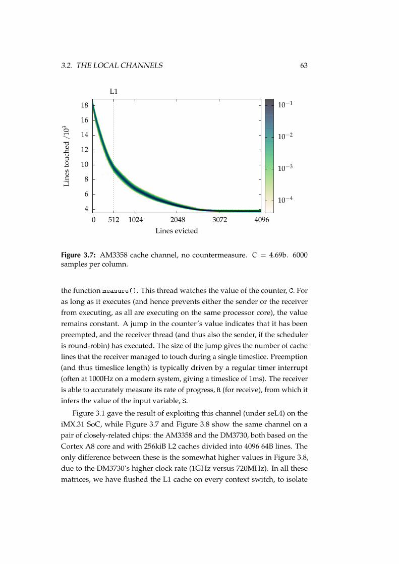
3.2. THE LOCAL CHANNELS 63Li
nes
touc
hed/
103
Lines evicted
4
6
8
10
12
14
16
18
5120 1024 2048 3072 4096
L1
10−4
10−3
10−2
10−1
Figure 3.7: AM3358 cache channel, no countermeasure. C = 4.69b. 6000samples per column.
the function measure(). This thread watches the value of the counter, C. Foras long as it executes (and hence prevents either the sender or the receiverfrom executing, as all are executing on the same processor core), the valueremains constant. A jump in the counter’s value indicates that it has beenpreempted, and the receiver thread (and thus also the sender, if the scheduleris round-robin) has executed. The size of the jump gives the number of cachelines that the receiver managed to touch during a single timeslice. Preemption(and thus timeslice length) is typically driven by a regular timer interrupt(often at 1000Hz on a modern system, giving a timeslice of 1ms). The receiveris able to accurately measure its rate of progress, R (for receive), from which itinfers the value of the input variable, S.
Figure 3.1 gave the result of exploiting this channel (under seL4) on theiMX.31 SoC, while Figure 3.7 and Figure 3.8 show the same channel on apair of closely-related chips: the AM3358 and the DM3730, both based on theCortex A8 core and with 256kiB L2 caches divided into 4096 64B lines. Theonly difference between these is the somewhat higher values in Figure 3.8,due to the DM3730’s higher clock rate (1GHz versus 720MHz). In all thesematrices, we have flushed the L1 cache on every context switch, to isolate

64 CHAPTER 3. CASE STUDY: PRACTICAL COUNTERMEASURES
Line
sto
uche
d/
103
Lines evicted
6
8
10
12
14
16
18
20
22
5120 1024 2048 3072 4096
L1
10−4
10−3
10−2
10−1
Figure 3.8: DM3730 cache channel, no countermeasure. C = 5.28b. 8000samples per column.
the effect of L2 contention. We will see that this flush is required for cachecolouring in any case, in Section 3.3.
The number of lines evicted by the sender, the input variable S—its work-ing set size, varies along the horizontal axis, while the number touched bythe receiver, the output variable R, along the vertical. The colour at point{s, r} gives the conditional probability of seeing r lines touched by the receiver,given that s were evicted by the sender. Intuitively, the more the figure variesfrom left to right, the more easily the receiver can distinguish two differentinput values, and the higher the channel capacity.
The calculated capacity of 4.69b for Figure 3.7, and of 5.28b for Figure 3.8translate into usable bandwidths of 1.56 and 1.76kB/s respectively, whenmultiplied by 333Hz (the rate at which the ensemble of three threads completeone cycle of preemptions). A higher bandwidth can obviously be achievedby using a higher sample rate: On a uniprocessor, the useful sampling rate islimited by the preemption rate (1000Hz) but on a multiprocessor (or in the caseof simultaneous multithreading), the sampling rate is essentially unlimitedas the sender and receiver need only execute a single memory access eachin order to communicate. In this case the channel might be exploited at a

3.2. THE LOCAL CHANNELS 65Li
nes
touc
hed/
103
Lines evicted
15
20
25
30
35
40
45
0 8192 16384 24576 32768
L1
10−4
10−3
10−2
10−1
Figure 3.9: Exynos4412 cache channel, no countermeasure. C = 7.04b. 1000samples per column.
very high bandwidth (megabytes per second, at least), but the capacity, or thenumber of bits transferred per sample will not increase. In fact, the capacity islikely to decrease somewhat, as the effect of noise will become greater as therange of variation that the sender exploits becomes smaller. We thus note thatthe quantity of importance is the capacity (in bits), and that the bandwidth (inbits per second) depends on the maximum sampling rate, which is generallyout of our control. However, reducing the capacity will reduce the bandwidth.From now on therefore, we quote only the channel capacity.
The next plot, Figure 3.9, is for the Samsung Exynos4412, a 4 core ARMCortex A9. This chip has a significantly larger L2 cache than any of theother ARM SoCs tested, at 1024kiB. It also returns to the 32B cache lines ofthe ARM11, giving 32,768 lines. As we see, this leads to the substantiallyincreased bandwidth of 7.04b, as the sender now has finer-grained controlover its degree of interference. A further increase in clock speed (to 1.4GHz),coupled with cache lines that are half as long, is again sufficient to explain theincrease in the peak rate from 22×103 to 45×103 lines touched per preemption.
Our final unmitigated channel matrix, Figure 3.10, is for the Intel Core2 Duo E6550. This is much larger and more powerful than any of the ARM

66 CHAPTER 3. CASE STUDY: PRACTICAL COUNTERMEASURES
Line
sto
uche
d/
103
Lines evicted
50
100
150
200
0 16384 32768 49152 65536
L1
10−4
10−3
10−2
10−1
Figure 3.10: E6550 cache channel, no countermeasure. C = 8.82b. 1000samples per column.
cores we have considered, and has a commensurately larger L2 cache, at4MiB. Cache lines are 64B. The peak work rate is significantly higher, at≈ 250×103, which the increase in clock speed alone (from 1.4GHz to 2.33GHz)is insufficient to explain. This core clearly has a significantly higher load/storecapability, and a greater L2 bandwidth to match. The result is a capacity of8.82b.
Figure 3.11 summarises the unmitigated channel results: The capacity ofthe L2 cache-contention channel scales roughly with the logarithm of the num-ber of L2 cache lines. The confounding factors in this plot are the varying clockspeeds (which, in fact, increase monotonically with cache size for the cores weconsider), and that the x86 kernel has a minimum preemption interval of 2ms,versus the 1ms of the ARM kernel, which would tend to slightly overstate thecapacity for the E6550. The dotted line is a linear model, fitted to the E6550.
The Bus Contention Channel
The second local channel that we analyse is one that only appears in systemswith multiple processors: bus contention. In a multiprocessor system, theprocessors will generally share not only some levels of the cache hierarchy

3.2. THE LOCAL CHANNELS 67
3
4
5
6
7
8
9
10
2048 4096 8192 16384 32768 65536 131072
Cha
nnel
capa
city/
b
L2 cache size / lines
log2(x) − α, fitted to E6550
iMX.31AM3358DM3730
Exynos4412
E6550
Figure 3.11: Channel capacity against L2 cache size in lines.
Line
sto
uche
d/
103
Lines evicted
300
350
400
450
500
550
600
0 512 1024 1536 2048
L1
10−3
10−2
10−1
Figure 3.12: E6550 bus channel, no countermeasure. C = 5.80 5.815.80b. 3000
samples per column.
68 CHAPTER 3. CASE STUDY: PRACTICAL COUNTERMEASURES
(usually at least the last level), but they must also compete for bandwidth onsystem buses, e.g. to the memory or to peripherals. Thus, even if two processesexecute on separate processors, share no memory or other explicitly allocatedresources, and do not compete for cache lines, they can still interfere witheach other by monopolising bus cycles, which are typically underprovisionedrelative to the combined peak requirements of all processors.
Figure 3.12 shows the effect of contention between two processors, againexecuting the code of Figure 3.6, but this time with the sender and receivereach executing on one of the two separate cores of the E6550. On this chip,the two cores have separate L1 caches, but share a unified L2. The point atwhich the two processors begin competing for access to the L2 cache (andmemory) is clear in the figure, occurring as soon as the sender spills outsideits L1 cache. Here the interference is not due to competition for space, as theboth sender and receiver are restricted to only 2048 (out of 65, 536) cache lines,and thus see essentially no capacity or conflict misses. The effect is rather dueto the fact that the two cores combined are able to issue more load and storerequests (per second) than the L2 cache is capable of performing, and thusan increase in the number issued by the sender reduces the number availablefor the receiver. The capacity of this channel is between 5.80 and 5.81b (ournumerical precision in this example was limited to three significant figures).
This channel is obviously only measurable on the two multiprocessorplatforms (the E6550 and the Exynos4412), of which only the E6550 had aworking multiprocessor port of seL4 when our experiment began.
3.3 Cache Colouring
The first countermeasure that we consider, cache colouring, eliminates the cachecontention channel by exploiting a widespread feature of modern caches, set-associativity, to partition the cache between multiple domains.
Figure 3.13 illustrates the technique. Imagine a machine with a 256Bphysical address space addressed by an 8b word. In this machine, the memoryis divided into 16 frames, each of 16B. This is a simplified example, but theprinciples are identical for systems with much larger address spaces.
As already described, the cache is divided into lines, here of 4 bytes each,which are always a size-aligned block of adjacent bytes. The line is the smallestaddressable unit in the cache—loads and stores are always of a multiple of

3.3. CACHE COLOURING 69
000000000
0000111100010000
0001111100100000
0010111100110000
00111111
0
address
set
way
line
{offset
page {colour
7
1 2 3
1234567
6543210
Figure 3.13: Cache colouring.
the line size. Our system has 16 cache lines, for a total of 64 bytes of cache.The bytes within a line are indexed by the lowest bits of the address words, inour case bits 1 and 0.
For each load or store, the cache is searched to see if it holds the requestedaddress, and signals a miss if not. There are several approaches, the simplestbeing direct mapping: the line number is taken directly from the next lowestbits after the line offset. In our example, 16 lines require 4 address bits, andwe thus use bits 5–2. While simple to implement, a direct-mapped cache has asubstantial disadvantage: all addresses that are equal modulo the cache sizealias, and loading any will evict any other that is resident. Direct-mappedcaches suffer from a high rate of conflict misses.
The opposite extreme is the fully associative cache. Here, the address iscompared in parallel against every line, and a given line may thus be storedanywhere, irrespective of its address. A fully associative cache never suffersconflict misses, as any set of lines (of up to the cache size) may be co-resident.The disadvantages of the fully associative cache are that it is expensive toimplement, power hungry and the parallel match becomes slower as the cachebecomes larger. This is important, as the match is in the critical path.
The usual compromise between these is the set-associative cache. Herecache lines are divided into a number of associative sets. The set number is

70 CHAPTER 3. CASE STUDY: PRACTICAL COUNTERMEASURES
calculated by direct mapping, while the lookup within each set is associative.This takes advantage of the speed of direct mapping, while still allowingsome degree of co-residency for aliased addresses. The size of the sets, orassociativity, is the number of cache ways. For example, the iMX.31 has a 4-wayassociative L1 data cache of 512 lines, and thus has 128 direct-mapped sets.In contrast, the L2 cache of the E6550 is 16-way associative, with 65,536 lines,giving 4096 sets. Higher associativity is usually seen in outer-level caches,where latency is less critical.
Returning to our example, our 2-way associative, 16-line cache has 8 sets.These are indexed by the next 3 bits after the line offset: 4–2. The 2-wayassociativity has reduced the number of direct-mapped bits from 4 to 3 (2n
way associativity eliminates n direct-mapped bits). Any contiguous set of23+2 = 32 addresses will map one 4-byte line into every cache set. Theimportant point is that this range, the direct-mapped range, is larger than thepage size of 16 bytes. Therefore, any adjacent pair of pages will map ontodisjoint ranges of cache lines, as shown in Figure 3.13. We thus divide thephysical address space into pools of coloured pages, such that no two pages fromdifferent pools can collide in the cache. If processes are assigned to distinctpools (using the virtual-memory system to map these non-adjacent frames intoa contiguous range of virtual pages), then the cache channel between them isremoved.
We can only colour memory when the size of the direct-mapped rangeis at least two pages, and the number of colours available (the size of therange divided by the smallest page size) varies greatly between platforms.For the L2 cache, there are 4 colours available on the iMX.31, and 8, 8, 16 and64 for the AM3358, DM3730, Exynos4412 and E6550, respectively. We cannotcolour the L1 cache, as on every platform it either has only a single colour, oris virtually-indexed. We instead flush it on every context switch. The cost ofthis is relatively small, given its small size.
Turning to our results, Figure 3.2 showed the result of applying two-waycache colouring on the iMX.31, and Figure 3.14 and Figure 3.15 give the equiv-alent result for the two Cortex A8 cores, the AM3358 and DM3730. In contrastwith the unmitigated channels in Figure 3.1, Figure 3.14 and Figure 3.15 re-spectively, all visible variation has been eliminated. The capacities drop by afactor of 200, 400 and 1000 respectively, to on the order of a hundredth of abit. Note that all three results fail the statistical test introduced in Figure 3.1,

3.3. CACHE COLOURING 71
3.3
3.4
3.5
3.6
3.7
3.8
3.9
0 1024 2048 3072 4096
Line
sto
uche
d/
103
Lines evicted
10−5
10−4
10−3
Figure 3.14: AM3358 cache channel, partitioned. C = 1.51× 10⁻²b. CImax0 =
8.10× 10⁻³b. 49,600 samples per column.
4.5
4.6
4.7
0 1024 2048 3072 4096
Line
sto
uche
d/
103
Lines evicted
10−5
10−4
10−3
10−2
Figure 3.15: DM3730 cache channel, partitioned. C = 5.02 5.025.01 × 10−3b.
CImax0 = 2.75× 10⁻³b. 63,200 samples per column.

72 CHAPTER 3. CASE STUDY: PRACTICAL COUNTERMEASURES
Line
sto
uche
d/
103
Lines evicted
4.6
4.7
5120 1024 2048 3072 4096
L1
Figure 3.16: DM3730 cache channel, partitioned, showing L1 contention.
implying that there is a real residual channel here. We will return to this pointshortly, and show that this residual channel is due to TLB contention.
Figure 3.16 shows the effect of not flushing the L1 cache on the DM3730.The number of samples is insufficient to reliably estimate capacity, but theexistence of a channel is obvious.
Figure 3.17 shows the results on the Exynos4412, reducing the capacity ofFigure 3.9 by a factor of less than 100, from 7.04b to 8.13 × 10⁻²b. Togetherwith the apparent capacity lying above the threshold of 4.37× 10⁻²b, it is clearthat the residual channel is now seriously undermining the countermeasure.
The cause of this remaining channel is clear from the top blue curve ofFigure 3.18, which plots the expected value of each column of Figure 3.17.The variation of about 5 parts in 10, 000 is obvious, and is consistent with thecorresponding blue curve in the lower plot, showing the number of CPU stallcycles due to TLB misses per line touched by the receiver. A larger number ofTLB misses leads to a smaller number of lines touched.
The TLB, or translation lookaside buffer, is a small per-processor cache ofvirtual-to-physical address translations, which must be consulted on everymemory access, to determine the correct physical address to issue to theexternal memory subsystem. This cache is shared between processes and is

3.3. CACHE COLOURING 73
12.1
12.2
12.3
12.4
12.5
0 8192 16384 24576 32768
Line
sto
uche
d/
103
Lines evicted
10−5
10−4
10−3
10−2
Figure 3.17: Exynos4412 cache channel, partitioned. C = 8.138.148.12 × 10−2b.
CImax0 = 4.37× 10⁻²b. 7200 samples per column.
a source of contention. Flushing the TLB when switching between domainseliminates the remaining contention, at the cost of a greater rate of TLB-induced stalls, as shown by the red curves. This channel also appears onall other ARM platforms tested, explaining all the residual capacities notedabove.
The residual TLB channel only became apparent after a large amount ofdata was collected, and we thus do not yet have sufficient data to verify theabsence of a channel (after flushing) to the level of precision represented byFigure 3.17. Figure 3.18 however, suggests that if any variation remains, it hasbeen reduced by at least an order of magnitude.
Finally, Figure 3.19 shows the effect of colouring the L2 cache of the E6550.In contrast to the ARM examples, here there is a distinct artefact at half thecache size, which is more clearly visible in the red curve which plots thecolumn averages, as in Figure 3.18. Here we see a clear effect at half thecache size, and another at the L1 size. The latter occurs as the x86 architectureprovides no mechanism to selectively flush the L1 cache, and so in this run itwas left alone on preemption, allowing the two threads to contend. Togetherwith the half-cache artefact, this leaves us with a bandwidth of 4.54× 10⁻¹b:

74 CHAPTER 3. CASE STUDY: PRACTICAL COUNTERMEASURES
0
10
20
30
40
50
Line
sto
uche
d−
1229
0
4
8
12
16
0 8192 16384 24576 32768
TLB
stal
ls/l
ine
Lines evicted
no flushflush
no flushflush
Figure 3.18: Exynos4412 TLB contention.
only a 20-fold reduction over the raw bandwidth of 8.82b.
The L1 interference can be reduced by manually overwriting the contentsof the cache on a context switch, by having the kernel walk an array of a smallmultiple of the L1 size. This is has non-trivial performance implications, andis only somewhat effective, as the bottom-most, blue, curve in Figure 3.19shows. It is unclear whether this residual channel can be closed on x86 withoutsubstantial performance cost, although colouring would be effective betweencores that share a colourable last-level cache, but with separate L1s.
The remaining artefact (at half the cache size) appears to be due to L2 cachemisses generated by the sender. To confirm this, the blue curve was generatedby reducing the sender’s coloured pool to cover only a quarter of the cache,rather than a half in all other examples. We see that the artefact moves neatlyto a quarter of the cache size—the point at which the sender starts to cause alarge number of capacity misses by evicting its own previously loaded lines.
This contention cannot directly affect the receiver, as the two are parti-
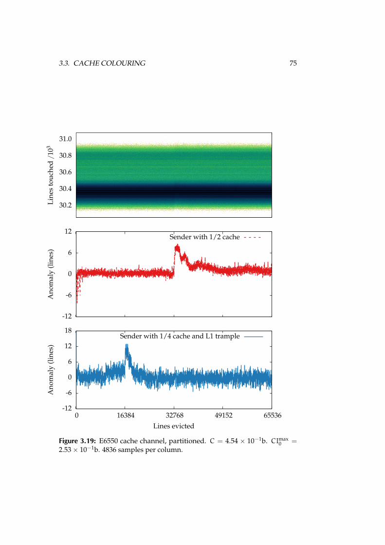
3.3. CACHE COLOURING 75
30.2
30.4
30.6
30.8
31.0
Line
sto
uche
d/
103
-12
-6
0
6
12
Ano
mal
y(l
ines
)
-12
-6
0
6
12
18
0 16384 32768 49152 65536
Ano
mal
y(l
ines
)
Lines evicted
Sender with 1/2 cache
Sender with 1/4 cache and L1 trample
Figure 3.19: E6550 cache channel, partitioned. C = 4.54 × 10⁻¹b. CImax0 =
2.53× 10⁻¹b. 4836 samples per column.

76 CHAPTER 3. CASE STUDY: PRACTICAL COUNTERMEASURES
27
28
29
30
0 1024 2048 3072 4096
Line
sto
uche
d/
103
Lines evicted
10−3
10−2
Figure 3.20: DM3730 cache channel, partitioned, with the receiver’s workingset restricted to 1024 lines. 2000 samples per column.
tioned, but certain cache misses in the kernel may still be observable. Bothkernel code and data are coloured, and hence partitioned, but there is a briefinterval between switching between coloured kernel images and resetting thepreemption timer, where a cache miss (particularly an instruction cache miss)can affect the length of the receiver’s timeslice. Specifically, the kernel resetsthe preemption timer, and hence starts counting time against the next thread’stimeslice before switching kernel images. The sender can cause cache missesin this interval (as we are still executing in its colour), that will be countedagainst the receiver’s timeslice. As the receiver uses its timeslice length tomeasure its progress, this will show up as an exploitable channel. This channelshould be resolved by a more careful re-implementation of kernel colouring,which is underway at the time of writing.
Performance Cost
Partitioning the cache is not without a cost. The effective cache size availableto any process is divided by the number of colours. If two processes werepreviously sharing the cache evenly, then this may have minimal impact onperformance, and could even show an improvement by better isolating them

3.3. CACHE COLOURING 77Li
nes
touc
hed/
103
Lines evicted
22
24
26
28
30
5120 1024 2048 3072 4096
L1
10−3
10−2
10−1
Figure 3.21: DM3730 cache channel, unmitigated, with the receiver’s workingset restricted to 1024 lines. 2000 samples per column.
[Tam et al., 2007]. In the case of a single process with a large working sethowever, we are likely to see a loss of throughput.
The receiver in our exploit represents the worst case: a process whoseworking set exactly matches the L2 size. Prior to partitioning, after a singlewalk through the array warms the cache, every subsequent access will bea hit. Halving the available cache by partitioning ensures that we will nowsee a miss on every access, as the process will evict all of its old cache linesbefore it gets a chance to reuse them. We see this in, for example, Figure 3.15,where the results cluster around 4600 iterations per timeslice, which mirrorsthe worst-case seen in Figure 3.8, where the receiver’s miss rate was drivento 100% by the sender. The worst-case penalty is thus a 5-fold reduction inperformance—consistent with simply having a smaller cache.
For a process whose working set fits within a partition, the situation ismuch better, as shown by Figure 3.20. Here, we have run the same receiverthread, but with its working set restricted to 1024 lines—comfortably withinits partition of 2048. Here we see no loss of throughput compared to theequivalent unpartitioned results in Figure 3.21, until the sender evicts 3/4 ofthe cache and begins to interfere with the receiver, causing the sudden drop at

78 CHAPTER 3. CASE STUDY: PRACTICAL COUNTERMEASURES
0
2
4
6
8
10
12
14
16
18
0 2 4 6 8 10 12
Inje
cted
nois
e(b
)
Capacity (b)
uncorrelatedanticorrelated
Figure 3.22: The effect of correlated versus anticorrelated noise on channelcapacity.
3072 lines.
Thus in performance terms, a partitioned cache behaves as a larger numberof smaller, separate caches.
3.4 Noise versus Determinism
We observed that to exploit a timing channel the receiver needs a clock. Forclocks (such as the preemption tick) that cannot be easily removed, there aretwo basic ways to prevent their use in exploiting a channel: reducing theirprecision by adding noise, or reducing the variation relative to observations inthe channel. Reducing variation can be viewed as adding anticorrelated noise,while the former approach uses uncorrelated noise.
Consider Figure 3.22. This plots the amount of noise required to reducethe capacity of a 12b channel to any desired level, assuming that it is eitheruniformly distributed and uncorrelated with the channel output, or perfectlyanticorrelated with it. To reduce the capacity to half its original value takesroughly the same quantity of noise in either case. Once we start trying toreduce the capacity toward zero, however, the uncorrelated noise required

3.5. INSTRUCTION-BASED SCHEDULING 79
increases rapidly. In fact, this curve has a vertical asymptote at zero—no quan-tity of noise will completely close the channel, some signal always remains.In contrast, given 12 bits of anticorrelated noise, the signal is gone and thechannel closed. Therefore, to reach small channel capacities, adding anticorre-lated noise—reducing the signal, is more effective. This insight underlies thesecond countermeasure we analyse.
3.5 Instruction-Based Scheduling
As already noted, it is not sufficient for the sender to influence the receiver’sperformance—the receiver must be able to detect it. This is the essence of thetwo-clock model for a timing channel [Wray, 1991]. This abstracts from the truepassage of time, requiring only the existence of two ‘clocks’, visible to thereceiver, which can be manipulated by the sender.
A clock, in this context, need only be a sequence of ticks, by observingwhich the receiver detects that some amount of time has passed. Given onlyone clock, the receiver has no idea how much time has elapsed since the lasttick, and if the ticks are not at a constant interval, this alone gives the receiverno information.
Once the receiver has a second clock, it can use its ticks to measure theintervals between those of the first—the receiver extracts information fromthe difference in the rate of the two clocks. If one clock does run at a constantrate (although the receiver, of course, does not know this), then the receivermeasures the true rate of the other. If the sender is able to manipulate one ofthe two clocks, without affecting the other, the rate measured by the receiverwill change. All that matters is that the sender can affect the relative rates ofthe two clocks, and that they are both visible to the receiver.
In general, the sender only needs to be able to affect the relative arrivalorder of two streams of events (the ticks), which are visible to the receiver.Conversely, if we can arrange that the relative arrival orders of all eventsvisible to the receiver are predictable (the clocks run at the same rate), thechannel disappears. This is the motivation for instruction-based scheduling,which attempts to prevent a process from using its own execution as a clock.
Returning to the cache channel, any process that shares a cache with thereceiver is a potential sender. The sender is able to manipulate the receiver’srate of progress by varying its cache usage. Thus, the receiver’s program counter

80 CHAPTER 3. CASE STUDY: PRACTICAL COUNTERMEASURES
C source ARM instructions x86 instructions1 mov %eax,%edx
2 shl $0x6,%edx
3 ldr r0, [r1,r3,lsl #5] mov 0x8059b80(%edx),%ecx
B[i][0]^= 1; 4 mvn r0, r0 not %ecx
5 str r0, [r1,r3,lsl #5] mov %ecx,0x8059b80(%edx)
6 ldr r0, [r2] mov 0x804f1c0,%edx
C++; 7 add r0, r0, #1 add $0x1,%edx
8 str r0, [r2] mov %edx,0x804f1c0
9 add r3, r3, #1 add $0x1,%eax
10 cmp r3, ip cmp $0x10000,%eax
11 movgt r3, #0 cmovge %ebx,%eax
while(1) 12 b 3 jmp 1
Figure 3.23: Disassembled machine code corresponding to lines 9–12 of thecache channel exploit in Figure 3.6.
forms a clock that the sender can manipulate. Note that the program counteris always implicitly available, even if the register itself is hidden—the receiverneed only run in a tight loop and count the number of iterations to measureits progress. The receiver now needs only one more clock, that isn’t tied to itsprogram counter, to exploit the channel. In Figure 3.6 we used the preemptiontick, assuming that all more straightforward clocks would be removed. Wethus attempt to tie the preemption tick to the receiver’s rate of progress, andthus make the channel unusable, without needing to remove the underlyingsource of interference.
Note that, in order to to be effective, all clocks need to be either removed, ormade deterministic with respect to each other. This is likely to be very difficultto achieve in a realistic system, especially if I/O is required. Instruction-basedscheduling has been implemented, specifically to address timing channels(e.g. by Stefan et al. [2013]), although its applicability to complete systemsis not yet established. What we establish here empirically, is the limitationsimposed on the technique by modern hardware.
Triggering preemptions based on the progress of a process is straightfor-ward. We take advantage of the performance counters that are available on anymodern CPU, and allow us to generate an interrupt once a fixed number ofinstructions have been retired. Replacing the timer interrupt in the seL4/ARMkernel with an interrupt generated by the PMU (Performance ManagementUnit) required the modification of only 18 lines of code. The implementationon seL4/x86 was not much harder.

3.5. INSTRUCTION-BASED SCHEDULING 81
-1
0
0 1024 2048 3072 4096
Line
sto
uche
d−
1000
0
Lines evicted
10−3
10−2
10−1
1
Figure 3.24: iMX.31 cache channel, instruction-based scheduling. C = 2.12×10⁻⁴b. CImax
0 = 5.41× 10⁻⁵b. 10,000 samples per column.
Figure 3.23 shows the machine code corresponding to the main receiverloop (lines 9–12 in function probe()) of Figure 3.6, for both ARM (the ARMv6and ARMv7 versions are identical at this point) and x86. Note that the nestedloops have been merged by the compiler. The loop on ARM is 10 instructionslong, while on x86 it takes 12. The two correspond almost one-to-one, with thetwo extra x86 instructions doing the work of the ARM barrel shifter, which canbe accessed by any arithmetic instruction. On ARM, the base of array B is heldin r1, and the address of the counter C in r2. On x86, these are at addresses0x8059b80 and 0x804f1c0, respectively. Setting the preemption interval to100000 instructions on ARM, and 120000 on x86, we expect to see 10000 loopiterations (and hence 10000 lines touched) per preemption.
Figure 3.24 shows the results for the iMX.31, with the baseline of 10000subtracted. The countermeasure behaves essentially perfectly here, with theoverwhelming majority of samples showing exactly 10000 iterations. Whilethe probability is so low that it is invisible, even on a log scale, we do veryrarely see 9999. This is due to the small number of instructions executed bythe kernel between resetting the preemption counter and returning to theuser-level thread. This means that slightly fewer than the desired 100000

82 CHAPTER 3. CASE STUDY: PRACTICAL COUNTERMEASURES
-1
0
1
0 1024 2048 3072 4096
Line
sto
uche
d−
1000
0
Lines evicted
10−4
10−3
10−2
10−1
1
Figure 3.25: AM3358 cache channel, instruction-based scheduling. C = 1.86×10⁻³b. CImax
0 = 9.56× 10⁻⁴b. 10,000 samples per column.
instructions are executed at user level, and thus the preemption point willslowly vary, resulting in the occasional short count of iterations. As this effectis not influenced by the sender, it does not constitute an exploitable channel.The true bandwidth is thus zero.
Figure 3.25 and Figure 3.26 show the results for the Cortex A8 cores: theAM3358 and the DM3730. Here, while the majority of samples give the ex-pected value, we see a nontrivial number at both +1 and −1, the frequencyof which is correlated with the sender’s eviction rate. This is a small, but ex-ploitable channel of capacity 1.86×10⁻³b for the AM3358, and 1.49×10⁻³b forthe DM3730. The deviations of +1 are correlated with those of −1, and look-ing at the raw sample data, we see why. Deviations from the nominal valuealways appear as a sequence of the form: . . . , 10000, 10001, 9999, 10000, . . . .That is, a single extra iteration in one preemption interval, and one fewer inthe next.
We would expect to see this behaviour if the preemption point wereslightly uncertain, but occurred just before the store that increments C atline 8 of Figure 3.23. Then, a slight delay in preemption would see one extrastore in the prior interval, and one fewer in the following. We infer that the

3.5. INSTRUCTION-BASED SCHEDULING 83
-1
0
1
0 1024 2048 3072 4096
Line
sto
uche
d−
1000
0
Lines evicted
10−4
10−3
10−2
10−1
1
Figure 3.26: DM3730 cache channel, instruction-based scheduling. C = 1.49×10⁻³b. CImax
0 = 7.74× 10⁻⁴b. 10,000 samples per column.
instruction count is accurate in the long run, by observing that the long-termaverage of the iteration count is precisely 10000. It thus appears that, while thecount reported by the PMU is accurate, the delivery of the overflow interruptis delayed if one of the core’s two execution pipes is stalled on a cache miss.
In Figure 3.27, which gives the results for the Exynos4412, the residualvariation gets worse. Here we see a dramatic variation in the counter value atpreemption—far more than can be accounted for by a small variation in thepreemption point.
Apart from a small number of deviations of −1, which are consistent withour understanding for the iMX.31 (the small number of kernel instructionscausing slightly short intervals), we see that the number of instructions ex-ecuted is usually significantly greater than we expect, and that this error isstrongly affected by cache misses—this channel has a capacity of 1.22b. Underheavy contention, or a close to 100% probability of a miss, the most likelyresult is an overshoot of 4 iterations, or 40 instructions.
There is a clear discontinuity at around the L1 size, which we infer to bethe effect of a single L2 miss—with a working set much smaller that the L1there is only a small probability of a miss (as the sender will only be dirtying

84 CHAPTER 3. CASE STUDY: PRACTICAL COUNTERMEASURES
Line
sto
uche
d−
1000
0
Lines evicted
0
2
4
6
8
10
12
14
16
0 8192 16384 24576 32768
L1 way
10−4
10−3
10−2
10−1
Figure 3.27: Exynos4412 cache channel, instruction-based scheduling. C =1.19b. CImax
0 = 3.76× 10⁻³b. 1000 samples per column.
its own L1 cache lines), while with one much larger, a miss is almost certain.The most likely value for a small working set (no miss) is 10012, against10007 with a miss, with the relative likelihoods equal at the L1 size. Thissuggests an L2 miss penalty of 5 iterations, or 50 cycles. That there is nofurther variation within the range of the L1 cache is expected, as it is flushedon every preemption.
The documentation for this core states that the particular counter that werely on gives only an approximation of the number of speculatively-executedinstructions, which is in turn an even coarser approximation of the numberactually retired [Cortex A9 TRM, §11.4.1, table 11-5]. What is most interestingis that the error we see is exactly the opposite of that we would expect fromspeculation—counting speculated instructions should overestimate the truevalue, as some of these will be discarded. In contrast, this is an underestimate.
This fact suggests that what we are seeing is not (at least primarily) aninaccuracy in the instruction count, but imprecision in the delivery of theoverflow interrupt, which is consistent with what we saw on the Cortex-A8.On this hypothesis, we are seeing an interaction between the performancecounter and the relatively complex pipeline. The core appears to defer the

3.5. INSTRUCTION-BASED SCHEDULING 85
ARM instructions1 mcr 15, 0, r5, cr9, cr12, {5}
PMU load 2 mrc 15, 0, r2, cr9, cr13, {2}
3 mov r3, r5
4 add r3, r3, #1
5 and r0, r3, #255
Cache line store 6 str r0, [sl, r0, lsl #5]
7 cmp r3, r8
8 blt 49 mcr 15, 0, r5, cr9, cr12, {5}
PMU load 10 mrc 15, 0, r1, cr9, cr13, {2}
Figure 3.28: Code to test PMU accuracy in the presence of L2 cache misses.
exception until there is a pipeline stall, which naturally tends to happen earlierwhen the cache miss rate is higher.
To test this hypothesis, we run the code in Figure 3.28 on the Exynos4412.This measures the change in the instruction count after a known sequenceof instructions—10000 iterations of the loop between lines 4 and 8. Thecoprocessor operations on lines 2 & 10 load the counter, and we dirty one cacheline per iteration on line 6. We should see 50002 instructions executed betweenthe two counter loads, or 50003 if one endpoint is included (assuming that thecounter increments consistently either before or after the load instruction).
In fact, we consistently see a count of 50006 instructions which tells ustwo things: The first is that the branch misprediction that occurs on looptermination does contribute to the instruction count, with the branch itselfand the first two loop instructions being speculated (the store to memory isnot speculated). The second, and more interesting, fact is that the count is notaffected by L2 misses, which implies that the effect we see in Figure 3.27 is thedelayed delivery of the overflow exception.
The result of instruction-based scheduling on the Cortex A9 is disappoint-ing, giving only a 5.8-fold improvement: from 7.04 to 1.22b, and this samecore gave the weakest performance under colouring. As an experiment, Fig-ure 3.29 shows the channel with both countermeasures enabled. Relative topartitioning alone, relaxed determinism gives a further 3.5-fold improvement:from 8.13×10⁻² to 2.32×10⁻²b, our best result on this platform. Whether thissmall additional improvement is worth the hassle of removing all remainingclocks is not clear.
Figure 3.30 shows our results for the E6550 which, like the Exynos4412,
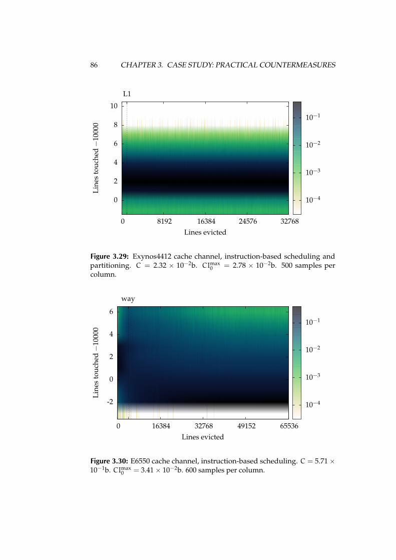
86 CHAPTER 3. CASE STUDY: PRACTICAL COUNTERMEASURES
Line
sto
uche
d−
1000
0
Lines evicted
0
2
4
6
8
10
0 8192 16384 24576 32768
L1
10−4
10−3
10−2
10−1
Figure 3.29: Exynos4412 cache channel, instruction-based scheduling andpartitioning. C = 2.32 × 10⁻²b. CImax
0 = 2.78 × 10⁻²b. 500 samples percolumn.
Line
sto
uche
d−
1000
0
Lines evicted
-2
0
2
4
6
0 16384 32768 49152 65536
way
10−4
10−3
10−2
10−1
Figure 3.30: E6550 cache channel, instruction-based scheduling. C = 5.71×10⁻¹b. CImax
0 = 3.41× 10⁻²b. 600 samples per column.

3.5. INSTRUCTION-BASED SCHEDULING 87Li
nes
touc
hed−
3883
30
Lines evicted
0
2
4
6
8
10
0 512 1024 1536 2048
L1
10−3
10−2
10−1
Figure 3.31: E6550 bus channel, relaxed determinism. C = 2.90 × 10⁻¹b.CImax
0 = 7.90× 10⁻³b. 3000 samples per column.
is a speculative, out-of-order CPU. Again, we see a variation in the numberof iterations per interval, but here clustered more tightly around the correctvalue, and not showing the consistent overshoot that we saw in Figure 3.27.This suggests that the integration of exceptions with speculation and out-of-order execution, on this core, is more precise. We still see a significantleft-to-right variation, correlated with the likelihood of a cache miss, givinga capacity of 5.71 × 10⁻¹b. The countermeasure is thus also comparativelyineffective on this core. We still appear to see exceptions being delayed untilpipeline stalls.
Instruction-Based Scheduling and the Bus Contention Channel
The great attraction of instruction-based scheduling is that it prevents (inprinciple), the exploitation of any timing channel, while an approach such ascache partitioning, while effective, is limited to a particular channel (in thiscase cache contention).
Figure 3.31 shows the result of applying IBS to the bus contention channelof Figure 3.12. While the magnitude of the effect is decreased by a factorof 200, 000, a clear artefact remains, and the capacity drops by only a factor

88 CHAPTER 3. CASE STUDY: PRACTICAL COUNTERMEASURES
of 15. This result is not surprising given that we already know that theperformance counter exception is affected by stall cycles, but it is neverthelessdisappointing. Nonetheless, this is the greatest reduction in bus-channelbandwidth that we were able to achieve.
Performance Cost
In contrast to colouring, which limits the cache available to a process, deter-minism has no intrinsic throughput cost. Where it is likely to hurt is in fairnessand latency.
Preemption is the means by which the CPU is shared between processes,and changing the conditions for preemption naturally affects fairness. Whilenormally each thread has an equal share, we instead enforce an equal sharingof work—each thread retires the same number of instructions per timeslice.The wrinkle is that these instructions may take a very different amount of timeto execute. At one extreme, a completely CPU-bound task that never stallswill complete in the minimum possible time. On the other hand a memory-bound task that stalls on almost every instruction will take dramaticallylonger. For example, a long sequence of pointer-chasing loads (where theaddress of the next load is calculated from the result of the previous, andthus cannot be speculated or prefetched) could well take 1000 times longer tocomplete than its CPU-bound competitor. Memory-bound tasks thus receivea proportionately higher share of CPU time than those that execute moreefficiently. Whether this is a problem depends on the application.
A further effect of the ballooning of timeslices is that latency, the maxi-mum interval between allocated timeslices, will increase. This may well be aproblem for a latency-sensitive application.
3.6 Lucky thirteen as a Remote Channel
Our final countermeasure deals with a different threat model: the remote at-tacker. This scenario presents us with a different set of tradeoffs than thoseconsidered so far. On the upside, remotely-exploited side channels are gener-ally of lower bandwidth, and the attacker has less ability to observe the system.On the downside, we have no control over the attacker itself. In particular, itmust be assumed to have an accurate clock, and hence an approach such asinstruction-based scheduling is impossible.

3.6. LUCKY THIRTEEN AS A REMOTE CHANNEL 89
The practicality of remotely exploiting a timing-based side channel againsta real system was demonstrated by Brumley and Boneh [2003]. Their workdemonstrates a real attack against OpenSSL, which exploited variation in theruntime of its implementation of RSA [Rivest et al., 1978] that depended bothon the secret key, and the attacker-supplied input. A notable feature of thisattack is that it could be carried out at a significant network distance from thetarget, opening up the possibility of attacks on internet-facing systems.
We likewise demonstrate that the lucky thirteen attack on OpenSSL’s im-plementation of datagram TLS (DTLS) reported by AlFardan and Paterson[2013] is exploitable at essentially unlimited network distance. We then showthat OS-level techniques can be used to effectively mitigate it, without requir-ing any modification of the vulnerable cryptographic implementation. Thisapproach is entirely black box.
The Attack
This attack exploits the fact that TLS first calculates the MAC (message au-thentication code, or digest), and then encrypts it. This allows a maliciousman-in-the-middle to modify packets taken from the wire and submit themto the server, which will then decrypt and begin to process them before theirauthenticity is established. In this case, the attacker exploits the non-constantexecution time of the MAC calculation itself by manipulating the paddingbytes contained in the packet. We construct two packets: M0 and M1, thattake a different length of time to process, before the server rejects them (asthe MAC check on the manipulated packet will fail), where this time dependson the (encrypted) contents. The attacker can thus distinguish two encryptedpackets by intercepting them and sending them to the server, on the client’sbehalf.
Figure 3.32 shows the distribution of response times for packetsM0 andM1, as measured at the greatest network distance we could achieve: betweenan Amazon EC2 datacenter in Oregon, USA and our lab in Sydney, Australia:a distance of 12,000km. While there is a substantial overlap between the dis-tributions, they are nevertheless easily distinguishable. An attacker observingonly a single round trip has a 62% chance of guessing which packet was sent.
Table 3.2 list the vulnerability for a number of different attack scenarios, allconducted against OpenSSL running on the AM3358. While the vulnerabilityclearly drops with increasing distance, it only does so rather slowly. We thus

90 CHAPTER 3. CASE STUDY: PRACTICAL COUNTERMEASURES
0
2
183 183.5 184 184.5 185 185.5 186
p/ms
Response time (ms)
M0M1
Figure 3.32: Histogram of DTLS echo times for OpenSSL 1.0.1c, at intercon-tinental distance—13 hops and 12, 000km, see row 4 of Table 3.2. Generatedfrom 105 samples per packet, and binned at 10µs. These peaks are distinguish-able with 62.4% probability.
Version Hops D(km) Vmax ML(b) RTT±σ(ms) Note
1.0.1c (VL) 1 0 0.998 0.986 0.734± 0.0073 0 0.597 0.109 1.193± 0.229 WLAN4 4 0.766 0.566 1.281± 0.05613 12,000 0.624 0.207 185.1± 31.47
1.0.1e (CT) 1 0 0.622 0.071 0.796± 0.0051.0.1c (SD) 1 0 0.570 0.030 0.751± 0.005
Table 3.2: Vulnerability against network distance.
conclude that network distance offers little or no protection against even quitesmall timing attacks (the underlying variation is less than 10µs).
Also included in this table is the vulnerability for the latest version ofOpenSSL (1.0.1e), which has replaced the vulnerable MAC calculation witha constant-time implementation. We see that the vulnerability is reduced,but not eliminated: an attacker can still guess with 62% probability. In thefollowing section we demonstrate that we can mitigate this channel more

3.7. SCHEDULED MESSAGE DELIVERY 91
effectively, and with lower overhead, using OS-level techniques. We quotemin leakage here, as we are concerned with vulnerability to a small numberof guesses.
3.7 Scheduled Message Delivery
Our countermeasure relies on the observation that an attack via the networkmust use channels that are under the control of the operating system. In seL4in particular, both synchronous communication (e.g. remote procedure callsor RPC) and asynchronous notification (e.g. interrupt delivery) are providedby kernel-managed objects: endpoints. We take advantage of this to imposea delay mechanism at the level of message delivery, to prevent the leakageof information via packet arrival times, without modifying the vulnerablecomponent itself.
Our threat model consists of a public-facing component that manipulatessensitive data. From its own perspective, the attacker has a direct channelto this sensitive component. In practice, this channel traverses at least onekernel-controlled endpoint, where we apply our countermeasure. This isimplemented as a lightweight mechanism, which implements the policy set bya separate user-level component.
We pace synchronous message delivery using real-time scheduling. Specif-ically, endpoints are modified to allow an authorised component to set aminimum response time, which is enforced by the kernel using a simplified EDF(earliest deadline first) scheduler.
Our prototype implementation is within seL4 itself, making high perfor-mance easier, although with careful design it could be replicated at user level,obviating the need for changes to the verified kernel.
The seL4 kernel already provides a mechanism for efficiently implement-ing RPC, the reply capability (cap). A client thread invokes the Call method (anseL4 system call) of an endpoint associated with the server. This transfers themessage payload synchronously, blocking the calling thread until the serverreplies. The server blocks on the same endpoint for client requests. Whenone arrives, the server receives both the message and a cap. This reply capfunctions as a one-shot endpoint: sending on it unblocks the client, deliveringthe reply and deleting the cap. This lets multiple clients use the same serviceendpoint, and the server direct its replies accordingly.

92 CHAPTER 3. CASE STUDY: PRACTICAL COUNTERMEASURES
We piggyback on this mechanism: the minimum response time of theendpoint sets the earliest instant at which the reply may be sent. When acall is made, the kernel records the instant of invocation, adds the delay, andstores this release time in the newly-created reply cap. If the server invokes thereply cap before the delay has elapsed, it blocks until it does. By default thedelay is set to zero, and the countermeasure is disabled.
Policy is provided by the user-level mitigator with the authority to set thedelay. This delay is set on the client side, allowing the mitigator to transpar-ently update it without the vulnerable server being aware. An existing servercan thus be used unmodified. The delay parameter provides a hook to allowthe mitigator to implement a dynamic delay policy. Zhang et al. [2011] presentjust such a policy, that adaptively adjusts the delay (with exponential backoff),such that under attack, the system will converge on its worst-case executiontime, while leaking a provably-bounded number of bits.
There is some potential for a malicious client to reduce the system’s per-formance by deliberately triggering the countermeasure. This is limited tothe worst-case response time which, as we will see in Figure 3.34 is only 10%greater than the unmitigated response time, even for an unrealistically toughexample. The extra time, moreover, is not wasted, but can be reclaimed foruseful work (or used to enter a low-power idle state).
The authority to set the delay is controlled by the standard capability sys-tem of seL4, which allows very flexible, fine-grained distribution of authority.A feedback channel is also provided to allow the mitigator to detect overrunsand adapt its policy.
As mentioned, delays are enforced by a simplified EDF scheduler: wemaintain a heap of pending events, sorted by increasing release time, andset the timer to expire at the first. We enforce no deadlines, which simplifiesimplementation. This is thus more accurately described as an earliest-release-first scheduler, and controls all time-triggered behaviour: preemptions arescheduled alongside message delivery.
Scheduled Delivery against Lucky Thirteen
Figure 3.33 shows how we use scheduled delivery to protect OpenSSL. Thesystem is partitioned into three layers, shown left-to-right, implemented byseparate components. The network stack (left) is lwIP [Dunkels, 2001], theTLS layer OpenSSL 1.0.1c, and the application an echo server. Data flow

3.7. SCHEDULED MESSAGE DELIVERY 93
in //
1
((
SSL_read // handler
oo
**3tt
4
R
~~out SSL_writeoo serveroo
2
C
>>
5jj
network TLS application
+∆t +3
Figure 3.33: Scheduled delivery for OpenSSL. Solid lines are packet flow withdotted control flow. Server blocks at C (call), until R (reply), after at least ∆t.
is shown by solid arrows and proceeds clockwise. Control flow is shownby the numbered dotted arrows, and begins with the server thread beingnotified of input (1). It then calls the handler to retrieve input (2), blocking (C)and creating a reply capability (R) with a delayed release time. The handlercalls OpenSSL (3) to retrieve decrypted packets. The attacker’s packets areprocessed by SSL_read, which may block, and returns once a valid packet isfound. The handler then restarts the server (4), which blocks until its delayexpires, and then forwards its output to SSL_write.
Figure 3.34 shows the response times for the two packets, as measuredfrom a directly-connected machine (no switch). In the terminology of Chap-ter 2, the packetsM0 andM1 are the two (secret) inputs to the channel, andthe response time is its output. Each pair of peaks for M0 and M1 (labelledVL, CT and SD respectively) in Figure 3.34 is essentially a channel matrix withjust two columns (M0 and M1), each built by taking 106 observations of theoutput for each input.
The leftmost pair of peaks (VL) are the response times for the vulnerableimplementation of OpenSSL 1.0.1c, executing on the AM3358. Times aremeasured, as in the original attack, by sending a modified packet immediatelyfollowed by a valid packet (also captured from the wire), and taking theresponse time of the second. This deals with the difficulty that DTLS doesnot acknowledge invalid packets. The machine under attack is executing anecho server, protected by DTLS. As line 1 of Table 3.2 shows, these peaks aretrivially distinguishable, allowing the attacker to correctly guess which packet

94 CHAPTER 3. CASE STUDY: PRACTICAL COUNTERMEASURES
0
0.2
725 750 775 800 825
p/µs
Response time (µs)
M0 VLM1 VLM0 CTM1 CTM0 SDM1 SD
Figure 3.34: DTLS distinguishing attack—histogram of response times forpacketM0 versusM1. Shows distinguishable peaks for vulnerable implemen-tation in OpenSSL 1.0.1c (VL), constant time implementation in 1.0.1e (CT),and results with scheduled delay (SD) demonstrating reduced latency. Allcurves generated from 106 packets for bothM0 andM1, and binned at 1µs.
was sent with 99.8% probability in the worst case. This corresponds to a leakof 0.986b of min entropy, out of 1 total.
The rightmost pair of peaks (CT) give the response time for the constant-time implementation of OpenSSL 1.0.1e, which substantially eliminates thevulnerability—the curves are almost identical. They are, however, not preciselyidentical, as row 5 of Table 3.2 shows—the two can still be distinguishedwith 62.2% probability, while to declare the system completely secure, theattacker should only be able to guess correctly half the time. This resultemphasises the difficulty of producing portable cross-platform constant-timecode, and indicates that the production version of OpenSSL (as of writing) isstill somewhat vulnerable to this attack.
Under scheduled delivery, any variation in the execution time of OpenSSL’sdecryption routines is absorbed between steps 2 and 4. The results obtained(after manually tuning the delay) are given by the central pair of peaks (la-belled SD) of Figure 3.34. As Table 3.2 shows, we (row 6) achieve a lower

3.7. SCHEDULED MESSAGE DELIVERY 95
vulnerability than the constant-time implementation (row 5) of OpenSSL1.0.1e (57% distinguishability or 0.03b leak of min entropy versus 62% and0.07b), with a 50µs (≈ 6%) better latency. The better matching between thecurves occurs as nothing in our implementation is data dependent, and theonly intrinsic latency penalty is the cost of blocking and restarting the serverthread, which we see from the figure is ≈ 10µs.
0
1
0 1000 2000 3000
CPU
load
Ingress rate (p/s)
1.0.1c1.0.1e
1.0.1c-sd 1 thread1.0.1c-sd 2 thread
Figure 3.35: Load performance and overhead of scheduled delivery againstunmodified OpenSSL 1.0.1c, and the constant-time implementation of 1.0.1e.
Figure 3.35 shows overhead at various loads. Each curve here plots CPUload against ingress rate, up to the point at which packet loss begins (thismachine has a single core). For the unmodified implementation (1.0.1c, blue),load increases linearly with packet rate, with packet loss beginning with theonset of saturation at 3000 packets per second (p/s). The constant-time imple-mentation of OpenSSL 1.0.1e (red) shows a 10.6% CPU overhead relative tothis baseline, consistent with the increased latency observed in Figure 3.34, andshows a correspondingly earlier saturation, at 2800 p/s. This extra CPU timeis wasted performing redundant computations, to ensure that the executiontime for any packet is always the worst case.
The next curve (green), for a single-threaded server using scheduled deliv-ery, tracks that for the original, vulnerable, implementation closely, showing

96 CHAPTER 3. CASE STUDY: PRACTICAL COUNTERMEASURES
only a 1.7% overhead. This shows the benefit of avoiding the redundantcomputations inherent in a constant-time implementation. Instead of busy-waiting (as in the improved SSL implementation), our implementation idlesby entering a (low-power) sleep state.
The same curve also demonstrates its weakness, with packet loss occurringat only 1400 p/s, as any packets that arrive while the server is sleeping aredropped, limiting achievable throughput. This benchmark is an extreme case,as the echo server does no work at all—all CPU time is devoted to OpenSSL.In a more realistic system, where the fraction of time devoted to vulnerablecryptographic routines is small, the throughput loss will be similarly low.
The orange curve is included to demonstrate that the slack time can bereclaimed. Here, we use two server threads to recover the sleep cycles (onecan respond while the other is delayed). This is not safe to do if the results arevisible to the attacker: running a second server thread (as we have done here)merely transforms exploitable latency variation into exploitable throughputvariation. In a more realistic setting, however, this is not necessary as, asdiscussed above, the amount of time wasted sleeping will in practice bedwarfed by the time spent executing the application.
3.8 Related Work
The publication of the orange-book standards for high-assurance systems[DoD] (now superseded by the common-criteria standards [NIST]) droveacademic and industrial interest in systems able to be certified to the highestlevels defined (e.g. A1), which required formal treatment of covert channels.
As already discussed, the VAX VMM project attempted to formally ad-dress timing channels, introducing the fuzzy time technique [Hu, 1991, 1992b;Trostle, 1993] to inject noise into all visible time sources. In contrast, we focusrather on reducing signal levels by mitigating channels directly, having notedthe limitations of adding uncorrelated noise to a channel. Numerous otherchannels were identified and analysed in connection with the project [Kargerand Wray, 1991; Wray, 1991], in particular bus contention (which we analyse)and the disk-arm channel (which we do not).
Our empirical approach has some similarity to more recent work of Gayet al. [2013], on measuring the bandwidth of interrupt-related covert channels.In contrast to our approach of calculating the bandwidth directly from a

3.8. RELATED WORK 97
sampled channel matrix, they hypothesise a binomial model for the leakagemechanism they analyse, and fit it to the observed data. The validity of themodel does not appear to have been extensively validated. We have theadvantage of not needing to provide such a model, although it could provideinsight into the underlying mechanism.
Cache colouring was originally proposed to allow real-time systems topartition the cache among tasks, in order to reduce contention-related jitter[Liedtke et al., 1997], and is still applied in contemporary systems [Ward et al.,2013]. Its potential as a mitigation technique was independently recognised byGodfrey [2013], who tested it on the Xen hypervisor against a live side-channelattack. Our results are complementary, showing by means of our syntheticbenchmark that the underlying channel is effectively mitigated. A furtherpoint of contrast is that we partition kernel as well as user memory.
StealthMem [Kim et al., 2012] cleverly exploits a widespread cache-replacementpolicy (k-LRU) to provide a limited quantity of memory that will never beevicted by a competing process. While effective, this approach suffers (alongwith colouring and instruction-based scheduling) from relying on undoc-umented (and non-guaranteed) hardware behaviour. In contrast to cachecolouring, it requires sensitive components to be modified to exploit theprotected memory, whereas we mitigate components as black boxes.
In contrast with fuzzy time, other authors have made the same realisationas us that increasing determinism is more effective than injecting noise, andhave repurposed deterministic execution frameworks, originally developedto aid in debugging multithreaded systems [Bergan et al., 2010; Aviram et al.,2010b,a; Ford, 2012], to mitigation. In contrast to this full determinism ap-proach, requiring modification of vulnerable components, instruction-basedscheduling, as implemented by us and in the Hails web application framework[Stefan et al., 2013], specifically targets timing channels and is thus simpler toimplement and importantly, black box.
The scheduled-delivery countermeasure is inspired by the work of Askarovet al. [2010] and Zhang et al. [2011] who showed how to adaptively set delaysin order to provide on-line defense against remote timing attacks. We presentan efficient, light-weight mechanism capable of implementing such a policy.
While in this work we analyse and mitigate known channels on modernhardware, incidentally discovering a few new ones, various authors have tack-led the difficult problem of systematically (or even automatically) identifying

98 CHAPTER 3. CASE STUDY: PRACTICAL COUNTERMEASURES
channels. The shared-resource-matrix methodology of Kemmerer [1983, 2002]provides a systematic approach to identifying potential channels throughknown mechanisms, and has been influential in the literature. The problemof channels through known (kernel) mechanisms does, however, appear tobe subsumed by more recent work on verified isolation [Murray et al., 2013].Sidebuster [Zhang et al., 2010], in contrast, is a more application-specific, andautomatic, approach to identifying a narrower class of channels: remotelyexploitable timing channels in web applications. No matter how channels areidentified, we argue that they require extensive empirical evaluation, withoutwhich any estimate of severity is, at best, an educated guess. In the caseof hardware-mediated channels, close analysis and a familiarity with thehardware remain essential.
There are other countermeasure approaches that we have not covered,for example the work of Gray [1993, 1994]. The focus of Gray’s work, andof much of the existing work in the field is on introducing noise, which weargue is an ineffective technique, when compared to increasing determinism,or eliminating contention. Lattice scheduling, an approach to minimising thenumber of cache flushes required to close the cache channel, due to Hu [1992a],is covered in more detail in Chapter 5, where we provide a formally-verifiedimplementation.
3.9 Conclusions
The results presented in this chapter allow us to reach a number of conclusionsregarding the effectiveness of mitigation, both by instantiating the models ofChapter 2 and observing the performance of the countermeasures on modernhardware.
Firstly, and unsurprisingly, the effect of unmitigated channels is devastat-ing. Every platform leaks at least 4 bits per observation via the cache channelwhich, even if limited to a relatively low sample rate (333Hz in our exam-ple) gives a bandwidth of kilobits per second. The bus contention channel issimilar. At these bandwidths, leaking a small but valuable secret, such as anencryption key, would require at most a few seconds. Even the transmission ofbulk data is feasible, especially on a multiprocessor where the sampling rate iseffectively unlimited. Even for the remote channel (the lucky thirteen attack),where the appropriate measure is no longer bandwidth but min leakage, we

3.9. CONCLUSIONS 99
see total compromise after only one observation: this system leaks 0.99 bitsof min-entropy (out of a total of 1 bit possible) in a single attempt, despitebeing a side and not a covert channel, and thus being accidentally, rather thandeliberately exploited. These figures are also well in excess of the 1b/s and0.1b/s permitted by the thirty year old orange-book standards [DoD]. Forsystems concerned with information leakage, effective countermeasures arethus essential.
We find that colouring is generally effective against the cache channel, aslong as care is taken to deal with all residual channels. We do see a trend ofdecreasing effectiveness on more complex hardware, with capacity reductionsof 200 to 1000 times for the simpler cores (the ARM1136 and Cortex A8),compared to less than 100 for the more complex A9 (Exynos4412) and Conroe(E6550) cores. In the case of the E6550, we are greatly restricted by the lack ofa mechanism to selectively flush the L1 cache, making it presently impossibleto achieve both high performance and high security on the x86 platform. Ourresults do not yet include the effect of TLB flushing, but we neverthelessconclude that cache colouring remains broadly effective, although harder toeffectively implement on recent hardware.
Instruction-based scheduling shows a similar pattern, but much more dra-matically. It drops from begin extremely effective on simpler cores (apparentlyperfect on the ARM1136, and thousand-fold reductions on the A8), to beingessentially useless on the A9 and Conroe cores. This is due to its reliance onthe accuracy of performance counters, which we have demonstrated to bepoor, and strongly affected by events under the sender’s control. The alterna-tive, of deliberately stopping short and then single-stepping the processor tothe required point, abandons the advantages of simplicity and inherently lowperformance impact that make the approach attractive. Combined with thenecessity of eliminating all timing sources available to the receiver leads us toconclude that this countermeasure is not practical. Even for the bus channel,its performance is poor enough not to be worth the effort.
It thus appears that while known countermeasures can be used to make asubstantial improvement in the capacity of local hardware-mediated channels,success is highly reliant on very careful implementation and empirical analysis,and depends on the effect of undocumented and evolving low-level hardwaredetails. For the time being, systems requiring a truly high level of localcovert-channel security will need to continue to use either fully isolated or

100 CHAPTER 3. CASE STUDY: PRACTICAL COUNTERMEASURES
specialised hardware. Cache colouring does, however, offer hope for reducingthe scope for side-channel attacks on sensitive cryptographic components,given a robust and practical implementation.
The outlook for remote channels is much more positive. We see thatwhile we do not yet have perfect mitigation for channels such as the luckythirteen attack, black-box techniques allow us to outperform the state-of-the-art solution (constant time reimplementation), with lower implementationeffort, better security and better performance. There is also nothing to suggestthat a more carefully audited and implemented mitigation could not achieveperfect security, at low performance cost. The contrast with the situation forlocal channels is stark, and highlights the extremely large security challengeposed by shared hardware.
Finally, these experiments provide us with the data to instantiate themathematical models we derived in Chapter 2, to see whether the level ofmitigation that we can achieve is sufficient to provide meaningful protectionagainst the established threat models. We take our very best (non-perfect)result, for instruction-based scheduling the DM3730, showing a residualchannel of no more than 1.49× 10⁻³b, and substitute the matrix of Figure 3.15for that of Figure 2.18.
This channel shows a min leakage of 4.32× 10⁻³b. Using the pessimisticmin leakage models of Section 2.7, and re-using the example secret distribu-tion, after 60 guesses we leak only 0.25b (out of 5.9b) of min entropy via theside channel, but already have a roughly 25% chance of guessing correctly sim-ply by knowing the prior distribution on secrets. So, in the case of a very weaksecret (6 characters selected nonuniformly from 6 possibilities), the effect ofside-channel leakage is dominated by intrinsic leakage. This implementationis safe (its vulnerability is mostly intrinsic), but only barely.
The situation reverses dramatically for a stronger secret: A strong (uni-formly random) 1024b secret could be completely transmitted in 700,000 sam-ples (about 35 minutes) by a trojan horse (exploiting this as a covert channel),and could be guessed with 50% probability in only 120,000 (about 6 minutes)by an attacker exploiting a worst-case side channel. Additionally, even thebest-case result for the remote channel, a min-leakage of 0.03b, implies a 50%chance compromise in only 15 guesses, although this can likely be improvedwith a more thorough implementation.
These results are all naturally pessimistic: they are the worst-case outcome

3.9. CONCLUSIONS 101
if the full possible bandwidth of the channel is exploited. Real attacks arelikely to be less effective, and systems somewhat more secure in practice.Nevertheless, our results indicate that the state of the art in implementingleakage-resistant systems on commodity hardware is a long way from al-lowing us to give comfortable security guarantees given the pessimism ofestablished leakage modelling theory, even if we are able to meet the ratherarbitrary guidelines specified for high-assurance software.


4 pGCL for Systems
This chapter draws on work first presented in the following paper:
David Cock. Verifying probabilistic correctness in Isabelle with pGCL. InProceedings of the 7th Systems Software Verification, pages 1–10, Sydney,
Australia, November 2012. Electronic Proceedings in Theoretical ComputerScience. doi:10.4204/EPTCS.102.15
After establishing our threat model, the guessing attack, and our approachto modelling leakage in Chapter 2, and evaluating the effectiveness of low-level mitigation strategies in Chapter 3, we now consider how the problemcan be attacked from the other end—formally verifying the absence of (orlimits on) leakage using a high-level specification. To do so, we need to bringprobabilistic properties within the scope of an seL4-style proof.
The seL4 theorem [Klein et al., 2009] is a refinement from an abstractspecification, via an intermediate executable model [Derrin et al., 2006], toa high-performance C implementation [Winwood et al., 2009]. The higherlevels are specified in a locally-developed monadic framework [Cock et al.,2008], which allowed us to model the highly imperative style of the kernelin the pure executable fragment of the Isabelle [Nipkow et al., 2002] theoremprover’s mechanised higher-order logic (Isabelle/HOL).
Additional variables (such as time) can be added to a such monadic speci-fication, by extending the state type appropriately and stating how the systemacts on it. What we cannot yet handle is the stochastic nature of these variables.The execution time of a complex system is seldom deterministic, and evenwhen it is theoretically predictable, doing so is often so complex that we are
103

104 CHAPTER 4. PGCL FOR SYSTEMS
forced to retreat to statistical models. Therefore, we extend our toolkit totackle statistical reasoning, without giving up existing capabilities.
To this end, we formalise the probabilistic guarded command language ofMcIver and Morgan [2004] (pGCL), in Isabelle/HOL. Using this, we can pro-duce machine-checked refinement proofs for probabilistic systems, buildingon the extensive prior work on pGCL. Our formalisation integrates cleanlywith our existing work, all of which is in Isabelle. We show that we can reuseexisting results about seL4, by mapping our existing monadic Hoare logic intopGCL.
We have not conducted a full-system proof of probabilistic non-functionalproperties on the scale of L4.verified, but in this and the next two chapters,we demonstrate that the required tools are largely in place.
4.1 The Case for Probabilistic Correctness
The verification of the seL4 microkernel demonstrated that we can verify thefunctional correctness of real systems. Functional correctness, however, coversonly properties that are guaranteed to hold. This excludes classes of proper-ties relevant in practice, for example execution time. By allowing securityproperties that hold only with some probability, we can give a more nuancedclassification of systems than with a functional property such as noninterfer-ence [Goguen and Meseguer, 1982]. In particular, we wish to classify systemsaccording to the Shannon capacity, or min capacity, of identified side channels.
Probabilistic Behaviour in Systems
In formal specification, it is convenient to treat a system as predictable, andmake absolute claims about its behaviour. Once implemented, while thesystem may be predictable in principle, its size and complexity (and oftenunder-specification) makes this impractical.
The usual approach in this case is to retreat to a probabilistic model,informed by benchmarking. That this is true is apparent on reading the evalu-ation section of a systems paper: While the precise performance of a systemis theoretically predictable and could thus be calculated, what we see arebenchmarks and histograms. The tools of the evaluator are experiments andstatistics! This is a testament to the immense difficulty of precisely predicting

4.1. THE CASE FOR PROBABILISTIC CORRECTNESS 105
performance. Once real world phenomena intrude, as in networking, exactprediction becomes impossible, even in theory.
Moreover, some properties can only be treated statistically. If such prop-erties are correctness-critical, any proof must involve probabilistic reasoning.Our particular concern is variable execution time, particularly where it givesrise to leakage channels. Recall Figure 2.17, showing the response time ofa system using strcmp. Reasoning about the distribution of response timeswas crucial in calculating the channel capacity. This is a correctness-criticalsecurity property that is unavoidably probabilistic.
Security Properties
Returning again to the guessing attack, imagine that our adversary guesses indecreasing order of probability, updating these probabilities dynamically, asdid the optimal attacker described in Section 2.4. Here, as there, our securitycondition is that it does not guess correctly in fewer than k attempts.
For a functional security property, we would calculate the set of initialstates that guarantee that the property holds in the final state: its weakestprecondition (wp). Security could be assured by showing that the initial statelies in this set.
In a probabilistic system, however, it might be that from any initial state,there is a nonzero (albeit small) probability that the final state is insecure. Thisoccurs, for example, if the attacker guesses randomly. The most we could thenhope to find is the probability that the final state is secure.
What we need is a probabilistic analogue of the weakest precondition.Consider the weakest precondition as a function that takes only the value 0or 1, depending on whether a state is in the weakest precondition set or not.Could we instead return some value between 0 and 1? Instead of answering“secure” or “not secure” for a state, answering “secure with probability p”?We could then show that the system remains secure with probability > p, ifwp > p in the initial state. In pGCL we find just such an analogue. This is anextension of Dijkstra’s guarded command language (GCL) [Dijkstra, 1975],with a unified treatment of both demonic and probabilistic nondeterminism.

106 CHAPTER 4. PGCL FOR SYSTEMS
Refinement and Security
The standard problem with refinement in security is nondeterminism. Writinga ; ; b for ‘do a then b’, c u d for ‘do c or d’, and h := x for ‘assign x to h’,consider the following program:
h := secret ; ; (l := 0 u l := 1) where secret ∈ {0, 1}
Let h (high) be hidden, and l (low) be visible. We wish to formalise thestatement: ‘The value in l doesn’t reveal the value in h’. Writing a v b for ‘brefines a’, meaning that every trace1 of b is also a trace of a, the following is avalid refinement:
h := secret ; ; l := h
This clearly violates the security property, but is permissible as every action ittakes, could have been taken by the specification.
For a propertyQ to survive refinement, writing ` for predicate entailment,we need that
a v b
wp a Q ` wp b Q whence by transitivity,
P ` wp a Q
P ` wp b Q
This simply states that any property that holds of the specification, holds ofthe implementation. We have demonstrated that some intuitively reasonableproperties are not preserved by refinement—we need to make sure we chooseone that is.
Returning to pGCL, we have a novel notion of entailment. We write2
P � Q for comparison defined pointwise i.e. ∀s. P s 6 Q s. If P � Q, thenP has a lower value in every state than does Q. We also write3 «P» for theembedding of the boolean predicate P as real-valued function (an expectation):
«P» s = if P s then 1 else 0 noting that P ` Q↔ «P» � «Q»
We can now model our guessing attack as:
(h := 0 u h := 1) ; ; (l := 0 1/2⊕ l := 1) (4.1)
1A trace is any sequence of valid states of a program. Trace refinement impliesthat the implementation is allowed to take any step that the specification can take.
2We differ in syntax, as the symbolV is not readily available within Isabelle3Again we differ, as the established syntax, [·], clashes with lists.

4.2. THE PGCL LANGUAGE 107
where the secret (h) is chosen nondeterministically, and the guess (l) ran-domly (a p⊕ b denotes probabilistic choice between programs a and b, withprobability p for a).
We inherit a family of structural refinement rules, for example a u b v a(a choice is refined by either alternative), and the following relations:
WP_REFINES
a v b
wp a Q � wp b Q whence
P � wp a Q
P � wp b Q
which are the probabilistic equivalents of the previous refinement conditions.We have therefore, that h := 0 ; ; (l := 0 1/2⊕ l := 1) is a refinement ofEquation 4.1, but importantly, (h := 0 u h := 1) ; ; l := h is not. In contrast todemonic choice, probabilistic choice cannot be refined away.
A refinement in pGCL establishes a predicate with at least as high a proba-bility as does its specification. Thus if our predicate is ‘the system is secure’,and we are content with establishing its minimum probability, refinement bydefinition only increases this.
This reasoning applies only to security predicates: security properties thatcan be established by inspecting only the current state. Not all properties canbe expressed in this way: some can only be expressed by considering someset of possible traces of the system. Our guessing-attack model, however,is carefully constructed such that security is only dependent on the currentstate: a system is secure (by definition), if the attacker has not yet guessedthe secret. While this property does refer to traces (specifically, the historyfrom any point), this can be modelled using a shadow variable: the list of pastactions is appended to the state. This is the approach we take in Chapter 6,where we formally derive leakage bounds on a guessing attack in pGCL.
The guessing attack model is thus refinement sound in pGCL.
4.2 The pGCL Language
We now summarise pGCL more completely, noting our small variations insyntax relative to the standard presentation. This summary is naturally in-complete, and the interested reader is directed to the aforementioned work ofMcIver and Morgan [2004].
Programs in pGCL have two interpretations: The first is as a probabilisticautomaton, moving from a starting state to some final state, with well-defined

108 CHAPTER 4. PGCL FOR SYSTEMS
probability. The second is as an expectation transformer, mapping a real-valuedfunction on final states (a post-expectation), to one on initial states (a pre-expectation). The weakest pre-expectation (wp, overloading this term) of apost-expectation at some initial state is the smallest expected value (minimisedover demonic choices) of the post-expectation in the final state. For example,the weakest pre-expectation of the expression x, under the program
(x := 1 1/2⊕ x := 0) u (x := 2 1/3⊕ x := 1)
is
min(
12× 1 +
12× 0) (
13× 2 +
23× 1)
=12
We mechanise the expectation-transformer interpretation, but the two areequivalent. The probabilistic automaton is generally more intuitive, givingthe most straightforward way to visualise results.
Programs are constructed using several operators, including some alreadymentioned:
• Sequential composition: a ; ; b.
Composition is interpreted either as ‘do a, then b’, in the automatoncase, or as ‘apply a to the result of b’ in the expectation transformer case.
• Name binding: n is f in a n, where f is a function from state to value.
This is purely syntactic, and simply binds a complex expression forreuse. This primitive is novel to our formalisation, but is a commonfeature of functional languages.
• Applying a state transformer: Apply f.
This is the primitive operator for state updates. It is usually hidden bythe syntax translations for records described below.
• Demonic choice: a u b ordx ∈ S. a x
The first of these is binary choice, which can be repeated in the obviousway to express any finite choice. The second is convenient for expressinga either a large finite choice or infinite branching. In doing so, wemust be careful that the program remains well-defined. For example,wp (
dx ∈ Z. Apply
(λ_. x
)x is not well-defined: there is no minimum
(or even a well-defined infimum) for x’s final value.

4.2. THE PGCL LANGUAGE 109
Rather than enforce this syntactically or through types, the user is forcedto discharge a verification condition that the primitive is well formed,for example by appealing to finiteness. Our reason for this is that wewill later (in Chapter 6) need to allow well-defined infinite choices, inorder to abstract over possible strategies for an attacker.
• Probabilistic choice: a p⊕ b, or 8 x ∈ S · a x@ P x
As for deterministic choice, but constrained by a particular distribution.The transformer interpretation is as the sum over possibilities, weightedby probability. This primitive is well defined even for infinite choices.
• Finite repetition: an = a ; ; . . . ; ; a︸ ︷︷ ︸n
.
• Lifting from a non-probabilistic monad: ExecM.
This connects with our existing work on monadic Hoare logic [Cock et al.,2008], by embedding a monad into pGCL. We return to this in Section 4.4,and again in Section 5.2, where we demonstrate its application and thelifting of Hoare triples.
• Recursion: µx. T x
Recursion is defined as the fixed point of a single recursive equation. Theµ operator binds a transformer (of type (σ → R) → σ → R), to whichthe recursive equation T is applied. We expand on this in Section 4.4.
• Looping: do G→ a od
This is syntactic sugar for recursion, see Equation 4.3.
• Failure: abort & Success: skip
The two remaining primitives are the diverging program abort, and thedo-nothing program skip.
While programs may have any state type, in practice we use Isabelle’srecord types: tuples with labelled fields, analogous to C structures. The advan-tage is that through syntax translations, we are able to use the field identifiers

110 CHAPTER 4. PGCL FOR SYSTEMS
as pGCL variable names. For example:
x := v =⇒ Apply(λs. x_update (λ_. v) s
)x :∈S =⇒
ls ∈ S. x := s
x :∈S atP x =⇒ 8 s ∈ S · x := s@ P s
The assertion language is shallowly embedded, closely resembling that ofGCL. There are a few novel probabilistic constructions:
• Entailment: P � Q ⇔ ∀s. P s 6 Q s usuallyV
• Conjunction: P&& Q ⇔ λs. max 0 (P s+Q s− 1) usually &
• Embedding: «P» ⇔ λs. if P s then 1 else 0 usually [P]
We have already introduced probabilistic entailment and embedding. Theform of probabilistic conjunction is chosen for compatibility with its booleanequivalent: «P» && «Q» = «λs. P s∧Q s». We use this particular form (ratherthan, for example P&& Q = λs. P s × Q s, which gives the same resultson embedded predicates) for technical reasons concerning the underlyingsemantic interpretation4.
The following is an example specification in expectation-entailment stylethat illustrates the essential features of the logic:
«P» && (λ_. p) � wp (a ; ; b) «Q»
This states that from any initial state satisfying P, after executing a followedby b, we reach a state satisfying Qwith probability at least p.
4.3 The pGCL Theory Package
We present a package of related theories, that implement a shallow embeddingof pGCL in Isabelle/HOL. The sources can be found in the pGCL subdirectory
4Briefly, the definition given is the only option that is sub-linear, a generalisation(to real-valued functions), and weakening, of the linearity condition required ofexpectation transformers in pure GCL. All sub-linear transformers are linear, andsub-linearity reduces to linearity in the case of embedded boolean predicates, but(for example) demonic choice, a u b = λs. min (a s) (b s), is not linear if a or b takevalues other than 0 and 1. All pGCL primitives are sub-linear. For further details, seeMcIver and Morgan [2004].
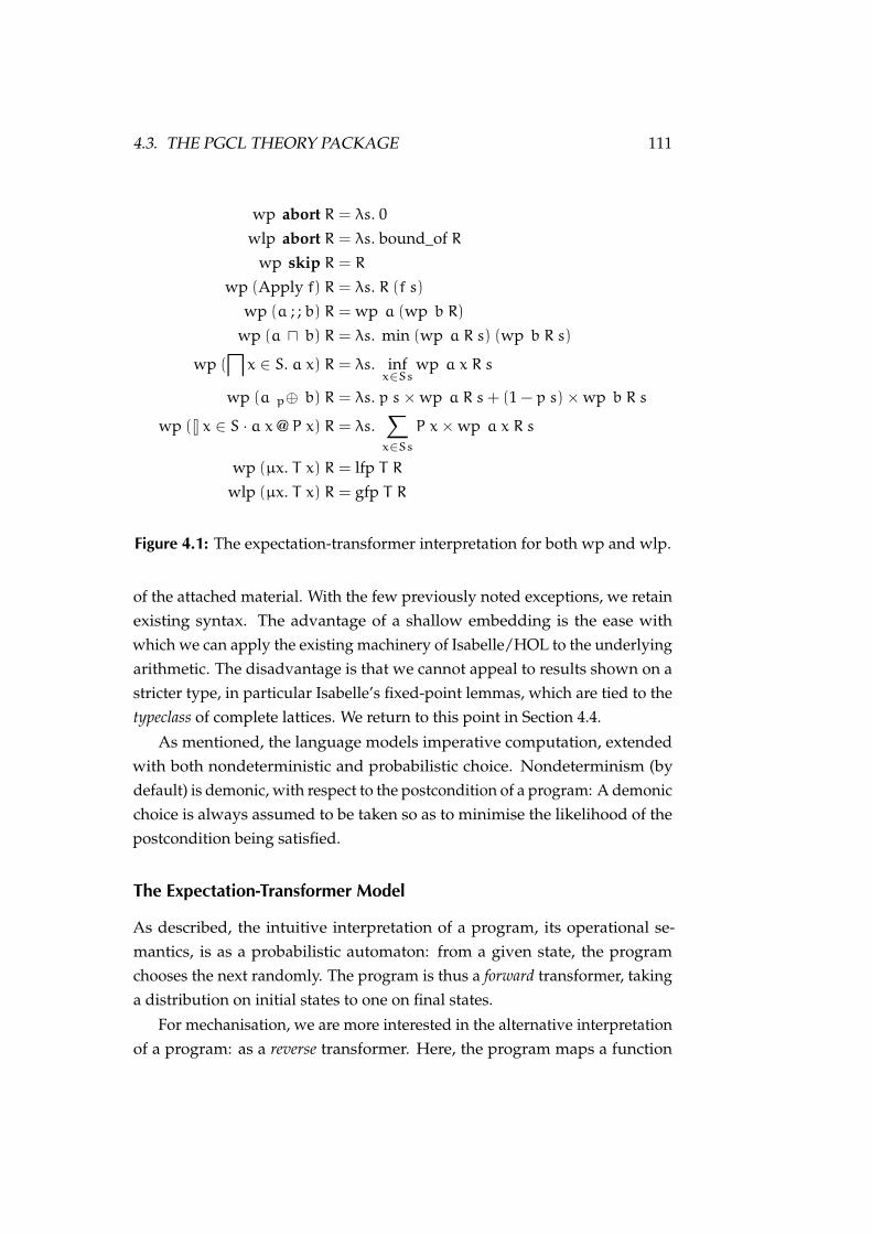
4.3. THE PGCL THEORY PACKAGE 111
wp abort R = λs. 0wlp abort R = λs. bound_of R
wp skip R = R
wp (Apply f) R = λs. R (f s)
wp (a ; ; b) R = wp a (wp b R)
wp (a u b) R = λs. min (wp a R s) (wp b R s)
wp (lx ∈ S. a x) R = λs. inf
x∈Sswp a x R s
wp (a p⊕ b) R = λs. p s×wp a R s+ (1 − p s)×wp b R s
wp (8 x ∈ S · a x@ P x) R = λs.∑x∈Ss
P x×wp a x R s
wp (µx. T x) R = lfp T Rwlp (µx. T x) R = gfp T R
Figure 4.1: The expectation-transformer interpretation for both wp and wlp.
of the attached material. With the few previously noted exceptions, we retainexisting syntax. The advantage of a shallow embedding is the ease withwhich we can apply the existing machinery of Isabelle/HOL to the underlyingarithmetic. The disadvantage is that we cannot appeal to results shown on astricter type, in particular Isabelle’s fixed-point lemmas, which are tied to thetypeclass of complete lattices. We return to this point in Section 4.4.
As mentioned, the language models imperative computation, extendedwith both nondeterministic and probabilistic choice. Nondeterminism (bydefault) is demonic, with respect to the postcondition of a program: A demonicchoice is always assumed to be taken so as to minimise the likelihood of thepostcondition being satisfied.
The Expectation-Transformer Model
As described, the intuitive interpretation of a program, its operational se-mantics, is as a probabilistic automaton: from a given state, the programchooses the next randomly. The program is thus a forward transformer, takinga distribution on initial states to one on final states.
For mechanisation, we are more interested in the alternative interpretationof a program: as a reverse transformer. Here, the program maps a function
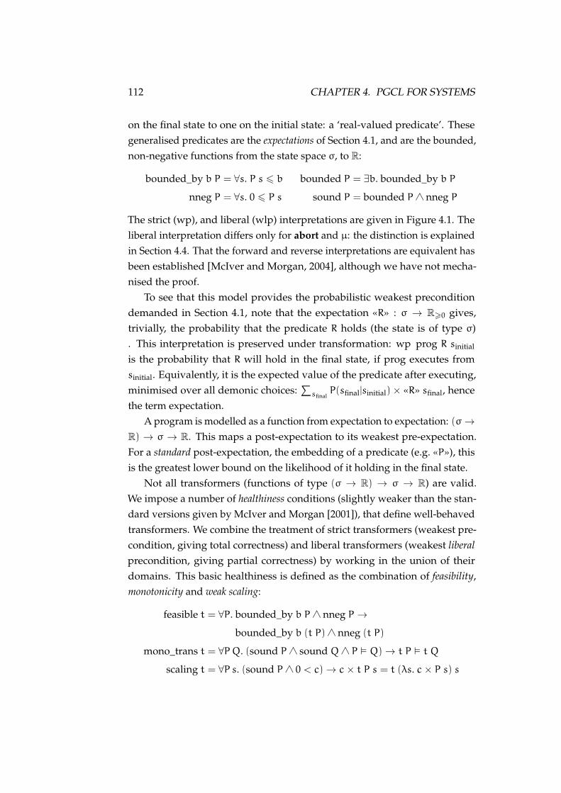
112 CHAPTER 4. PGCL FOR SYSTEMS
on the final state to one on the initial state: a ‘real-valued predicate’. Thesegeneralised predicates are the expectations of Section 4.1, and are the bounded,non-negative functions from the state space σ, to R:
bounded_by b P = ∀s. P s 6 b bounded P = ∃b. bounded_by b P
nneg P = ∀s. 0 6 P s sound P = bounded P ∧ nneg P
The strict (wp), and liberal (wlp) interpretations are given in Figure 4.1. Theliberal interpretation differs only for abort and µ: the distinction is explainedin Section 4.4. That the forward and reverse interpretations are equivalent hasbeen established [McIver and Morgan, 2004], although we have not mecha-nised the proof.
To see that this model provides the probabilistic weakest preconditiondemanded in Section 4.1, note that the expectation «R» : σ → R>0 gives,trivially, the probability that the predicate R holds (the state is of type σ). This interpretation is preserved under transformation: wp prog R sinitial
is the probability that R will hold in the final state, if prog executes fromsinitial. Equivalently, it is the expected value of the predicate after executing,minimised over all demonic choices:
∑sfinal
P(sfinal|sinitial)× «R» sfinal, hencethe term expectation.
A program is modelled as a function from expectation to expectation: (σ→R) → σ → R. This maps a post-expectation to its weakest pre-expectation.For a standard post-expectation, the embedding of a predicate (e.g. «P»), thisis the greatest lower bound on the likelihood of it holding in the final state.
Not all transformers (functions of type (σ → R) → σ → R) are valid.We impose a number of healthiness conditions (slightly weaker than the stan-dard versions given by McIver and Morgan [2001]), that define well-behavedtransformers. We combine the treatment of strict transformers (weakest pre-condition, giving total correctness) and liberal transformers (weakest liberalprecondition, giving partial correctness) by working in the union of theirdomains. This basic healthiness is defined as the combination of feasibility,monotonicity and weak scaling:
feasible t = ∀P. bounded_by b P ∧ nneg P →
bounded_by b (t P)∧ nneg (t P)
mono_trans t = ∀PQ. (sound P ∧ sound Q∧ P � Q)→ t P � t Q
scaling t = ∀P s. (sound P ∧ 0 < c)→ c× t P s = t (λs. c× P s) s

4.3. THE PGCL THEORY PACKAGE 113
hide = P := 1 u P := 2 u P := 3guess = G := 1 λs. 1/3⊕ (G := 2 λs. 1/2⊕ G := 3)
reveal = C :∈(λs. {1, 2, 3}− {P s, G s}
)switch = G :∈
(λs. {1, 2, 3}− {C s, G s}
)monty switch = hide ; ; guess ; ; reveal ; ; if switch then switch else skip
Figure 4.2: The Monty Hall game in pGCL.
Stronger results are established on-the-fly by appealing to one of severalsupplied rule sets.
A well-defined program has healthy strict and liberal interpretations,related appropriately:
well_def a = healthy (wp a)∧ healthy (wlp a)∧
(∀P. sound P → wp a � wlp a)
Reasoning with pGCL
The rules in Figure 4.1 evaluate the weakest pre-expectation of non-recursiveprogram fragments structurally. If the resulting term is not too large, thesimplifier can calculate it exactly. We also support two other approaches:Modular reasoning by structural decomposition, and the verification conditiongenerator (VCG). Examples are given in Isabelle proof script.
Consider Figure 4.2, a model of the Monty Hall problem [Selvin, 1975;Hurd et al., 2005]. The scenario is a game show: A prize is hidden behind oneof three doors (hide), of which the contestant then guesses one (guess). Thehost then opens a different door, (reveal), showing that it does not hide theprize. The contestant now chooses: to switch to the unopened door (switch),or to stick to the original (skip). Is the contestant is better off switching?
The victory condition, and hence the probability of the contestant winningand from a given starting state s, is given by the weakest precondition:
win g = (G g = P g) P(win) = wp (monty switch) «win» s

114 CHAPTER 4. PGCL FOR SYSTEMS
Proof by unfolding If switch is false, we can solve by explicitly unfolding therules in Figure 4.1. This approach was demonstrated by Hurd et al. [2005] Asexpected, the contestant has a 1/3 chance of success:
lemma wp_monty_switch: "λs. 1/3 � wp monty false �wins�"
unfolding monty_def hide_def guess_def reveal_def switch_def
by(simp add:wp_eval insert_Diff_if)
Proof by decomposition If switch is true the state space grows dramatically,and such a straightforward proof rapidly becomes infeasible (though it is stilljust possible in this case). Modular reasoning lets us scale further. Luckily, theweakest precondition semantics of pGCL admit familiar composition rules:
WP_STRENGTHEN_POST
P � wp p Q Q � R healthy (wpp) sound Q sound R
P � wp p R
WP_SEQ
Q � wp b R
P � wp a Q healthy (wp a) healthy (wp b) sound Q sound R
P � wp (a ; ; b) R
The healthiness and soundness obligations result from the shallow embed-ding.
To integrate with Isabelle’s calculational reasoner, we define probabilisticHoare5 triples:
WP_VALIDIP � wp a Q
{P} a {Q}
WP_VALIDD{P} a {Q}
P � wp a Q
VALID_SEQ
{P} a {Q}
{Q} b {R} healthy (wp a) healthy (wp b) sound Q sound R
{P} a ; ; b {R}
Note that VALID_SEQ is simply the composition of WP_COMPOSE with WP_VALIDIand WP_VALIDD.
5The classical Hoare triple {P} a {Q} states that if P holds initially then afterexecuting a, Q is guaranteed to hold.

4.3. THE PGCL THEORY PACKAGE 115
We need one final rule, peculiar to pGCL and its real-valued expectations:
WP_SCALE
P � wp a Q healthy (wp a) sound Q 0 < c
(λs. c× P s) � wp a (λs. c×Q s)
This follows from the healthiness of the transformer, and allows us to scalethe pre- and post-expectations such that the latter ‘fits under’ some target. Toillustrate, consider the ‘obvious’ specification of hide:
λs. 1 � wp hide «p ∈ {1, 2, 3}» (4.2)
This states that with probability 1, the prize ends up behind door 1, 2 or 3.In evaluating our preconditions stepwise, however, we find that the weakestprecondition of the remainder of the program is in fact:
λs. 2/3× «p ∈ {1, 2, 3}» s
Applying rule WP_SCALE to Equation 4.2 we derive a scaled rule:
λs. 2/3 � wp hide (λs. 2/3× «p ∈ {1, 2, 3}» s)
Finally the probability of success if the contestant switches is at least6 2/3:declare valid_Seq[trans]
lemma wp_monty_switch_modular: "λs. 2/3 � wp monty true �wins�"
proof(rule wp_validD)
note wp_validI[OF wp_scale, OF wp_hide, simplified]
also note wp_validI[OF wp_guess]
also note wp_validI[OF wp_reveal]
also note wp_validI[OF wp_switch]
finally show "λs. 2/3 � wp monty true �wins�"
unfolding monty_def
by(simp add:healthy_intros sound_intros monty_healthy)
qed
Here, we take advantage of the calculational reasoning facility of Isabelle,as described by Bauer and Wenzel [2001]. The intermediate Hoare triplesare automatically derived, by applying VALID_SEQ to the previous relationand the supplied specification. Finally, we again discharge all side conditionsusing the simplifier.
6In fact it is exactly 2/3, but our object is to demonstrate an entailment proof. Inmore complicated situations, calculating the exact pre-expectation is impractical.
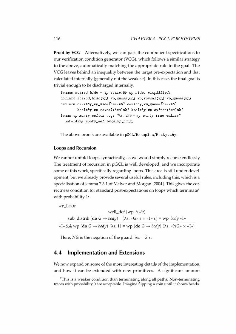
116 CHAPTER 4. PGCL FOR SYSTEMS
Proof by VCG Alternatively, we can pass the component specifications toour verification condition generator (VCG), which follows a similar strategyto the above, automatically matching the appropriate rule to the goal. TheVCG leaves behind an inequality between the target pre-expectation and thatcalculated internally (generally not the weakest). In this case, the final goal istrivial enough to be discharged internally.
lemmas scaled_hide = wp_scale[OF wp_hide, simplified]
declare scaled_hide[wp] wp_guess[wp] wp_reveal[wp] wp_guess[wp]
declare healthy_wp_hide[health] healthy_wp_guess[health]
healthy_wp_reveal[health] healthy_wp_switch[health]
lemma wp_monty_switch_vcg: "λs. 2/3 � wp monty true �wins�"
unfolding monty_def by(simp,pvcg)
The above proofs are available in pGCL/Examples/Monty.thy.
Loops and Recursion
We cannot unfold loops syntactically, as we would simply recurse endlessly.The treatment of recursion in pGCL is well developed, and we incorporatesome of this work, specifically regarding loops. This area is still under devel-opment, but we already provide several useful rules, including this, which is aspecialisation of lemma 7.3.1 of McIver and Morgan [2004]. This gives the cor-rectness condition for standard post-expectations on loops which terminate7
with probability 1:
WP_LOOP
well_def (wp body)sub_distrib (do G→ body) (λs. «G» s× «I» s) � wp body «I»
«I» && wp (do G→ body) (λs. 1) � wp (do G→ body) (λs. «NG»× «I»)
Here, NG is the negation of the guard: λs. ¬G s.
4.4 Implementation and Extensions
We now expand on some of the more interesting details of the implementation,and how it can be extended with new primitives. A significant amount
7This is a weaker condition than terminating along all paths: Non-terminatingtraces with probability 0 are acceptable. Imagine flipping a coin until it shows heads.

4.4. IMPLEMENTATION AND EXTENSIONS 117
a ; ; b = λab. (a ab) ◦ (b ab)abort = λab. if ab then λs. 0 else λs. bound_of P
Embed f = λab. fµx. prog x = λab. if ab then lfp_trans (λt. prog (Embed t) ab)
else gfp_trans (λt. prog (Embed t) ab)
wp a = a Truewlp a = a False
Figure 4.3: The underlying definitions of selected pGCL primitives.
of legwork was unfortunately necessary, as the existing infrastructure (thefixed-point theory) could not be straightforwardly applied to our semanticstructures, as we will shortly see.
Implementing wp and wlp
Figure 4.3 details the implementation of several primitives, together with thedefinitions of wp and wlp. Programs are represented as their associated trans-former, parameterised by the treatment of abort (the parameter ab), givingeither strict or liberal semantics. Only abort and µ change their behaviourbetween wp and wlp: The former gives either failure (λP s. 0) or success(λP s. bound_of P), whereas the latter is the least or the greatest fixed point,respectively. All others, as for (; ;), simply pass ab inward.
Consequences of a Shallow Embedding
The very shallow embedding used has two important consequences, the firstof which is negative. The healthiness of transformers, and soundness of expec-tations, must be explicitly carried as assumptions. A deeper embedding, suchas that of Hurd et al. [2005] could restrict to the type of healthy transformers,in which case these would be satisfied by the type axioms.
We avoid such an embedding to reuse as much of the mechanisation withinIsabelle/HOL as possible. Reasoning within a fresh type requires lifting (andmodifying) all necessary rules. The recent integration of the lifting packageinto Isabelle makes doing this simpler, but there is still a large body of existingautomation that would need to be reinvented. The burden of discharging

118 CHAPTER 4. PGCL FOR SYSTEMS
type_synonym (σ,α) nondet_monad =
σ⇒ (α× σ) set× bool{|P|} f {|Q|} = ∀s. P s→ (∀(r, s ′) ∈ fst (f s). Q r s ′)no_fail P m = ∀s. P s→ ¬(snd (m s))
Exec :: (σ,α) nondet_monad⇒ σ progExecM = λab R s.
let (SA, f) =M s in Run the monadif f then abort ab R s Fail is Abort
else if SA = {} then (bound_of R) Stuck is Successelse let S = snd „SA in Ignore result
glb (R „S) Infimum over states
Figure 4.4: The L4.verified non-deterministic monad in Isabelle.
our side conditions is, moreover, not high. For any primitively constructedprogram, healthiness follows by invoking the simplifier with the appropriatelemmas.
The positive consequence of an extremely shallow embedding is the easewith which it can be extended. We have already seen an example: the defini-tion of demonic choice from a set (following a standard abbreviation [McIverand Morgan, 2004]). To do so, one need only supply weakest-precondition(and weakest-liberal-precondition) rules, rules to infer healthiness and (op-tionally) rules for proof decomposition.
It is not necessary to show that the new primitive is sound, that is, producesa healthy transformer for all inputs. It is merely necessary that the suppliedrules show healthiness for just those cases in which it is actually used. Setdemonic choice is just such a partially sound primitive: Healthiness does notgenerally hold for infinite sets. Applied to finite sets, as it is here, the suppliedrules establish healthiness.
As a further example, we embed the non-deterministic monad at the heartof the L4.verified proof. The existing definition, Figure 4.4, is as a functionfrom states (σ) to a set of result (α), state pairs. The extra result is the failureflag, used to explicitly signal failure. This was added to ensure that termina-tion is preserved under refinement, as described elsewhere [Cock et al., 2008].

4.4. IMPLEMENTATION AND EXTENSIONS 119
We embed as follows: Stuck (no successor states) is success, for compatibilitywith our infimum-over-alternatives interpretation. Explicit failure is abort,which is in turn either success or failure under wp or wlp, respectively. Welift results as follows:
WP_EXEC
{P} prog {λr s. Q s} no_fail P prog ∃s. P s
«P» ` wp prog «Q»
WLP_EXEC
{P} prog {λr s. Q s} ∃s. P s
«P» ` wlp prog «Q»
Note that the difference between wp and wlp is simply termination.
Induction and the Lattices of Expectations and Transformers
Handling recursion means reasoning about fixed points. In this case, we needboth least and greatest, on expectations and transformers. Due to the shallowembedding, we cannot appeal to the existing fixed point results, which arephrased on a complete lattice. Neither the underlying type for expectations(α→ R) or for transformers ((α→ R)→ α→ R) can be so instantiated, dueto the lack of both top and bottom elements. The solution in each case isdifferent.
Sound expectations have an obvious bottom element, λs. 0, but there isno universal upper bound. We only require that there exists a bound for anygiven expectation. There need not exist any bound on an arbitrary set ofsound expectations. For example, with α = N, consider the set
{λs. if s = n then n else 0 : n ∈ N} .
Each expectation is bounded (by n) and non-negative, yet the least upperbound, λs. s is itself unbounded.
We need a surrogate for the top element. To illustrate, take our definitionfor greatest fixed point:
gfp_in f S = if ∃x ∈ S. x 6 f x then lub {x ∈ S. x 6 f x} else lowerbound S
A lower bound is easy (λs. 0), but in order to find the least upper bound,we need some upper bound. In a complete lattice, this is the top element.Instead, we appeal to feasibility:
bound_of ((µx. f x) Q) 6 bound_of Q

120 CHAPTER 4. PGCL FOR SYSTEMS
and thus
(µx. f x) Q 6 λs. bound_of Q .
It is therefore sufficient to consider fixed points that are weakly bounded by Q:
weakly_bounded_by Q = {R. sound R∧ bound_of R 6 bound_of Q}
Finally, we establish the standard fixed-point results parameterised by Q, forexample:
GFP_IN_UNFOLD
healthy t
gfp_in t (weakly_bounded_by P) = t (gfp_in t (weakly_bounded_by P))
The case of transformers is simpler, again due to feasibility:
t P s 6 bound_of P and thus t 6 λP s. bound_of P
Thus we have a top element, and establish a complete lattice by means of aquotient [Huffman, 2012].
le_trans t u = ∀P. sound P → t P 6 u P
equiv_trans t u = le_trans t u∧ le_trans u t
htrans_real t u = healthy t∧ healthy u∧ equiv_trans t u
quotient_type σ trans = (σ→ R)→ σ→ R /partial : htrans_rel
Using the induced homomorphism, we draw back the standard results:
GFP_TRANS_UNFOLD
∧t. healthy t ` healthy (T t)
∧t u. [healthy t; healthy u; le_trans t u] ` le_trans (T t) (T u)
equiv_trans (gfp_trans T) (T (gfp_trans T))
The Verification Condition Generator
The VCG (tactic pvcg), is simple but nonetheless capable handling Figure 4.2.It alternates applying an entailment rule, and attempting to discharge side-goals using internal and user-supplied rules.
The user supplies specifications as proved entailment rules, tagged with[wp], and healthiness rules, tagged with [health]. Internal rules are tagged[wp_core]. The VCG selects rules in this order:

4.5. RELATED WORK 121
1. User-supplied rules, as written.
2. User-supplied rules, with a strengthened postcondition:[wp_strengthen_post[OF rule]]. This leaves a side-goal that the post-condition of the supplied rule entails the strengthened version.
3. Internal rules.
A user-supplied rule will override an internal rule, and may refer directlyto a compound structure e.g. P � wp (a ; ; b) Q. The given rule will be usedrather than unfolding the composition. If no user rule is found, the VCG willproceed using its internal rules, calculating the exact weakest precondition byunfolding.
4.5 Related Work
The pGCL language of McIver and Morgan [2004] extends the treatment ofconventional nondeterministic programs, particularly that of Dijkstra [1975],from which the core syntax is derived. Treatments of the semantics of proba-bilistic programs had previously appeared, e.g. Kozen [1985], although thesetended to abandon classical nondeterministic choice in favour of probabilisticchoice. The work of McIver et. al. was the first to uniformly treat both formsof nondeterminism, in a standard verification framework.
Mathematically, calculating the weakest pre-expectation of program inpGCL is known to be equivalent [Gretz et al., 2014] to finding the expected re-ward for an appropriately-constructed Markov decision process (MDP) [Whiteand White, 1989]. There now exists a formal treatment of Markov models(including rewards) in Isabelle, due to Hölzl and Nipkow [2012]. We plan tounify this with our formalisation of pGCL, to provide it with an operationalsemantics, and a formal connection to Isabelle’s existing probability theory.
Interactive theorem provers, such as Isabelle, already host many existingmodels of programming language semantics [Nipkow, 2002; Mossakowskiet al., 2010; Cock et al., 2008; Harrison and Kieburtz, 2005]. Relative to these,the novelty here is that pGCL allows us to treat probabilistic properties andprograms.
A previous formalisation of pGCL, in the HOL4 theorem prover, waspresented by Hurd et al. [2005]. The principal difference to this work is the useof a deep, rather than shallow embedding. As we have described, our shallow

122 CHAPTER 4. PGCL FOR SYSTEMS
embedding allows us to take advantage of the powerful tool and theorysupport that Isabelle offers. The second advantage is the ease with which weare able to integrate other shallowly-embedded models, as demonstrated withthe nondeterministic monad. Our worked example, Monty Hall, is adaptedfrom theirs.
Coble [2010] investigated the problem of formally verifying anonymity in atheorem prover (HOL4). While the specific motivation is different (anonymityversus secrecy), the problems are quite close, and Coble also treats probabilityat length, providing a substantial library of formalised probability theory.Rather than taking such a ground-up approach, we have adopted an existinglogic (pGCL), and tackle probability in a comparatively simplistic manner,which has nevertheless proved adequate. Instead, we have invested moreeffort in developing a framework that should scale to larger, more realistic sys-tems, and in evaluating (and verifying) leakage measures other than Shannonentropy.
While we approach this area from the perspective of system security,others have arrived at similar approaches in the field of cryptography. Bartheet al. [2009] presented an automated theorem prover, CertiCrypt, tailoredto verifying provably-correct cryptographic algorithms. This tool has beensuperseded by the authors’ more recent EasyCrypt [Barthe et al., 2012b].
The language in which algorithms are expressed in these tools is quitesimilar to pGCL, incorporating true probabilistic choice alongside recursion.Although expressed in different terms, the language of Barthe et. al. incorpo-rates a notion of refinement: the monotone transformations. These are transfor-mations of a system model (here a game) that never decrease the probabilityof certain events. For game G and event A, a transformation h is monotone if(in the author’s syntax) PrG[A] 6 h(PrG′ [A′], or the probability of the trans-formed equivalent of event A, A′, in the transformed game G′, is at least ashigh as that of A in G. This is exactly the notion of refinement introduced inSection 4.1 for pGCL—refinement increases the probability of events.
The treatment of classical nondeterminism in CertiCrypt and EasyCryptis not as thorough as that of pGCL. Nondeterminism (expressed by distribu-tions that sum to less than one) is only introduced by non-termination or (forEasyCrypt) by assertions. In contrast, pGCL also provides nondeterministicchoice as a language primitive, which is essential in order to model classicalspecification–implementation refinement. It would probably be possible to

4.6. SUMMARY 123
unify the two languages, although the EasyCrypt semantics would need to bemodified. In particular, the transformers of Barthe et al. [2011] are assumed tobe additive i.e. µ(f+ g) = µf+ µg. Transformers in pGCL, however, are onlysub-additive: µf+µg 6 µ(f+g), and it is precisely nondeterministic choice thatintroduces strictly sub-additive transformers (recall that a nondeterministicchoice gives the least probability among the alternatives). The other assump-tions (monotonicity, multiplicative linearity, continuity) map precisely ontothe healthiness conditions of pGCL. Unifying the two approaches would bean interesting and potentially valuable project.
4.6 Summary
In this chapter, we stepped back from the low-level approach of Chapter 3, toconsider how we might reason formally about the sorts of stochastic behaviourthat we see in real covert and side channels. In particular, we need to find anapproach that fits with the refinement-driven correctness proof of seL4, whichforms the testbed for our more practical work.
Our approach is to take the existing language pGCL, and mechanise itslogic in the Isabelle/HOL theorem prover, as used in the L4.verified project.We have demonstrated a useful degree of automation, and the integration ofthe nondeterministic state monad that underlies the seL4 specification. Wereturn to this specific detail at more length in the following chapter, wherewe demonstrate that our mechanisation can be used to prove probabilisticsecurity properties for real systems.


5 Case Study —Lattice Scheduling
This chapter draws on work first presented in the following paper:
David Cock. Practical probability: Applying pGCL to lattice scheduling. InProceedings of the 4th International Conference on Interactive Theorem Proving,
pages 1–16, Rennes, France, July 2013. Springer.doi:10.1007/978-3-642-39634-2_23
As a more substantial example than that of Figure 4.3, we attack a muchlarger, and more obviously security-focused problem. Our goal is to demon-strate that mechanically verifying realistic probabilistic software, with proba-bilistic properties, is feasible. Our ‘realistic probabilistic program’ is a hybridprobabilistic lattice-lottery scheduler, designed to minimise the number offlushes required to completely close the cache channel (described in Sec-tion 3.2), while guaranteeing fairness and remaining simple and efficient.
The probabilistic properties of our program are: stochastic fairness — thatthe probability of starvation for any domain is zero, and non-leakage — thatthe distribution of observable outputs is independent of hidden inputs. Finally,we make our argument for feasibility by showing that we can incorporatethe existing seL4 results in a probabilistic setting. We are able to restrictprobabilistic reasoning to small regions, allowing the remainder of the proofto proceed in a traditional manner.
We begin with an abstract, nondeterministic specification, which we refineiteratively. Our first refinement is to a probabilistic version, and then to apractical implementation based on lottery scheduling. We demonstrate thatthis refinement could be continued using the L4.verified results. Finally, we
125

126 CHAPTER 5. CASE STUDY: LATTICE SCHEDULING
3 : {A,B}
1 : {A}
99
2 : {B}
ee
⊥ : { }
ee
OO
99
Figure 5.1: The classification/clearance lattice.
attach a hardware model, allowing us to demonstrate that we do in facteliminate leakage through the cache.
All lemmas in this chapter have been formally verified in Isabelle.
5.1 Security Policies and Covert Channels
Consider a hierarchically partitioned system, as depicted in Figure 5.1. Here,all data is classified with one (or both) of the labels A and B. An agent (pro-gram) may be cleared to process one, both, or neither of these, giving rise to 4clearance domains: 1 for A only, 2 for B only, 3 for both and ⊥ for neither. Ourgoal is to ensure that information derived from labelled data can only flowinto a domain cleared to process it. Enforcing such access policies, encom-passing explicit channels, is a well-studied problem [Denning, 1976]. We areinterested in eliminating flows through covert and side channels, specificallythe cache.
We again consider the cache contention channel introduced in Section 3.2.Recapping briefly, if two processes in distinct clearance domains (say 2 and 3)are executed on the same processor, they may be able to use cache contentionto communicate in violation of the security policy, even if all explicit channelsare removed. Exactly the same mechanism that we investigated previouslywould apply: the higher-clearance process (domain 3) can deliberately vary itsworking set, to evict some fraction of the lines belonging to the low-clearanceprocess (domain 2). As the low process can detect cache misses (as alreadydemonstrated), this forms a channel.

5.2. COUNTERMEASURES THROUGH REFINEMENT 127
3
��
1
??
2
__
��⊥
__ ??
Figure 5.2: The scheduling graph: S.
5.2 Countermeasures through Refinement
In this instance, we consider a different countermeasure to those alreadydescribed (colouring and instruction-based scheduling)—we flush the entirecache on a context switch. This will eliminate any interference, but it will notbe cheap: The Intel Xeon E7-8870, a high-end modern processor, has a 30MiBL3 cache, taking 2.5× 10⁶ cycles to refill (at the peak theoretical bandwidth ofthe memory subsystem), or 89% of the 2.8×10⁶ cycles per preemption intervalat 1000Hz. Nevertheless, the high degree of isolation offered by flushingmight make it worthwhile for a sufficiently sensitive system, especially if wecan amortise the cost.
A simple optimisation, due to Hu [1992a], is to exploit the security policyto avoid most cache flushes. In our partitioned system, it is acceptable to per-mit leakage from a domain to any higher domain—it is only necessary to flushwhen decreasing clearance level. This is the essence of lattice scheduling: Tran-sition upward in the classification lattice for as long as possible, before finallystarting again at the bottom, employing countermeasures (cache flushing) toprotect the downward transition.
To implement this, we construct the scheduling graph, S, Figure 5.2, from theclassification graph in Figure 5.1. The scheduling graph gives valid domaintransitions for the system, and contains only edges from the classificationgraph, or transitions to the downgrader1, ⊥. Downward transitions havedashed arrows. In the implementation, the cache is flushed on entering thedowngrader. We omit the edges from ⊥ to 3 and from 1 to ⊥ to emphasisethat not all edges need be included.
1The downgrader could just as easily be > in the lattice: it is trusted both to readfrom a high domain, and to write to a low domain, as it does nothing but flush thecache.

128 CHAPTER 5. CASE STUDY: LATTICE SCHEDULING
3
1.0
��
1
1.0??
2
0.5__
0.5
��⊥
0.25
__
0.75
??
Figure 5.3: The transition graph: T .
The conditions on the scheduling graph (modelled as a relation) are cap-tured as assumptions on S (encapsulated within an Isabelle locale), with themost important being downgrading:
Lemma 5 (Downgrading): If S allows a downward transition, it is to thedowngrader, ⊥:
(c,n) ∈ S clearance c * clearance n
n = ⊥
We specify the scheduler nondeterministically over the valid transitionsfrom the current domain, using the unconstrained demonic choice operator, :∈.
record stateA = current_domain :: dom_id
scheduleS =
c is current_domain in
current_domain :∈ (λ_. {n. (c,n) ∈ S})
The statement ‘x is y in (z x)’ binds the name x to the current value ofthe expression y, before evaluating z, while ‘y :∈ S’ updates the variable ynondeterministically, with some value from the set S.
A Randomised Scheduler
This classically nondeterministic specification, together with the downgradingproperty, captures the requirement that all downward transitions pass throughthe downgrader. As a practical specification however, it has a problem: itallows starvation. A refinement of this specification is free to follow any tracewithin the graph, for example (⊥, 2,⊥, 2, . . . ), never scheduling domain 3.
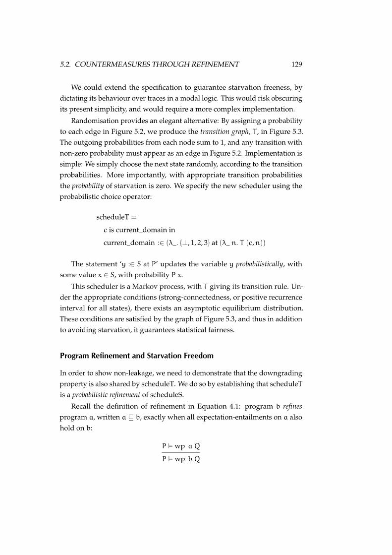
5.2. COUNTERMEASURES THROUGH REFINEMENT 129
We could extend the specification to guarantee starvation freeness, bydictating its behaviour over traces in a modal logic. This would risk obscuringits present simplicity, and would require a more complex implementation.
Randomisation provides an elegant alternative: By assigning a probabilityto each edge in Figure 5.2, we produce the transition graph, T , in Figure 5.3.The outgoing probabilities from each node sum to 1, and any transition withnon-zero probability must appear as an edge in Figure 5.2. Implementation issimple: We simply choose the next state randomly, according to the transitionprobabilities. More importantly, with appropriate transition probabilitiesthe probability of starvation is zero. We specify the new scheduler using theprobabilistic choice operator:
scheduleT =
c is current_domain in
current_domain :∈ (λ_. {⊥, 1, 2, 3} at (λ_ n. T (c,n))
The statement ‘y :∈ S at P’ updates the variable y probabilistically, withsome value x ∈ S, with probability P x.
This scheduler is a Markov process, with T giving its transition rule. Un-der the appropriate conditions (strong-connectedness, or positive recurrenceinterval for all states), there exists an asymptotic equilibrium distribution.These conditions are satisfied by the graph of Figure 5.3, and thus in additionto avoiding starvation, it guarantees statistical fairness.
Program Refinement and Starvation Freedom
In order to show non-leakage, we need to demonstrate that the downgradingproperty is also shared by scheduleT. We do so by establishing that scheduleTis a probabilistic refinement of scheduleS.
Recall the definition of refinement in Equation 4.1: program b refinesprogram a, written a v b, exactly when all expectation-entailments on a alsohold on b:
P � wp a Q
P � wp b Q

130 CHAPTER 5. CASE STUDY: LATTICE SCHEDULING
Lemma 6: The transition scheduler refines the lattice scheduler:
scheduleS v scheduleT
Proof. See theorem refines_ST in 'lattice_sched/LatticeSched.thy', inthe attached material.
Note that, in the terminology of pGCL, the specification of scheduleT iscompletely “deterministic”. Here we are referring to the absence of demonicnondeterminism. This terminology makes sense in light of the refinementorder: Demonic nondeterminism can be restricted by refinement, whereasprobabilistic choice cannot. Once a specification is fully probabilistic, it ismaximal in the refinement lattice, and one can take it no further. This impliesthat any further refinement is, in fact, semantic equivalence. We make use ofthis fact shortly, as a shortcut to establishing program correspondence.
Having fixed transition probabilities, we formally establish non-starvation.Proceeding in stages, we first show that starting in any domain, the probabilityof ending in domain ⊥ after 4 steps is at least 1/64:
(in_dom di)&&(λ_.
164
)� wp scheduleT4 (in_dom ⊥)
where
in_dom d = «λs. current_domain s = d»
We further establish that from domain ⊥, after a further 4 steps, there is anon-zero probability of ending in any desired final domain:
(in_dom ⊥)&&(λ_.
164
)� wp scheduleT4 (in_dom df)
Combining these, we have:(λ_.
14096
)� wp scheduleT8 (in_dom df) (5.1)
Finally:
Lemma 7 (Non-starvation): Taking at least 8 steps from any initial domain,we reach any final domain with non-zero probability:
∀s. 0 < wp scheduleT 8+n (in_dom df) s

5.2. COUNTERMEASURES THROUGH REFINEMENT 131
DOWNGRADING // scheduleS
��NON-STARVATION // scheduleT
Figure 5.4: First refinement diagram.
Proof. By induction on n. Equation 5.1 establishes the result for n = 0. Byinspection of Figure 5.3, we see that every domain is reachable in one step,and with non-zero probability, from at least one other, and thus if all domainsare reachable after n steps then all are reachable after n+ 1.
See also lemma nostarvation in 'lattice_sched/Fairness.thy'.
Note that this result is strictly stronger than the standard form of nonstar-vation, “Domain df is eventually scheduled.”: We have established that notonly is df eventually scheduled, it must always be scheduled within 8 steps,with some nonzero probability.
Figure 5.4 summarises these results. We have downgrading for sched-uleS and non-starvation for the probabilistic scheduleT, as indicated by thedotted arrows. Refinement is depicted as a solid arrow. The arrow direc-tions summarise the compositionality of results: composing with refinement,downgrading also holds for scheduleT, but non-starvation does not hold forscheduleS.
Data Refinement and the Lottery Scheduler
It is not sufficient to have an elegant specification, unless that specification canbe practically implemented. Therefore we implement our randomised latticescheduler as a lottery scheduler [Waldspurger and Weihl, 1994]. We then onlyneed the assumption of randomness for a single operation: drawing a ticket.
We extend the abstract state with a lottery for each domain. Every possiblesuccessor domain holds a certain set of tickets, given by the function ‘lottery’.To transition, the scheduler draws a ticket (a 32 bit word) and consults thetable to choose a successor. To emphasise that the probabilistic component canbe isolated, and to demonstrate compatibility with our existing framework,we divide the implementation into a core, in the nondeterministic state monad[Cock et al., 2008], which is then lifted into pGCL using the Exec operator,

132 CHAPTER 5. CASE STUDY: LATTICE SCHEDULING
allowing us to employ probabilistic choice. Both scheduleC and scheduleMoperate on the same state space: stateC. The syntax rLx := yM is an Isabellerecord update, assigning value y to field x of record r.
record domain = lottery :: 32 word⇒ dom_id
record stateC = current_domain :: dom_id
domains :: dom_id⇒ domain
scheduleM t = do c← gets current_domain
dl← gets domains
let n = lottery (dl c) t in
modify (λs. sLcurrent_domain := nM)
od
scheduleC = t from (λs. UNIV) at 2−32 in
Exec (scheduleM t)
The statement ‘x from S at P in (z x)’ binds the name x probabilisticallyfrom the set S (at probability P x), before evaluating z.
Having moved to a new state space, we cannot have direct programrefinement between scheduleT and scheduleC. Noting, however, that theabstract state can be recovered from the concrete by projection, we insteadhave (projective) probabilistic data refinement:
Definition 4 (Probabilistic Data Refinement): Program b, on state type σ,refines program a, state τ, given precondition G : σ → Bool and under pro-jection θ : σ→ τ, written a vG,θ b, exactly when any expectation entailmenton a implies the same for b, on the projected state and with a guarded pre-expectation:
P � wp a Q
«G» && (P ◦ θ) � wp b (Q ◦ θ)
Lemma 8: Let ‖S‖ be the cardinal measure (element count) of set S.
Under condition LR, that the lottery reflects the transition matrix,
T (c,n) = 2−32‖{t. lottery (domains s c) t = n}‖

5.2. COUNTERMEASURES THROUGH REFINEMENT 133
DOWNGRADING // scheduleS
��NON-STARVATION // scheduleT
φ,LR��
scheduleC
Figure 5.5: Second refinement diagram.
then under projection φ, which preserves the current domain,
current_domain (φ s) = current_domain s
scheduleC is a data refinement of scheduleT:
scheduleT vLR,φ scheduleC
Probabilistic Correspondence
As already mentioned, scheduleT is maximal in the refinement order, andthus any refinement is an equivalence. This is probabilistic correspondence:
Definition 5 (Probabilistic Correspondence): Programs a and b are saidto be in probabilistic correspondence, pcorres θ G a b, given condition G andunder projection θ if, for any post-expectationQ, the guarded pre-expectationscoincide:
«G» && (wp a Q ◦ θ) = «G» && wp b (Q ◦ θ)
Probabilistic correspondence is guarded equality on distributions: Froman initial state satisfying G, a and b establish Q with equal probability. Theadvantage of detouring via refinement, rather than directly showing corre-spondence, is that the proof is simpler: the next result follows directly fromLemma 8:
Lemma 9: The specifications scheduleT and scheduleC correspond givencondition LR and under projection φ:
pcorres φ LR scheduleT scheduleC

134 CHAPTER 5. CASE STUDY: LATTICE SCHEDULING
DOWNGRADING // scheduleS
��NON-STARVATION // scheduleT
φ,LR��
callKernelD
��
stepKernel ; ; scheduleC scheduleCφ,LR
ks
callKernelH
��callKernelC
Figure 5.6: Composed refinement diagram.
This extends Figure 5.4 to Figure 5.5, with correspondence indicated bythe double arrow. As correspondence implies refinement, both downgradingand non-starvation hold for scheduleC, as implied by the arrows. Propertiesrepresented by a single dotted arrow (e.g. downgrading), are preserved byboth refinement (single arrow) and correspondence (double arrow).
Proof Reuse: Composing with seL4
Our argument for the feasibility of this approach rests on the compatibilityof probabilistic correspondence with the non-probabilistic equivalent at theheart of the L4.verified proof. In Chapter 4, we demonstrated that monadicspecifications, in the style of seL4, can be re-used in a probabilistic setting, au-tomatically lifting Hoare triples to probabilistic predicate entailment relations.With the following result we go further, and lift the bulk of the refinementstack. The predicate corres_underlying in the following lemma is the funda-mental definition which underlies the refinement results at all levels of theL4.verified proof. Here, we need only note that this is the form of the top-leveltheorem2.
2Briefly, corres_underlying srel nf rrel G G′ mm′ is defined as:
∀(s, s′) ∈ srel. G s∧G′ s′ → (∀(r′, t′) ∈ fst (m′ s′).∃(r, t) ∈ fst (m s). (t, t′) ∈ srel ∧ rrel r r′ ∧ (nf→ ¬snd (m′ s′)))
5.2. COUNTERMEASURES THROUGH REFINEMENT 135
Lemma 10 (Lifting Correspondence): Given correspondence between monadicprogramsM andM′, with precondition G and projective state relation φ,
corres_underlying {(s, s ′). s = φ s′} True rrel G (G ◦ φ)MM′
whereM does not fail given G,
no_fail GM
and neither diverges without failing,
empty_failM empty_failM′
and thatM is deterministic on the image of the projection,
∀s. ∃(r, s′).M (φ s) = {(False, (r, s′))}
then we have probabilistic correspondence between their lifted counterparts:
pcorres φ (G ◦ φ) (ExecM) (ExecM′)
Note that the final assumption is exactly the determinism3 condition thatwe previously established for scheduleT, restricted to the components ofinterest. M is free to behave nondeterministically on components which aremasked by the projection.
We can thus compose our probabilistic results with the deterministic levelsof the L4.verified proof (the executable, or more recent deterministic abstractspecification [Matichuk and Murray, 2012]). For the problem at hand, it isonly necessary to make a few assumptions on the kernel:
Where guardsG andG′ hold on initial states s and s′ satisfying state relation srel, forany pair of (result, final state) obtained by executingm′, there exists a correspondingpair obtainable by executing m. If the non-failure flag, nf is set, then the predicateadditionally asserts thatm′ does not fail.
We use the predicate with a projective relation derived from φ, no failure, anarbitrary result relation, and a concrete guard which is the anti-projection of theabstract guard (G ◦ φ).
3 Determinism gives us correspondence, rather than just refinement. Considermonads A and A′, and variable x ∈ N, preserved by projection φA. Let A s benondeterministic, giving either sLx := x s + 1M or sLx := x s + 2M, while A′ s isdeterministic, giving sLx := x s+ 2M. All behaviours of A′ are included in A, and thuscorres_underlying holds. However, wp A x = λs. x s+ 1 whereas wp A′ (x ◦ φA) =λs. x s+ 2: a refinement, but not correspondence. As previously mentioned, if Aweredeterministic then by maximality, this refinement would be correspondence.

136 CHAPTER 5. CASE STUDY: LATTICE SCHEDULING
Lemma 11: If the kernel preserves the lottery relation,
{|LR|} stepKernel {|λ_. LR|}
and the current domain,
{|λs. CD s = d|} stepKernel {|λ_ s. CD s = d|}
and is total,
no_fail > stepKernel empty_fail stepKernel
then with the concrete scheduler, it refines the transition scheduler:
scheduleT vLR,φ stepKernel ; ; scheduleC
With this (again using refinement to show correspondence), Figure 5.5 be-comes Figure 5.6, now including the lifted kernel. The L4.verified refinementstack is depicted on the left to indicate how the results would compose, totake our result down to the real, executable kernel. Here callKernelD is thedeterministic refinement of original abstract specification of seL4, callKernelHis the executable model derived from the Haskell prototype, and callKer-nelC is the concrete model, comprising the final C and assembly languageimplementation
So far, we have only shown that our results are compatible: we do not yethave a mechanised proof. The remaining results are the first two assumptionsof Lemma 11, which will hold by construction as the existing kernel clearlycannot modify the additional scheduler state, and the fact that the state relationis projective: that is, that the abstract state is uniquely recoverable from theconcrete state. This is the intended behaviour of the state relation, and wehave no reason to suspect that this will not hold.
Non-leakage with a Concrete Machine Model
Our ultimate goal is to show the absence of information leakage via sharedstate (specifically the processor cache), and so we extend our scheduler with asimple hardware model. We model a private state per domain (memory), anda single shared state (cache):
record (sh,pr) machine = private :: dom_id⇒ pr
shared :: sh

5.2. COUNTERMEASURES THROUGH REFINEMENT 137
2
3
2
1
S
3
3
2
1
S
3
2
1
S
Figure 5.7: A schematic depiction of flow from between domains, via sharedstate S.
The action of a domain is modelled by the underspecified function runDom ::
sh× pr⇒ sh× pr, acting on both the current domain’s private state and theshared state. Only the action of domain ⊥ is specified, and then only on theshared state, resetting it.
The model exposes the essential information-flow characteristics of thecache channel, as illustrated by Figure 5.7. Initially, the states associated withdomain 3 (black) and 2 (grey) are isolated. After a single step, domain 3’sinfluence propagates to the cache (S), but as yet no other private state hasbeen affected. It is only after the second step that influence propagates to2’s private state, it and the cache now being influenced by both 2 and 3’sinitial states. As this mixing of private states cannot occur in less than 2 steps,and may take an unbounded time (2’s state cannot be influenced until 2 isscheduled), we cannot formulate a one-step security property. Instead wehave a trace property, enforcing that after any number of steps, the distributionof outcomes visible to a low observer is independent of any initial high state.
Lemma 12 (Non-leakage): Define functions mask d, which sets the privatestate of all domains with clearance not less than that of domain d to someconstant value, and replace d s, which overwrites the private state of dwiththe supplied value, s.
If the clearance of domain h is not entirely contained within that of l,
clearance h * clearance l
then any function of the state after execution, which depends only on elementswithin l’s clearance,
Q ◦mask l

138 CHAPTER 5. CASE STUDY: LATTICE SCHEDULING
is invariant under modifications to h’s private state (as represented by replace):
wp (runDom ; ; scheduleT)n (Q ◦mask l) =
(wp (runDom ; ; scheduleT)n (Q ◦mask l)) ◦ (replace h p)
This result implies that the distribution of any variable o, visible to l,is unaffected by changing any variable s, in the private state of h. In theterminology of Chapter 3, the channel matrix constructed by plotting theconditional distribution P(o|s) is horizontally uniform. Thus, the Shannonleakage and the min-leakage are both zero.
This is a form of probabilistic noninterference. Traditional noninterference[Goguen and Meseguer, 1982], is a security property that states (informally)that the state visible at a low security level is not affected by actions taken at ahigh level (they can replaced by do-nothing operations without changing theoutput). This notion of security has been extended to probabilistic systems,for example by Gray [1990]. What we have shown is very similar to Gray’sdefinition of P-restrictiveness, modulo the fact that we are considering onlystates of the system, and not transitions, and therefore only condition 2 ofGray’s definition (Theorem 2) is applicable (presented here using Gray’soriginal notation):
σ1 ≈ σ2 =⇒ P(σ1, x,σ′1) = P(σ2, x,σ′1)
This says that any two states (σ1,σ2), which are indistinguishable to a lowobserver, transition (x) to any other visible state σ′1 with the same probability.If we define the equivalence relation ≈ such that it is respected by ‘replace’(i.e. modifications to any state above l’s clearance are indistinguishable to l),and ignore the transition label, x (our transitions are not visible), then we havean equivalent statement.
We also have correspondence between scheduleT and runDom; ;scheduleC:
Lemma 13: Assuming that the lottery relation LR holds, then under pro-jection ψ, which drops the machine state, we have the correspondence:
pcorres LR ψ scheduleT (runDom ; ; scheduleT)
and thus by compositionality,
pcorres LR (ψ ◦ φ) scheduleT (runDom ; ; scheduleC)

5.3. ONGOING & FUTURE WORK 139
DOWNGRADING // scheduleS
��
NON-LEAKAGE
��NON-STARVATION // scheduleT
φ,LR��
ψ,LR
+3 runDom ;; scheduleT
φ,LR��
stepKernel ;; scheduleC scheduleCφ,LR
ksψ,LR
+3 runDom ;; scheduleC
Figure 5.8: The complete refinement diagram.
Therefore, finally, we have all three results: downgrading, non-starvationand non-leakage, on the concrete lottery scheduler composed with the hard-ware model, as depicted in Figure 5.8. Here, non-leakage is shown using adouble dotted arrow to emphasise that it is only preserved by correspondence,and not by refinement.
5.3 Ongoing & Future Work
We have established non-starvation in Lemma 7 as a property of finite traces(of length at least 8). While weaker than this, it would be nice to derivethe standard formulation of non-starvation: that any given domain willeventually be scheduled, or ∀d. ♦(current_domain = d) in the syntax ofa boolean modal logic. In our case, of course, the result must necessarily beprobabilistic: that it is ’almost certain’ that any domain is eventually sched-uled. We have already partially mechanised the quantitative temporal logicqTL, of Morgan and McIver [1999], which allows us to express this resultas ∀d. ♦(current_domain = d)1, with boolean predicates generalised to real-valued expectations, as for pGCL. We have so far managed to feed our un-modified pGCL results into qTL, and anticipate that these results will appearin a future work.
We have not evaluated the performance impact of lattice scheduling ina real system, which would be a prerequisite for applying this techniquein practice. The costs should be dominated by the effect of cache flushing,which is reduced relative to a full flush on every context switch. It would be

140 CHAPTER 5. CASE STUDY: LATTICE SCHEDULING
interesting to see whether this technique could be used to reduce the cost ofthe inter-partition L1 cache flush introduced to support cache colouring, asdescribed in Section 3.3.
Progress on the assumptions of Lemma 11, required for the connection toseL4, is ongoing. In a separate work, Daum et al. have shown that the seL4state relation is indeed projective, satisfying our implicit assumption. Formallyproving the explicit assumptions (lottery relation and current domain preser-vation) presents no theoretical challenges, simply requiring a large but trivialproof. Integrating the projectivity result should be similarly straightforward.The more interesting question is what form that the final top-level statementshould take to cleanly integrate the probabilistic and classical properties ofseL4, and is the subject of ongoing research.
5.4 Related Work
Lattice-based security models are a longstanding idea, motivated largely byinstitutional classification policies [DoD], and formally treated by authorsincluding Denning [1976]. Lattice scheduling, which exploits this structure tominimise context flushing was presented by Hu [1992a], and was implemented(as with fuzzy time) in the VAX VMM [Karger et al., 1991].
Lottery scheduling is an established technique for efficient hierarchicalallocation of execution time, introduced by Waldspurger and Weihl [1994].We use it as an elegant way to implement probabilistic scheduling: we do nottake advantage of hierarchical resource distribution.
Barthe et al. [2012a] present a machine-checked proof (in the Coq theoremprover) that cache flushing on a context switch eliminates information leakagevia the cache, with respect to a particular cache model. Our result goes furtherin two ways: by showing that the number of flushes can be minimised (bylattice scheduling), and that we can guarantee liveness (by lottery scheduling).Our hardware model is, however, more simplistic. We also demonstrate thatwe can integrate the results of a large existing verification effort [Klein et al.,2009].
Many authors have analysed the leakage properties of scheduling algo-rithms themselves [Chen and Malacaria, 2007; Gong et al., 2011; Huisman andNgo, 2012], some employing mechanical proof. Most existing analyses focuson leakage due to the actions of the scheduler itself, or due to the order of

5.5. SUMMARY 141
updates to shared variables. We are specifically concerned with mitigating aside channel, outside any explicitly shared state. The absence of unintendedchannels through explicit mechanisms in seL4, including the scheduler, hasalready been established [Murray et al., 2012, 2013].
Large-scale probabilistic verification efforts are still rare, although Fidgeand Shankland [2003] have previously applied pGCL to verifying terminationproperties for the IEEE 1394 (Firewire) election protocol. Other authors, suchas Baier and Kwiatkowska [1997] approach the problem of asymptotic fairnessby model-checking formulae in probabilistic temporal logics. By integratingqTL, we hope to achieve a similar level of automation.
5.5 Summary
We present a hybrid probabilistic lattice-lottery scheduler, which allows ef-ficient mitigation of the cache channel while simultaneously guaranteeingnon-starvation. Working in pGCL, our system is produced by iterative refine-ment, supplemented by mechanical proof.
This demonstrates that given adequate tool support (namely Isabelle/HOLand our mechanisation of pGCL), refinement-driven development and verifi-cation of realistic probabilistic systems software is no more difficult than theexisting non-probabilistic case. We have shown that our refinement frame-work is compatible with that of the L4.verified project, and set out the stepsnecessary to combine this work with a system such as seL4, giving a mechani-cal proof down to a real system of probabilistic top-level properties. Above all,we argue that verifying probabilistic security properties on realistic systemssoftware is entirely feasible with current technology.


6 Formal Leakage Models
This chapter presents joint work with my former supervisor Will Uther1. Theformal proof of Equation 6.4 is the subject of the following paper:
David Cock. From probabilistic operational semantics to information theory;side channels in pGCL with isabelle. In Proceedings of the 5th InternationalConference on Interactive Theorem Proving, pages 1–15, Vienna, Austria, July
2014. Springer. doi:10.1007/978-3-319-08970-6_12
In this final chapter, we demonstrate that given a high-level probabilisticmodel of a system in pGCL, we can formally abstract from operational details,and reason purely in information-theoretic or probabilistic terms. This pro-vides a link back to Chapter 2, where we calculated such bounds based onan intuitive understanding of the system. The purpose of this chapter is toformalise that intuition.
Specifically, we formally derive leakage bounds for the guessing attackintroduced in Section 2.2. We model the attack as a loop in pGCL withone iteration per guess, terminating once the secret is found. The principalresult of this chapter, the connection of the concrete attack model to thegeneral vulnerability bound of Equation 6.4, is fully machine-checked inIsabelle/HOL.
We continue to take a black-box approach to leakage—We do not assumethe ability to modify (or even inspect) the source code of sensitive components.We want to provide system-level security guarantees given only a model ofa component’s behaviour. In contrast to the analytic approach of Chapter 2,
1Now at Google Australia
143

144 CHAPTER 6. FORMAL LEAKAGE MODELS
and the empirical approach of Chapter 3, in this chapter we achieve this witha refinement-driven approach to specification: results are shown on simplemodels, which components are then shown to refine.
We return again to the example password authentication service of Chap-ter 2, as our canonical example of a system vulnerable to a guessing attack.Here the secret is the stored password (or hash), and the correct behaviour isto permit access exactly when the supplied password matches the stored one.As established, this specification permits intrinsic leakage: Every responseeither confirms or eliminates a hypothesis for the adversary. This leakage isunavoidable: the system cannot do its job unless it is able to deny incorrectpasswords. Again, as established in Section 2.2, an implementation mightfurthermore have a response time which depends on the similarity of thesupplied and stored passwords. Here we abstract from the exact nature ofthis leakage, and consider it only as a conditional distribution of observationgiven secret.
Adaptive Countermeasures We aim to establish measures of leakage to guidethe application and evaluation of adaptive countermeasures. By this, we meana system with a variable degree of protection against side-channel leakage,guided by some adaptive strategy. We assume that our countermeasure cancompletely eliminate leakage over some specific channel, albeit at some cost.Our model for this type of countermeasure is the scheduled message deliverysystem presented in Section 3.7.
In the password example, response time is correlated with the secret (thestored password). As a countermeasure, we might quantise the response timeby delaying any response until the next time satisfying t = k∆t, for integer k.If the response time is bounded above by tMAX, this limits the space of possibleobservations per response to n =
⌈tMAX∆t
⌉. If ∆t > tMAX then n = 1 and the
adversary learns nothing through the channel. This protection comes at a cost:The system’s latency must increase, as a system’s worst-case execution time isoften orders of magnitude larger than its average.
Given this tradeoff, we have a choice as to how aggressively the counter-measure is applied. It is important to note that for a secret selected from afinite set, the chance of compromise is never zero; the adversary always has achance of simply guessing the secret, however small. We consider secrets tobe drawn from such a finite (but large) set.

6.1. AN INFORMAL MODEL 145
If a system has some upper bound on its current vulnerability, then it canensure security by switching to a completely safe countermeasure (∆t = tMAX
in the above example) as soon as its vulnerability approaches an acceptablethreshold. Ideally, it should be able to apply the countermeasure at partialstrength to achieve any desired level of security. The purpose of these mea-sures is to guide the system in negotiating this tradeoff.
As a vulnerability measure, we take the k-guess vulnerability of Defini-tion 2, and show that we can formally derive it from a concrete attack model.We also formally establish the optimality of the Bayesian attacker introducedin Section 2.4.
6.1 An Informal Model
As described in Chapter 2, we distinguish between intrinsic leakage, whichoccurs unavoidably through the correct behaviour of the system, and side-channel leakage, which comprises any information that is not required to beleaked, but is leaked by a specific implementation.
To understand the effect of the side-channel leakage, we compare thesystem under consideration to an ideal implementation, and consider the like-lihood of compromise of each. This approach is practically relevant under ourassumptions for adaptive countermeasures, as any system can be transformedinto an ideal system by fully applying them.
As we have established (for example, in Chapter 3), side-channel leakageis generally stochastic. At any point, we assume that the adversary has accu-mulated some list of side-channel observations, o1, . . . ,ot ∈ O, correlated withthe secret, s ∈ S. The prior distribution on secrets, P(s), and the conditionaldistribution, P(o|s), of observations given the secret are assumed to be knownto the attacker. We further assume that the observations are conditionallyindependent, given the secret. We assume that these distributions are irre-ducible, that there exist no observable variables permitting factorisation ofeither. To the adversary then, the secret is distributed according to the condi-tional probability given by Bayes’ rule (see Equation 2.8 and the associateddiscussion), which we restate here in expanded form:
P(s|o1, . . . ,ot) =P(o1, . . . ,ot|s)P(s)∑s P(o1, . . . ,ot|s)P(s)

146 CHAPTER 6. FORMAL LEAKAGE MODELS
We write ∆(S) for the set of distributions on S. We write P(s = s ′), or simplyP(s ′), for the probability that variable s has value s ′. Where probabilities (orlikelihoods) appear as functions, we disambiguate with subscripts: thereforeP(s) = Ps s and P(o|s) = Po|s s o.
In our authentication model, the adversary’s interaction with the system islimited to guessing possible secrets one at a time, eliciting a yes-or-no answer.The attacker’s prior knowledge regarding the key is summarised by the distri-bution P(s). This may represent the combination of initial knowledge (e.g. aknown bias in key selection, such as the Markov model used in Section 2.4)and previous side-channel observations. The attacker’s model for the sidechannel’s dependence on the key is given by P(o|s). We assume that obser-vations are conditionally independent, that there is no relevant hidden statebeyond the secret, and that observations do not depend on the attacker’s input(in this respect we have simplified from the strcmp example). The attacker’sobservations are given by the list ol. Initially ol = [ ]. The attacker’s onlyrelevant knowledge is the two distributions (which are constant) and ol, andthus its strategy reduces to a function from an observation list to a secret toguess:
σ :: O∗ → S
We treat the attack as a game, played between the attacker and the system,with the environment an impartial participant. The players are distinguishedby the treatment of their choices: The system’s choices are predetermined,the environment’s are random and the attacker’s are demonically nondeter-ministic (always assumed to be taken to minimise our chance of success, seeSection 4.1). The distinction between random and demonic choice is cru-cial: The attacker is assumed choose the outcome that maximises its chances,whereas the environment’s choices are made without consideration of theireffect on the relative positions of the players, being only constrained by theirdistribution.
We assume no computational limits on the attacker. For ourselves, how-ever, while tracking the true security state by iteratively applying Bayes ruleto the distribution P(s|o1, . . . ) gives the most precise vulnerability measure,doing so is intractable. Instead, we look for a summary measure for the dis-tribution, from which we can calculate a safe upper bound. For example, wemight track the Shannon entropy remaining in P(s), H(s|o1, . . . ), hoping tokeep it above some threshold. Likewise, we might summarise P(o|s) by the

6.1. AN INFORMAL MODEL 147
conditional entropy, H(o|s) (in some instances the min-entropy H∞(s) maybe a better measure, however). To model this, we allow the functions Ps andPo|s to range over the sets Qs and Qo|s, respectively. We then ask for theworst-case vulnerability (strictly, the supremum), noting that as long as thesesummary sets contain the true distribution, the vulnerability we calculate isa safe upper bound. We consider the selection from the summary sets to bemade by the adversary, as it is done to maximise vulnerability. The applicabil-ity of both Shannon and min-entropy to guessing attacks was established inChapter 2.
Finally, we establish our vulnerability measure by selecting a positiveinteger, n. The system is considered vulnerable if, at any point, the attackerhas produced the correct secret in no more than n trials. This is, of course, Vn,per Definition 2.
The game proceeds in stages:
1. The system is instantiated: the adversary selects P(s) and P(o|s) satisfy-ing Ps ∈ Qs and Po|s ∈ Qo|s. Knowing the system model, the adversarycommits to a strategy σ.
2. The environment randomly selects s according to P(s).
3. The game is played, with the system generating observations, and theattacker guessing at the secret.
That the adversary commits to a strategy (which secret it will guess for whichset of observations) in step 1, before s is chosen, is crucial, and captures therestriction that the adversary knows only the distribution on s, and not itsvalue. Were the adversary’s choice made afterwards, nondeterminism wouldallow it to select a strategy with σ [ ] = s. That the game must take this form,with demonic choice resolved before random choice, is a consequence of thefact that the two notions of nondeterminism do not commute.
We have informally defined posterior vulnerability for a specific systemtrace, under the following assumptions:
• The adversary’s knowledge of the system is given exactly by the distri-butions P(s) and P(o|s), and the observation list ol.
• Observations are conditionally independent, both of each other and ofthe attacker’s actions, given the secret.

148 CHAPTER 6. FORMAL LEAKAGE MODELS
We now formalise this model, and introduce machinery to allows us toabstract systematically over both notions of nondeterminism, to transform thisposterior vulnerability to prior vulnerability, and thus to bound the likelihoodof compromise for the system.
6.2 A Formal Model
We formalise the above game as a process in pGCL, as presented in Chapter 4.We first briefly cover the rules for loop verification, which we have so faravoided, and justify our use of the liberal semantics (wlp).
More pGCL
We first need to cover a few more details of pGCL. As before, the interestedreader is directed to McIver and Morgan [2004] for a fuller treatment.
The following identities for embedded predicates ({0, 1}-valued expecta-tions) will be useful, and follow from the fact that «P ∧Q» = «P» ∗ «Q»:
«P» ∗ «P» = «P» idempotence
«P» ∗ «¬P» = 0 cancellation
Under the usual (strict) interpretation, the reverse map (expectation trans-former) is wp, or weakest precondition. On predicates, this gives the weakestpredicate which, if it holds on the initial state, implies that the given post-condition will hold on the final state. For a post-expectation given as theembedding of a boolean postcondition, this is the least probability (over alldemonic choices) that the postcondition will hold in the final state, for a giveninitial state.
So far this suits us, but a strict interpretation has a problem. Recursion isdefined using the least fixed point. If we attempt to calculate the probabilityof success for the defender (that the system remains secure), wp will assignthe least expectation, λs. 0, to a non-terminating program, whereas we shouldtreat non-termination as success (the attacker in this case never produces thecorrect secret). The attacker is certainly free to choose such a strategy, andunder demonic nondeterminism can be assumed to do so.
We might try instead to calculate the probability of success for the attacker(that the system is compromised), which would give the correct answer for a

6.2. A FORMAL MODEL 149
non-terminating attack, but in this case demonic choice will act in the wrongdirection. Demonic choice will minimise this pre-expectation, whereas if weconflate the demon and the attacker, it should maximise it.
The answer to our dilemma is to instead use the weakest liberal precon-dition (wlp). This interpretation models partial correctness (correct if termi-nating), and differs from wp only in its treatment of aborting or otherwisenon-terminating programs, which are considered successful. The definition ofrecursion here is as the greatest rather than least fixed point.
There is no syntactic rule for recursion, and of course, no general decisionprocedure exists. For our needs, however, the following verification conditionsuffices:
Lemma 14 (Partial Correctness for Loops): Define a while loop as follows:
do G→ body od , µx. (body ; ; x) «G»⊕ skip
If I is a probabilistic invariant, such that
«G» ∗ I � wlp body I
thenI � wlp do G→ body od («NG» ∗ I) (6.1)
establishes partial correctness for the loop.
Proof. See McIver and Morgan [2004] Lemma 7.2.2.
Finally, we recall the definition for extended demonic choice:
Definition 6 (Extended Demonic Choice): For countable S, write x :∈S forx := s1 u x := s2 u . . . , with the following syntactic interpretation:
wp (x :∈S) R = infs∈S
R[s/x]
If R, considered as a function S→ R, is nonnegative and bounded, the exis-tence of this infimum follows from the completeness of the reals.
Noting that this argument does not rely on the countability of S, we extendour definition to uncountable sets using the same interpretation. There is nocorresponding syntactic intuition in this case. 2
2This definition fails to guarantee continuity, but as we only apply it outside ofrecursion, this does not cause difficulty.

150 CHAPTER 6. FORMAL LEAKAGE MODELS
Deriving a Bound on Vulnerability
We now formally define vulnerability, using the victory condition in the abovegame. Let ol be the attacker’s current list of observations. We write |l| for thelength of list l, [ ] for the empty list, and l
[a..b
]for the contiguous subsequence
of l from index b to a inclusive, counting from the end of the list n.b. for a < b,l[a..b
]= [ ] and for |l| 6 a and b 6 0, l
[a..b
]= l.
The attacker wins if its strategy has produced the correct secret, s, after nomore than n trials (observations):
V = ∃0 6 i 6 n. σ o[i..1]= s
The complement gives the security predicate:
¬V = ∀0 6 i 6 n. σ o[i..1]6= s
We embed V as «V»: a {0, 1}-valued function on final states. We interpret thisas the probability that this system has been compromised by a given trace.
We next consider the final step of the game: the attack loop, in which theattacker collects observations and attempts to guess the secret:
ol := [ ];
do σ.ol 6= s→
o from UNIV atP(o|s);
ol := o:ol
In order to evaluate the weakest pre-expectation of our security predicateunder this attack, we first show the following:
Lemma 15: 3 The expectation,
I =
n∏i=0
«σ ol[i..1]6= s» ∗
∑on,...,o|ol|+1
n∏i=|ol|+1
P(oi|s)«σ (oi: . . . :ol) 6= s»
is a probabilistic wlp invariant for loop guess.
3 See also lemma invariant in guessing_attack/Guessing_Attack.thy.

6.2. A FORMAL MODEL 151
Proof. Unfolding wlp applications, we have:
wlp body I = wlp (o from UNIV atP(o|s);ol := o:ol) I
=∑o
P(o|s)I[o:ol/ol
]
If n 6 |ol| then
I =
n∏i=0
«σ ol[i..1]6= s» and thus
wlp body I =∑o
P(o|s)
n∏i=0
«σ (o:ol)[i..1]6= s» = I
Otherwise, |ol| < n and,
wlp body I
=∑o
P(o|s)
(|ol|+1∏i=0
«σ (o:ol)[i..1]6= s»∗
∑o|ol|+2,...,on
n∏i=|ol|+2
P(oi|s)«σ (oi: . . . :o:ol) 6= s»
)
=∑o
(|ol|∏i=0
«σ ol[i..1]6= s» ∗ P(o|s)«σ (o:ol) 6= s»∗
∑o|ol|+2,...,on
n∏i=|ol|+2
P(oi|s)«σ (oi: . . . :o:ol) 6= s»
)
=
|ol|∏i=0
«σ ol[i..1]6= s»
∗∑o
∑o|ol|+2,...,on
P(o|s)«σ (o:ol) 6= s»n∏
i=|ol|+2
P(oi|s)«σ (oi: . . . :o:ol) 6= s»
=
|ol|∏i=0
«σ ol[i..1]6= s» ∗
∑o|ol|+1,...,on
n∏i=|ol|+1
P(oi|s)«σ (oi: . . . :o|ol|+1:ol) 6= s»
= I

152 CHAPTER 6. FORMAL LEAKAGE MODELS
also,
«G» ∗ I = «σ ol 6= s» ∗|ol|∏i=0
«σ ol[i..1]6= s» ∗ . . .
= «σ ol 6= s» ∗ «σ ol 6= s» ∗|ol|−1∏i=0
. . .
= I by idempotence
Thus«G» ∗ I = wlp body I
Applying Equation 6.1 therefore, we have that:
I � wlp
do σ ol 6= s→
o from UNIV atP(o|s);
ol := o:ol
(«σ ol = s» ∗ I
)
Unfolding I in the post-expectation we have:
«σ ol = s» ∗ I = «σ ol = s» ∗n∏i=0
«σ ol[i..1]6= s»
∗∑o|ol|+1,...,on
n∏i=|ol|+1
P(oi|s)«σ (oi: . . . :ol) 6= s»
Either |ol| 6 n, in which case the left product collapses:
«σ ol = s» ∗ I = «σ ol = s» ∗ «σ ol 6= s» ∗ . . .
= 0 by cancellation
or n < |ol|, in which case the right sum is empty and
«σ ol = s» ∗ I = «σ ol = s» ∗n∏i=1
«σ o[i..1]6= s»
= «σ ol = s» ∗ «∀1 6 i 6 n. σ ol[i..1]6= s»
� «¬V»

6.2. A FORMAL MODEL 153
By the monotonicity of wlp, and prepending the initialisation step, we have:
I[[ ]/ol
]� wlp
ol := [ ];
do σ ol 6= s→
o from UNIV atP(o|s);
ol := o:ol
«¬V»
Applying the system’s probabilistic choice of secret:
∑s
(P(s) ∗ I
[[ ]/ol
])=∑s∈S
Ps(s) ∗∑o1,...,on
n∏i=1
P(oi|s)«σ o[i..1]6= s»
� wlp
s from UNIV atP(s);
ol := [ ];
do σ ol 6= s→
o from UNIV atP(o|s);
ol := o:ol
«¬V» (6.2)
We thus have a lower bound on the likelihood of compromise, from a startingstate specified by the distribution P(s), likelihood function P(o|s), and theattacker’s strategy, σ. To get to a truly pessimistic bound, we need to abstractover the latter, considering the worst case over all possible strategies. We firstrewrite Equation 6.2 as follows:
wlp
s from UNIV atP(s);
ol := [ ];
do σ ol 6= s→
o from UNIV atP(o|s);
ol := o:ol
«¬V»
�∑s∈S
P(s) ∗∑o1,...,on
n∏i=0
P(oi|s)«σ ol[i..1]6= s»
=∑s∈S
P(s) ∗∑o1,...,on
P(o1 . . .on|s)n∏i=0
«σ ol[i..1]6= s»
by independence

154 CHAPTER 6. FORMAL LEAKAGE MODELS
which, as «P» ∗ «Q» = P ∧Q and P(s)P(o|s) = P(o)P(s|o),
=∑o1,...,on
P(o1 . . .on) ∗∑
s∈S:∧ni=0 ol
[i..1]6=s
P(s|o1 . . .on)
=∑o1,...,on
P(o1 . . .on) ∗
1 −∑
s∈S:∨ni=0 σ ol
[i..1]=s
P(s|o1 . . .on)
= 1 −∑o1,...,on
P(o1 . . .on) ∗
X︷ ︸︸ ︷∑s∈S:
∨ni=0 σ ol
[i..1]=s
P(s|o1 . . .on)
(6.3)
We note that if σ ol[i..1]= σ ol
[j..1]
for i 6= j (the strategy repeats), and n 6 |S|,then a non-repeating strategy may be constructed by iteratively replacing allrepeated guesses with fresh elements of S. Each replacement increases thenumber of summands, and since they are non-negative, X least as large asbefore. Thus, for any repeating strategy, there exists a non-repeating strategythat is at least as good. We therefore restrict our attention to non-repeatingstrategies.
Given no repeats, the union in Equation 6.3 is disjoint, which thus becomes
1 −∑o1,...,on
n∑i=0
P(σ ol[i..1],ol[n..1
])
= 1 −
n∑i=0
∑o1,...,oi
P(σ ol[i..1],ol[i..1]) by marginalisation
Which is minimised when σ selects according to the incremental maximum-a-posteriori (MAP) criterion: that is, maximising P(σ ol
[i..1]|o1 . . .oi). Take
one such strategy, labelled σ. Maximising vulnerability over strategies isequivalent to allowing the adversary a demonic choice over strategies, andthen calculating the pre-expectation of the combined process. Together with

6.3. SIMPLER BOUNDS USING REFINEMENT 155
choices over distribution and likelihood, we have:
Vprior = 1 − wlp
Ps ∈ Qs;
Po|s ∈ Qo|s;
σ ∈ O∗ → S;
s from UNIV atP(s);
ol := [ ];
do σ ol 6= s→
o from UNIV atP(o|s);
ol := o:ol
[¬V]
�1 − infPs∈QsPo|s∈Qo|s
1 −
n∑i=0
∑ol[i..1]P(σ ol[i..1],ol[i..1])
= supPs∈QsPo|s∈Qo|s
n∑i=0
∑ol[i..1]P(σ ol[i..1],ol[i..1]) (6.4)
The above result is formally verified (for a fixed Ps and Po|s). See theoremV_prior of guessing_attack/Guessing_Attack.thy in the attached Isabellesources.
Note that the optimal attack strategy is the one that maximises P(s,ol),or the joint probability of the hypothesis (that s is the real secret) and theobservations. This is the MAP (maximum a posteriori) criterion for a Bayesianattacker. This is the strategy taken by the attacker of Section 2.4, which wehave now shown to be optimal.
6.3 Simpler Bounds using Refinement
The bound in Equation 6.4 is tight, but impractical to apply, as it is essentiallythe simulation of an optimal strategy. It serves as the basis, however, for looserbounds that are more easily computed. We discover a family of bounds, byexploring the refinement order on attack models.
Recall the definition of refinement from Section 4.1: The standard re-finement order in pGCL is induced by pointwise comparison of weakestpre-expectations. Specifically, a program a is refined by a program b, writtena v b, if for all post-expectations E and initial states s, wlp a E s 6 wlp b E s.For standard post-expectations, those constructed by embedding a predicate,

156 CHAPTER 6. FORMAL LEAKAGE MODELS
e.g. «P», a refinement establishes the postcondition with at least as high aprobability as the original program, by definition.
Our post-expectation is standard, being the embedding of the predicate‘the system is secure’; Therefore, refinement can only decrease vulnerability,and abstraction (its converse) can only increase it. The power of this approachis that we can construct such refinements and abstractions structurally, ratherthan reasoning from first principles.
The structural refinement rules that we exploit are:
REFINE_SEQ
a v b
a ; ; c v b ; ; c
REFINE_CHOICE
S ⊆ T
x :∈ T v x :∈S
We apply REFINE_CHOICE to the parameters Qs and Qo|s, to obtain a pa-rameterised family of attack models, ordered by refinement in the reverseof the order of inclusion of the set parameters. The resulting ordering onvulnerability (lower for smaller sets) matches the intuition that reducing theattacker’s freedom can never increase the worst-case vulnerability.
For convenience, we dispense with the subscripted Vprior, and simply writeV for vulnerability, understanding it to mean prior vulnerability, in the senseof Equation 6.4. We must, however, introduce new syntax to distinguish ourvulnerability bounds, according to the specialisations on which they rely. Wethus write, for example, Vm
∣∣∣ S to mean Vprior, where Qs = S and n = m,
or Vm∣∣∣ P(Ps) where Qs = {P′ : P(P′)} i.e. the set of distributions satisfying
predicate P.The attack models (and hence bounds) form a complete lattice under
the refinement order. The bottom element is the degenerate class of models(equivalent under refinement), where either Qs or Qo|s is the empty set: Inthis case, the relevant supremum in Equation 6.4 is 0. Thus:
Vn
∣∣∣ Qs={}∨Qo|s={} = 0
The top element is again a class, where Qs is the universal set. For any s ∈ S,this includes the delta distribution assigning all mass to s, whence the attackeris free to choose a strategy where σ [ ] = s, and thus:
Vn
∣∣∣ Qs=UNIV = 1
The next simplest case is a non-leaking system, where observations areuncorrelated with secrets. That is, ∀s o. P(s,o) = P(s)P(o). This would be the

6.3. SIMPLER BOUNDS USING REFINEMENT 157
case where no further observations are permitted, for example in the offlinebrute-force phase of an attack. We have, writing NL for the independencecondition:
Vn
∣∣∣ P(o,s)=P(o)P(s) = supPs∈QsPo|s∈NL
∑o1,...,oi
n∑i=0
P(si,o1 . . .oi)
= supPs∈QsPo|s∈NL
n∑i=0
∑o1,...,oi
P(o1 . . .oi)P(si)
= supPs∈Qs
n∑i=0
P(si)
Setting Qs = {P′s}, to consider a known prior distribution, we have,
Vn
∣∣∣∣∣ P(o,s)=P(o)P(s)
{P(s)}=
n∑i=0
P′(si) . (6.5)
The probability of compromise by an optimal attacker is simply the sum ofthe prior probabilities of the nmost likely secrets. The belief distribution doesnot change given observations, given that they are independent of the secret.
For n = 0 we have, even more simply (appealing to the optimality of σ),
V0
∣∣∣∣∣ P(o,s)=P(o)P(s)
{P(s)}= max
sP′(s) (6.6)
This is exactly the one-guess vulnerability introduced in Equation 2.2.If we are more ambitious, we can make a less restrictive assumption
regarding the prior distribution by choosing a larger set forQs, while retainingthe assumption of no leakage. We might ask: What is the weakest assumption(the largest set) that admits the simplification to Equation 6.6? The answer,Qs = {P ∈ ∆(S) : maxs P(s) 6 X}, for some X ∈ [0, 1], is practically significantin its connection to the min entropy.
Recall (from Equation 2.11), the definition of min entropy:
H∞(P) , −mins
log2 P(s)
or equivalently,maxsP(s) = 2−H∞(P)

158 CHAPTER 6. FORMAL LEAKAGE MODELS
We can thus rewrite our set equivalently as,
Qs = {P′ ∈ ∆(S) : H∞(P′) 6 H∞(P)} (6.7)
whence Equation 6.6 becomes
V0
∣∣∣∣∣ P′(o,s)=P′(o)P′(s)
H∞(P′)6H∞(P)= 2−H∞(P)
and for multiple guesses, appealing again to the optimality of σ, Equation 6.5becomes, for n 6 2H∞(P),
Vn
∣∣∣∣∣ P′(o,s)=P′(o)P′(s)
H∞(P′)6H∞(P)= (n+ 1)2−H∞(P)
which, as noted by Smith [2009], allows us to bound n-guess vulnerabilityusing one-guess vulnerability, which is generally more tractable. Further, thebound is tight for n 6 2H∞(P), being attained by any distribution assigningmaximal individual probability 2−H∞P to at least n elements.
The above bounds, assuming zero leakage, are useful in that they giveus a gold standard: The minimum vulnerability that could be attained givena certain prior distribution (or class of distributions). We wish, however, totreat systems with leakage, in order to quantify how far the depart from thisideal. We thus proceed to relax our restriction on Po|s, to account for possibleleakage.
Bounds given leakage will only diverge from the no-leakage case afterthe first observation, thus we begin with the next simplest case: n = 1, twoguesses and one observation. Given the distributions P(s) and P(o|s), wespecialise Equation 6.4 to:
V1
∣∣∣∣∣ {Po|s}
{Ps}= P(s0) +
∑o
P(s1,o)
We may safely bound this from above by lifting the requirement that s0 and s1
are distinct, giving:
V1
∣∣∣∣∣ {Po|s}
{Ps}6 max
sP(s) +
∑o
maxsP(o, s)

6.3. SIMPLER BOUNDS USING REFINEMENT 159
The equivalent bounds will, unfortunately, become more and more complex,and the approximation coarser, as n increases. The number of summandswill increase exponentially (as |O|n), quickly becoming intractable. What weneed is an incremental approach that, given a measure of vulnerability in thecurrent state, gives a safe (and hopefully tight) bound in the next. What wereally want to bound, therefore, is the change in vulnerability between stepsn and n+ 1. What we need is a notion of leakage that is compatible with ournotion of vulnerability.
First, recall our notation, V0(k), introduced in Section 2.3, for the probabil-ity of compromise on the kth guess. For k = 1 we have:
V0
∣∣∣∣∣ {Po|s}
{Ps}
(1)= V1
∣∣∣∣∣ {Po|s}
{Ps}− V0
∣∣∣∣∣ {Po|s}
{Ps}
6∑o
maxsP(o, s)
=∑o
maxsP(o|s)P(s) (6.8)
This bound is tight for any distribution that assigns maximal prior probabilityto at least 2 secrets.
This is Smith’s bound [Smith, 2009] on the vulnerability of a probabilisticprogram (with s = h and o = l). This bound is tight, but relies on knowingthe full prior distribution, P(s). We obtain more easily applied bounds if wefollow Equation 6.7, and make a more liberal restriction on the distributions.Again characterising P(s) by its min entropy, we have:
V0
∣∣∣∣∣ {Po|s}
H∞(P)6H
(1)= supH∞(Ps)6H
∑o
maxsP(o|s)P(s)
If there exists an o′ such that P(o′) is maximal4, defining Ps by
P(s) =
2−H s = argmaxs P(o′|s)
log21−2−H|S|−1 otherwise
4This is certainly true for observations drawn from a finite set. This bound holdsalso for any complete set, bounded above e.g. a real interval. To show this, take aseries of distributions, assigning maximum probability 2−H to consecutive elementsof a series of owhose conditional probability P(o|s) converges on the supremum.

160 CHAPTER 6. FORMAL LEAKAGE MODELS
maximises the sum, giving:
V0
∣∣∣∣∣ {Po|s}
H∞(P)6H
(1)=∑o
maxsP(o|s)2−H
=
(V0
∣∣∣∣∣ {Po|s}
H∞(P)6H
(1))∑
o
maxsP(o|s)
or
V0(1)V0(0)
=∑o
maxsP(o|s)
To apply this result for n > 1, we first note that if guess n−1 was unsuccessful,and the chance that guess n succeeds is V0(n), then the min-entropy in thedistribution P(s|o1 . . .on−1) is, by definition, − log2 V0(n) and thus that bysummarising the (stepwise) prior by its min-entropy, and maximising over alldistributions sharing it, we certainly have an upper bound on V0(n). Thus,
V0(n)
V0(n− 1)6∑o
maxsP(o|s)
We thus arrive at a multiplicative (log-additive) definition of leakage, the minleakage of Köpf and Smith [2010]:
ML = log2
∑o
maxsP(o|s) (6.9)
We may now bound min-entropy iteratively by:
H∞(n+ 1) > H∞(n) − log2
∑o
maxsP(o|s)
We can further simplify the bound (at the cost of reducing precision), bysummarising the likelihood P(o|s) by maxo P(o|s). This may be practicallyuseful when |O| is large.
ML = log2
∑o
maxs
(maxoP(o|s))
= log2|O|maxo,s
P(o|s)
= log2|O|+ log2 maxo,s
P(o|s)
6 log2|O| (6.10)

6.3. SIMPLER BOUNDS USING REFINEMENT 161
Equation 6.10 further implies that in the simple case that P(s) is uniformly1/|S|,
V=n+1 6|O|n
|S|
We have thus derived a number of formal bounds on vulnerability, includ-ing min leakage, from a concrete operational of a guessing attack. This givesus a formal link back to the bounds we analysed in Chapter 2. We will nowsee that once we consider refinement, we can also link together the remainingbounds, particularly those based on Shannon entropy.
Bounds under Refinement
Defining bounds in this way: prior vulnerability in terms of Ps and change invulnerability (leakage) in terms of Po|s is useful both for dynamic evaluation,and for modularity. Firstly and most simply, given independence of observa-tions, the security state of an uncompromised system can be summarised bythe distribution P(s|o1, . . . ,oi): the attacker’s belief function. A safe approxi-mation therefore, is to simply maintain the current value of H∞(s|o1, . . . ,oi),and update it as every observation occurs.
Secondly, these two distributions act as a specification for the componentto be mitigated. Consider an event-driven system, with two actions: setupand respond, where setup is responsible for choosing the secret, and respondfor responding to the attacker’s queries, incidentally generating observations.Then, statements of the form ‘setup chooses secret s with probability at least p’and ‘given secret s, respond generates observation o with probability at leastp’ are both preserved by (probabilistic) refinement. To see that these implyour predicates Qs and Qo|s (for a finite secret space), note that for p 6 1/|S|:
∀s. p 6 P(s) ⇒ ∀s. P(s) 6 1 − p(|S|− 1)
⇒ − log2(1 − p(|S|− 1)) 6 H∞(Ps)Thus we have a bound on min entropy preserved by refinement. A similarargument gives a bound for ML. Therefore to give an overall bound onvulnerability, it is necessary only to specify a component by an upper boundon H∞ and ML.
Finally, this approach applies to any sets Qs and Qo|s. In particular,we can derive vulnerability bounds for systems (and states) classified by

162 CHAPTER 6. FORMAL LEAKAGE MODELS
their Shannon (H1) or Renyi (Hα) entropies. Recall the definition of Shannonentropy in Equation 2.10: −
∑s P(s) log2 P(s). Here, the appropriate definition
of leakage is the mutual information: L1 = I(S;O).
The Renyi entropy is a generalisation of both the Shannon and min en-tropies, and is defined as: 1/(1−α)
∑s log2 P(s)
α. The limit as α→ 1 givesH1
and as α→∞ gives H∞. We define the leakage, Lα, as the expected changein Hα given an observation: Lα = Hα(S) −
∑o P(o)Hα(S|o).
We bound vulnerability, for sets with bounded H1 or Hα entropy, bycalculating the greatest H∞ entropy for any distribution in the set, and thenproceeding as above. We presented this vulnerability correction (for Shannonentropy) in Section 2.5. An equivalent relation holds for the class of Renyientropies, with the details presented in Appendix A. Even without appealingto the exact form of these bounds, we can nonetheless place them withinthe lattice together with the above min-entropy bounds, ordering the sets byinclusion, as Figure 6.1 shows for n 6 1.
This lattice represents the ordering on bounds given by safety: f 6 g if∀x. f x 6 g x i.e. g is a safe upper bound on f. Note that this is also thedefinition of refinement in pGCL: this is also the lattice of operational models(programs of the form given in Equation 6.4), ordered by refinement. We thusconnect the lattice of vulnerability bounds, the channel-based view, with therefinement lattice, the program-based view. This completes the link from theformal, mechanised proofs of the last three chapters back to the mathematicalmodels on which we based our initial analysis.
6.4 Related Work
The guessing-attack model, and the use of min entropy follow from the discus-sion in Chapter 2, and the related work discussed there is also relevant here.Capturing malicious (or in our terminology, demonic) behaviour by modellinga system as an adversarial game is a very common approach, particularly incontroller synthesis. Harris et al. [2013], for example, use a game-based modelto calculate a secure distribution of capabilities in the Capsicum system.
In particular, the simplified bounds that we derive coincide with thosepresented by Köpf and Smith [2010]. We arrive at similar results by differentmeans: Köpf and Smith present their results in terms of a channel matrices(as we used in both Chapter 2 and Chapter 3), whereas the derivation just
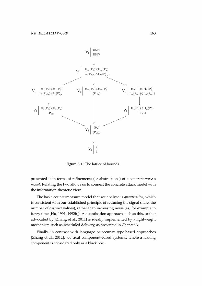
6.4. RELATED WORK 163
V1
∣∣∣∣ UNIV
UNIV
��
V1
∣∣∣∣ H∞(Ps)6H∞(P′s)
L∞(Po|s)6L∞(P′o|s)
vv �� ((
V1
∣∣∣∣ H1(Ps)6H1(P′s)
L1(Po|s)6L1(P′o|s)
��
V1
∣∣∣∣ H∞(Ps)6H∞(P′s)
{Po|s}
��
V1
∣∣∣∣ Hα(Ps)6Hα(P′s)
Lα(Po|s)6Lα(Po|s)
��
V1
∣∣∣∣ H1(Ps)6H1(P′s)
{Po|s}
((
V1
∣∣∣∣ Hα(Ps)6Hα(P′s){Po|s}
vv
V1
∣∣∣∣ {Ps}
{Po|s}
��
V1
∣∣∣∣ ∅∅Figure 6.1: The lattice of bounds.
presented is in terms of refinements (or abstractions) of a concrete processmodel. Relating the two allows us to connect the concrete attack model withthe information-theoretic view.
The basic countermeasure model that we analyse is quantisation, whichis consistent with our established principle of reducing the signal (here, thenumber of distinct values), rather than increasing noise (as, for example infuzzy time [Hu, 1991, 1992b]). A quantisation approach such as this, or thatadvocated by [Zhang et al., 2011] is ideally implemented by a lightweightmechanism such as scheduled delivery, as presented in Chapter 3.
Finally, in contrast with language or security type-based approaches[Zhang et al., 2012], we treat component-based systems, where a leakingcomponent is considered only as a black box.

164 CHAPTER 6. FORMAL LEAKAGE MODELS
6.5 Summary
In this final chapter, we have taken one further step from the details of practicalcountermeasures, and from system verification, and investigated the kindof results that we might expect to be able to verify of a practical system.Remaining within the framework of pGCL, we formalised an operational, orprogrammatic model of the guessing attack of Chapter 2, and demonstratedthat from it we can derive the principal bounds that we previously discussedin information-theoretic terms. This approach thus hints at a bridge betweenthe process-oriented, semantic, view of leakage, and the channel-oriented,information-theoretic view. We took advantage of the fact that the guessing-attack model is not trace-dependent: security can be defined as a predicate onstates, and thus is preserved by refinement, as noted in Section 4.1.
Of particular interest is our rederivation of the notion of min leakagein Equation 6.9, and the connection between the lattice on bounds, and therefinement order in pGCL, as expressed in Figure 6.1. The focus of this chapterwas the establishment of sound information-theoretic bounds on leakage, thatwill survive refinement via the L4.verified proof stack, down to the level ofreal countermeasures, as discussed in Chapter 3 and Chapter 5.
In the preceding three chapters, we have demonstrated that we can builda chain of machine-checked proofs from a concrete probabilistic model (incor-porating a large classical specification, such as seL4), all the way to abstractinformation-theoretic properties of the system modelled as a noisy channel.We thus confirm that the high-level approach we present in Chapter 2 can belinked to a concrete specification, which in turn may apply the countermea-sures discussed in Chapter 3, or a more context-dependent approach, such asthe lattice scheduler verified in Chapter 5.

7 Conclusion
We have surveyed the challenges of provable protection against informationleakage in component-based systems, and contributed both to the under-standing of the low-level mechanisms of leakage, and to the verification ofhigh-level probabilistic properties and countermeasures.
Recognising that while min entropy gives a safe bound on vulnerabil-ity, we have demonstrated that Shannon entropy can lead to simpler, moretractable models (Section 2.5). Our proof (Lemma 4) of the maximum vulnera-bility given Shannon entropy allows such models to be used to safely boundvulnerability, through a pessimistic correction.
The extensive empirical analysis of Chapter 3 covered two local channels(cache and bus contention), and one remote (the lucky thirteen attack onDTLS), and demonstrates the widely varying effectiveness of three mitiga-tion strategies: cache colouring, instruction-based scheduling and scheduleddelivery.
Cache colouring is generally effective against the cache channel, althoughthe capacity of residual channels is increasing on modern hardware, and amore careful implementation is required to avoid compromising artefacts,many of which are only apparent given a large amount of data.
Instruction-based scheduling, which seeks to prevent the use of the pre-emption tick as a clock, has decreased dramatically in effectiveness on recenthardware. On older (circa 2005) ARM processors it is essentially perfect, whileon more recent ARM processors, and on more complex x86 processors it islargely ineffective, with large residual channels apparent. Although applica-ble to a wide range of channels (e.g. bus contention), its performance does notjustify the difficulty of attempting to remove all visible clocks.
The Achilles’ heel of both local-channel countermeasures is their reliance
165

166 CHAPTER 7. CONCLUSION
on unspecified low-level hardware behaviour, which manufacturers are likelyto modify without notice in pursuit of greater performance. It appears that forgenuinely covert-channel-secure systems, partitioned hardware will remainnecessary, although effective mitigation of side-channel leakage, particularlythrough the cache appears to be practical (via colouring).
For the remote channel (lucky thirteen), OS-level techniques allow us toefficiently and effectively mitigate the channel, without requiring any modifi-cation of the vulnerable code in OpenSSL. In fact, we outperform the constant-time implementation in the latest version of the library, both for security andperformance. There is no reason that a more careful implementation shouldnot be able to achieve perfect mitigation at negligible performance cost.
The work presented in Chapter 4 through Chapter 6, demonstrates thatthe refinement-style technique used in L4.verified can be extended to handleprobabilistic properties and probabilistic systems, while incorporating existingproofs. Our formalisation of pGCL in Isabelle/HOL allows us to verify thelattice-lottery scheduler, as an asymptotically fair countermeasure against thecache channel. Finally, we formally derive (with machine-checked proof) theinformation-theoretic bounds introduced in Chapter 2 from a concrete threatmodel: the guessing attack.
We conclude that a significant amount of work remains before we willbe able to formally verify the total absence of timing channels in a systemimplemented on commodity hardware. Nevertheless, we have demonstratedthat effective mitigations do exist for some channels, and that there is nobarrier in principle to verifying such stochastic high-level properties.
A Detailed Proofs
This appendix presents the detailed proofs of several results from Chapter 2,including the extension of the vulnerability divergence result, Lemma 4 ofSection 2.5, to the full class of Rényi entropies [Rényi, 1961], of which theShannon entropy is a special case.
Proof of Lemma 1
Let X be a random variable, ranging over the integers [1,n]. For any fixedy ∈ R, then over all distributions where E(X) = y, E(1/X) is maximised whenall probability mass is assigned either to 1 or to n.
The result is trivial for n 6 2, therefore assume 3 6 n. Fix a distributionP such that EP(X) = y, and assume that EP(1/X) is maximal among suchdistributions. Further assume that for some x ∈ [2,n− 1], P(x) > 0. Let:
α =n− x
n− 1β =
x− 1n− 1
n.b. α+ nβ = x (A.1)
Construct a modified distribution P′ where:
P′(z) =
P(z) + αP(x) z = 1
0 z = x
P(z) + βP(x) z = n
P(z) otherwise
We have redistributed the probability that had been assigned to x between 1
167

168 APPENDIX A. DETAILED PROOFS
and n. Calculating EP′(X) we see that
EP′(X) =∑z
zP′(z)
= [P(1) + αP(x)] + 0 + [n(P(n) + βP(x))] +∑
z∈[2,n−1]−x
zP(z)
= αP(x) + nβP(x) +∑
z∈[1,n]−x
zP(z)
= xP(x) +∑
z∈[1,n]−x
zP(z) By Equation A.1
= EP(X)
Also,
EP′(1/X) =∑z
P′(z)
z
= [P(1) + αP(x)] + 0 +
[P(n) + βP(x)
n
]+
∑z∈[2,n−1]−x
P(z)
z
= (α+β
n)P(x) +
∑z∈[1,n]−x
P(z)
z
> EP(1/X) if α+β
n>
1x
(A.2)
It remains only to show that the inequality in Equation A.2 holds i.e. that wehave strictly increased the value of EP′(1/X):
n+ x < nx as 3 6 n, 2 6 x
∴ (n+ x)(n− x) < nx(n− x) as x < n
∴ (n+ x)(n− x) < nx(n− x) + n− x "
∴ 0 < n2x− nx2 − n2 + x2 + n− x
also
n < n2 as 3 6 n
∴ 0 < n2x− nx as 2 6 x

169
and thus
0 <n2x− nx2 + x2 − x+ n2 − n
n2x− nx
=n− x
n− 1+x− 1n2 − n
−1x
= α+β
n−
1x
finally therefore
α+β
n>
1x
This contradicts the assumption of maximality. Therefore, any distributionthat maximises E(1/X) only assigns probability to 1 and n.
Proof of Lemma 4
Let
Q = {P : H1(P) = H}
be the set of distributions over Xwith Shannon entropyH, and for each P ∈ Q,take any disjoint partition of X as Y ∪ Z such that
∀y ∈ Y, z ∈ Z. y > z∧ |Y| = n
Then, for H > log2|Y|, P(Y) is maximised over Q at the ‘corner point’,where ∀y. P(y) = 1/|Y| and ∀z. P(z) = 1/|Z|.
For H < log2|Y|, a solution exists with P(Y) = 1 and P(X) = 0.The partition of X induces a partition of P:
P(x) =
{P(Y) ∗ PY(x) x ∈ Y
(1 − P(Y)) ∗ PZ(x) x ∈ Zwhere PS(x) =
P(x)
P(S)
Let N = |X|, hence |Z| = N− n. Also, let p = P(Y).The question is: for a given H and n, what is the largest possible p, over
all choices for P? Or, what is the largest probability we can assign to the nmost likely events, and still achieve overall entropy H?
Note that:
H1(PX) = h(p) + pH1(PY) + (1 − p)H1(PZ) (A.3)

170 APPENDIX A. DETAILED PROOFS
where
h(p) = −p log2(p) − (1 − p) log2(1 − p) and 0 log2 0 = 0
and that
0 6 H1(PX) 6 log2N
0 6 H1(PY) 6 log2 n
and 0 6 H1(PZ) 6 log2(N− n)
If H 6 log2 n, a solution exists with H(Y) = H, p = 1. Assume now that:
H > log2 n (A.4)
We rewrite equation Equation A.3 as:
H(Z) =H− h(p)
1 − p−
p
1 − pH(Y) (A.5)
For a given p, the solutions form a line in the H(Y)–H(Z) plane with slopebetween 0 at p = 0, and −∞ at p = 1. What is the greatest p such that this lineintersects the rectangle (0, 0)–(log2 n, log2(N− n))?
As the slope is uniformly non-positive, a solution exists exactly when oneexists on the line:
H(Y)
log2 n=
H(Z)
log2(N− n)(A.6)
Reparameterising and substituting into Equation A.3:
H = h(p) + pk log2 n+ (1 − p)k log2(N− n) (A.7)
k(p) = k =H− h(p)
p log2 n+ (1 − p) log2(N− n)(A.8)
We now need the greatest p such that k(p) ∈ [0, 1]. Note that
k(1) =H
log2(n)(A.9)
> 1 by Equation A.4 (A.10)
Assume that for some q ∈ [0, 1], k(q) 6 1. As k(1) > 1, by the continuity ofk, there exist finitely many q′ ∈ [q, 1] with k(q′) = 1. Let r be the greatestsuch. Again by continuity, @q ′ > q. k(q ′) 6 1. Thus the largest value of p(r) is found when k(p) = 1 i.e. when H(Y) and H(Z) attain their maximumvalues: log2 n and log2(N− n). This occurs only for the uniform distributionsPX(x) =
1n and PY(y) = 1
N−n .

171
Vulnerability given Rènyi Entropy
Definition 7: The Rényi α-entropy of the distribution P over the set X is:
Hα(P) = lima→α
(1
1 − alog2
∑x∈X
P(x)a
)
This subsumes both the Shannon entropy, when α = 1, and the min-entropy, when α =∞. Thus the divergence of H1 is covered by Lemma 4, andthat of H∞ is trivial.
Lemma 16: For α 6= 1, let
Q = {P : Hα(P) = H}
be the set of distributions over X with Renyi α-entropy H, and for each P ∈ Q,partition X disjointly as Y + Z such that
∀y ∈ Y, z ∈ Z. y > z .
For H > log2|Y|, P(Y) is maximised over Q at the ‘corner point’, where∀y. P(y) = 1/|Y| and ∀z. P(z) = 1/|Z|.
For H < log2|Y|, a solution exists with P(Y) = 1 and P(X) = 0.
Proof. The proof is analogous to that of Lemma 4.The partition of X induces a partition of P:
P(x) =
{p ∗ PY(x) x ∈ Y
(1 − p) ∗ PZ(x) x ∈ Zwhere PS(x) =
P(x)
P(S)
Let n = |Y|, N = |X|; hence |Z| = N− n.Let:
Hα(X) =1
1 − αlog2
∑x∈X
P(x)α (A.11)
and define Hα(Y) and Hα(Z) analogously.Note that
0 6 Hα(X) 6 log2N
0 6 Hα(Y) 6 log2 n
0 6 Hα(Z) 6 log2(N− n)

172 APPENDIX A. DETAILED PROOFS
Expanding Equation A.11 and rearranging:
Hα(X) =1
1 − αlog2
∑y∈Y
[pPY(y)]α +∑z∈Z
[(1 − p)PZ(z)]α
=
11 − α
log2
pα∑y∈Y
PY(y)α + (1 − p)α
∑z∈Z
PZ(z)α
=
11 − α
log2
[pα2(1−α)Hα(Y) + (1 − p)α2(1−α)Hα(Z)
]2(1−α)Hα(X) = pα2(1−α)Hα(Y) + (1 − p)α2(1−α)Hα(Z)
As for Shannon entropy, if Hα(X) 6 log2 n, we find a solution with p = 1and Hα(Y) = Hα(X). Therefore, assume:
Hα(X) > log2 n (A.12)
Let:
A = 2(1−α)Hα(X)
B = 2(1−α)Hα(Y) (A.13)
C = 2(1−α)Hα(Z) (A.14)
For α 6= 1, equations Equation A.13 and Equation A.14 give a continuous,invertible change of variables. Thus, it is sufficient to solve the following:
A = pαB+ (1 − p)αC (A.15)
As in Equation A.5, we again have a line of negative slope, this time in theB− C plane.
There are two cases to consider: for α < 1,
n1−α 6 A 6 N1−α
1 6 B 6 n1−α
1 6 C 6 (N− n)1−α
and for α > 1,
N1−α 6 A 6 n1−α
n1−α 6 B 6 1
(N− n)1−α 6 C 6 1

173
Again we reparameterise, looking for solutions on the diagonal:
C = pα(1 + k(n1−α − 1)) + (1 − p)α(1 + k((N− n)1−α − 1))
k(p) =C− pα − (1 − p)α
pα(n1−α − 1) + (1 − p)α((N− n)1−α − 1)(A.16)
Equation A.16 is continuous for p ∈ [0, 1] and n ∈ [0,N] and N > 2. Also:
k(1) =C− 1
n1−α − 1
=2(1−α)Hα(X) − 12(1−α)log2n − 1
> 1 by ass. A.12
Thus the solution that maximises p will again be found at the extremepoint of the rectangle, namely B = n1−α, C = (N− n)1−α. Substituting intoEquation A.15 gives:
2(1−α)Hα(X) = pαn1−α + (1 − p)α(N− n)1−α
Hα(X) =1
1 − αlog2
[pαn1−α + (1 − p)α(N− n)1−α]


Bibliography
Nadhem J. AlFardan and Kenneth G. Paterson. Lucky thirteen: Breaking theTLS and DTLS record protocols. In Proceedings of the IEEE Symposium onSecurity and Privacy, pages 526–540, San Francisco, CA, May 2013. IEEE.doi:10.1109/SP.2013.42.
Mário S. Alvim, Kostas Chatzikokolakis, Catuscia Palamidessi, and GeoffreySmith. Measuring information leakage using generalized gain functions. InProceedings of the 25th IEEE Computer Security Foundations Symposium, pages265–279. IEEE, 2012. doi:10.1109/CSF.2012.26.
Miguel E. Andrés, Catuscia Palamidessi, Peter Rossum, and Geoffrey Smith.Computing the leakage of information-hiding systems. In Javier Esparzaand Rupak Majumdar, editors, Proceedings of the 16th International Conferenceon Tools and Algorithms for the Construction and Analysis of Systems (TACAS),volume 6015 of Lecture Notes in Computer Science, pages 373–389. Springer,2010. doi:10.1007/978-3-642-12002-2_32.
Suguru Arimoto. An algorithm for computing the capacity of arbitrary discretememoryless channels. IEEE Transactions on Information Theory, 18(1):14–20,1972. doi:10.1109/TIT.1972.1054753.
Cortex A9 TRM. Cortex-A9 (revision r3p0) Technical Reference Manual. ARMLtd., July 2011.
Ross Arnold and Tim Bell. A corpus for the evaluation of lossless compressionalgorithms. In Proceedings of the 1997 Data Compression Conference, pages201–210. IEEE, 1997. doi:10.1109/DCC.1997.582019.
Aslan Askarov, Andrew C. Myers, and Danfeng Zhang. Predictive black-boxmitigation of timing channels. In Proceedings of the 17th ACM Conferenceon Computer and Communications Security, pages 520–538, Chicago, Illinois,USA, 2010. ACM. doi:10.1145/1866307.1866341.
175

176 BIBLIOGRAPHY
Amittai Aviram, Sen Hu, Bryan Ford, and Ramakrishna Gummadi. Determi-nating timing channels in compute clouds. In Proceedings of the 2010 ACMWorkshop on Cloud Computing Security, pages 103–108, Chicago, Illinois, USA,2010a. ACM. doi:10.1145/1866835.1866854.
Amittai Aviram, Shu-Chun Weng, Sen Hu, and Bryan Ford. Efficient system-enforced deterministic parallelism. In Proceedings of the 9th USENIX Sympo-sium on Operating Systems Design and Implementation, Vancouver, BC, 2010b.USENIX.
Michael Backes, Markus Dürmuth, Sebastian Gerling, Manfred Pinkal, andCaroline Sporleder. Acoustic side-channel attacks on printers. In Proceedingsof the 19th USENIX Security Symposium, pages 1–16, Washington, DC, 2010.USENIX.
Christel Baier and Marta Kwiatkowska. Automatic verification of livenessproperties of randomized systems. In Proceedings of the 16th ACM Symposiumon Principles of Distributed Computing, page 295. ACM, 1997. doi:10.1145/259380.259527.
Gilles Barthe, Benjamin Grégoire, and Santiago Zanella Béguelin. Formalcertification of code-based cryptographic proofs. In Proceedings of the 36thACM SIGPLAN-SIGACT Symposium on Principles of Programming Languages,pages 90–101, Savannah, GA, USA, 2009. ACM. doi:10.1145/1480881.
1480894. URL http://doi.acm.org/10.1145/1480881.1480894.
Gilles Barthe, Benjamin Grégoire, Sylvain Heraud, and Santiago ZanellaBéguelin. Computer-aided security proofs for the working cryptographer. InPhillip Rogaway, editor, Advances in Cryptology – CRYPTO 2011, volume 6841of Lecture Notes in Computer Science, pages 71–90. Springer Berlin Heidelberg,2011. ISBN 978-3-642-22791-2. doi:10.1007/978-3-642-22792-9_5. URLhttp://dx.doi.org/10.1007/978-3-642-22792-9_5.
Gilles Barthe, Gustavo Betarte, Juan Diego Campo, and Carlos Luna. Cache-leakage resilient OS isolation in an idealized model of virtualization. InProceedings of the 25th IEEE Computer Security Foundations Symposium, pages186–197. IEEE, 2012a. doi:10.1109/CSF.2012.17.
Gilles Barthe, Boris Köpf, Federico Olmedo, and Santiago Zanella Béguelin.Probabilistic relational reasoning for differential privacy. In Proceedings of the

BIBLIOGRAPHY 177
39th ACM SIGPLAN-SIGACT Symposium on Principles of Programming Lan-guages, pages 97–110, Philadelphia, PA, USA, 2012b. ACM. doi:10.1145/2103656.2103670. URL http://doi.acm.org/10.1145/2103656.2103670.
Gertrud Bauer and Markus Wenzel. Calculational reasoning revisited – anIsabelle/Isar experience. In Proceedings of the 14th International Conference onTheorem Proving in Higher Order Logics, pages 75–90. Springer, 2001.
Tom Bergan, Nicholas Hunt, Luis Ceze, and Steven D. Gribble. Deterministicprocess groups in dOS. In Proceedings of the 9th USENIX Symposium onOperating Systems Design and Implementation, pages 1–16, Vancouver, BC,Canada, 2010. USENIX.
Richard E. Blahut. Computation of channel capacity and rate-distortionfunctions. IEEE Transactions on Information Theory, 18:460–473, 1972. doi:10.1.1.133.7174.
Christelle Braun, Konstantinos Chatzikokolakis, and Catuscia Palamidessi.Quantitative notions of leakage for one-try attacks. Electronic Notes inTheoretical Computer Science, 249:75–91, August 2009. doi:10.1016/j.entcs.2009.07.085.
David Brumley and Dan Boneh. Remote timing attacks are practical. InProceedings of the 12th USENIX Security Symposium, pages 1–14, Washington,DC, USA, 2003. USENIX. doi:10.1016/j.comnet.2005.01.010.
Lewis Carroll. Alice’s Adventures in Wonderland. Macmillan, November 1865.
Han Chen and Pasquale Malacaria. Quantitative analysis of leakage for multi-threaded programs. In Proceedings of the 2007 ACM SIGPLAN Workshop onProgramming Languages and Analysis for Security, pages 31–40, San Diego,California, USA, 2007. ACM. doi:10.1145/1255329.1255335.
Michael R. Clarkson, Andrew C. Myers, and Fred B. Schneider. Belief in infor-mation flow. In Proceedings of the 18th IEEE Computer Security FoundationsWorkshop, pages 31–45. IEEE, June 2005. doi:10.1109/CSFW.2005.10.
Aaron R. Coble. Anonymity, information, and machine-assisted proof. PhD thesis,University of Cambridge, Computer Laboratory, 2010.

178 BIBLIOGRAPHY
David Cock. Bitfields and tagged unions in C: Verification through automaticgeneration. In Bernhard Beckert and Gerwin Klein, editors, Proceedings ofthe 5th International Verification Workshop, volume 372 of CEUR WorkshopProceedings, pages 44–55, Sydney, Australia, August 2008.
David Cock. Lyrebird – assigning meanings to machines. In Gerwin Klein, RalfHuuck, and Bastian Schlich, editors, Proceedings of the 5th Systems SoftwareVerification, pages 1–9, Vancouver, Canada, October 2010. USENIX.
David Cock. Exploitation as an inference problem. In Proceedings of the 4thACM Workshop on Artificial Intelligence and Security, pages 105–106, Chicago,IL, USA, October 2011. ACM. doi:10.1145/2046684.2046702.
David Cock. Verifying probabilistic correctness in Isabelle with pGCL. In Pro-ceedings of the 7th Systems Software Verification, pages 1–10, Sydney, Australia,November 2012. Electronic Proceedings in Theoretical Computer Science.doi:10.4204/EPTCS.102.15.
David Cock. Practical probability: Applying pGCL to lattice schedul-ing. In Proceedings of the 4th International Conference on Interactive TheoremProving, pages 1–16, Rennes, France, July 2013. Springer. doi:10.1007/
978-3-642-39634-2_23.
David Cock. From probabilistic operational semantics to information theory;side channels in pGCL with isabelle. In Proceedings of the 5th InternationalConference on Interactive Theorem Proving, pages 1–15, Vienna, Austria, July2014. Springer. doi:10.1007/978-3-319-08970-6_12.
David Cock, Gerwin Klein, and Thomas Sewell. Secure microkernels, statemonads and scalable refinement. In Otmane Ait Mohamed, César Mu noz,and Sofiène Tahar, editors, Proceedings of the 21st International Conference onTheorem Proving in Higher Order Logics, pages 167–182, Montreal, Canada,August 2008. Springer. doi:10.1007/978-3-540-71067-7_16.
David Cock, Qian Ge, Toby Murray, and Gernot Heiser. The last mile; anempirical study of timing channels on sel4. In Proceedings of the 21st ACMConference on Computer and Communications Security, pages 1–12, Scottsdale,USA, November 2014. ACM. doi:10.1145/2660267.2660294. (to appear).

BIBLIOGRAPHY 179
Cryptome. How old is TEMPEST?, 2002. URL http://cryptome.org/
tempest-old.htm. Accessed 11 March 2014.
Matthias Daum, Nelson Billing, and Gerwin Klein. Concerned with the un-privileged: User programs in kernel refinement. Formal Aspects of Computing.doi:10.1007/s00165-014-0296-9. (to appear).
Matteo Dell’Amico, Pietro Michiardi, and Yves Roudier. Password strength:An empirical analysis. In Proceedings of the 30th IEEE INFOCOM, pages 1–9.IEEE, 2010. doi:10.1109/INFCOM.2010.5461951.
Dorothy. E. Denning. A lattice model of secure information flow. Communica-tions of the ACM, 19:236–242, 1976. doi:10.1145/360051.360056.
Philip Derrin, Kevin Elphinstone, Gerwin Klein, David Cock, and ManuelM. T. Chakravarty. Running the manual: An approach to high-assurancemicrokernel development. In Proceedings of the ACM SIGPLAN Haskell Work-shop, Portland, OR, USA, September 2006. ACM. doi:10.1145/1159842.
1159850.
Edsger W. Dijkstra. Guarded commands, nondeterminacy and formal deriva-tion of programs. Communications of the ACM, 18(8):453–457, August 1975.doi:10.1145/360933.360975.
Adam Dunkels. Minimal TCP/IP implementation with proxy support. Tech-nical Report T2001-20, SICS, 26, 2001. http://www.sics.se/~adam/thesis.pdf.
Dhammika Elkaduwe, Gerwin Klein, and Kevin Elphinstone. Verified pro-tection model of the seL4 microkernel. In Jim Woodcock and NatarajanShankar, editors, Proceedings of Verified Software: Theories, Tools and Experi-ments 2008, volume 5295 of Lecture Notes in Computer Science, pages 99–114,Toronto, Canada, October 2008. Springer.
Barbara Espinoza and Geoffrey Smith. Min-entropy leakage of channelsin cascade. In Gilles Barthe, Anupam Datta, and Sandro Etalle, editors,Proceedings of the 10th International Workshop on Formal Aspect of Security andTrust (FAST), volume 7140 of Lecture Notes in Computer Science, pages 70–84.Springer, 2012. doi:10.1007/978-3-642-29420-4_5.

180 BIBLIOGRAPHY
Barbara Espinoza and Geoffrey Smith. Min-entropy as a resource. Informationand Computation, 226:57–75, 2013. doi:10.1016/j.ic.2013.03.005.
Colin Fidge and Carron Shankland. But what if i don’t want to wait for-ever? Formal Aspects of Computing, 14:281–294, 2003. doi:10.1007/
s001650300006.
Bryan Ford. Plugging side-channel leaks with timing information flow control.In Proceedings of the 4th USENIX Workschop on Hot Topics in Cloud Computing,pages 1–5, Boston, MA, 2012. USENIX.
Richard Gay, Heiko Mantel, and Henning Sudbrock. Empirical bandwidthanalysis of interrupt-related covert channels. In Proceedings of the 2nd In-ternational Workshop on Quantitative Aspects in Security Assurance, London,September 2013.
Michael Godfrey. On the prevention of cache-based side-channel attacks in acloud environment. Master’s thesis, Queen’s University, Ontario, Canada,September 2013. doi:1974/8320.
Joseph Goguen and José Meseguer. Security policies and security models.In Proceedings of the IEEE Symposium on Security and Privacy, pages 11–20,Oakland, California, USA, April 1982. IEEE Computer Society.
Xun Gong, Negar Kiyavash, and Parv Venkitasubramaniam. Informationtheoretic analysis of side channel information leakage in FCFS schedulers.In Proceedings of the 2011 IEEE International Symposium on Information Theory,pages 1255–1259. IEEE, August 2011. doi:10.1109/ISIT.2011.6033737.
James W. Gray. Probabilistic interference. In Proceedings of the 1990 IEEEComputer Society Symposium on Research in Security and Privacy, pages 170–179, May 1990. doi:10.1109/RISP.1990.63848.
James W. Gray. On introducing noise into the bus-contention channel. InProceedings of the IEEE Symposium on Security and Privacy, pages 90–98. IEEEComputer Society, 1993. doi:10.1109/RISP.1993.287640.
James W. Gray. Countermeasures and tradeoffs for a class of covert timingchannels. Technical Report HKUST-CS94-18, Hong Kong University ofScience and Technology, 1994. doi:1783.1/25.

BIBLIOGRAPHY 181
Friedrich Gretz, Joost-Pieter Katoen, and Annabelle McIver. Operationalversus weakest pre-expectation semantics for the probabilistic guardedcommand language. Performance Evaluation, 73(0):110–132, 2014. doi:10.1016/j.peva.2013.11.004.
David Greve and Matthew Wilding. Evaluatable, high-assurance microproces-sors. In Proceedings of the 2nd Annual High-Confidence Software and SystemsConference, Annapolis, MD, USA, 2002.
W.R. Harris, S. Jha, T. Reps, J. Anderson, and R.N.M. Watson. Declarative,temporal, and practical programming with capabilities. In Proceedingsof the IEEE Symposium on Security and Privacy, pages 18–32, May 2013.doi:10.1109/SP.2013.11.
William L. Harrison and Richard B. Kieburtz. The logic of demand in Haskell.Journal of Functional Programming, 15(6):837–891, November 2005. doi:
10.1017/S0956796805005666.
Johannes Hölzl and Tobias Nipkow. Verifying pCTL model checking. InCormac Flanagan and Barbara König, editors, Proceedings of the 18th Interna-tional Conference on Tools and Algorithms for the Construction and Analysis ofSystems (TACAS), volume 7214 of Lecture Notes in Computer Science, pages347–361. Springer, 2012. doi:10.1007/978-3-642-28756-5_24.
Wei-Ming Hu. Reducing timing channels with fuzzy time. In Proceedings ofthe 1991 IEEE Computer Society Symposium on Research in Security and Privacy,pages 8–20. IEEE Computer Society, 1991. doi:10.1109/RISP.1991.130768.
Wei-Ming Hu. Lattice scheduling and covert channels. In Proceedings ofthe IEEE Symposium on Security and Privacy, pages 52–61. IEEE, 1992a.doi:10.1109/RISP.1992.213271.
Wei-Ming Hu. Reducing timing channels with fuzzy time. Journal of ComputerSecurity, 1(3–4), January 1992b. doi:10.3233/JCS-1992-13-404.
Brian Huffman. Formal verification of monad transformers. In Proceedingsof the 17th International Conference on Functional Programming, pages 15–16,Copenhagen, Denmark, 2012. ACM. doi:10.1145/2364527.2364532.

182 BIBLIOGRAPHY
Marieke Huisman and Tri Minh Ngo. Scheduler-specific confidentialityfor multi-threaded programs and its logic-based verification. In Proceed-ings of the 2011 International Conference on Formal Verification of Object-Oriented Software, pages 178–195, Turin, Italy, 2012. Springer. doi:10.1007/978-3-642-31762-0_12.
Joe Hurd, Annabelle McIver, and Carroll Morgan. Probabilistic guardedcommands mechanized in HOL. Theoretical Computer Science, 346(1):96 –112, 2005. doi:10.1016/j.tcs.2005.08.005.
Intel 64 & IA-32 AORM. Intel 64 and IA-32 Architectures Optimization ReferenceManual. Intel Corporation, April 2012.
Paul A. Karger and John C. Wray. Storage channels in disk arm optimization.In Proceedings of the 1991 IEEE Computer Society Symposium on Research inSecurity and Privacy, pages 52–61. IEEE Computer Society, May 1991.doi:10.1109/RISP.1991.130771.
Paul A. Karger, Mary Ellen Zurko, Douglas W. Bonin, Andrew H. Mason,and Clifford E. Kahn. A retrospective on the VAX VMM security kernel.IEEE Transactions on Software Engineering, 17(11):1147–1165, November 1991.doi:10.1109/32.106971.
Richard A. Kemmerer. Shared resource matrix methodology: an approachto identifying storage and timing channels. ACM Transactions on ComputerSystems, 1(3):256–277, August 1983. doi:10.1145/357369.357374.
Richard A. Kemmerer. A practical approach to identifying storage and timingchannels: twenty years later. In Proceedings of the 19th Annual ComputerSecurity Applications Conference (ACSAC), pages 109–118. IEEE, December2002. doi:10.1109/CSAC.2002.1176284.
Taesoo Kim, Marcus Peinado, and Gloria Mainar-Ruiz. STEALTHMEM: system-level protection against cache-based side channel attacks in the cloud. InProceedings of the 21st USENIX Security Symposium, pages 189–204, Bellevue,WA, USA, August 2012. USENIX.
Gerwin Klein, Kevin Elphinstone, Gernot Heiser, June Andronick, DavidCock, Philip Derrin, Dhammika Elkaduwe, Kai Engelhardt, Rafal Kolanski,Michael Norrish, Thomas Sewell, Harvey Tuch, and Simon Winwood. seL4:

BIBLIOGRAPHY 183
Formal verification of an OS kernel. In Proceedings of the 22nd ACM Sym-posium on Operating Systems Principles, pages 207–220, Big Sky, MT, USA,October 2009. ACM. doi:10.1145/1629575.1629596.
Gerwin Klein, June Andronick, Kevin Elphinstone, Gernot Heiser, DavidCock, Philip Derrin, Dhammika Elkaduwe, Kai Engelhardt, Rafal Kolanski,Michael Norrish, Thomas Sewell, Harvey Tuch, and Simon Winwood. seL4:Formal verification of an operating system kernel. Communications of theACM, 53(6):107–115, June 2010. doi:10.1145/1743546.1743574.
Gerwin Klein, June Andronick, Kevin Elphinstone, Toby Murray, ThomasSewell, Rafal Kolanski, and Gernot Heiser. Comprehensive formal verifi-cation of an OS microkernel. ACM Transactions on Computer Systems, 32(1):2:1–2:70, February 2014. doi:10.1145/2560537.
Paul Kocher, Joshua Jaffe, and Benjamin Jun. Differential power analysis.In Michael Wiener, editor, Advances in Cryptology – CRYPTO ’99, volume1666 of Lecture Notes in Computer Science, pages 388–397. Springer, 1999.doi:10.1007/3-540-48405-1_25.
Boris Köpf and David Basin. An information-theoretic model for adaptiveside-channel attacks. In Proceedings of the 14th ACM Conference on Computerand Communications Security, pages 286–296, Alexandria, Virginia, USA,2007. ACM. doi:10.1145/1315245.1315282.
Boris Köpf and Geoffrey Smith. Vulnerability bounds and leakage resilienceof blinded cryptography under timing attacks. In Proceedings of the 23rdIEEE Computer Security Foundations Symposium, pages 44–56, Washington,DC, USA, 2010. IEEE Computer Society. doi:10.1109/CSF.2010.11.
Dexter Kozen. A probabilistic PDL. Journal of Computer and System Sciences, 30(2):162–178, 1985. doi:10.1016/0022-0000(85)90012-1.
Butler W. Lampson. A note on the confinement problem. Communications ofthe ACM, 16:613–615, 1973. doi:10.1145/362375.362389.
Jochen Liedtke, Hermann Härtig, and Michael Hohmuth. OS-controlled cachepredictability for real-time systems. In Proceedings of the 3rd IEEE Real-TimeTechnology and Applications Symposium (RTAS), Montreal, Canada, June 1997.IEEE. doi:10.1109/RTTAS.1997.601360.

184 BIBLIOGRAPHY
Steven. B. Lipner. A comment on the confinement problem. In Proceedingsof the 5th ACM Symposium on Operating Systems Principles, pages 192–196.ACM, 1975. doi:10.1145/800213.806537.
David Malone and Kevin Maher. Investigating the distribution of passwordchoices. In Proceedings of the 21st international conference on World Wide Web,WWW ’12, pages 301–310, Lyon, France, 2012. ACM. doi:10.1145/2187836.2187878.
James L. Massey. Guessing and entropy. In Proceedings of the 1994 IEEEInternational Symposium on Information Theory, page 204. IEEE, June 1994.doi:10.1109/ISIT.1994.394764.
Daniel Matichuk and Toby Murray. Extensible specifications for automaticre-use of specifications and proofs. In Proceedings of the 10th International Con-ference on Software Engineering and Formal Methods, pages 1–8, Thessaloniki,Greece, December 2012. Springer. doi:10.1007/978-3-642-33826-7_23.
Annabelle McIver and Carroll Morgan. Partial correctness for probabilisticdemonic programs. Theoretical Computer Science, 266(1-2):513 – 541, 2001.doi:10.1016/S0304-3975(00)00208-5.
Annabelle McIver and Carroll Morgan. Abstraction, Refinement and Prooffor Probabilistic Systems. Springer, 2004. ISBN 978-0-387-40115-7. doi:
10.1007/b138392.
Carroll Morgan and Annabelle K. McIver. An expectation-based model forprobabilistic temporal logic. Logic Journal of the IGPL, 7:779–804, 1999.doi:10.1093/jigpal/7.6.779.
Carroll Morgan, Annabelle McIver, Geoffrey Smith, Barbara Espinoza, andLarisa Meinicke. Abstract channels and their robust information-leakageordering. In Principles of Security and Trust (ETAPS), pages 83–102, Grenoble,France, April 2014.
Till Mossakowski, Lutz Schröder, and Sergey Goncharov. A generic completedynamic logic for reasoning about purity and effects. Formal Aspects ofComputing, 22(3-4):363–384, May 2010. doi:10.1007/s00165-010-0153-4.
Steven J. Murdoch. Hot or not: revealing hidden services by their clock skew.In Proceedings of the 13th ACM Conference on Computer and Communications

BIBLIOGRAPHY 185
Security, pages 27–36, Alexandria, Virginia, USA, 2006. ACM. doi:10.1145/1180405.1180410.
Toby Murray, Daniel Matichuk, Matthew Brassil, Peter Gammie, and GerwinKlein. Noninterference for operating system kernels. In Chris Hawblitzeland Dale Miller, editors, Proceedings of the 2nd International Conference onCertified Programs and Proofs, volume 7679 of Lecture Notes in ComputerScience, pages 126–142, Kyoto, Japan, December 2012. Springer. doi:10.
1007/978-3-642-35308-6_12.
Toby Murray, Daniel Matichuk, Matthew Brassil, Peter Gammie, TimothyBourke, Sean Seefried, Corey Lewis, Xin Gao, and Gerwin Klein. seL4: fromgeneral purpose to a proof of information flow enforcement. In Proceedingsof the IEEE Symposium on Security and Privacy, pages 415–429, San Francisco,CA, USA, May 2013. IEEE. doi:10.1109/SP.2013.35.
Tobias Nipkow. Hoare logics in Isabelle/HOL. In H. Schwichtenberg andR. Steinbrüggen, editors, Proof and System-Reliability, pages 341–367. Kluwer,2002. doi:10.1007/978-94-010-0413-8_11.
Tobias Nipkow, Lawrence Paulson, and Markus Wenzel. Isabelle/HOL —A Proof Assistant for Higher-Order Logic, volume 2283 of Lecture Notes inComputer Science. Springer, 2002. ISBN 978-3-540-43376-7. doi:10.1007/
3-540-45949-9.
NSA. TEMPEST: A signal problem. Cryptologic Spectrum, September 1972.Declassified 2007.
Alfréd Rényi. On measures of entropy and information. In Proceedings of theFourth Berkeley Symposium on Mathematical Statistics and Probability, pages547–561, 1961.
Thomas Ristenpart, Eran Tromer, Hovav Shacham, and Stefan Savage. Hey,you, get off of my cloud: exploring information leakage in third-partycompute clouds. In Proceedings of the 16th ACM Conference on Computer andCommunications Security, pages 199–212, Chicago, IL, USA, 2009. ACM.doi:10.1145/1653662.1653687.
Ronald L. Rivest, Adi Shamir, and Leonard Adleman. A method for obtainingdigital signatures and public-key cryptosystems. Communications of theACM, 21:120–126, 1978. doi:10.1145/359340.359342.

186 BIBLIOGRAPHY
Marvin Schaefer, Barry Gold, Richard Linde, and John Scheid. Programconfinement in KVM/370. In Proceedings of the 5th ACM Computer ScienceConference, pages 404–410, Atlanta, GA, USA, 1977. ACM. doi:10.1145/
800179.1124633.
Steve Selvin. A problem in probability (letter to the editor). American Statisti-cian, 29(1):67, February 1975.
Claude E. Shannon. A mathematical theory of communication. The BellSystem Technical Journal, 1948. doi:10.1145/584091.584093. Reprinted inSIGMOBILE Mobile Computing and Communications Review, 5(1):3–55,2001.
Olin Sibert, Phillip A Porras, and Robert Lindell. The Intel 80x86 processorarchitecture: Pitfalls for secure systems. In Proceedings of the IEEE Symposiumon Security and Privacy. IEEE, 1995. doi:10.1.1.17.5041.
Geoffrey Smith. On the foundations of quantitative information flow. InProceedings of the 12th International Conference on Foundations of SoftwareScience and Computational Structures, pages 288–302, York, UK, 2009. Springer.doi:10.1007/978-3-642-00596-1_21.
Deian Stefan, Pablo Buiras, Edward Z. Yang, Amit Levy, David Terei, Ale-jandro Russo, and David Mazières. Eliminating cache-based timing at-tacks with instruction-based scheduling. In Proceedings of the 18th EuropeanSymposium On Research in Computer Security, pages 718–735, Egham, UK,September 2013. Springer. doi:10.1007/978-3-642-40203-6_40.
David Tam, Reza Azimi, Livio Soares, and Michael Stumm. Managing sharedL2 caches on multicore systems in software. In Proceedings of the 3rd Workshopon the Interaction between Operating Systems and Computer Architecture, SanDiego, CA, USA, June 2007.
Jonathan T. Trostle. Modelling a fuzzy time system. In Proceedings of the 1993IEEE Computer Society Symposium on Research in Security and Privacy, pages82–89. IEEE Computer Society, 1993. doi:10.1109/RISP.1993.287641.
DoD. Trusted Computer System Evaluation Criteria. US Department of Defence,1986. DoD 5200.28-STD.

BIBLIOGRAPHY 187
NIST. Common Criteria for IT Security Evaluation. US National Institute ofStandards, 1999. ISO Standard 15408. http://csrc.nist.gov/cc/.
Carl A. Waldspurger and William E. Weihl. Lottery scheduling: Flexibleproportional-share resource management. In Proceedings of the 1st USENIXSymposium on Operating Systems Design and Implementation, pages 1–11,Monterey, CA, USA, November 1994. USENIX.
Bryan C. Ward, Jonathan L. Herman, Christopher J. Kenna, and James H.Anderson. Making shared caches more predictable on multicore platforms.In Proceedings of the 25th Euromicro Conference on Real-Time Systems, pages157–167, Paris, France, July 2013. doi:10.1109/ECRTS.2013.26.
Chelsea C. White and Douglas J. White. Markov decision processes. Eu-ropean Journal of Operational Research, 39(1):1–16, 1989. doi:10.1016/
0377-2217(89)90348-2.
Simon Winwood, Gerwin Klein, Thomas Sewell, June Andronick, DavidCock, and Michael Norrish. Mind the gap: A verification framework forlow-level C. In Stefan Berghofer, Tobias Nipkow, Christian Urban, andMakarius Wenzel, editors, Proceedings of the 22nd International Conferenceon Theorem Proving in Higher Order Logics, volume 5674 of Lecture Notes inComputer Science, pages 500–515, Munich, Germany, August 2009. Springer.doi:10.1007/978-3-642-03359-9_34.
John C. Wray. An analysis of covert timing channels. In Proceedings of the 1991IEEE Computer Society Symposium on Research in Security and Privacy, pages2–7. IEEE, May 1991. doi:10.1109/RISP.1991.130767.
Yaming Yu. Squeezing the Arimoto-Blahut algorithm for faster convergence.IEEE Transactions on Information Theory, 56(7):3149–3157, 2010. doi:10.1109/TIT.2010.2048452.
Danfeng Zhang, Aslan Askarov, and Andrew C. Myers. Predictive mitigationof timing channels in interactive systems. In Proceedings of the 18th ACMConference on Computer and Communications Security, pages 563–574, Chicago,IL, USA, 2011. ACM. doi:10.1145/2046707.2046772.
Danfeng Zhang, Aslan Askarov, and Andrew C. Myers. Language-basedcontrol and mitigation of timing channels. In Proceedings of the 2012 ACM

188 BIBLIOGRAPHY
SIGPLAN Conference on Programming Language Design and Implementation,pages 99–110, Beijing, China, 2012. ACM. doi:10.1145/2254064.2254078.
Kehuan Zhang, Zhou Li, Rui Wang, XiaoFeng Wang, and Shuo Chen. Side-buster: Automated detection and quantification of side-channel leaks inweb application development. In Proceedings of the 17th ACM Conference onComputer and Communications Security, pages 595–606, New York, NY, USA,2010. ACM. doi:10.1145/1866307.1866374.