Embed Size (px)
Citation preview

Le, Bryant Linh Hai (2014) Modelling railway bridge asset management. PhD thesis, University of Nottingham.
Access from the University of Nottingham repository: http://eprints.nottingham.ac.uk/14271/1/Thesis_Bryant.pdf
Copyright and reuse:
The Nottingham ePrints service makes this work by researchers of the University of Nottingham available open access under the following conditions.
This article is made available under the University of Nottingham End User licence and may be reused according to the conditions of the licence. For more details see: http://eprints.nottingham.ac.uk/end_user_agreement.pdf
For more information, please contact [email protected]
Modelling Railway Bridge Asset
Management
Bryant Linh Hai Le
A Doctoral Thesis
Thesis submitted to the University of Nottingham for the degree of
Doctor of Philosophy
January 2014


i
Abstract
The UK has a long history in the railway industry with a large
number of railway assets. Railway bridges form one of the major
asset groups with more than 35,000 bridges. The majority of the
bridge population are old being constructed over 100 years ago.
Many of the bridges were not designed to meet the current
network demand. With an expected increasing rate of
deterioration due to the increasing traffic loads and intensities,
the management authorities are faced with the difficult task of
keeping the bridge in an acceptable condition with the constraint
budget and minimum service disruptions. Modelling tools with
higher complexity are required to model the degradation of assets
and the effects of different maintenance strategies, in order to
support the management decision making process.
This research aims to address the deficiencies of the current
bridge condition systems and bridge models reported in the
literature and to demonstrate a complete modelling approach to
bridge asset management. The degradation process of a bridge
element is studied using the historical maintenance data where
previous maintenance actions were triggered by a certain type of
defects. Two bridge models are then developed accounting for the
degradation distributions, service and inspection frequency, repair
delay time and different repair strategies. The models provide a
mean of predicting the asset future condition as well as
investigating the effects of different maintenance strategies will
have on a particular asset. The first model is a continuous-time
Markov bridge model and is considered more complex than other
models in the literature, the model demonstrates the advantages
of the Markov modelling technique as well as highlighting its
limitations. The second bridge model presented a novel Petri-Net
modelling approach to bridge asset modelling. This stochastic
modelling technique allows much more detail modelling of bridge
components, considering: non-constant deterioration rates;
protective coating modelling; limits of the number of repairs can
be carried out; and the flexibility of the model allows easily
extension to the model or the number of components modelled.
By applying the two models on the same asset, a comparison can
be made and the results further confirm the validations and

ii
improvements of the presented Petri-Net approach. Finally,
optimisation technique (Genetic Algorithm) is applied to the
bridge models to find the optimum maintenance strategies in
which the objectives are to minimise the whole life cycle cost
whist maximising the asset average condition. A hybrid
optimisation that takes advantage of both bridge models,
resulting in a significant time saving, is also presented.

iii
Acknowledgements
First and foremost, I would like to express my sincere
appreciation to Professor John Andrews, for the continuous
support throughout my PhD research, for his patience, motivation
and immense knowledge. His guidance has helped me
tremendously in all the time of researching and writing this thesis.
I am extremely grateful to have him as my supervisor and believe
that he is the best supervisor one could have. Special thanks to
Dr Rasa Remenyte-Prescott and Dr Daren Prescott for their help
and advice over the last few years.
I would also like to thank Andy Kirwan for the sponsorship, and
giving me the opportunity to start on this project. His willingness
to support this project is very much appreciated. I wish to thank
Sam Chew and Julian Williams and other members of Network
Rail for their valuable inputs and knowledge throughout the
development of this research.
I would like to extend my thanks to other member of
Infrastructure Asset Management group and the people of the
Nottingham Transportation Engineering Centre for their
assistance, encouragement and friendship. I am very fortunate to
have met all these lovely people. Thanks to Matthew Audley who
has always made my time in the office more fun. Thanks to all
other people in the group who have played cards with me at lunch
time and have made my time more enjoyable.
Finally, I wish to thank my mom, my dad, my brother and his
family, and all my friends for their constant support and
understanding throughout my research. Without them this thesis
would not have been possible.
iv
Publications
Journal articles
LE, B. & ANDREWS, J. 2013. Modelling railway bridge asset management. Proceedings of the Institution of Mechanical
Engineers, Part F: Journal of Rail and Rapid Transit, 227, 644-656.
Conference papers
LE, B. & ANDREWS, J. 2012. Railway bridge asset management
modelling. In Proceedings of Rail Research UK Association Annual (RRUKA) Conference 2012, 7th November, London 2012.
LE, B. & ANDREWS, J. 2013. A Markov modelling approach to
railway bridge asset management. In Proceedings of AR2TS seminar: advances in risk and reliability technology symposium,
Loughborough, United Kingdom, 2013.

v
Abbreviations
ABT Abutment
BGL Bearing
CAF Cost Analysis Framework
CARRS Civil Asset Register and Electronic Reporting System
CECASE Civil Engineering Cost and Strategy Evaluation
CP Control period
CPN Coloured Petri-Net
DCK Deck
G Good condition
GA Genetic Algorithm
GSPN Generalised Stochastic Petri-Nets
LCC Life cycle costs
MGE External Main Girder
MGI Internal Main Girder
MK Markov
MOGA Multi-objective Genetic Algorithm
MONITOR Monitor dataset
MTTF Mean time to failure
MTTR Mean time to repair
N New condition
ORR Office of Rail Regulator
P Poor condition
PN Petri-Net
SCMI Structure Condition Monitoring Index
VERA Structure Assessment Database
VP Very poor condition
WLCC Whole life cycle costs

vi
vii
Table of contents
ABSTRACT ....................................................................................................................................... I
ACKNOWLEDGEMENTS ........................................................................................................... III
PUBLICATIONS ............................................................................................................................ IV
ABBREVIATIONS .......................................................................................................................... V
TABLE OF CONTENTS .............................................................................................................. VII
CHAPTER 1 - INTRODUCTION ............................................................................................ 1
1.1 BACKGROUND AND RESEARCH MOTIVATION ............................................................................. 1 1.2 RESEARCH AIMS AND OBJECTIVES ............................................................................................. 3
1.2.1 Aims .................................................................................................................................. 3 1.2.2 Objectives ......................................................................................................................... 4
1.3 THESIS OUTLINE ........................................................................................................................ 4
CHAPTER 2 - LITERATURE REVIEW ................................................................................ 7
2.1 INTRODUCTION .......................................................................................................................... 7 2.2 FUNDAMENTAL OF MARKOV-BASED MODEL ............................................................................. 8 2.3 MODEL STATES .......................................................................................................................... 9 2.4 TRANSITION PROBABILITY ....................................................................................................... 10 2.5 MARKOV MODEL ..................................................................................................................... 12 2.6 RELIABILITY–BASED MODEL ................................................................................................... 14 2.7 SEMI–MARKOV MODEL ........................................................................................................... 18 2.8 SUMMARY AND DISCUSSION .................................................................................................... 24
CHAPTER 3 - DATA ANALYSIS AND DETERIORATION MODELLING .................. 27
3.1 INTRODUCTION ........................................................................................................................ 27 3.2 DATABASE ............................................................................................................................... 27
3.2.1 Data problems and assumptions ...................................................................................... 30 3.2.2 Bridge types .................................................................................................................... 31 3.2.3 Bridge major elements .................................................................................................... 31
3.3 ELEMENT CONDITION STATES .................................................................................................. 32 3.4 INTERVENTIONS ....................................................................................................................... 33 3.5 DETERIORATION MODELLING .................................................................................................. 34
3.5.1 Life time data .................................................................................................................. 34 3.5.2 Distribution fitting .......................................................................................................... 35 3.5.3 Estimation method .......................................................................................................... 36 3.5.4 Expert estimation ............................................................................................................ 37 3.5.5 Single component degradation rate estimation ............................................................... 37
3.6 RESULTS AND DISCUSSIONS .................................................................................................... 38 3.6.1 Component degradation analysis .................................................................................... 38 3.6.2 Servicing effects.............................................................................................................. 41 3.6.3 Interventions ................................................................................................................... 43 3.6.4 Costs ............................................................................................................................... 44
3.7 SUMMARY ............................................................................................................................... 45
CHAPTER 4 - MARKOV BRIDGE MODEL ...................................................................... 47
4.1 INTRODUCTION ........................................................................................................................ 47 4.2 DEVELOPMENT OF THE CONTINUOUS-TIME MARKOV BRIDGE MODEL ...................................... 47
viii
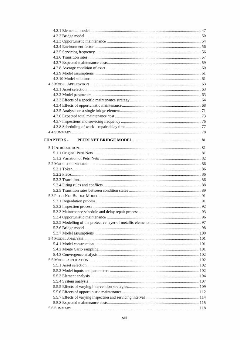
4.2.1 Elemental model ............................................................................................................. 47 4.2.2 Bridge model ................................................................................................................... 50 4.2.3 Opportunistic maintenance ............................................................................................. 54 4.2.4 Environment factor ......................................................................................................... 56 4.2.5 Servicing frequency ........................................................................................................ 56 4.2.6 Transition rates................................................................................................................ 57 4.2.7 Expected maintenance costs ............................................................................................ 59 4.2.8 Average condition of asset .............................................................................................. 60 4.2.9 Model assumptions ......................................................................................................... 61 4.2.10 Model solutions ............................................................................................................. 61
4.3 MODEL APPLICATION .............................................................................................................. 63 4.3.1 Asset selection ................................................................................................................ 63 4.3.2 Model parameters ............................................................................................................ 63 4.3.3 Effects of a specific maintenance strategy ...................................................................... 64 4.3.4 Effects of opportunistic maintenance .............................................................................. 68 4.3.5 Analysis on a single bridge element ................................................................................ 71 4.3.6 Expected total maintenance cost ..................................................................................... 73 4.3.7 Inspections and servicing frequency ............................................................................... 76 4.3.8 Scheduling of work – repair delay time .......................................................................... 77
4.4 SUMMARY ............................................................................................................................... 78
CHAPTER 5 - PETRI NET BRIDGE MODEL.................................................................... 81
5.1 INTRODUCTION ........................................................................................................................ 81 5.1.1 Original Petri Nets .......................................................................................................... 81 5.1.2 Variation of Petri Nets .................................................................................................... 82
5.2 MODEL DEFINITIONS ................................................................................................................ 86 5.2.1 Token .............................................................................................................................. 86 5.2.2 Place ................................................................................................................................ 86 5.2.3 Transition ........................................................................................................................ 86 5.2.4 Firing rules and conflicts................................................................................................. 88 5.2.5 Transition rates between condition states ....................................................................... 89
5.3 PETRI-NET BRIDGE MODEL ..................................................................................................... 91 5.3.1 Degradation process ........................................................................................................ 91 5.3.2 Inspection process ........................................................................................................... 92 5.3.3 Maintenance schedule and delay repair process ............................................................. 93 5.3.4 Opportunistic maintenance ............................................................................................. 96 5.3.5 Modelling of the protective layer of metallic elements ................................................... 97 5.3.6 Bridge model ................................................................................................................... 98 5.3.7 Model assumptions ....................................................................................................... 100
5.4 MODEL ANALYSIS .................................................................................................................. 101 5.4.1 Model construction ....................................................................................................... 101 5.4.2 Monte Carlo sampling ................................................................................................... 101 5.4.3 Convergence analysis .................................................................................................... 102
5.5 MODEL APPLICATION ............................................................................................................. 102 5.5.1 Asset selection .............................................................................................................. 102 5.5.2 Model inputs and parameters ........................................................................................ 102 5.5.3 Element analysis ........................................................................................................... 104 5.5.4 System analysis ............................................................................................................. 107 5.5.5 Effects of varying intervention strategies...................................................................... 109 5.5.6 Effects of opportunistic maintenance ............................................................................ 112 5.5.7 Effects of varying inspection and servicing interval ..................................................... 114 5.5.8 Expected maintenance costs .......................................................................................... 115
5.6 SUMMARY ............................................................................................................................. 118

ix
CHAPTER 6 - MARKOV AND PETRI NET MODEL COMPARISON......................... 119
6.1 INTRODUCTION ...................................................................................................................... 119 6.2 PREDICTING COMPONENT FUTURE AVERAGE CONDITION ....................................................... 119 6.3 PREDICTING COMPONENT FUTURE CONDITION PROFILE ......................................................... 123 6.4 PREDICTING ASSET FUTURE AVERAGE CONDITION ................................................................. 126 6.5 PREDICTING MAINTENANCE COST .......................................................................................... 128 6.6 MODEL PERFORMANCES ........................................................................................................ 130 6.7 SUMMARY ............................................................................................................................. 131
CHAPTER 7 - BRIDGE MAINTENANCE OPTIMISATION ......................................... 133
7.1 INTRODUCTION ...................................................................................................................... 133 7.1.1 Genetic Algorithm optimisation .................................................................................... 134 7.1.2 Multi-objectives GA (MOGA) optimisation ................................................................. 135 7.1.3 Optimisation procedure ................................................................................................. 136
7.2 MARKOV BRIDGE MODEL OPTIMISATION ............................................................................... 137 7.2.1 Objective functions ....................................................................................................... 137 7.2.2 Variables ....................................................................................................................... 138 7.2.3 Variable encoding and decoding ................................................................................... 140 7.2.4 The population .............................................................................................................. 142 7.2.5 Fitness function ............................................................................................................. 142 7.2.6 Paring (selection function) ............................................................................................ 144 7.2.7 Mating ........................................................................................................................... 145 7.2.8 Mutation ........................................................................................................................ 146 7.2.9 Next generation and convergence ................................................................................. 146
7.3 RESULTS AND DISCUSSIONS ................................................................................................... 147 7.3.1 Optimum policies .......................................................................................................... 147 7.3.2 Comparison to industry maintenance policy ................................................................. 151
7.4 PETRI-NET BRIDGE MODEL OPTIMISATION ............................................................................. 152 7.4.1 Objective functions ....................................................................................................... 152 7.4.2 Variables ....................................................................................................................... 153 7.4.3 Hybrid optimisation ...................................................................................................... 153
7.5 RESULTS AND DISCUSSIONS ................................................................................................... 156 7.5.1 Optimum policies .......................................................................................................... 156 7.5.2 Optimisation performance............................................................................................. 159
7.6 SUMMARY ............................................................................................................................. 161
CHAPTER 8 - CONCLUSIONS .......................................................................................... 162
8.1 SUMMARY AND CONCLUSIONS ............................................................................................... 162 8.2 RESEARCH CONTRIBUTIONS ................................................................................................... 165 8.3 FUTURE WORKS ..................................................................................................................... 167
REFERENCES .............................................................................................................................. 168
APPENDIX A DATA ANALYSIS AND DEGRADATION STUDY ................................ 174
A-1 DATA PREPARATION ...................................................................................................... 174 i. Data cleansing ..................................................................................................................... 174 ii. Data combining .................................................................................................................. 175 iii. Data filtering ..................................................................................................................... 177
A-2 TYPICAL METAL UNDERBRIDGE ELEMENTS ................................................................... 178 A-3 ELEMENT CONDITION STATES ........................................................................................ 179 A-4 COMPONENT DEGRADATION ANALYSIS ......................................................................... 184
i. Metal Main Girder .............................................................................................................. 184 ii. Bridge Deck ....................................................................................................................... 188

x
iii. Metal Deck ....................................................................................................................... 189 iv. Concrete Deck .................................................................................................................. 192 v. Timber Deck ...................................................................................................................... 194 vi. Bearing .............................................................................................................................. 197 vii. Abutment ......................................................................................................................... 199
APPENDIX B ENVIRONMENT ADJUSTMENT FACTOR ............................................... 200
APPENDIX C MARKOV BRIDGE MODEL .................................................................... 201
C-1 TRANSITION RATE MATRIX ............................................................................................ 201 C-2 EXPECTED WLCCS ....................................................................................................... 203
APPENDIX D PETRI-NET BRIDGE MODEL ................................................................. 204
D-1 DEGRADATION OF PROTECTIVE COATING AND ITS EFFECTS ON METAL ELEMENT .......... 204 D-2 MODEL RESULTS - ELEMENT ANALYSIS FOR ALL BRIDGE COMPONENTS ........................ 205 D-3 MODEL RESULTS – SYSTEM ANALYSIS FOR VARYING MAINTENANCE POLICIES ............. 214

1
Chapter 1 - Introduction
1.1 Background and research motivation
The function of a railway bridge is to provide a stable support to
the track at an appropriate gradient and alignment along the line.
Railway bridges carry the track through, over or under obstacles
along the routes. Network Rail owns and maintains most of the
railway bridges in the UK railway network. Bridges are classified
into two main types (Network Rail, 2007b):
Under-bridges: carry rail traffic across a geographic feature
or obstruction such as a road, river, valley, estuary, railway
etc.
Over-bridges: carry another service (roadway, footway,
bridleway, public utility, etc.) over the railway. This asset
group includes public highways as well as accommodation
and occupation bridges.
Each type of the bridge is further categorised by the main
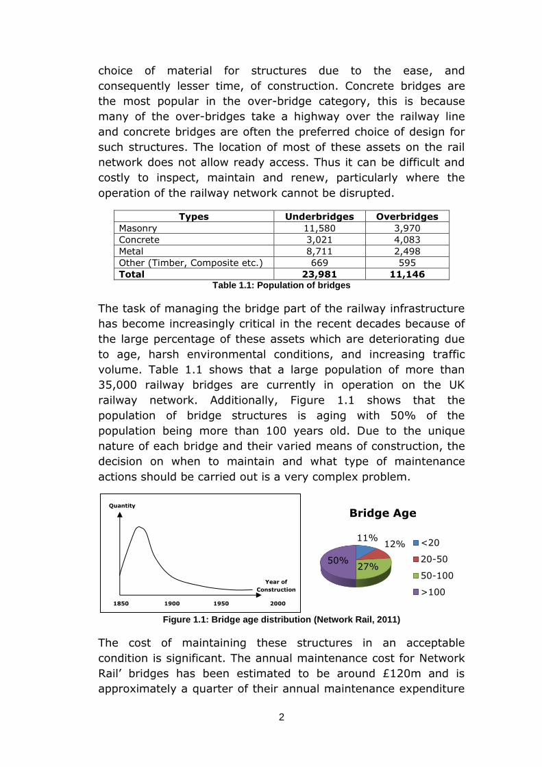
material used in their construction. Table 1.1 shows the
population of all bridges under Network Rail management. Initial
observation of the population is that, there is a large number of
masonry bridges in the UK, almost half of the under-bridge
population and a third of the over-bridge population are masonry.
This is because the British railway is the oldest railway system in
the world, civil structures were primarily built using bricks and
masonry and the majority of the structures built many years ago,
which have been strengthened and upgraded, are still in
operation. Metal bridges are the second most frequent in the
population as a result of a period where iron was the preferred
2
choice of material for structures due to the ease, and
consequently lesser time, of construction. Concrete bridges are
the most popular in the over-bridge category, this is because
many of the over-bridges take a highway over the railway line
and concrete bridges are often the preferred choice of design for
such structures. The location of most of these assets on the rail
network does not allow ready access. Thus it can be difficult and
costly to inspect, maintain and renew, particularly where the
operation of the railway network cannot be disrupted.
Types Underbridges Overbridges
Masonry 11,580 3,970
Concrete 3,021 4,083
Metal 8,711 2,498
Other (Timber, Composite etc.) 669 595
Total 23,981 11,146 Table 1.1: Population of bridges
The task of managing the bridge part of the railway infrastructure
has become increasingly critical in the recent decades because of
the large percentage of these assets which are deteriorating due
to age, harsh environmental conditions, and increasing traffic
volume. Table 1.1 shows that a large population of more than
35,000 railway bridges are currently in operation on the UK
railway network. Additionally, Figure 1.1 shows that the
population of bridge structures is aging with 50% of the
population being more than 100 years old. Due to the unique
nature of each bridge and their varied means of construction, the
decision on when to maintain and what type of maintenance
actions should be carried out is a very complex problem.
Figure 1.1: Bridge age distribution (Network Rail, 2011)
The cost of maintaining these structures in an acceptable
condition is significant. The annual maintenance cost for Network
Rail’ bridges has been estimated to be around £120m and is
approximately a quarter of their annual maintenance expenditure
11% 12%
27% 50%
Bridge Age
<20
20-50
50-100
>1001850 1900 1950 2000
Quantity
Year of
Construction

3
for civil structures (Network Rail, 2013). The cost of maintenance
has to be agreed with the Office of Rail Regulator (ORR) over five-
year control periods (CP). Network Rail is required to estimate the
expected maintenance, renewal and improvement costs and
provide a strong justification for those figures before submission
to the ORR. In the submissions for the previous control period
(CP4, from 2009/10 to 20013/14), Network Rail utilised the Civil
Engineering Cost and Strategy Evaluation (CECASE) tool which
was developed for this purpose. The tool calculates the whole life
cost, for a single asset type, for a range of possible renewal,
maintenance and utilisation options. However, following critical
review by the ORR, a more robust and flexible tool is required.
There is therefore a desire is to formulate a bridge model and a
decision making process which will enable a strategy to be
established which will enable assets to be maintained and
renewed to minimise the whole life costs. The quality of the
decisions made with such an approach is dependent upon how
well the deterioration processes of the assets over time are
understood. Historical data can be used to study the degradation
process of bridge elements. Models can be formulated to predict
the future condition of bridge asset along with the effect that
interventions such as servicing, repair, and element replacement
will produce. Intervention costs can then be integrated into the
model and an optimisation can be performed to determine the
optimum maintenance strategy indicating what actions need to be
taken at what time and where in order to minimise the whole life
spend whilst providing an acceptable service and safety
performance.
1.2 Research aims and objectives
1.2.1 Aims
The goal of the research presented in this thesis is to develop
complete bridge asset models. The focus is on accurate prediction
of the future asset condition at both the whole asset and
component levels. Maintenance is then incorporated into the
model to demonstrate the effect of different intervention
strategies. An optimisation is then performed to support the
decision making process to establish the optimum maintenance
policy.
The principle goals of the research are:

4
Examine the historical data records for the maintenance
actions that have been carried out on Network Rail bridges
of similar material and construction.
Establish a bridge model to estimate how much assets
deteriorate over time.
Estimate the future work volume for the whole asset at
elemental level.
Predict an optimal strategy for maintenance (servicing,
repair, replacement) in order to minimise the whole life
costs.
1.2.2 Objectives
The principle objectives of this research project are:
Develop a novel deterioration model that does not use the
current condition rating system, the model would use
information provided from the historical maintenance
records to understand what interventions have been carried
out at different stages of an asset’s life.
Develop a bridge model based on the widely accepted
Markov modelling approach. The model will take into
account different factors that affect the deterioration and
maintenance planning process. Thus the model is
considered in much more detail than other bridge models
available in the literature.
Develop a bridge model based on an approach which is
novel for bridge condition prediction – the Petri-Net
modelling approach. The improvements and advantages
along with the disadvantages of the method over the
traditional modelling approach will be identified and
discussed.
Optimise the bridge maintenance strategy to minimise the
whole life costs whilst providing an acceptable condition
state using the Genetic Algorithm technique.
1.3 Thesis outline
The thesis is organized as follows:
Chapter 2 provides a detailed review of the literature reporting
the previous research conducted on modelling the degradation
process of bridges and bridge elements. Different modelling
approaches are reviewed and their advantages and disadvantages
are critically appraised.
5
Chapter 3 presents a novel method of modelling the asset
deterioration process, this involves constructing a timeline of all
historical work done of a bridge element and analysing the time of
the component reaching different intervention actions in order to
establish a component lifetime distribution. The analysis
methodology is presented in detail following a discussion of the
available datasets. The results obtained from the analysis are also
presented.
Chapter 4 demonstrates a Markov modelling approach to predict
the condition of individual bridge elements along with the effects
that interventions will produce. The development of the bridge
model is also discussed and simulation results are presented to
demonstrate the capability of the model as well as the type of
information the model generates that can be used to support the
asset management strategy selection.
Chapter 5 describes the development of a bridge model using
the Petri-Net (PN) modelling technique. This chapter gives an
overview of the PN method before developing a PN bridge model.
It also discusses, in detail, the modifications to the original PN
modelling technique to suit the problem of modelling bridge asset
condition. The model is then applied to a selected example asset
and simulation results are presented and discussed.
Chapter 6 compares the two bridge models developed in term of
model results and performance.
Chapter 7 presents an optimisation framework based on the
Genetic Algorithm technique as a decision making approach to
select the best maintenance strategy. A high performance hybrid-
optimisation was applied using both the Markov and the Petri-Net
bridge models. The optimisation is a multi-objective optimisation
that looks for the maintenance policies that will produce the
lowest expected maintenance cost whilst maximising the average
condition of the asset.
Chapter 8 summarises the research work, highlights its
contributions, and gives recommendations for future research.

6
7
Chapter 2 - Literature Review
2.1 Introduction
Over the last few decades, numerous papers have appeared in
the literature, which deal with the modelling of bridge asset
management. These studies focused on developing deterioration
models that predict the degradation rates and the future states of
a bridge. These models, reported in this section, use a variety of
techniques. The simplest form of bridge deterioration modelling is
the deterministic model. Deterministic models predict the future
asset conditions deterministically by fitting a straight-line or a
curve (Jiang and Sinha, 1989, Sanders and Zhang, 1994) to
establish a relationship between the bridge condition and age.
Due to the nature of deterministic models that they do not
capture the uncertainty in the data, many studies develop
stochastic models which are considered to provide improved
prediction accuracy (Bu et al., 2013). In stochastic models, the
deterioration process is described by one or more random
variables, therefore this method takes into account the
randomness and uncertainties that arise in the processes that are
being analysed. Amongst the deterministic models, regression
analysis is a methodology widely used, whereas, the Markov-
based model is considered as one of the most common stochastic
techniques adopted. This section focuses on all the studies using
the stochastic approach, starting with the fundamentals of Markov
models before exploring Markov-based and other probabilistic
bridge models available in the literature.
It is important to note that even though some of the reported
models were applied to railway bridges, some were used to
8
predict the deterioration rate and future state of highway bridges.
From the asset management point of view, the two situations
differ from each other since they could be managed by different
authorities e.g. Network Rail and Highway Agency in the UK.
However, in terms of methods and techniques to predict the
future state of a bridge, there are no differences as the
deterioration models for railway bridges can be applied for
highway bridges and vice-versa. This is because the two models
are essentially based on the same mathematical or statistical
techniques. The purpose of this section is to study all the methods
and techniques, reported in the literature to model the
deterioration of bridges. By considering models for highway
bridges and other infrastructure assets, a broader range of
techniques can be studied.
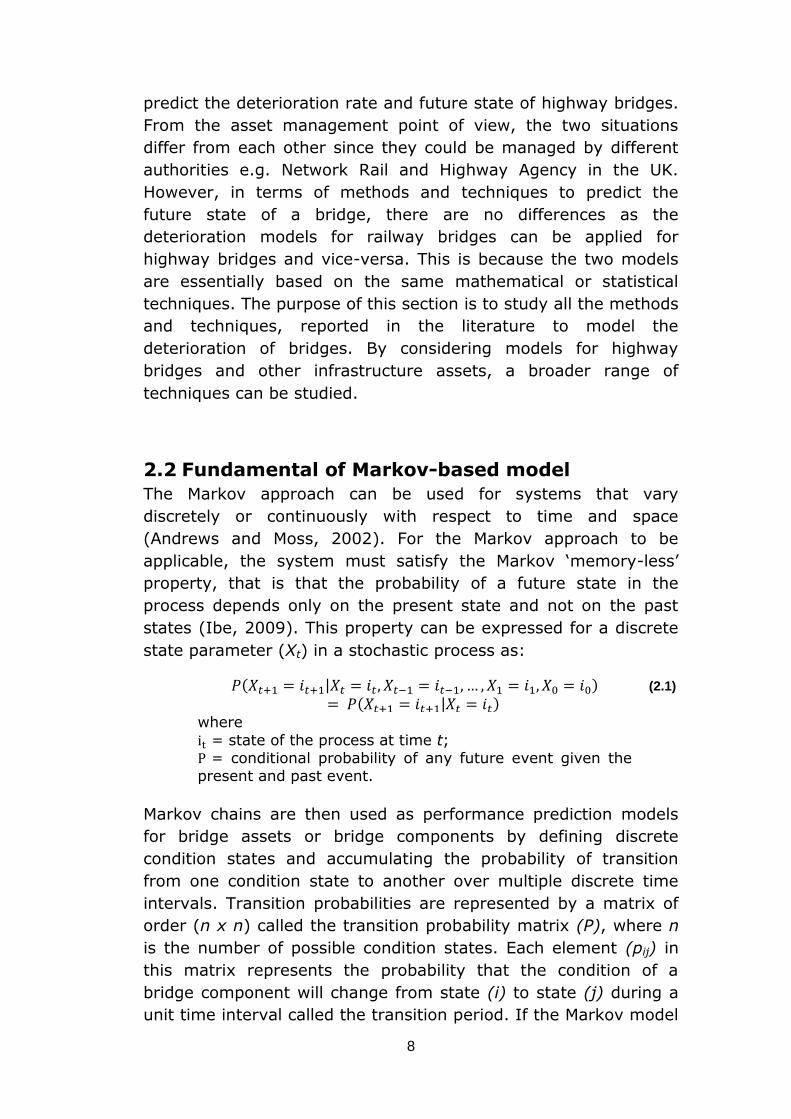
2.2 Fundamental of Markov-based model
The Markov approach can be used for systems that vary
discretely or continuously with respect to time and space
(Andrews and Moss, 2002). For the Markov approach to be
applicable, the system must satisfy the Markov ‘memory-less’
property, that is that the probability of a future state in the
process depends only on the present state and not on the past
states (Ibe, 2009). This property can be expressed for a discrete
state parameter (Xt) in a stochastic process as:
( | ) ( | )
(2.1)
where
= state of the process at time t;
= conditional probability of any future event given the
present and past event.
Markov chains are then used as performance prediction models
for bridge assets or bridge components by defining discrete
condition states and accumulating the probability of transition
from one condition state to another over multiple discrete time
intervals. Transition probabilities are represented by a matrix of
order (n x n) called the transition probability matrix (P), where n
is the number of possible condition states. Each element (pij) in
this matrix represents the probability that the condition of a
bridge component will change from state (i) to state (j) during a
unit time interval called the transition period. If the Markov model
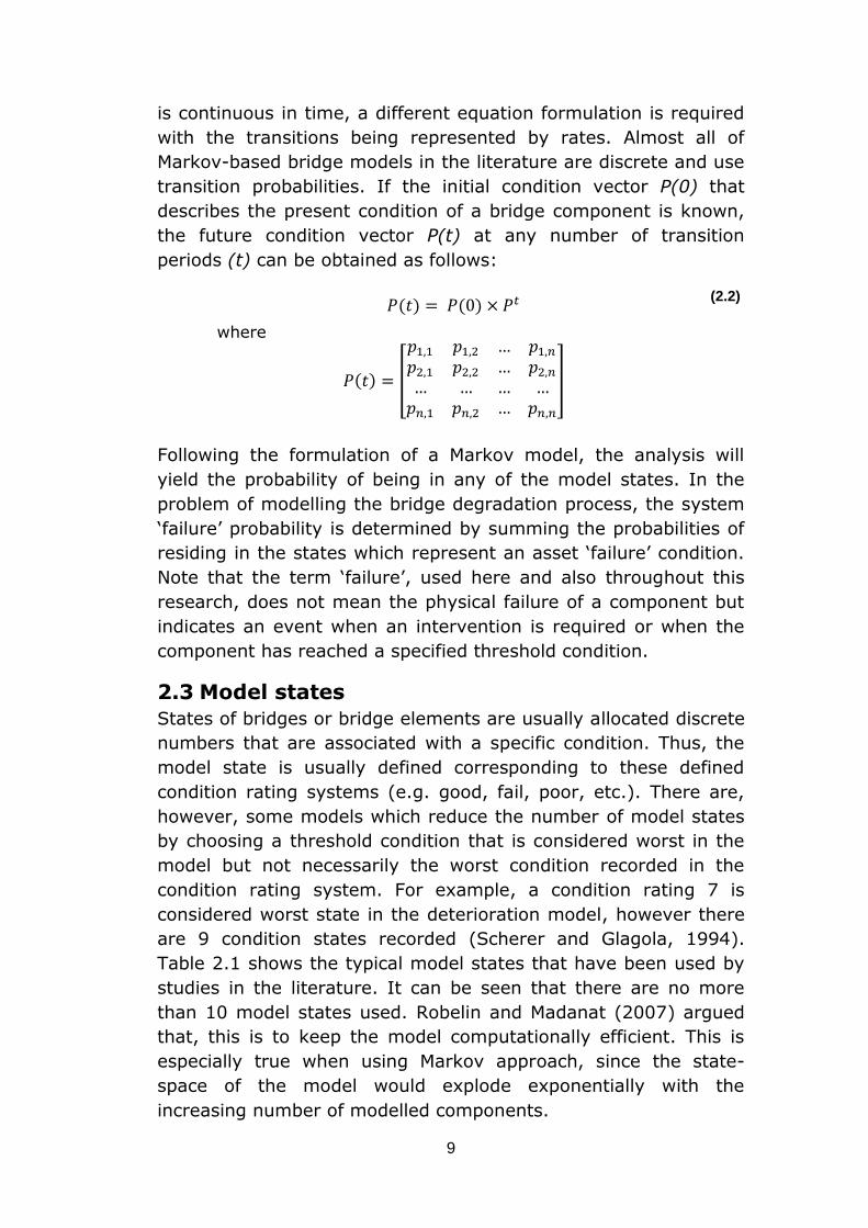
9
is continuous in time, a different equation formulation is required
with the transitions being represented by rates. Almost all of
Markov-based bridge models in the literature are discrete and use
transition probabilities. If the initial condition vector P(0) that
describes the present condition of a bridge component is known,
the future condition vector P(t) at any number of transition
periods (t) can be obtained as follows:
( ) ( ) (2.2)
where
( ) [
]
Following the formulation of a Markov model, the analysis will
yield the probability of being in any of the model states. In the
problem of modelling the bridge degradation process, the system
‘failure’ probability is determined by summing the probabilities of
residing in the states which represent an asset ‘failure’ condition.
Note that the term ‘failure’, used here and also throughout this
research, does not mean the physical failure of a component but
indicates an event when an intervention is required or when the
component has reached a specified threshold condition.
2.3 Model states
States of bridges or bridge elements are usually allocated discrete
numbers that are associated with a specific condition. Thus, the
model state is usually defined corresponding to these defined
condition rating systems (e.g. good, fail, poor, etc.). There are,
however, some models which reduce the number of model states
by choosing a threshold condition that is considered worst in the
model but not necessarily the worst condition recorded in the
condition rating system. For example, a condition rating 7 is
considered worst state in the deterioration model, however there
are 9 condition states recorded (Scherer and Glagola, 1994).
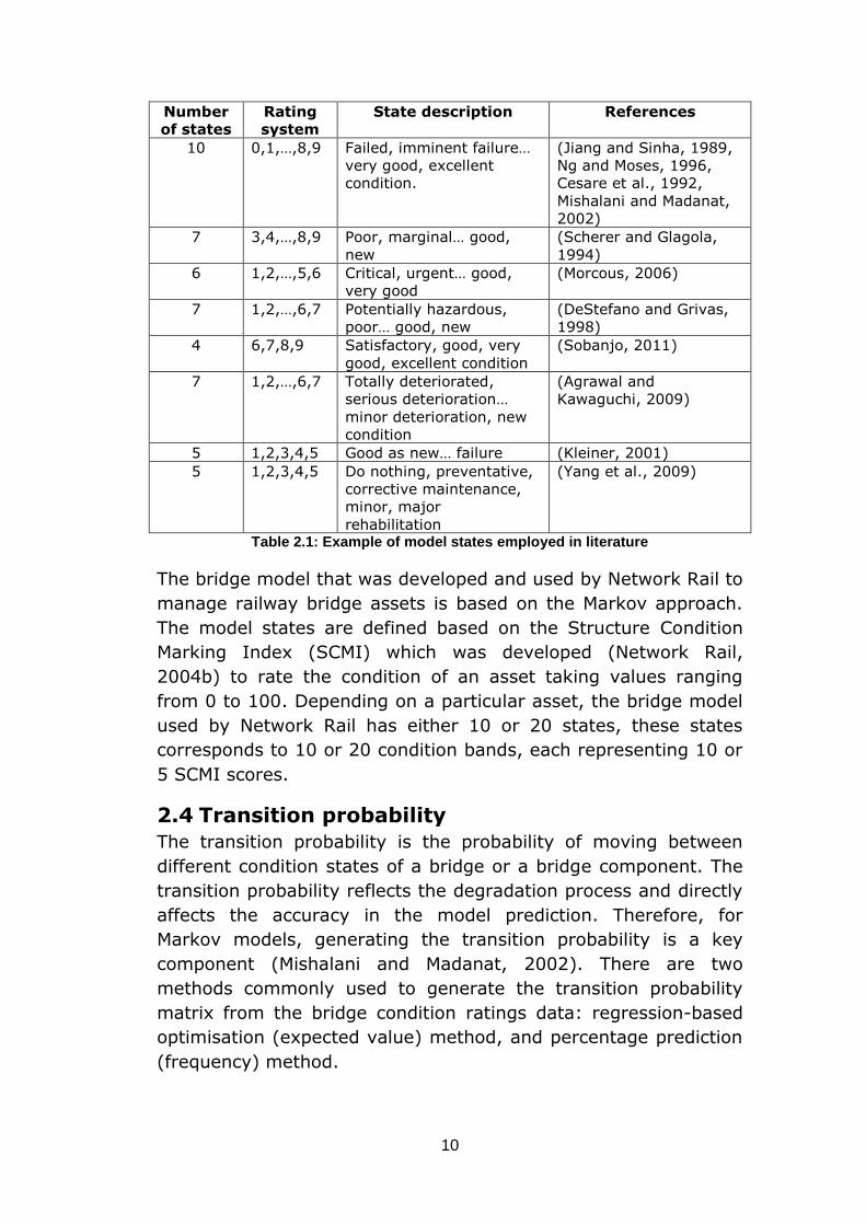
Table 2.1 shows the typical model states that have been used by
studies in the literature. It can be seen that there are no more
than 10 model states used. Robelin and Madanat (2007) argued
that, this is to keep the model computationally efficient. This is
especially true when using Markov approach, since the state-
space of the model would explode exponentially with the
increasing number of modelled components.
10
Number
of states
Rating
system
State description References
10 0,1,…,8,9 Failed, imminent failure…
very good, excellent
condition.
(Jiang and Sinha, 1989,
Ng and Moses, 1996,
Cesare et al., 1992,
Mishalani and Madanat,
2002)
7 3,4,…,8,9 Poor, marginal… good,
new
(Scherer and Glagola,
1994)
6 1,2,…,5,6 Critical, urgent… good,
very good
(Morcous, 2006)
7 1,2,…,6,7 Potentially hazardous,
poor… good, new
(DeStefano and Grivas,
1998)
4 6,7,8,9 Satisfactory, good, very
good, excellent condition
(Sobanjo, 2011)
7 1,2,…,6,7 Totally deteriorated,
serious deterioration…
minor deterioration, new
condition
(Agrawal and
Kawaguchi, 2009)
5 1,2,3,4,5 Good as new… failure (Kleiner, 2001)
5 1,2,3,4,5 Do nothing, preventative,
corrective maintenance,
minor, major
rehabilitation
(Yang et al., 2009)
Table 2.1: Example of model states employed in literature
The bridge model that was developed and used by Network Rail to
manage railway bridge assets is based on the Markov approach.
The model states are defined based on the Structure Condition
Marking Index (SCMI) which was developed (Network Rail,
2004b) to rate the condition of an asset taking values ranging
from 0 to 100. Depending on a particular asset, the bridge model
used by Network Rail has either 10 or 20 states, these states
corresponds to 10 or 20 condition bands, each representing 10 or
5 SCMI scores.
2.4 Transition probability
The transition probability is the probability of moving between
different condition states of a bridge or a bridge component. The
transition probability reflects the degradation process and directly
affects the accuracy in the model prediction. Therefore, for
Markov models, generating the transition probability is a key
component (Mishalani and Madanat, 2002). There are two
methods commonly used to generate the transition probability
matrix from the bridge condition ratings data: regression-based
optimisation (expected value) method, and percentage prediction
(frequency) method.
11
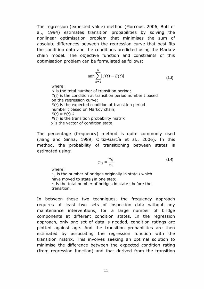
The regression (expected value) method (Morcous, 2006, Butt et
al., 1994) estimates transition probabilities by solving the
nonlinear optimisation problem that minimises the sum of
absolute differences between the regression curve that best fits
the condition data and the conditions predicted using the Markov
chain model. The objective function and constraints of this
optimisation problem can be formulated as follows:
∑| ( ) ( )|
(2.3)
where:
is the total number of transition period;
( ) is the condition at transition period number t based
on the regression curve; ( ) is the expected condition at transition period
number t based on Markov chain; ( ) ( )
( ) is the transition probability matrix
is the vector of condition state
The percentage (frequency) method is quite commonly used
(Jiang and Sinha, 1989, Ortiz-García et al., 2006). In this
method, the probability of transitioning between states is
estimated using:
(2.4)
where:
is the number of bridges originally in state which
have moved to state in one step;
is the total number of bridges in state before the transition.
In between these two techniques, the frequency approach
requires at least two sets of inspection data without any
maintenance interventions, for a large number of bridge
components at different condition states. In the regression
approach, only one set of data is needed, condition ratings are
plotted against age. And the transition probabilities are then
estimated by associating the regression function with the
transition matrix. This involves seeking an optimal solution to
minimise the difference between the expected condition rating
(from regression function) and that derived from the transition
12
matrix. Therefore the frequency approach was usually used when
the data is available.
It is realised that the bridge condition databases used in all the
studied in the literature do not accommodate these methods.
These databases would normally, at best, contain records that
only go back as far as the last two decades, the condition ratings
usually do not change significantly during short-term periods.
Moreover, the database would usually be filtered to remove data
indicating a rise in condition rating (due to the effect of
improvement or maintenance), this further reduces the available
data for the analysis. All these factors exhibit the inaccuracy in
the determination of the transition probability which directly
affects the prediction of future asset condition.
2.5 Markov model
The Markov approach is the most common stochastic techniques
that has been used over 20 years in modelling the deterioration of
bridges and bridge elements.
Jiang and Sinha (1989) were one of the first to demonstrate the
use of a Markov model in predicting the deterioration rate of
bridges. Their paper focused on discussing the methodology in
estimating the transition probability based on the condition score
data of bridges at different ages. The method used in this paper is
the expected value method. Although the paper has
demonstrated the method, there was no real application on actual
bridge condition data.
Cesare et al. (1991) describe methods for utilising Markov chains
in the evaluation of highway bridge deterioration. A study was
carried out based on the empirical data of 850 bridges in New
York State. The data contains bridge element condition ratings on
the scale of 1 to 7 with 7 being new and 1 being the worst
condition. Assuming the deterioration of each element is
independent of all other bridge elements, the Markov model was
then applied to predict the evolution of the average condition
rating of a set of bridges and the expected value of condition
rating for a single bridge. The paper discussed that, the effects of
the lack of supporting data would require the results produced in
this paper to be further validated and suggested that the Markov
model employed would need more data in order to produce
accurate results.
13
Scherer and Glagola (1994) explored the applicability of the
Markov approach on the modelling of the bridge deterioration
process. The authors developed a Markov bridge model for a
single bridge asset with the intention of using a single model to
manage the entire population of 13,000 bridges in the state of
Virginia, USA. An individual bridge is considered to have 7 states.
It was pointed out that the Markov model size would be
computationally intractable even for a population of 10 bridges
since the model size would be 710 (approximately 300,000,000
states). To tackle this problem, the author developed a
classification system which group bridges according to: route type
(interstate, primary, secondary); climate; traffic loading; bridge
type (concrete, timber deck); bridge spans (single, multiple);
bridge age (0-20, 21-40, 41 years and older). A 7-state Markov
model was then developed that was representative of a bridge in
each bridge class. In summary, the paper addressed the issues in
state-space combinatorial explosion associated with Markov
models, and verified that the Markov assumption is acceptable in
bridge asset management modelling.
Morcous (2006) also adopted Markov chain models for predicting
the future condition of bridge components. A study was carried
out to predict the condition of a bridge deck using the data from
9,678 structures of 57 different types of highway structure in
Quebec, Canada. The data includes 500,924 inspection records
from 1997 to 2000 that recorded the structure condition index
from 0 to 100 with the greater the condition the better. The paper
highlighted several assumptions used in the model such as:
bridge inspections are performed at pre-determined fixed time
intervals (constant inspection period); future bridge condition
depends only on present condition and not the past condition. The
transition probabilities were determined using the frequency
method. Data with increased condition ratings were removed to
eliminate the effects of maintenance on the data. The paper
investigated that the inspection period which was not constant,
and follows a normal distribution. The effects were found by
adjusting the developed transition probabilities for the variation in
the inspection periods and the predicted performance before and
after adjustments. The adjusted rates used Bayes’ rules, and the
paper shows that the variation in the inspection period may result
in a 22% error in predicting the life of component.
14
All of the Markov models presented are simple, they predict the
future condition for a single bridge component or a whole bridge.
Complete bridge asset model, that describes a complete bridge
structure including bridge elements, was not developed. In
additional, Markov-based model cannot efficiently consider the
interactive effects of the deterioration rates between different
bridge elements (Sianipar and Adams, 1997).
2.6 Reliability–based model
The degradation process of a bridge element can be modelled
using the ‘life data’ analysis technique. This technique is popular
in system reliability studies. DeStefano and Grivas (1998)
demonstrated that the ‘life data’ analysis method can be applied
for the development of probabilistic bridge deterioration models
on the basis of the available information. The data required using
this technique is the times to a specified transition event. This
event is found by looking at the change in the condition rating,
i.e. a drop in condition score, for a bridge element recorded in the
database. This technique considers both complete and censored
lifetime data. Complete data indicates the transition time
associated with state transition events that have been observed.
Censored data indicates the state transition event that has not
been observed within the analysis period, this might be because
the component was replaced while in its initial condition state or
the analysis period is not long enough for the transition to occur.
In DeStefano and Grivas (1998) paper, the Kaplan and Meier
method is applied to these data to calculate non-parametric
estimates of cumulative transition probability corresponding to
transition times and specific transition events. The degradation
process is described by the transition probability which is defined
as this cumulative probability. A study was carried out using the
inspection data of 123 bridges in New York, USA. The paper
suggested that the reliability-based method recognises the
‘censored’ nature of bridge inspection data and incorporates these
data into the deterioration modelling process. The paper also
pointed out the subjective nature of inspection data and the
inherent error this adds to the model. The paper demonstrated
the approach by analysing the bridge component lifetime data,
although it is suggested that better fitting and more robust
distributions could be used to fit to the data.
15
Frangopol et al. (2001) used a reliability index (β) that measures
the bridge safety instead of condition. The reliability index was
previously developed by Thoft-Christensen (1999) and is defined
in Table 2.2. The deterioration rate of a bridge is now the
deterioration rate of the reliability index.
State State no β
Extremely good 5 >10
Very good 4 [8,10]
Good 3 [6,8]
Acceptable 2 [4.6,6]
Non-acceptable 1 <4.6 Table 2.2: Definition of the bridge reliability index (Thoft-Christensen, 1999)
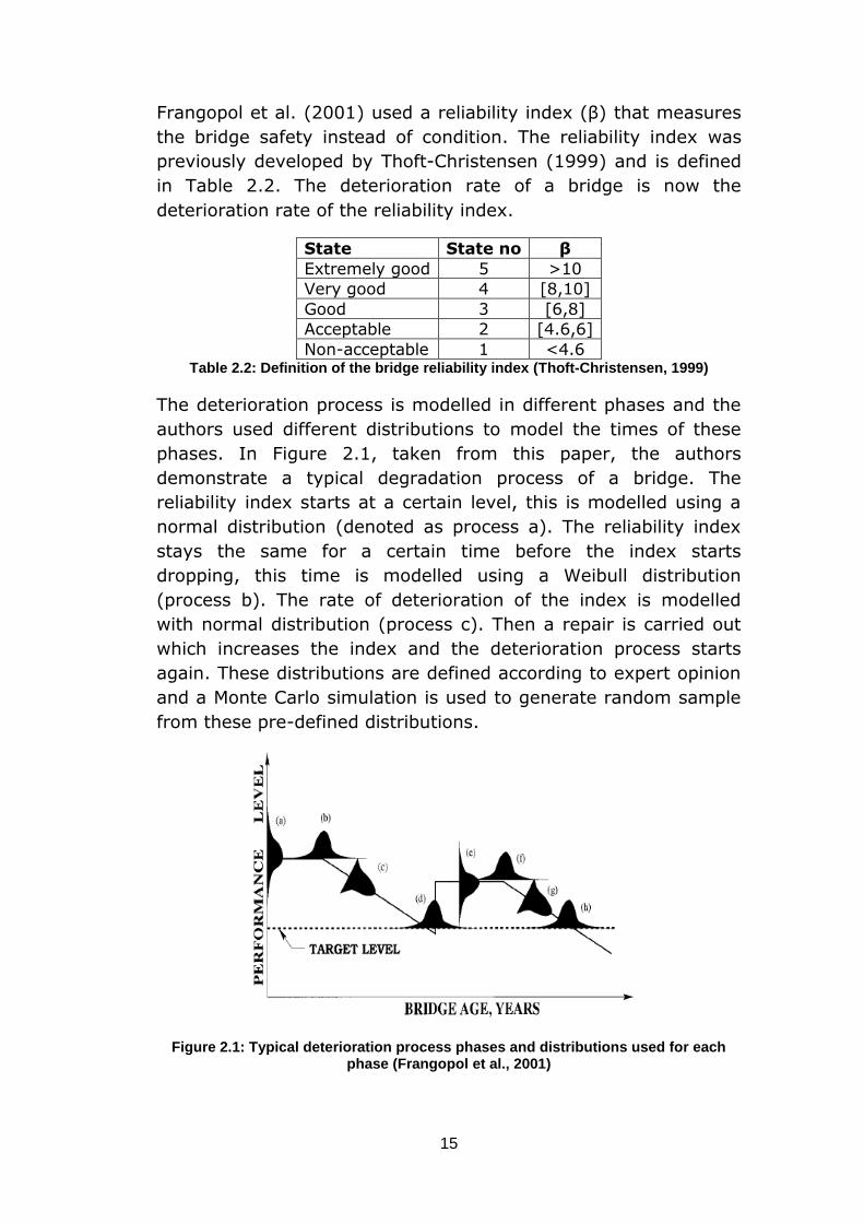
The deterioration process is modelled in different phases and the
authors used different distributions to model the times of these
phases. In Figure 2.1, taken from this paper, the authors
demonstrate a typical degradation process of a bridge. The
reliability index starts at a certain level, this is modelled using a
normal distribution (denoted as process a). The reliability index
stays the same for a certain time before the index starts
dropping, this time is modelled using a Weibull distribution
(process b). The rate of deterioration of the index is modelled
with normal distribution (process c). Then a repair is carried out
which increases the index and the deterioration process starts
again. These distributions are defined according to expert opinion
and a Monte Carlo simulation is used to generate random sample
from these pre-defined distributions.
Figure 2.1: Typical deterioration process phases and distributions used for each phase (Frangopol et al., 2001)
16
The authors have developed a reliability index and believed that it
has the added benefit to measure the deterioration process,
however the benefit cannot be seen. Moreover, the index is an
indicator for a bridge or a group of bridges and thus will have no
indication of the condition of the bridge elements. The distribution
parameters used in the paper are defined based on expert
judgement, this leads to inaccuracy in the degradation model. It
is realised that, with the flexibility of the demonstrated approach,
there are many scenarios which can be modelled. However, a
different degradation model would be required for each scenario.
The model also would require a large computation time.
Noortwijk and Klatter (2004) performed a statistical analysis on
the life time of a bridge by fitting Weibull distribution to the
lifetimes of demolished bridges (complete lifetime) and current
ages of existing bridges (censored/incomplete lifetime). A
distribution of the times between when the bridge was built and
when the bridge is renewed was obtained from this study. There
are, however, several issues with the study. Firstly, the data type
does not reflect the demolishing and replacement of bridges due
to deterioration failure but due to the change in requirement.
Secondly, only one ‘failure’ mode is considered which is the
complete failure of the bridge.
Sobanjo et al. (2010) presented a study in understanding the
natural deterioration process (without significant improvement) of
bridges in Florida, USA. The authors studied the failure times
(time to reach a specified condition threshold) and sojourn times
(time of staying in one condition state) at various condition
states. The time (age) of the bridge at transition was assumed to
be the average of two estimates: the age at departure and age at
arrival at a given condition state. Weibull distribution was
reported as a best fit to model the uncertainties in the failure
times obtained. The study was on bridge decks and
superstructures using the NBI (National Bridge Inspection)
database with the bridge condition reports from 1992 to 2005.
Note that this database is used in the USA and there are 9
condition ratings for a bridge component. The assumption used in
this paper is that no major improvement is done to the bridge,
thus data which indicates improvement, i.e. increase ratings
between consequent inspections, are subsequently removed. The
Weibull shape parameters reported from this study are generally
17
quite high (larger than 2), this means that the results produced
by the paper should be further verified. Despite few limitations,
the paper demonstrated that, with the shape parameters larger
than 1, the deterioration rate of bridge element is increasing over
time.
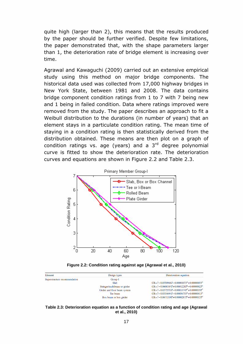
Agrawal and Kawaguchi (2009) carried out an extensive empirical
study using this method on major bridge components. The
historical data used was collected from 17,000 highway bridges in
New York State, between 1981 and 2008. The data contains
bridge component condition ratings from 1 to 7 with 7 being new
and 1 being in failed condition. Data where ratings improved were
removed from the study. The paper describes an approach to fit a
Weibull distribution to the durations (in number of years) that an
element stays in a particulate condition rating. The mean time of
staying in a condition rating is then statistically derived from the
distribution obtained. These means are then plot on a graph of
condition ratings vs. age (years) and a 3rd degree polynomial
curve is fitted to show the deterioration rate. The deterioration
curves and equations are shown in Figure 2.2 and Table 2.3.
Figure 2.2: Condition rating against age (Agrawal et al., 2010)
Table 2.3: Deterioration equation as a function of condition rating and age (Agrawal et al., 2010)
18
In a later study (Agrawal et al., 2010), the authors compared the
deterioration curves produced by this method and those produced
by applying the Markov approach. The comparisons were on the
bridge primary members such as: girder, deck, pier cap,
abutment or pier bearing, abutment. The paper reports that the
deterioration rates produced by the Weibull approach are
generally higher than those resulting from the Markov approach.
The values of shape parameter were greater than one which
clearly shows the bridge component deterioration rate is
durational dependent and the consideration of censored data
illustrated that the Weibull approach provides a better fit to the
observed bridge element conditions. The authors have
demonstrated the reliability approach on the modelling of the
bridge component degradation process. The mean time to
different condition states is obtained from the fitted Weibull
distribution. However the fitting of a polynomial curve to these
means to describe the degradation process eradicates the
advantage that the reliability-based method presents. This is
because the mean time will not fully explain the degradation
process described by a Weibull distribution.
It was found that, for all the studies which employed the
reliability-based approach, the data used in these studies are the
condition ratings. The data required for the analysis is the time to
an event where the element condition changes, it was then
assumed that the transition events occur at the midpoint between
inspection dates. This reason is that the actual date when a
transition event happens is not observed. This assumption is
invalid when the inspection intervals are wide relatively to the
assumed distribution width. This introduces bias in the duration
times that lead to errors in the accuracy of the modelled
degradation process.
2.7 Semi–Markov model
The Markov model is based on the assumption of exponential
distribution for duration for the sojourn/holding times at each
specific bridge condition. This property, when used in modelling
bridge deterioration, suggests that the probability for a bridge to
move from its current state to another more deteriorated state is
constant in the discrete period of time considered and does not
depends on how long it has been in the current state. Semi-
Markov models use different distributions (most of the papers
19
discuss in this section used Weibull distribution) to model these
duration times of a bridge staying in a specific condition. The
derivation of the duration times and the fitting of the Weibull
distribution to these times is very similar to the method discussed
previously for reliability-based models.
The semi-Markov process could be conceived as a stochastic
process governed by two different and independent random-
generating mechanisms. Let T1, T2, …, Tn-1 be random variables
denoting the duration times in states 1, 2, …, n-1. Their
corresponding probability density functions (pdfs), cumulative
density functions (cdfs) and survival functions (sfs) are thus
denoted as fi(t), Fi(t), Si(t). Ti→k is a random variable denoting the
sum of the times residing in states i, i+1, …, k-1. Thus, Ti→k is the
time it will take the process to go from state i to state k. In
addition, fi→k(t), Fi→k(t), Si→k(t) are the pdf, cdf and sf of Ti→k,
respectively.
If the asset state is in state 1 at time t, the conditional probability
that it will transit to the next state in the next time step ∆t is
given by:
( | ) ( ) ( )
( ) (2.5)
when t = 0, the process entered into state 1, i.e. new asset. If the time step is assumed to be small enough to
exclude a two-state deterioration, ∆t can be omitted.
If the process is in state 2 at time t, the conditional probability
that it will transit the next state in the next time step ∆t is given
by:
( | ) ( ) ( )
( ) ( ) (2.6)
Note that the pdf ( ) pertains to Ti→k, which is the random variable denoting the sum of duration times in
states 1 and 2. The survival functions ( ) and ( ) express the simultaneous condition that T1→2 < t and T1 < t
The equation above can then be generalised for subsequent
states by:
20
( | ) ( ) ( )
( ) ( )( )
(2.7)
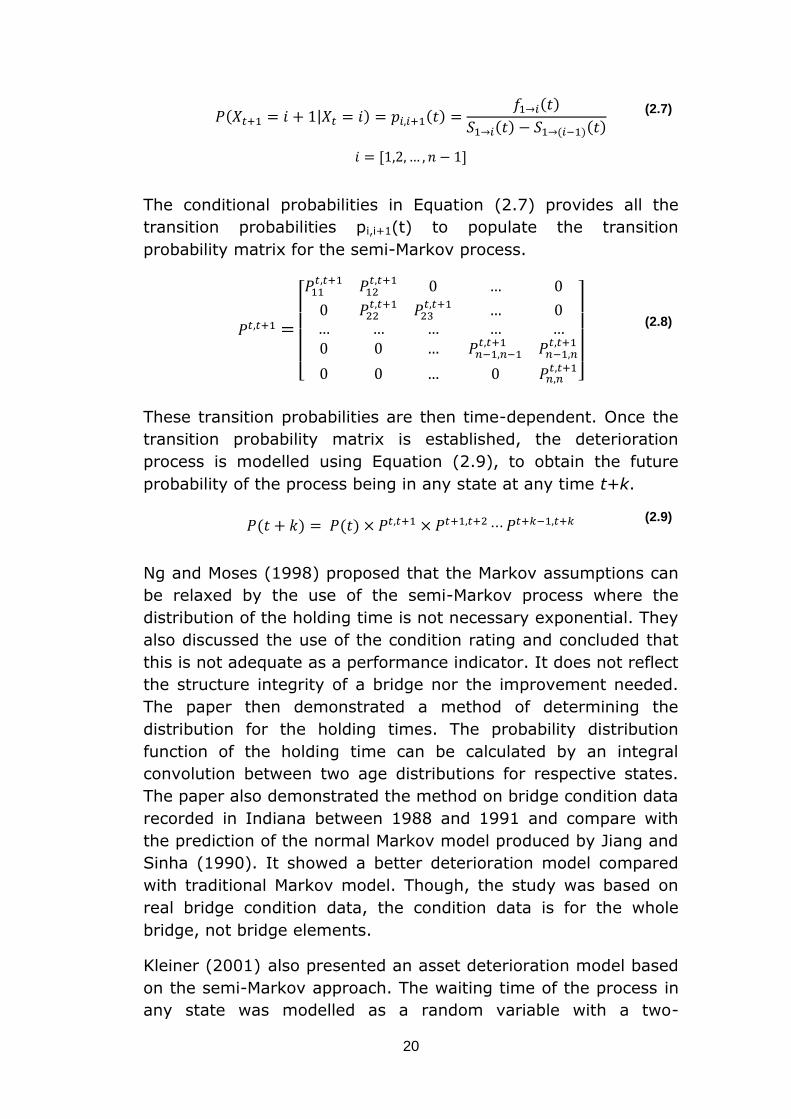
The conditional probabilities in Equation (2.7) provides all the
transition probabilities pi,i+1(t) to populate the transition
probability matrix for the semi-Markov process.
[
]
(2.8)
These transition probabilities are then time-dependent. Once the
transition probability matrix is established, the deterioration
process is modelled using Equation (2.9), to obtain the future
probability of the process being in any state at any time t+k.
( ) ( ) (2.9)
Ng and Moses (1998) proposed that the Markov assumptions can
be relaxed by the use of the semi-Markov process where the
distribution of the holding time is not necessary exponential. They
also discussed the use of the condition rating and concluded that
this is not adequate as a performance indicator. It does not reflect
the structure integrity of a bridge nor the improvement needed.
The paper then demonstrated a method of determining the
distribution for the holding times. The probability distribution
function of the holding time can be calculated by an integral
convolution between two age distributions for respective states.
The paper also demonstrated the method on bridge condition data
recorded in Indiana between 1988 and 1991 and compare with
the prediction of the normal Markov model produced by Jiang and
Sinha (1990). It showed a better deterioration model compared
with traditional Markov model. Though, the study was based on
real bridge condition data, the condition data is for the whole
bridge, not bridge elements.
Kleiner (2001) also presented an asset deterioration model based
on the semi-Markov approach. The waiting time of the process in
any state was modelled as a random variable with a two-
21
parameter Weibull probability distribution. The application of the
model is then demonstrated based on hypothetical data, which
was obtained from expert opinion and perception. Having the
Weibull distribution parameters defined by the experts, the
transition probability matrix was then obtained and the future
condition of the assets was predicted. The paper demonstrated a
model framework based on semi-Markov process, however the
study was based on expert judgement, not the real data.
Mishalani and Madanate (2002) presented a study using the semi-
Markov approach based on empirical data. The data, in this case,
being condition ratings taken from the Indiana Bridge Inventory
(IBI). There are 10 states in the model with 9 being the best and
0 being the worst state. The data set contained 1,460 records
from 1974 to 1984 with two year inspection periods (which means
there are about 5 sets of inspection data per structure). Following
the analysis, data which indicate maintenance were removed. The
following assumptions were also used: the time when at which an
event occurred (condition deterioration) is exactly in the middle of
two recorded inspection i.e. the time when the change in the
condition rating occurs is exactly halfway between the two
inspections; when condition drops by two states, the time in the
intermediate state is assumed to be 1 year. Due to the
unavailability of the data, the prediction study was carried out to
model the degradation process between only three states (state
8, 7, and 6). This means that the empirical study was incomplete
and did not contribute to the model framework established
previously by other authors.
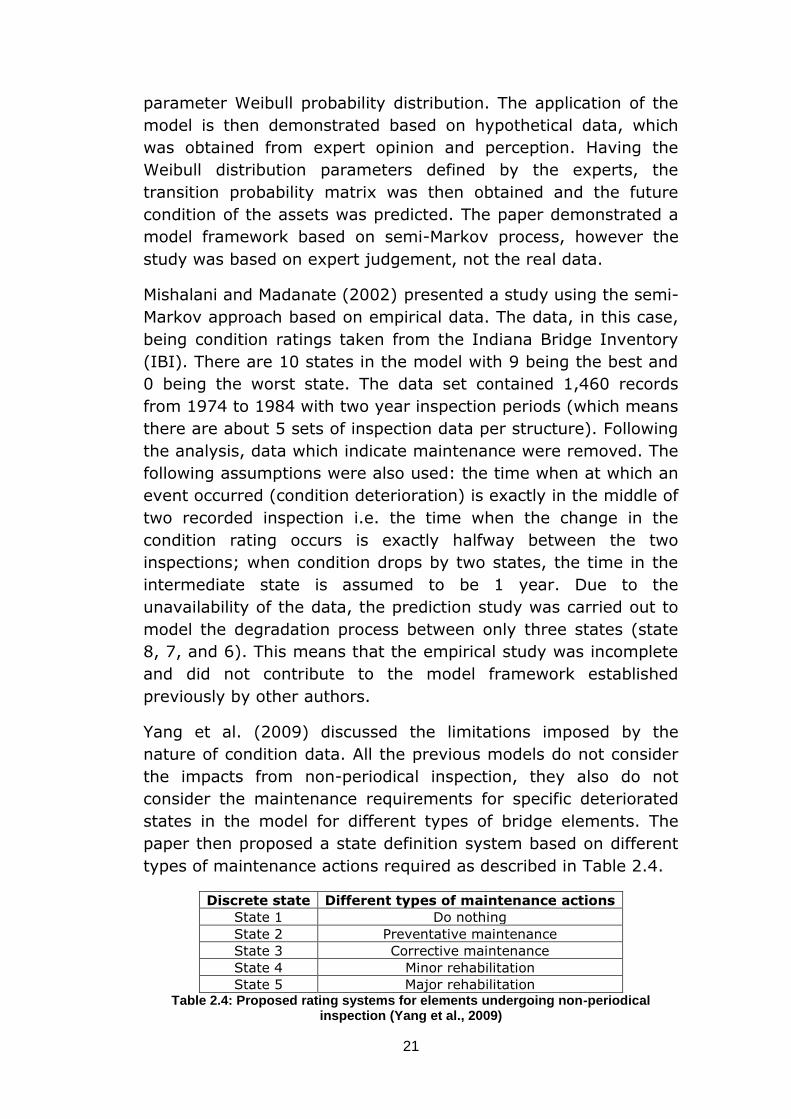
Yang et al. (2009) discussed the limitations imposed by the
nature of condition data. All the previous models do not consider
the impacts from non-periodical inspection, they also do not
consider the maintenance requirements for specific deteriorated
states in the model for different types of bridge elements. The
paper then proposed a state definition system based on different
types of maintenance actions required as described in Table 2.4.
Discrete state Different types of maintenance actions
State 1 Do nothing
State 2 Preventative maintenance
State 3 Corrective maintenance
State 4 Minor rehabilitation
State 5 Major rehabilitation Table 2.4: Proposed rating systems for elements undergoing non-periodical
inspection (Yang et al., 2009)
22
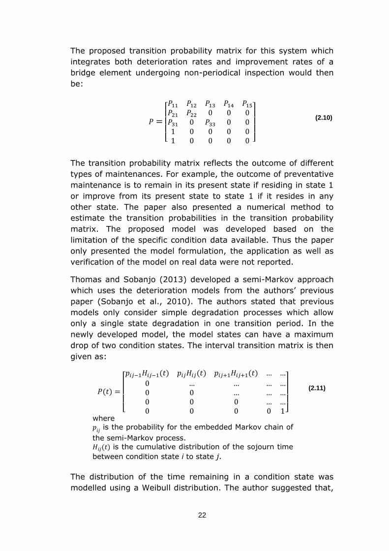
The proposed transition probability matrix for this system which
integrates both deterioration rates and improvement rates of a
bridge element undergoing non-periodical inspection would then
be:
[
]
(2.10)
The transition probability matrix reflects the outcome of different
types of maintenances. For example, the outcome of preventative
maintenance is to remain in its present state if residing in state 1
or improve from its present state to state 1 if it resides in any
other state. The paper also presented a numerical method to
estimate the transition probabilities in the transition probability
matrix. The proposed model was developed based on the
limitation of the specific condition data available. Thus the paper
only presented the model formulation, the application as well as
verification of the model on real data were not reported.
Thomas and Sobanjo (2013) developed a semi-Markov approach
which uses the deterioration models from the authors’ previous
paper (Sobanjo et al., 2010). The authors stated that previous
models only consider simple degradation processes which allow
only a single state degradation in one transition period. In the
newly developed model, the model states can have a maximum
drop of two condition states. The interval transition matrix is then
given as:
( )
[ ( ) ( ) ( )
]
(2.11)
where is the probability for the embedded Markov chain of
the semi-Markov process.
( ) is the cumulative distribution of the sojourn time
between condition state i to state j.
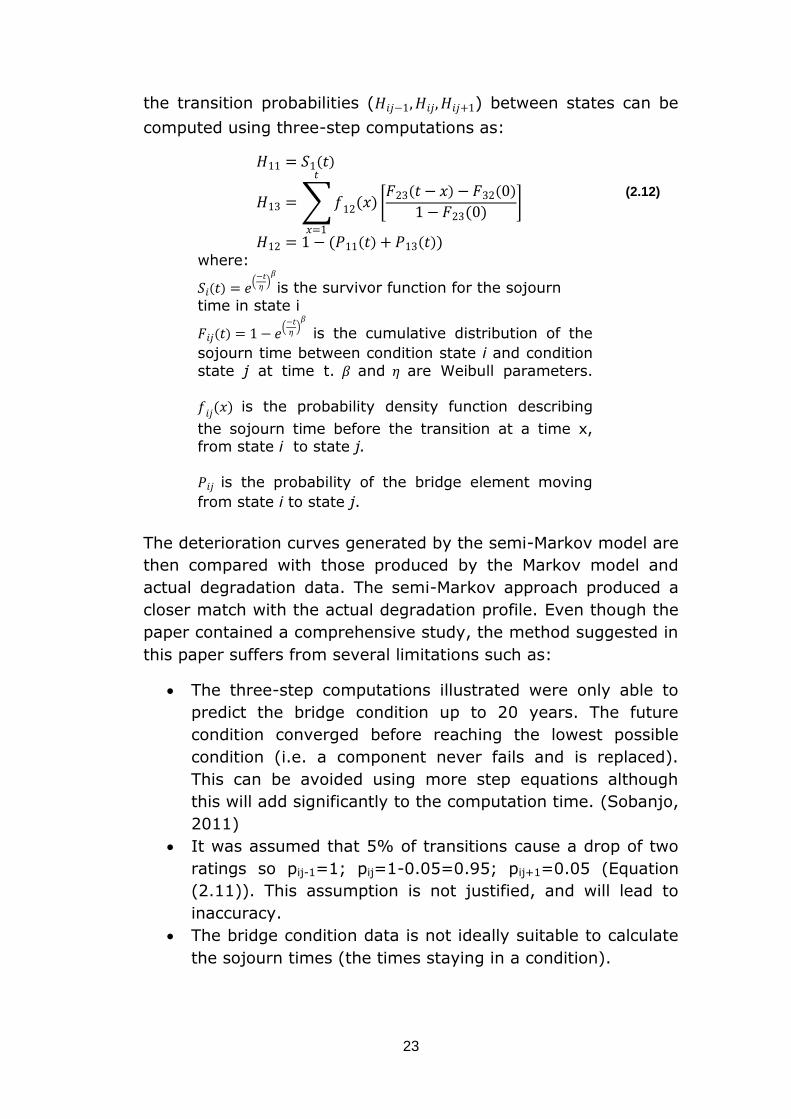
The distribution of the time remaining in a condition state was
modelled using a Weibull distribution. The author suggested that,
23
the transition probabilities ( ) between states can be
computed using three-step computations as:
( )
∑ ( ) [ ( ) ( )
( )]
( ( ) ( ))
(2.12)
where:
( ) (
)
is the survivor function for the sojourn
time in state i
( ) (
)
is the cumulative distribution of the
sojourn time between condition state i and condition
state j at time t. and are Weibull parameters.
( ) is the probability density function describing
the sojourn time before the transition at a time x, from state i to state j.
is the probability of the bridge element moving
from state i to state j.
The deterioration curves generated by the semi-Markov model are
then compared with those produced by the Markov model and
actual degradation data. The semi-Markov approach produced a
closer match with the actual degradation profile. Even though the
paper contained a comprehensive study, the method suggested in
this paper suffers from several limitations such as:
The three-step computations illustrated were only able to
predict the bridge condition up to 20 years. The future
condition converged before reaching the lowest possible
condition (i.e. a component never fails and is replaced).
This can be avoided using more step equations although
this will add significantly to the computation time. (Sobanjo,
2011)
It was assumed that 5% of transitions cause a drop of two
ratings so pij-1=1; pij=1-0.05=0.95; pij+1=0.05 (Equation
(2.11)). This assumption is not justified, and will lead to
inaccuracy.
The bridge condition data is not ideally suitable to calculate
the sojourn times (the times staying in a condition).
24
2.8 Summary and discussion
It was shown that a reasonable amount of research has been
carried out to establish reliable bridge deterioration models over
the last three decades. Markov, semi-Markov and reliability-based
approaches have previously developed for this purpose. The
majority of deterioration models have adapted Markov chain
process in predicting the deterioration process and future
condition of a bridge or a bridge element. There are also a
number of studies based on semi-Markov and reliability-based
approaches, however these studies often lack application and
verification with real data. All of these approaches are able to
capture the stochastic nature of the deterioration process. Thus,
these models predict the future asset condition in terms of the
probability of being in each of the potential states.
Overall, Markov deterioration models have proved to be the most
popular in modelling the bridge asset deterioration process. This
is because the Markov approach is relatively simple to allow a fast
and adequate study using bridge condition data. The model
accounts for the present condition in predicting the future
condition. However, the reviewed models are simple models
which were developed for either one component or for an
individual bridge, not for a bridge system that consist of many
different components. Moreover, the Markov approach suffers
from some limitations such as:
Constant deterioration rates,
The model size increases exponentially with the increasing
number of states (or number of modelled components),
The estimation of the transition probability using regression
method is seriously affected by any prior maintenance
actions (i.e. a rise in condition score) (Ortiz-García et al.,
2006),
The estimation of transition probabilities using the
frequency approach requires: at least two consecutive
condition records without any interventions for a large
number of bridge components at different condition states,
in order to generate reliable transition probabilities (Agrawal
and Kawaguchi, 2009),
The effects of maintenance is not captured i.e. the
degradation process is treated the same before and after
intervention.
25
In contrast to the Markov model, a semi-Markov model often uses
a Weibull distribution to model the time residing in the different
states. Models based on semi-Markov approach are then capable
of using non-constant deterioration rates which overcomes a
major limitation. Though, the approach is based on the Markov-
chain process and still suffers from some similar disadvantages as
in traditional Markov models:
The model size increases exponentially with the increasing
number of states (or number of modelled components),
The estimation of transition probabilities requires
complicated numerical solutions with associated
computation time,
The effects of maintenance is not captured i.e. the
degradation process is treated the same before and after
intervention.
In reliability-based models, the degradation process of bridges or
bridge elements is modelled based on the life time analysis
technique. An appropriate distribution is selected to model the
times of a bridge component reaching a specified condition state.
This approach considers both complete and incomplete lifetime
data. It was demonstrated in all the review studies that the
Weibull distribution is a good fit to these life time data. Also the
obtained distribution parameters obtained indicate a non-constant
i.e. increasing deterioration rates of bridge elements. Although
the method is robust to model the degradation process between
different states, a complete deterioration model comprising of all
component states have not been developed.
All approaches discussed are based on statistical analysis of
condition ratings, however, it is believed that the condition data
used is inadequate for any detailed study of the degradation
characteristic. There are serious limitations associated which
affect the prediction results such as:
Condition data is based on the subjective evaluation by
bridge inspectors with the reliability of the ratings
dependent on the experience of the inspectors (Office of
Rail Regulation, 2007). Moreover, condition rating does not
reflect the structural integrity of a bridge,
Constant periods between inspections means that the data
is collected at fixed intervals, thus the time at which a

26
change in state of the bridge component is experienced is
unknown and is often assumed to occur half way between
inspection interval, this introduces bias variables in the
times to these events thus affects the distribution fitted to
these times,
Condition data does not reflect the effects of maintenance.
Data indicates rises in the score are usually removed. This
means that the effect of maintenance is often ignored.
27
Chapter 3 - Data Analysis and Deterioration Modelling
3.1 Introduction
The research aim is to study the real data to understand the
structure characteristics and the deterioration process. This real
data used in the study was provided by Network Rail, who owns
and operates most of the UK railway infrastructures. It contains
historical maintenance records of the bridge elements, including
the inspection dates and the component condition scores. As
discussed in Chapter 2, the bridge condition score system is
believed to be inadequate to provide a sound study of the bridge
element deterioration process. This chapter presents a novel
method of modelling the asset deterioration process, this involves
constructing a timeline of all historical work done of a bridge
element and analysing the life time of the component reaching
these intervention actions. The analysis methodology will be
presented in detail after the discussion of the available datasets.
Finally, the chapter presents the results obtained from the
analysis.
3.2 Database
There are the five datasets that are used in this research. Table
3.1 shows the size of these datasets and their description as well
as the information that was extracted for the study.
The CARRS dataset contains asset information on the structure
and the work done reports. The dataset was developed in 2007 to
replace multiple local systems currently in operation throughout

28
the railway network (i.e. local databases and spreadsheets) and
to have a single asset management system containing
information of the whole structures asset portfolio. The oldest
record in the CARRS dataset dates back to 1994 until current
date.
The VERA dataset contains structure assessment reports from
1950 up to 2010. These reports contain structural assessments in
term of loading capability, maximum stress, and suggestions
whether if strengthening is required or if the bridge is capable for
running a certain train speed. However only about 37% (12,628
records) of the dataset contains some information, the rest are
blank records.
The SCMI dataset is the biggest database on the bridge structures
and contains very useful information about the minor and major
elements of individual bridge asset. This system was designed by
Network Rail as a high level asset management tool to measure
and demonstrate the change in condition of bridge stock with
time. Bridge components were inspected and rated with a score
between 0–100. There are two key issues that were reported with
this system, they are:
First is the low rate of structures examination. The
company’ standards require a detailed condition survey of
each bridge at a normal interval of 6 years, with the system
starting in 2000, there is only 60% of the bridges were
inspected by 2006-2007. The company is well behind the
inspection programme and this is reflected in this dataset as
most of the structures only contain one set of scores over
the course of 10 years period starting from 2000 up to
current date (Network Rail, 2007a).
Second is the concern expressed, by the Office of Rail
Regulation (ORR), about the accuracy of the score recorded
(Office of Rail Regulation, 2007).
Both of the CAF and MONITOR datasets contains intervention
records with associated costs (expected cost and actual cost) on
bridge asset. The CAF dataset collects information for major
interventions, typically those with an expenditure of over
£50,000. The MONITOR dataset collects information for smaller
interventions with the associated cost of less than £50,000.
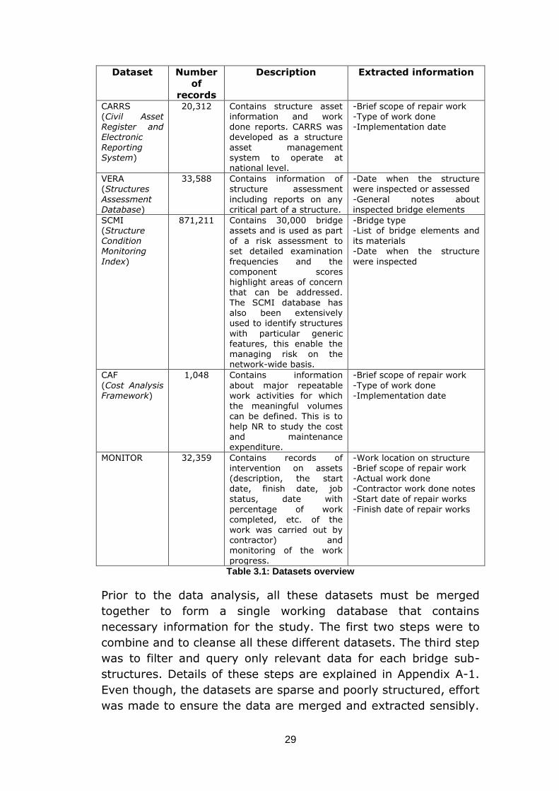
29
Dataset Number
of
records
Description Extracted information
CARRS (Civil Asset Register and Electronic
Reporting System)
20,312 Contains structure asset information and work done reports. CARRS was developed as a structure
asset management system to operate at national level.
-Brief scope of repair work -Type of work done -Implementation date
VERA (Structures
Assessment Database)
33,588 Contains information of structure assessment
including reports on any critical part of a structure.
-Date when the structure were inspected or assessed
-General notes about inspected bridge elements
SCMI (Structure
Condition Monitoring
Index)
871,211 Contains 30,000 bridge assets and is used as part
of a risk assessment to set detailed examination
frequencies and the component scores highlight areas of concern that can be addressed. The SCMI database has also been extensively used to identify structures
with particular generic features, this enable the managing risk on the network-wide basis.
-Bridge type -List of bridge elements and
its materials -Date when the structure
were inspected
CAF
(Cost Analysis Framework)
1,048 Contains information
about major repeatable work activities for which
the meaningful volumes can be defined. This is to help NR to study the cost and maintenance expenditure.
-Brief scope of repair work
-Type of work done -Implementation date
MONITOR 32,359 Contains records of intervention on assets (description, the start date, finish date, job status, date with
percentage of work completed, etc. of the work was carried out by contractor) and monitoring of the work
progress.
-Work location on structure -Brief scope of repair work -Actual work done -Contractor work done notes -Start date of repair works
-Finish date of repair works
Table 3.1: Datasets overview
Prior to the data analysis, all these datasets must be merged
together to form a single working database that contains
necessary information for the study. The first two steps were to
combine and to cleanse all these different datasets. The third step
was to filter and query only relevant data for each bridge sub-
structures. Details of these steps are explained in Appendix A-1.
Even though, the datasets are sparse and poorly structured, effort
was made to ensure the data are merged and extracted sensibly.

30
The final working dataset then contains information about each
individual asset. It contains not only the structure information,
but also the details of the works that have been done, associated
costs, previous inspection, and any other work related records. All
of these information fields in the working database are illustrated
in Figure 3.1. It is worth mentioning that with the issues
associated with the SCMI score, this data was not studied in this
research. The research focuses mainly on historical maintenance
data to study the degradation process of an asset.
Figure 3.1: Information fields in a single working database after the merging and cleansing of all different datasets
3.2.1 Data problems and assumptions
Large amount of data was not recorded in descriptive words
but rather sentences or paragraphs, information was
extracted from these data by reading through each record
manually.
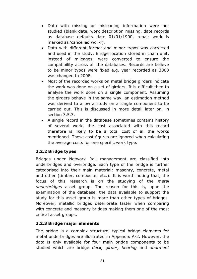
31
Data with missing or misleading information were not
studied (blank date, work description missing, date records
as database defaults date 01/01/1900, repair work is
marked as ‘cancelled work’).
Data with different format and minor typos was corrected
and used in the study. Bridge location stored in chain unit,
instead of mileages, were converted to ensure the
compatibility across all the databases. Records are believe
to be minor typos were fixed e.g. year recorded as 3008
was changed to 2008.
Most of the recorded works on metal bridge girders indicate
the work was done on a set of girders. It is difficult then to
analyse the work done on a single component. Assuming
the girders behave in the same way, an estimation method
was derived to allow a study on a single component to be
carried out. This is discussed in more detail later on, in
section 3.5.3.
A single record in the database sometimes contains history
of several work, the cost associated with this record
therefore is likely to be a total cost of all the works
mentioned. These cost figures are ignored when calculating
the average costs for one specific work type.
3.2.2 Bridge types
Bridges under Network Rail management are classified into
underbridges and overbridge. Each type of the bridge is further
categorised into their main material: masonry, concrete, metal
and other (timber, composite, etc.). It is worth noting that, the
focus of this research is on the studying of the metal
underbridges asset group. The reason for this is, upon the
examination of the database, the data available to support the
study for this asset group is more than other types of bridges.
Moreover, metallic bridges deteriorate faster when comparing
with concrete and masonry bridges making them one of the most
critical asset groups.
3.2.3 Bridge major elements
The bridge is a complex structure, typical bridge elements for
metal underbridges are illustrated in Appendix A-2. However, the
data is only available for four main bridge components to be
studied which are bridge deck, girder, bearing and abutment
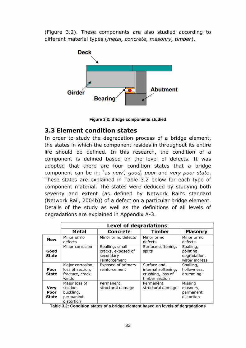
32
(Figure 3.2). These components are also studied according to
different material types (metal, concrete, masonry, timber).
Figure 3.2: Bridge components studied
3.3 Element condition states
In order to study the degradation process of a bridge element,
the states in which the component resides in throughout its entire
life should be defined. In this research, the condition of a
component is defined based on the level of defects. It was
adopted that there are four condition states that a bridge
component can be in: ‘as new’, good, poor and very poor state.
These states are explained in Table 3.2 below for each type of
component material. The states were deduced by studying both
severity and extent (as defined by Network Rail’s standard
(Network Rail, 2004b)) of a defect on a particular bridge element.
Details of the study as well as the definitions of all levels of
degradations are explained in Appendix A-3.
Level of degradations
Metal Concrete Timber Masonry
New Minor or no defects
Minor or no defects Minor or no defects
Minor or no defects
Good State
Minor corrosion
Spalling, small cracks, exposed of secondary
reinforcement
Surface softening, splits
Spalling, pointing degradation,
water ingress
Poor State
Major corrosion, loss of section, fracture, crack welds
Exposed of primary reinforcement
Surface and internal softening, crushing, loss of timber section
Spalling, hollowness, drumming
Very Poor State
Major loss of section, buckling, permanent distortion
Permanent structural damage
Permanent structural damage
Missing masonry, permanent distortion
Table 3.2: Condition states of a bridge element based on levels of degradations
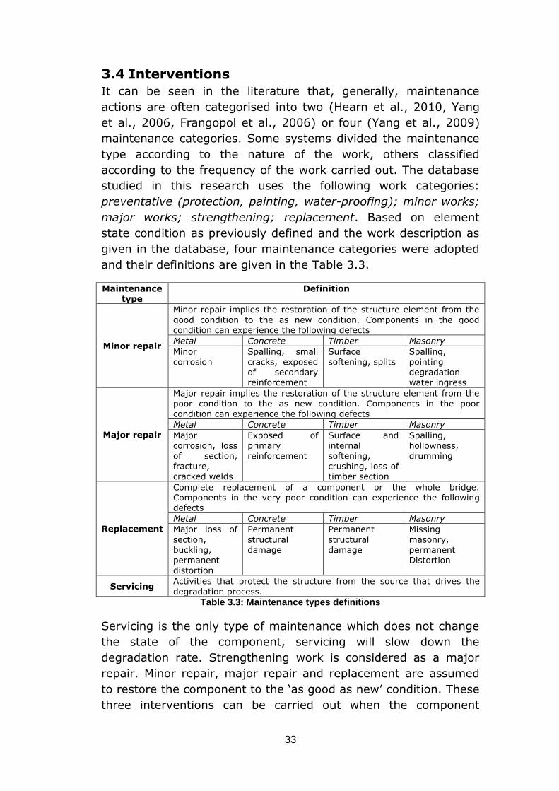
33
3.4 Interventions
It can be seen in the literature that, generally, maintenance
actions are often categorised into two (Hearn et al., 2010, Yang
et al., 2006, Frangopol et al., 2006) or four (Yang et al., 2009)
maintenance categories. Some systems divided the maintenance
type according to the nature of the work, others classified
according to the frequency of the work carried out. The database
studied in this research uses the following work categories:
preventative (protection, painting, water-proofing); minor works;
major works; strengthening; replacement. Based on element
state condition as previously defined and the work description as
given in the database, four maintenance categories were adopted
and their definitions are given in the Table 3.3.
Maintenance type
Definition
Minor repair
Minor repair implies the restoration of the structure element from the good condition to the as new condition. Components in the good condition can experience the following defects
Metal Concrete Timber Masonry
Minor corrosion
Spalling, small cracks, exposed of secondary reinforcement
Surface softening, splits
Spalling, pointing degradation water ingress
Major repair
Major repair implies the restoration of the structure element from the
poor condition to the as new condition. Components in the poor condition can experience the following defects
Metal Concrete Timber Masonry
Major corrosion, loss of section, fracture, cracked welds
Exposed of primary reinforcement
Surface and internal softening, crushing, loss of timber section
Spalling, hollowness, drumming
Replacement
Complete replacement of a component or the whole bridge. Components in the very poor condition can experience the following defects
Metal Concrete Timber Masonry
Major loss of
section, buckling,
permanent distortion
Permanent
structural damage
Permanent
structural damage
Missing
masonry, permanent
Distortion
Servicing Activities that protect the structure from the source that drives the
degradation process.
Table 3.3: Maintenance types definitions
Servicing is the only type of maintenance which does not change
the state of the component, servicing will slow down the
degradation rate. Strengthening work is considered as a major
repair. Minor repair, major repair and replacement are assumed
to restore the component to the ‘as good as new’ condition. These
three interventions can be carried out when the component
34
reaches the good, poor or very poor state from the ‘as new’
condition.
3.5 Deterioration modelling
It is important to understand the asset and its component
characteristics in order to develop an accurate asset model.
Different components would experience different level of
degradation and it is desirable to study components in a group
which they share common factors that would cause similar
degradation process. In other words, the study should be carried
out on a group of components that have the same structure,
material, environment, route criticality, traffic tonnage.
Unfortunately, the information available were not enough for such
detailed study, hence the components are grouped in term of
structure and material for the degradation analysis.
3.5.1 Life time data
The degradation of a bridge element is analysed by studying the
historical maintenance records throughout its lifetime. Typical
deterioration pattern can be seen in Figure 3.3. The time to reach
state j and k from new (state i) are given as and
. These
times are often called the time to failure and the term ‘failure’
used here does not mean the physical failure of a component but
indicates the time to the point when a certain type of repair is
necessary. It is important when analysing the lifetime data of a
component to account for both complete data, and censored
data, . Complete data indicates the time of reaching state k
from the new condition. Censored data is incomplete data where
it has not been possible to measure the full lifetime. This may be
because the component was repaired or replaced, for some
reason, prior to reaching the condition k and so the full life has
not been observed. The components life is however known to be
at least . Figure 3.3 shows how the complete and censored
time were being analysed. The time between major repair and
minor repair is a complete time indicates the full life time of the
component reaching the state where minor repair is required from
the ‘as new’ state. This time is also the censored time indicates
the component’s condition was restored to new condition before it
reaches the state where major repair is necessary hence the full
time between two major repairs cannot be measured. In the case
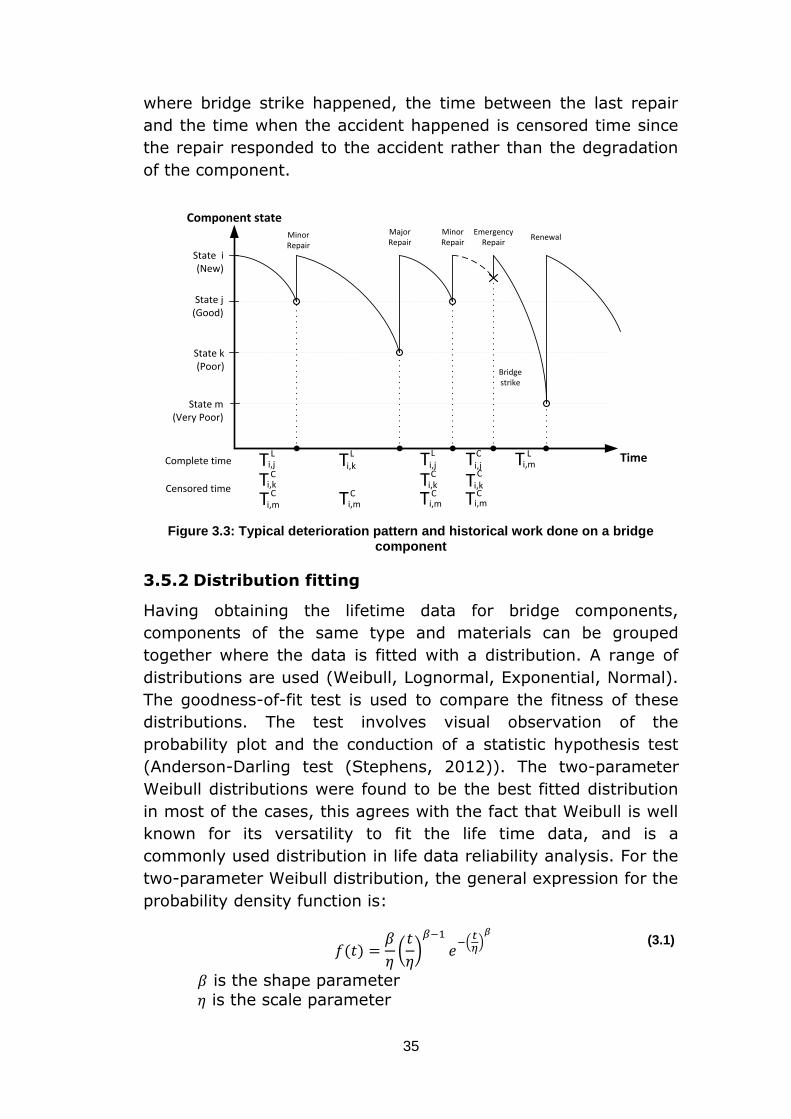
35
where bridge strike happened, the time between the last repair
and the time when the accident happened is censored time since
the repair responded to the accident rather than the degradation
of the component.
Component state
Time
Minor Repair
State i(New)
State j(Good)
State k(Poor)
Minor Repair
Emergency Repair
Major Repair
T Li,j TL
i,k T Li,mTL
i,j TCi,j
Renewal
TCi,k
Complete time
Censored timeT C
i,k TC
i,k
State m(Very Poor)
T Ci,m T C
i,mTCi,m TC
i,m
Bridge strike
Figure 3.3: Typical deterioration pattern and historical work done on a bridge
component
3.5.2 Distribution fitting
Having obtaining the lifetime data for bridge components,
components of the same type and materials can be grouped
together where the data is fitted with a distribution. A range of
distributions are used (Weibull, Lognormal, Exponential, Normal).
The goodness-of-fit test is used to compare the fitness of these
distributions. The test involves visual observation of the
probability plot and the conduction of a statistic hypothesis test
(Anderson-Darling test (Stephens, 2012)). The two-parameter
Weibull distributions were found to be the best fitted distribution
in most of the cases, this agrees with the fact that Weibull is well
known for its versatility to fit the life time data, and is a
commonly used distribution in life data reliability analysis. For the
two-parameter Weibull distribution, the general expression for the
probability density function is:
( )
(
)
(
)
(3.1)
is the shape parameter
is the scale parameter
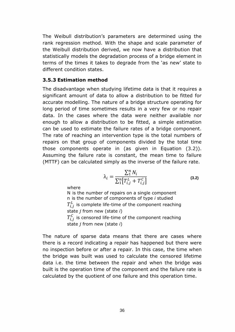
36
The Weibull distribution’s parameters are determined using the
rank regression method. With the shape and scale parameter of
the Weibull distribution derived, we now have a distribution that
statistically models the degradation process of a bridge element in
terms of the times it takes to degrade from the ‘as new’ state to
different condition states.
3.5.3 Estimation method
The disadvantage when studying lifetime data is that it requires a
significant amount of data to allow a distribution to be fitted for
accurate modelling. The nature of a bridge structure operating for
long period of time sometimes results in a very few or no repair
data. In the cases where the data were neither available nor
enough to allow a distribution to be fitted, a simple estimation
can be used to estimate the failure rates of a bridge component.
The rate of reaching an intervention type is the total numbers of
repairs on that group of components divided by the total time
those components operate in (as given in Equation (3.2)).
Assuming the failure rate is constant, the mean time to failure
(MTTF) can be calculated simply as the inverse of the failure rate.
∑
∑ [
]
(3.2)
where N is the number of repairs on a single component n is the number of components of type i studied
is complete life-time of the component reaching
state j from new (state i)
is censored life-time of the component reaching
state j from new (state i)
The nature of sparse data means that there are cases where
there is a record indicating a repair has happened but there were
no inspection before or after a repair. In this case, the time when
the bridge was built was used to calculate the censored lifetime
data i.e. the time between the repair and when the bridge was
built is the operation time of the component and the failure rate is
calculated by the quotient of one failure and this operation time.
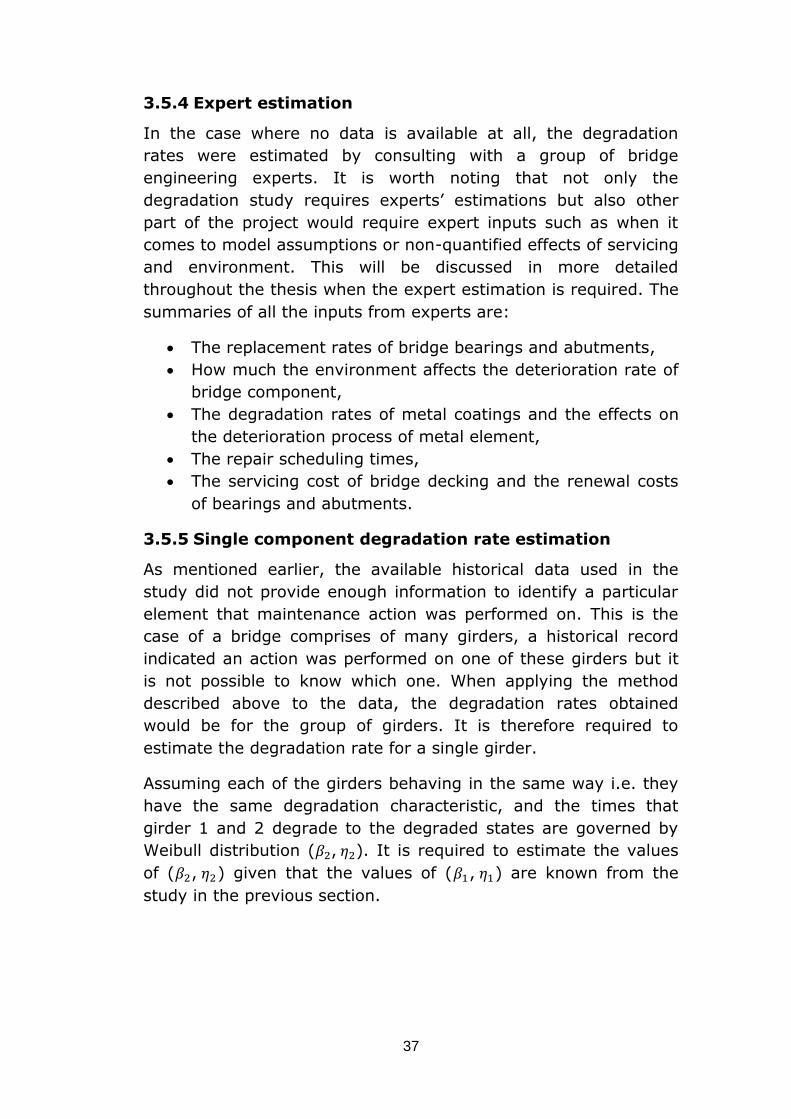
37
3.5.4 Expert estimation
In the case where no data is available at all, the degradation
rates were estimated by consulting with a group of bridge
engineering experts. It is worth noting that not only the
degradation study requires experts’ estimations but also other
part of the project would require expert inputs such as when it
comes to model assumptions or non-quantified effects of servicing
and environment. This will be discussed in more detailed
throughout the thesis when the expert estimation is required. The
summaries of all the inputs from experts are:
The replacement rates of bridge bearings and abutments,
How much the environment affects the deterioration rate of
bridge component,
The degradation rates of metal coatings and the effects on
the deterioration process of metal element,
The repair scheduling times,
The servicing cost of bridge decking and the renewal costs
of bearings and abutments.
3.5.5 Single component degradation rate estimation
As mentioned earlier, the available historical data used in the
study did not provide enough information to identify a particular
element that maintenance action was performed on. This is the
case of a bridge comprises of many girders, a historical record
indicated an action was performed on one of these girders but it
is not possible to know which one. When applying the method
described above to the data, the degradation rates obtained
would be for the group of girders. It is therefore required to
estimate the degradation rate for a single girder.
Assuming each of the girders behaving in the same way i.e. they
have the same degradation characteristic, and the times that
girder 1 and 2 degrade to the degraded states are governed by
Weibull distribution ( , ). It is required to estimate the values
of ( , ) given that the values of ( , ) are known from the
study in the previous section.
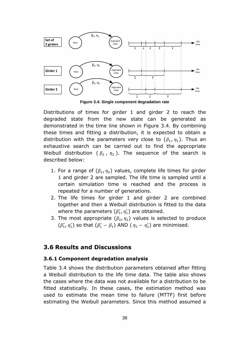
38
Figure 3.4: Single component degradation rate
Distributions of times for girder 1 and girder 2 to reach the
degraded state from the new state can be generated as
demonstrated in the time line shown in Figure 3.4. By combining
these times and fitting a distribution, it is expected to obtain a
distribution with the parameters very close to ( , ). Thus an
exhaustive search can be carried out to find the appropriate
Weibull distribution ( , ). The sequence of the search is
described below:
1. For a range of ( , ) values, complete life times for girder
1 and girder 2 are sampled. The life time is sampled until a
certain simulation time is reached and the process is
repeated for a number of generations.
2. The life times for girder 1 and girder 2 are combined
together and then a Weibull distribution is fitted to the data
where the parameters ( ,
) are obtained.
3. The most appropriate ( , ) values is selected to produce
( ,
) so that ( ) AND (
) are minimised.
3.6 Results and Discussions
3.6.1 Component degradation analysis
Table 3.4 shows the distribution parameters obtained after fitting
a Weibull distribution to the life time data. The table also shows
the cases where the data was not available for a distribution to be
fitted statistically. In these cases, the estimation method was
used to estimate the mean time to failure (MTTF) first before
estimating the Weibull parameters. Since this method assumed a
NewDegraded
state
NewDegraded
state
NewDegraded
state
β2, η2
β2, η2
β1, η1
Set of 2 girders
Girder 1
Girder 2
Life time
Life time
Life time
F F F
F F
F F F F F
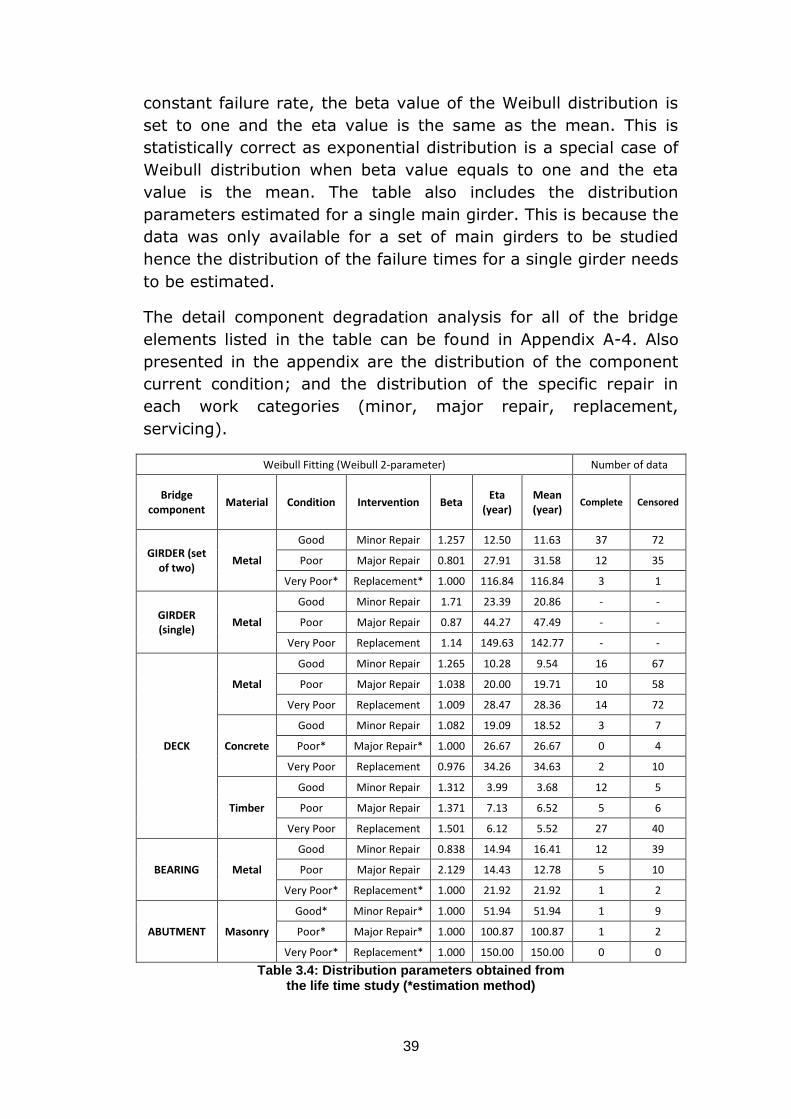
39
constant failure rate, the beta value of the Weibull distribution is
set to one and the eta value is the same as the mean. This is
statistically correct as exponential distribution is a special case of
Weibull distribution when beta value equals to one and the eta
value is the mean. The table also includes the distribution
parameters estimated for a single main girder. This is because the
data was only available for a set of main girders to be studied
hence the distribution of the failure times for a single girder needs
to be estimated.
The detail component degradation analysis for all of the bridge
elements listed in the table can be found in Appendix A-4. Also
presented in the appendix are the distribution of the component
current condition; and the distribution of the specific repair in
each work categories (minor, major repair, replacement,
servicing).
Weibull Fitting (Weibull 2-parameter) Number of data
Bridge component
Material Condition Intervention Beta Eta
(year) Mean (year)
Complete Censored
GIRDER (set of two)
Metal
Good Minor Repair 1.257 12.50 11.63 37 72
Poor Major Repair 0.801 27.91 31.58 12 35
Very Poor* Replacement* 1.000 116.84 116.84 3 1
GIRDER (single)
Metal
Good Minor Repair 1.71 23.39 20.86 - -
Poor Major Repair 0.87 44.27 47.49 - -
Very Poor Replacement 1.14 149.63 142.77 - -
DECK
Metal
Good Minor Repair 1.265 10.28 9.54 16 67
Poor Major Repair 1.038 20.00 19.71 10 58
Very Poor Replacement 1.009 28.47 28.36 14 72
Concrete
Good Minor Repair 1.082 19.09 18.52 3 7
Poor* Major Repair* 1.000 26.67 26.67 0 4
Very Poor Replacement 0.976 34.26 34.63 2 10
Timber
Good Minor Repair 1.312 3.99 3.68 12 5
Poor Major Repair 1.371 7.13 6.52 5 6
Very Poor Replacement 1.501 6.12 5.52 27 40
BEARING Metal
Good Minor Repair 0.838 14.94 16.41 12 39
Poor Major Repair 2.129 14.43 12.78 5 10
Very Poor* Replacement* 1.000 21.92 21.92 1 2
ABUTMENT Masonry
Good* Minor Repair* 1.000 51.94 51.94 1 9
Poor* Major Repair* 1.000 100.87 100.87 1 2
Very Poor* Replacement* 1.000 150.00 150.00 0 0
Table 3.4: Distribution parameters obtained from the life time study (*estimation method)

40
There are a total of more than 37,000 bridge main girders
component in the whole bridge population. The number of data
contains historical work done are quite low, with only 604 sets of
girders that actually contain useful records. This means that only
1.6% of the population were analysed. The Weibull shape
parameter obtained illustrates that the rate of deteriorating from
a new to a good condition for a main girder is increasing with time
(wear-out characteristics). The failure rate is double after 20
years residing in new state. However the rate of reaching the
poor condition shows unexpected behaviour, it is suspected that
the lack of data has resulted in the decreasing rate of failure with
time. Although there are a significant number of records on minor
and major intervention, there are only 4 entries were recorded for
the renewal of bridge main girders. Moreover, these records were
missing inspection information which prevents the derivation of
the lifetime data. Thus, a distribution could not be fitted to model
the rate of main girders replacement. The estimation method was
employed to estimate the rate of girder replacement.
For metal decks, the shape parameters obtains for a component
reaching the poor and the very poor state are very close to one,
this means that the rate of a component requires major repairs
and replacement is almost constant over time and is about 0.05
and 0.03 metal deck per year. In contrast, the rate of metal
decks moving from new condition to good condition is increasing
from 0.06 metal decks per year to about 0.18 after 60 years.
Thus it is three times more likely to require a minor repair for a
metal deck in 60 years old comparing with the new metal deck.
Almost the entire population of concrete decks are in new and
good conditions with only about 1% of the population is in the
very poor condition that would need replacement. Also due to the
young age of the concrete structure, not many historical data are
available for the study, there were only 10 minor repairs, 4 major
repairs and 12 deck replacements recorded.
Timber deck result demonstrated a very short live comparing with
deckings of other materials. Also the failure rates for reaching
different conditions increase significantly with time. The results
show that the characteristic time for a timber deck to be replaced
is actually faster than the time for it to undergo major repairs.
This suggests that the deck would actually need to be replaced
before it needs major repairs. The reason for this is because

41
timber materials have a short life span, also timber is much
harder to repair. Once the material reaches a point of severe
defects, the timber deck is usually replaced. This preferable
option of repairs is demonstrated by looking at the number of
replacements recorded in the database. The number of
replacements recorded in the database, more than 100 timber
deck replacements, which is much greater than the number of
times major repair were carried out (20 timber deck major
repairs).
The rate at which the bearing would require a minor repair is
almost constant at about 0.1 every year. Unexpectedly, it can be
seen that the characteristic life of the bearing reaching a poor
condition is actually shorter than that of reaching a good
condition. The data that indicates a bearing major repair is often
extracted from an entry that carries information about other
repair works. Even though this entry is categorised in the
database as major work, it might be that other works were major
and the bearing repair might be opportunistic work. About 70% of
bearing major repair data were extracted this way and since it is
not possible to validate these entries, it is accepted that the data
has influence these unexpected results.
The results obtained indicate that the abutment requires much
less maintenance than other bridge elements with the mean time
of an abutment to require minor repair is about 50 years. There
were not enough data to allow the rate of abutment replacement
to be calculated, which again agrees with the fact that abutment
almost never require complete replacement, unless it is a
complete demolition of the entire bridge due to upgrade or
natural disaster.
In general, the distributions of times reaching different states for
all the components suggested that, in most cases, we are
expecting a slightly increasing deterioration rates over time. This
is demonstrated by the beta value of the Weibull distribution is
slightly larger than one.
3.6.2 Servicing effects
When there is no servicing, the deterioration rate is high, the rate
decreases as the servicing interval decreases i.e. servicing more
frequently, though the rate can only be reduced up to a certain
level. To quantify the effects of the servicing on the deterioration
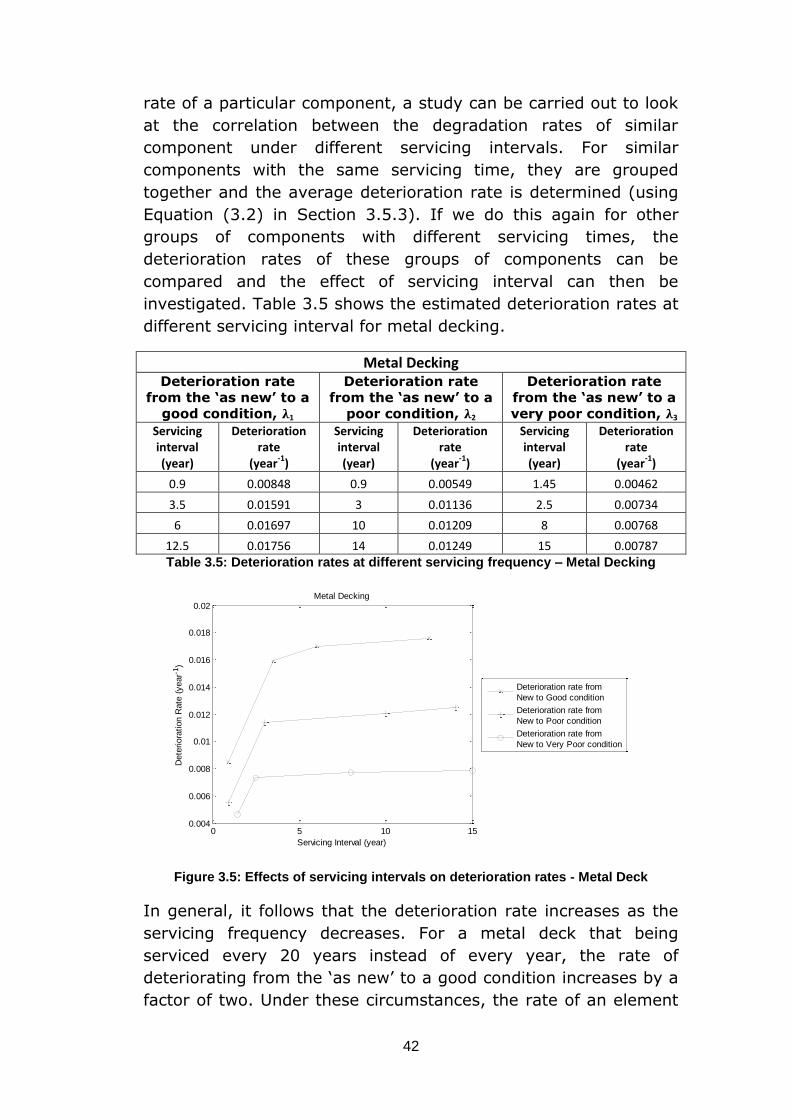
42
rate of a particular component, a study can be carried out to look
at the correlation between the degradation rates of similar
component under different servicing intervals. For similar
components with the same servicing time, they are grouped
together and the average deterioration rate is determined (using
Equation (3.2) in Section 3.5.3). If we do this again for other
groups of components with different servicing times, the
deterioration rates of these groups of components can be
compared and the effect of servicing interval can then be
investigated. Table 3.5 shows the estimated deterioration rates at
different servicing interval for metal decking.
Metal Decking Deterioration rate
from the ‘as new’ to a
good condition, 1
Deterioration rate
from the ‘as new’ to a
poor condition, 2
Deterioration rate
from the ‘as new’ to a
very poor condition, 3
Servicing interval (year)
Deterioration rate
(year-1
)
Servicing interval (year)
Deterioration rate
(year-1
)
Servicing interval (year)
Deterioration rate
(year-1
)
0.9 0.00848 0.9 0.00549 1.45 0.00462
3.5 0.01591 3 0.01136 2.5 0.00734
6 0.01697 10 0.01209 8 0.00768
12.5 0.01756 14 0.01249 15 0.00787 Table 3.5: Deterioration rates at different servicing frequency – Metal Decking
Figure 3.5: Effects of servicing intervals on deterioration rates - Metal Deck
In general, it follows that the deterioration rate increases as the
servicing frequency decreases. For a metal deck that being
serviced every 20 years instead of every year, the rate of
deteriorating from the ‘as new’ to a good condition increases by a
factor of two. Under these circumstances, the rate of an element
0 5 10 150.004
0.006
0.008
0.01
0.012
0.014
0.016
0.018
0.02
Servicing Interval (year)
Dete
riora
tion R
ate
(year-1
)
Metal Decking
Deterioration rate from
New to Good condition
Deterioration rate from
New to Poor condition
Deterioration rate from
New to Very Poor condition
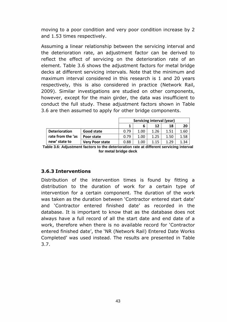
43
moving to a poor condition and very poor condition increase by 2
and 1.53 times respectively.
Assuming a linear relationship between the servicing interval and
the deterioration rate, an adjustment factor can be derived to
reflect the effect of servicing on the deterioration rate of an
element. Table 3.6 shows the adjustment factors for metal bridge
decks at different servicing intervals. Note that the minimum and
maximum interval considered in this research is 1 and 20 years
respectively, this is also considered in practice (Network Rail,
2009). Similar investigations are studied on other components,
however, except for the main girder, the data was insufficient to
conduct the full study. These adjustment factors shown in Table
3.6 are then assumed to apply for other bridge components.
Servicing interval (year)
1 6 12 18 20
Deterioration rate from the ‘as new’ state to
Good state 0.79 1.00 1.26 1.51 1.60
Poor state 0.79 1.00 1.25 1.50 1.58
Very Poor state 0.88 1.00 1.15 1.29 1.34 Table 3.6: Adjustment factors to the deterioration rate at different servicing interval
for metal bridge deck
3.6.3 Interventions
Distribution of the intervention times is found by fitting a
distribution to the duration of work for a certain type of
intervention for a certain component. The duration of the work
was taken as the duration between ‘Contractor entered start date’
and ‘Contractor entered finished date’ as recorded in the
database. It is important to know that as the database does not
always have a full record of all the start date and end date of a
work, therefore when there is no available record for ‘Contractor
entered finished date’, the ‘NR (Network Rail) Entered Date Works
Completed’ was used instead. The results are presented in Table
3.7.
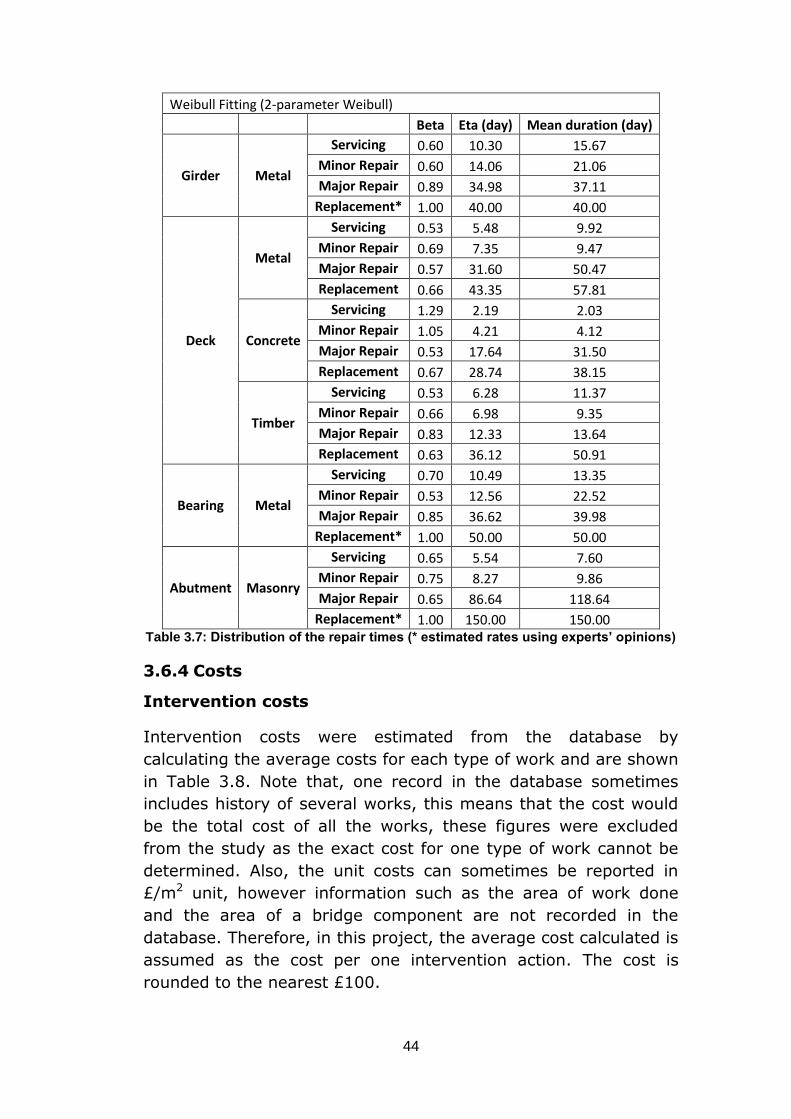
44
Weibull Fitting (2-parameter Weibull)
Beta Eta (day) Mean duration (day)
Girder Metal
Servicing 0.60 10.30 15.67
Minor Repair 0.60 14.06 21.06
Major Repair 0.89 34.98 37.11
Replacement* 1.00 40.00 40.00
Deck
Metal
Servicing 0.53 5.48 9.92
Minor Repair 0.69 7.35 9.47
Major Repair 0.57 31.60 50.47
Replacement 0.66 43.35 57.81
Concrete
Servicing 1.29 2.19 2.03
Minor Repair 1.05 4.21 4.12
Major Repair 0.53 17.64 31.50
Replacement 0.67 28.74 38.15
Timber
Servicing 0.53 6.28 11.37
Minor Repair 0.66 6.98 9.35
Major Repair 0.83 12.33 13.64
Replacement 0.63 36.12 50.91
Bearing Metal
Servicing 0.70 10.49 13.35
Minor Repair 0.53 12.56 22.52
Major Repair 0.85 36.62 39.98
Replacement* 1.00 50.00 50.00
Abutment Masonry
Servicing 0.65 5.54 7.60
Minor Repair 0.75 8.27 9.86
Major Repair 0.65 86.64 118.64
Replacement* 1.00 150.00 150.00 Table 3.7: Distribution of the repair times (* estimated rates using experts’ opinions)
3.6.4 Costs
Intervention costs
Intervention costs were estimated from the database by
calculating the average costs for each type of work and are shown
in Table 3.8. Note that, one record in the database sometimes
includes history of several works, this means that the cost would
be the total cost of all the works, these figures were excluded
from the study as the exact cost for one type of work cannot be
determined. Also, the unit costs can sometimes be reported in
£/m2 unit, however information such as the area of work done
and the area of a bridge component are not recorded in the
database. Therefore, in this project, the average cost calculated is
assumed as the cost per one intervention action. The cost is
rounded to the nearest £100.
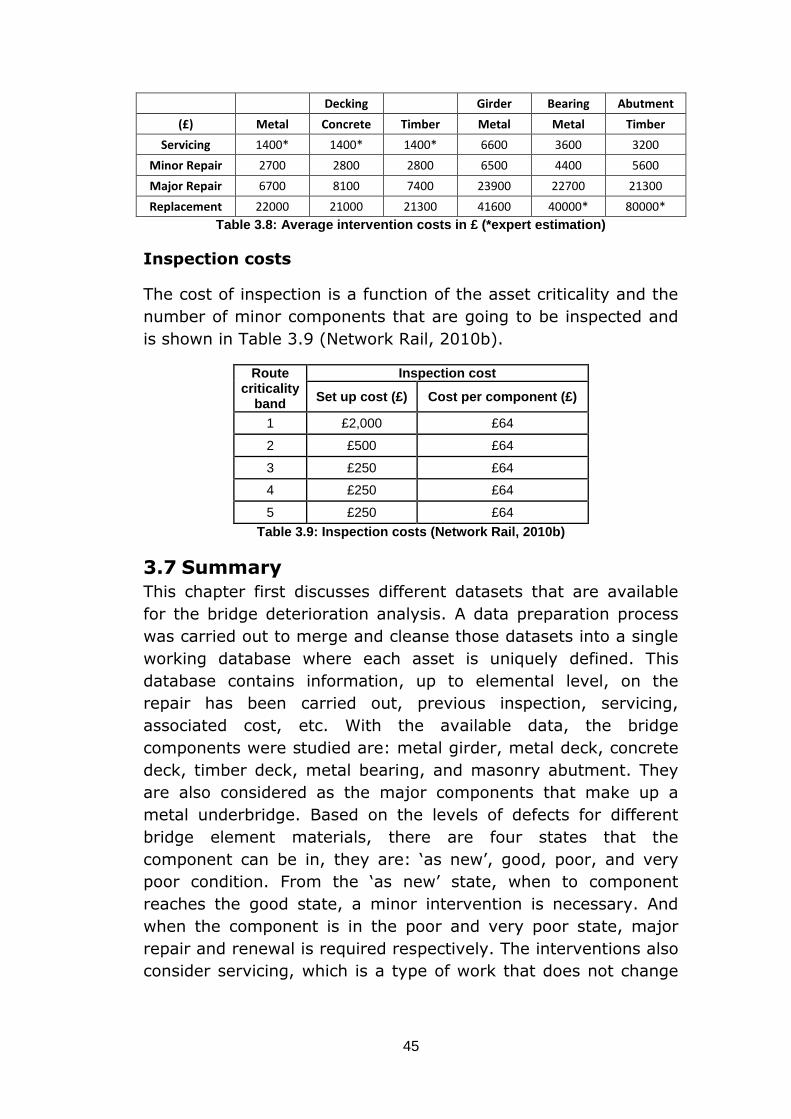
45
Decking
Girder Bearing Abutment
(£) Metal Concrete Timber Metal Metal Timber
Servicing 1400* 1400* 1400* 6600 3600 3200
Minor Repair 2700 2800 2800 6500 4400 5600
Major Repair 6700 8100 7400 23900 22700 21300
Replacement 22000 21000 21300 41600 40000* 80000*
Table 3.8: Average intervention costs in £ (*expert estimation)
Inspection costs
The cost of inspection is a function of the asset criticality and the
number of minor components that are going to be inspected and
is shown in Table 3.9 (Network Rail, 2010b).
Route criticality
band
Inspection cost
Set up cost (£) Cost per component (£)
1 £2,000 £64
2 £500 £64
3 £250 £64
4 £250 £64
5 £250 £64
Table 3.9: Inspection costs (Network Rail, 2010b)
3.7 Summary
This chapter first discusses different datasets that are available
for the bridge deterioration analysis. A data preparation process
was carried out to merge and cleanse those datasets into a single
working database where each asset is uniquely defined. This
database contains information, up to elemental level, on the
repair has been carried out, previous inspection, servicing,
associated cost, etc. With the available data, the bridge
components were studied are: metal girder, metal deck, concrete
deck, timber deck, metal bearing, and masonry abutment. They
are also considered as the major components that make up a
metal underbridge. Based on the levels of defects for different
bridge element materials, there are four states that the
component can be in, they are: ‘as new’, good, poor, and very
poor condition. From the ‘as new’ state, when to component
reaches the good state, a minor intervention is necessary. And
when the component is in the poor and very poor state, major
repair and renewal is required respectively. The interventions also
consider servicing, which is a type of work that does not change
46
the state of the component but slows down the deterioration
rates.
The chapter also presented a method of modelling the
degradation of a bridge element by analysing its historical
maintenance records. A life time of the component is calculated
by the time the component takes to deteriorate from the ‘as new’
state to the state where an intervention was carried out. By
gathering the lifetime for the component of the same type, a
Weibull distribution is fitted to these data to statistically model
the deterioration process. Where there is a little data available,
the estimation method is used, and where there is no data
available, estimation uses the experts’ opinions. In the case
where the degradation process was determined for a group of
main girders, the simulation method of obtaining the distribution
of lifetimes for a single girder was also described. The presented
method demonstrates that ‘life data’ analysis method can be
applied to model the deterioration process of bridge elements.
This method recognises the ‘censored’ nature of bridge lifetime
data and incorporates these data into the deterioration modelling
process.
The distributions of the lifetimes for all bridge major components
were obtained (Table 3.4). The results suggested that, for most of
the cases, the deterioration rates of the components increase
slightly over time. The study also confirmed the effect of the
servicing on the slowing down of the deterioration rate,
component is expect to deteriorate two times as fast when it is
being serviced every 20 years comparing with one is serviced
every year. The distributions of the repair times and the
associated costs were also determined and the results were
reported. All of these results would then be used later on in this
research as the inputs for the bridge model.
Throughout the degradation study, several key problems and
assumptions with the datasets were discussed. The availability as
well as validity of the data has imposed a lot of constraints on the
accurate modelling of the degradation rate with the proposed
method. The degradation study also assumed ‘perfect
maintenance’ i.e. an intervention restores the bridge component’s
condition back to an ‘as good as new’ condition. However with the
demonstrated method, it is expected for more accurate results
with the increasing number and better recorded data.
47
Chapter 4 - Markov Bridge Model
4.1 Introduction
The modelling of the bridge degradation using the Markov
modelling technique has been widely adopted over the last 20
years. There are many Markov bridge models in the literature as
discussed in chapter 2. However, most of these models are
simple. In this chapter, a Markov bridge model is developed that
uses the degradation rates determined from the previous chapter
to model the future asset condition. The model is considered in
much more detail than other bridge models available in the
literature by accounting for the inspection, servicing interval,
repair delay time and opportunistic maintenance. The model can
also be used to investigate the effects of different maintenance
strategies. The whole life cycle costs can also be estimated using
the model.
4.2 Development of the continuous-time Markov
bridge model
4.2.1 Elemental model
4.2.1.1 Degradation process
As discussed in the previous chapter, there are four states a
bridge component can be considered to reside in. Figure 4.1
shows a four-state Markov diagram that models the degradation
process of a single bridge element. In order to satisfy the
Markovian property, the distribution of time transitioning between
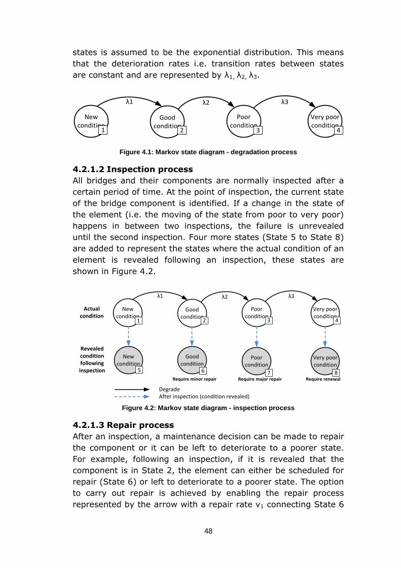
48
states is assumed to be the exponential distribution. This means
that the deterioration rates i.e. transition rates between states
are constant and are represented by λ1, λ2, λ3.
New condition
Good condition
Poor condition
Very poor condition
λ1 λ2
1 2 3 4
λ3
Figure 4.1: Markov state diagram - degradation process
4.2.1.2 Inspection process
All bridges and their components are normally inspected after a
certain period of time. At the point of inspection, the current state
of the bridge component is identified. If a change in the state of
the element (i.e. the moving of the state from poor to very poor)
happens in between two inspections, the failure is unrevealed
until the second inspection. Four more states (State 5 to State 8)
are added to represent the states where the actual condition of an
element is revealed following an inspection, these states are
shown in Figure 4.2.
Require renewalRequire major repairRequire minor repair
New condition
Good condition
Poor condition
Very poor condition
λ1 λ2
Good condition
Poor condition
Very poor condition
1 2
6
3
7 8
4
After inspection (condition revealed)Degrade
λ3
New condition
5
Actual condition
Revealed condition following inspection
Figure 4.2: Markov state diagram - inspection process
4.2.1.3 Repair process
After an inspection, a maintenance decision can be made to repair
the component or it can be left to deteriorate to a poorer state.
For example, following an inspection, if it is revealed that the
component is in State 2, the element can either be scheduled for
repair (State 6) or left to deteriorate to a poorer state. The option
to carry out repair is achieved by enabling the repair process
represented by the arrow with a repair rate ν1 connecting State 6
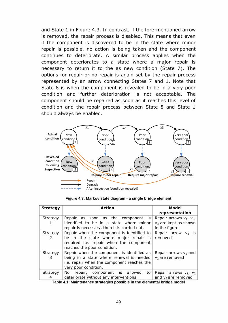
49
and State 1 in Figure 4.3. In contrast, if the fore-mentioned arrow
is removed, the repair process is disabled. This means that even
if the component is discovered to be in the state where minor
repair is possible, no action is being taken and the component
continues to deteriorate. A similar process applies when the
component deteriorates to a state where a major repair is
necessary to return it to the as new condition (State 7). The
options for repair or no repair is again set by the repair process
represented by an arrow connecting States 7 and 1. Note that
State 8 is when the component is revealed to be in a very poor
condition and further deterioration is not acceptable. The
component should be repaired as soon as it reaches this level of
condition and the repair process between State 8 and State 1
should always be enabled.
New condition
Good condition
Poor condition
Very poor condition
λ1 λ2
ν2ν3
Good condition
Poor condition
Very poor condition
ν1
1 2
6
3
7 8
4
After inspection (condition revealed)
RepairDegrade
λ3
New condition
5
Require renewalRequire major repairRequire minor repair
Actual condition
Revealed condition following inspection
Figure 4.3: Markov state diagram - a single bridge element
Strategy Action Model
representation
Strategy
1
Repair as soon as the component is
identified to be in a state where minor
repair is necessary, then it is carried out.
Repair arrows ν1, ν2,
ν3 are kept as shown
in the figure
Strategy
2
Repair when the component is identified to
be in the state where major repair is
required i.e. repair when the component
reaches the poor condition.
Repair arrow ν1 is
removed
Strategy
3
Repair when the component is identified as
being in a state where renewal is needed
i.e. repair when the component reaches the
very poor condition.
Repair arrows ν1 and
ν2 are removed
Strategy
4
No repair, component is allowed to
deteriorate without any interventions
Repair arrows ν1, ν2
and ν3 are removed
Table 4.1: Maintenance strategies possible in the elemental bridge model
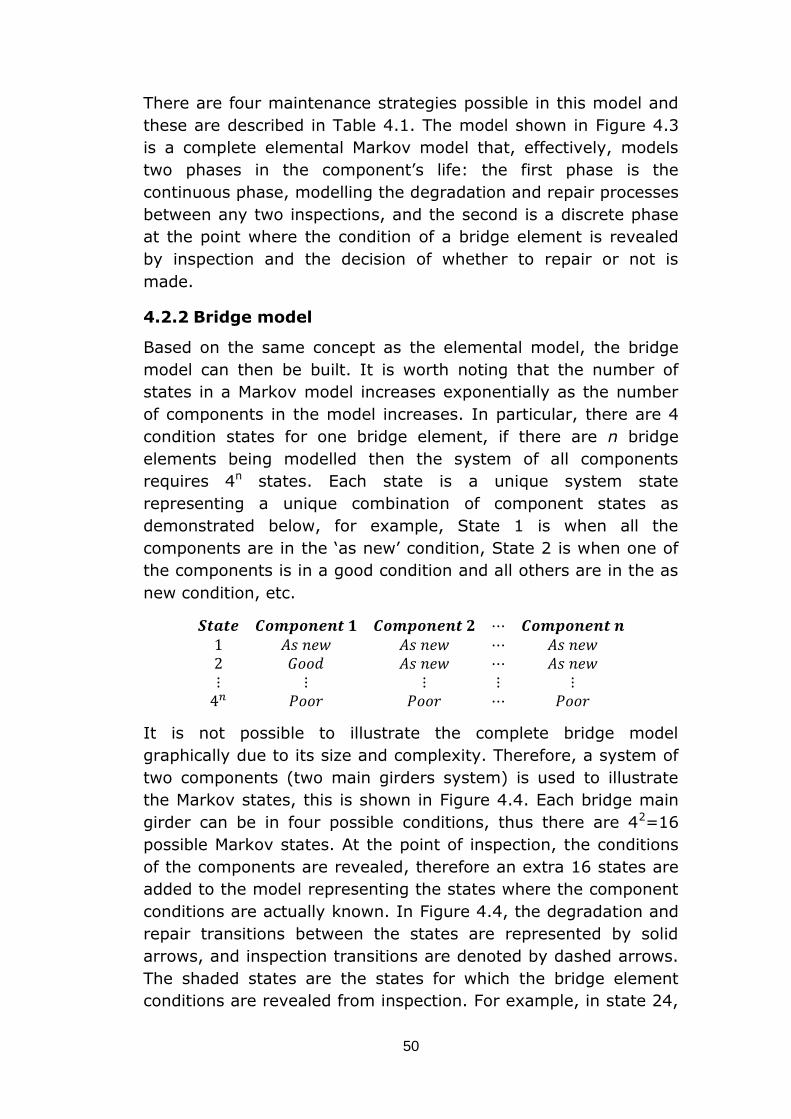
50
There are four maintenance strategies possible in this model and
these are described in Table 4.1. The model shown in Figure 4.3
is a complete elemental Markov model that, effectively, models
two phases in the component’s life: the first phase is the
continuous phase, modelling the degradation and repair processes
between any two inspections, and the second is a discrete phase
at the point where the condition of a bridge element is revealed
by inspection and the decision of whether to repair or not is
made.
4.2.2 Bridge model
Based on the same concept as the elemental model, the bridge
model can then be built. It is worth noting that the number of
states in a Markov model increases exponentially as the number
of components in the model increases. In particular, there are 4
condition states for one bridge element, if there are n bridge
elements being modelled then the system of all components
requires 4n states. Each state is a unique system state
representing a unique combination of component states as
demonstrated below, for example, State 1 is when all the
components are in the ‘as new’ condition, State 2 is when one of
the components is in a good condition and all others are in the as
new condition, etc.
It is not possible to illustrate the complete bridge model
graphically due to its size and complexity. Therefore, a system of
two components (two main girders system) is used to illustrate
the Markov states, this is shown in Figure 4.4. Each bridge main
girder can be in four possible conditions, thus there are 42=16
possible Markov states. At the point of inspection, the conditions
of the components are revealed, therefore an extra 16 states are
added to the model representing the states where the component
conditions are actually known. In Figure 4.4, the degradation and
repair transitions between the states are represented by solid
arrows, and inspection transitions are denoted by dashed arrows.
The shaded states are the states for which the bridge element
conditions are revealed from inspection. For example, in state 24,

51
it is revealed that after the inspection, the main girder 1 (G1) is in
a good (G) condition while the main girder 2 (G2) is in a very
poor (VP) condition.
If the maintenance strategy is to repair the components as soon
as they reach a state where repair is possible, then the repair
process will restore the girders’ conditions to ‘as good as new’.
This is represented by the repair process from state 24 to state 1.
It is worth noting that for different maintenance strategies, the
Markov model states are the same however the repair transitions
are different. Figure 4.5 and Figure 4.6 illustrate the model for
the same two girder system that is managed under maintenance
strategies 2 and 3 respectively. Note that the degradation
transitions are the same as illustrated in Figure 4.4 and are not
therefore shown in those figures for the sake of clarity.
A computer program was written in Matlab to aid the process of
generating the larger and more detailed Markov bridge model to
include more components. The software first generates all the
possible model states then generates all the transitions possible
governed by a specified maintenance strategy. The software
allows the model of any size to be generated, thus the size of the
model is only restricted by the memory size available on a
particular machine. However, the solution time increases
significantly as the size of the model increases.
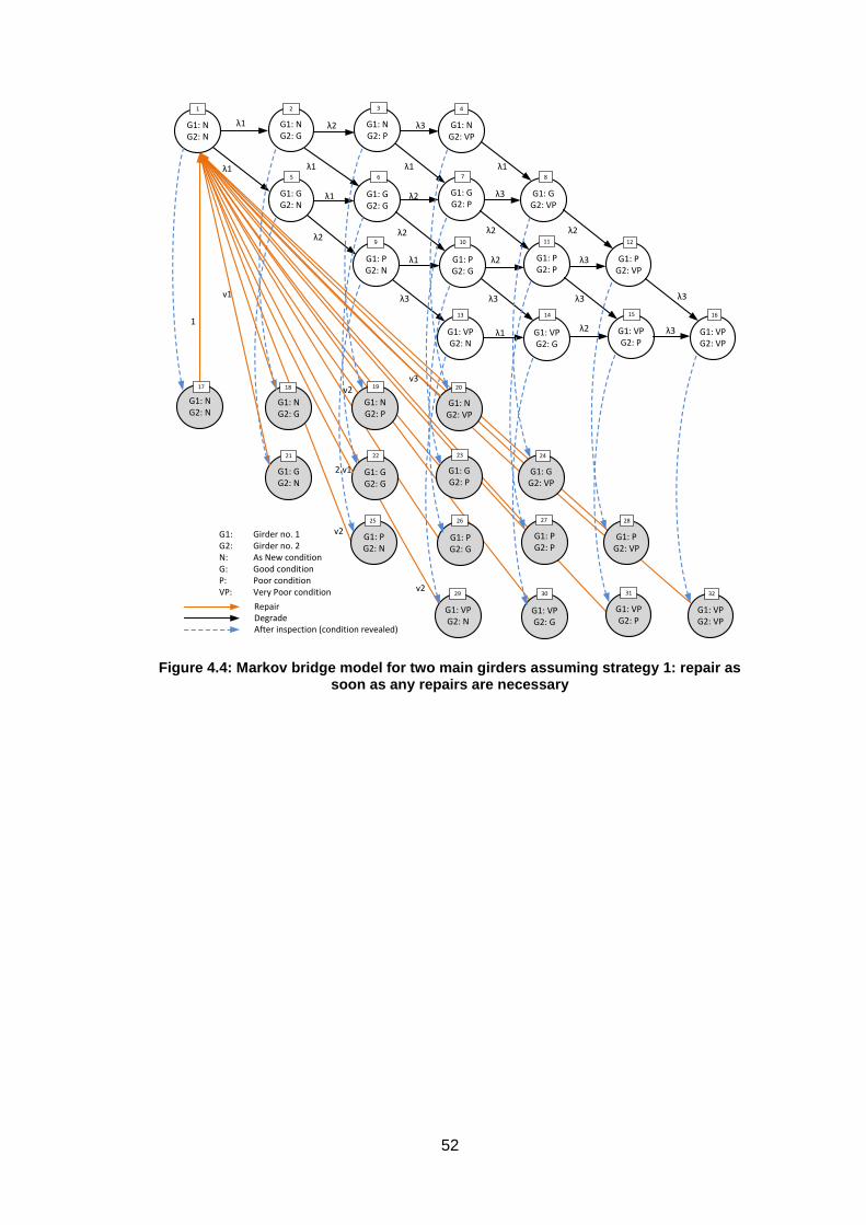
52
Figure 4.4: Markov bridge model for two main girders assuming strategy 1: repair as soon as any repairs are necessary
G1: NG2: N
G1: NG2: G
G1: NG2: P
G1: NG2: VP
G1: GG2: N
G1: GG2: G
G1: GG2: P
G1: GG2: VP
G1: PG2: N
G1: PG2: G
G1: PG2: P
G1: PG2: VP
G1: VPG2: N
G1: VPG2: G
G1: VPG2: P
G1: VPG2: VP
λ1
λ1 λ1 λ1 λ1
λ1
λ1
λ1
λ2
λ2
λ2 λ2 λ2
λ2
λ2
λ2
λ3
λ3
λ3
λ3
λ3λ3 λ3 λ3
G1: NG2: G
G1: NG2: P
G1: NG2: VP
G1: GG2: N
G1: GG2: G
G1: GG2: P
G1: GG2: VP
G1: PG2: N
G1: PG2: G
G1: PG2: P
G1: PG2: VP
G1: VPG2: N
G1: VPG2: G
G1: VPG2: P
G1: VPG2: VP
v1
1
v2
2.v1
v2
v3
After inspection (condition revealed)
RepairDegrade
v2
G1: NG2: N
1 42 3
5 86 7
9 1210 11
13 1614 15
17 2018 19
21 2422 23
25 2826 27
29 3230 31
G1: Girder no. 1G2: Girder no. 2N: As New conditionG: Good conditionP: Poor conditionVP: Very Poor condition
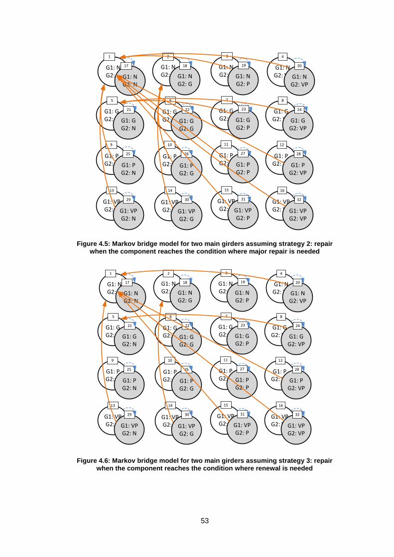
53
Figure 4.5: Markov bridge model for two main girders assuming strategy 2: repair when the component reaches the condition where major repair is needed
Figure 4.6: Markov bridge model for two main girders assuming strategy 3: repair when the component reaches the condition where renewal is needed
G1: NG2: N
G1: NG2: G
G1: NG2: P
G1: NG2: VP
1 42 3
G1: GG2: N
G1: GG2: G
G1: GG2: P
G1: GG2: VP
5 86 7
G1: PG2: N
G1: PG2: G
G1: PG2: P
G1: PG2: VP
9 1210 11
G1: VPG2: N
G1: VPG2: G
G1: VPG2: P
G1: VPG2: VP
13 1614 15
G1: NG2: N
G1: NG2: G
G1: NG2: P
G1: NG2: VP
17 2018 19
G1: GG2: N
G1: GG2: G
G1: GG2: P
G1: GG2: VP
21 2422 23
G1: PG2: N
G1: PG2: G
G1: PG2: P
G1: PG2: VP
25 2826 27
G1: VPG2: N
G1: VPG2: G
G1: VPG2: P
G1: VPG2: VP
29 3230 31
G1: NG2: N
G1: NG2: G
G1: NG2: P
G1: NG2: VP
1 42 3
G1: GG2: N
G1: GG2: G
G1: GG2: P
G1: GG2: VP
5 86 7
G1: PG2: N
G1: PG2: G
G1: PG2: P
G1: PG2: VP
9 1210 11
G1: VPG2: N
G1: VPG2: G
G1: VPG2: P
G1: VPG2: VP
13 1614 15
G1: NG2: N
G1: NG2: G
G1: NG2: P
G1: NG2: VP
17 2018 19
G1: GG2: N
G1: GG2: G
G1: GG2: P
G1: GG2: VP
21 2422 23
G1: PG2: N
G1: PG2: G
G1: PG2: P
G1: PG2: VP
25 2826 27
G1: VPG2: N
G1: VPG2: G
G1: VPG2: P
G1: VPG2: VP
29 3230 31

54
4.2.3 Opportunistic maintenance
Generally, there are a couple of advantages (Samhouri, 2009) for
applying opportunistic maintenance: 1) to extend equipment
lifetime or at least the mean time to the next failure whose repair
may be costly. It is expected that this maintenance policy can
reduce the frequency of service interruption and the many
undesirable consequences of such interruption, and 2) to take
advantage of the resources, efforts and time already dedicated to
the maintenance of other parts in the system in order to cut cost.
Since the bridge model consists of many different elements, the
conditions and deterioration rates of these elements are different
hence the times when interventions are required are also
different. If a component is being repaired, opportunistic
maintenance considers carrying out repair on other components
which have a deteriorated condition but would not normally
instigate maintenance. This takes advantage of any possession
time or preparation required by the major maintenance task to
minimise longer term service disruption. Figure 4.7 shows again
the model for two main girders with maintenance strategy 2 and
identifies the states where opportunistic repair are possible. In
particular, state 23 in the model represents the case that after an
inspection the main girder 1 is discovered to be in a good
condition and the main girder 2 is in a poor condition. Under
maintenance strategy 2, only the main girder 2 will be repaired,
the repair process will bring the system to state 5 where the main
girder 2 is now in the as new condition whilst the main girder 1
remains in the same condition. It is possible in this case to carry
out opportunistic maintenance on main girder 1, this will bring the
system back to state 1 where both component conditions are
restored to the ‘as good as new’ condition. The repair process
represented by an arrow connecting State 23 and State 5 will be
replaced by an arrow from State 23 to State 1. Similarly, Figure
4.8 shows the Markov state diagram for opportunistic repair with
maintenance strategy 3. Again the process of generating the
repair transitions for opportunistic maintenance is carried out
automatically by the software.
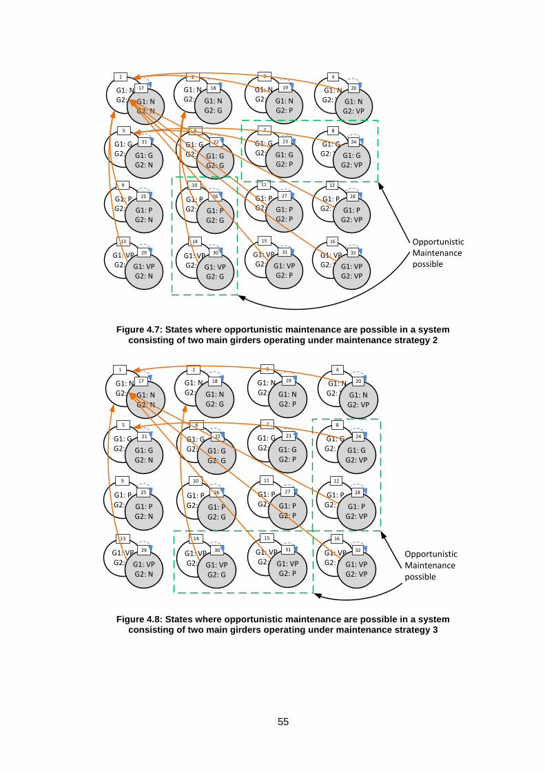
55
Figure 4.7: States where opportunistic maintenance are possible in a system consisting of two main girders operating under maintenance strategy 2
Figure 4.8: States where opportunistic maintenance are possible in a system consisting of two main girders operating under maintenance strategy 3
G1: NG2: N
G1: NG2: G
G1: NG2: P
G1: NG2: VP
1 42 3
G1: GG2: N
G1: GG2: G
G1: GG2: P
G1: GG2: VP
5 86 7
G1: PG2: N
G1: PG2: G
G1: PG2: P
G1: PG2: VP
9 1210 11
G1: VPG2: N
G1: VPG2: G
G1: VPG2: P
G1: VPG2: VP
13 1614 15
G1: NG2: N
G1: NG2: G
G1: NG2: P
G1: NG2: VP
17 2018 19
G1: GG2: N
G1: GG2: G
G1: GG2: P
G1: GG2: VP
21 2422 23
G1: PG2: N
G1: PG2: G
G1: PG2: P
G1: PG2: VP
25 2826 27
G1: VPG2: N
G1: VPG2: G
G1: VPG2: P
G1: VPG2: VP
29 3230 31
Opportunistic Maintenance possible
G1: NG2: N
G1: NG2: G
G1: NG2: P
G1: NG2: VP
1 42 3
G1: GG2: N
G1: GG2: G
G1: GG2: P
G1: GG2: VP
5 86 7
G1: PG2: N
G1: PG2: G
G1: PG2: P
G1: PG2: VP
9 1210 11
G1: VPG2: N
G1: VPG2: G
G1: VPG2: P
G1: VPG2: VP
13 1614 15
G1: NG2: N
G1: NG2: G
G1: NG2: P
G1: NG2: VP
17 2018 19
G1: GG2: N
G1: GG2: G
G1: GG2: P
G1: GG2: VP
21 2422 23
G1: PG2: N
G1: PG2: G
G1: PG2: P
G1: PG2: VP
25 2826 27
G1: VPG2: N
G1: VPG2: G
G1: VPG2: P
G1: VPG2: VP
29 3230 31Opportunistic Maintenance possible
56
4.2.4 Environment factor
Depending on the environment where the bridge components
operate, the degradation rate will be different. There are three
types of environment generally considered by the industry
(Network Rail, 2010a), and their definitions are as followed:
Aggressive: exposed to marine environments or harsh
environments with repeat cycles of freezing and thawing,
wetting and drying.
Moderate: all bridges which do not fall into either of the
two other categories.
Benign: situated in a windy, non-marine, non-road
environment which dries bridge without salt deposition.
Each type of structure in those environments would have different
deterioration rates, therefore the deterioration rates should be
adjusted accordingly with an adjustment factor. There was no
study in the literature that quantifies the effects however, the
experts opinion (Network Rail, 2010a) is that, for all types of
structure, the component deteriorates three times faster in an
aggressive environment compared with the benign environment;
and the degradation rate is 30% less in a moderate environment
compared with an aggressive environment. The estimated effects
of environment on the deterioration rates of different materials
are presented in a table given in Appendix B. Once the
environment is specified in the model, the deterioration rate is
adjusted by multiplying by the appropriate adjustment factor, this
allows the model to effectively consider the effect of different
deterioration rates.
4.2.5 Servicing frequency
Another factor that changes the degradation rate is the servicing
frequency. Servicing work does not change the state of the
component but helps slow down the deterioration rate and
increases the time until the next intervention is needed. Servicing
work includes: painting, pigeon proofing, cleaning debris. A
simple study was carried out in the previous chapter, to
determine the effects of servicing frequency on the deterioration
rates by comparing the degradation rates of the same group of
components that have a different servicing frequency recorded. A
linear relationship was established to model this effect. Therefore,
at a given servicing interval, the deterioration rate of a particular
57
element is adjusted accordingly. The adjustment factors were
discussed and presented in Chapter 3 - 3.6.2. The model is then
capable of capturing and modelling the effects that a different
servicing interval will have on the degradation process of bridge
elements.
4.2.6 Transition rates
4.2.6.1 Degradation rates
The deterioration rates are attained by examining the database
and maintenance records and analysing the times that each
element takes to deteriorate to the point where a certain type of
maintenance is required. These rates are obtained in Chapter 3 -
3.6.1, however they govern the process from the ‘as new’ state.
The Markov model needs the transition rates between two
adjacent states (good to poor, poor to very poor). The rate from
state i to state j can be calculated as the inverse of the mean
time reaching state j from state i, MTTFi,j this can be estimated
from:
(4.1)
Giving:
(4.2)
is the deterioration rate from state i to state j and is calculated
as the inverse of MTTFi,j. is the deterioration rate from the new
state to state i. MTTF1,i and MTTF1,j are taken as the mean values
of the distributions obtained in Chapter 3 - 3.6.1. It is important
to know that those distributions are Weibull distributions however
the Markov model only allows constant transition rates i.e.
exponential distribution to be modelled, therefore the mean
values of the Weibull distributions obtained were used to estimate
the transition rates of Markov bridge model. This is assumed good
estimations since the β values obtained for those Weibull
distributions are very close to 1 (Chapter 3 - 3.6.1).
As mentioned previously, the degradation rate is affected by the
environment and servicing frequency, thus the final step of
deducing the degradation rate is by adjustment according to
Equation (4.3).
58
(4.3)
where
is the adjustment factor according to different
environment as given in Appendix B
is the adjustment factor according to different
servicing frequency as given in Chapter 3 -3.6.2
4.2.6.2 Repair rates
The repair rates, , , are included in the model as illustrated
in Figure 4.3, representing the rates that bring the component
from the good, poor, and very poor state back to the ‘as new’
state. The time to repair consists of two main components:
the time to schedule the repair (TS)
the time of the actual repair work being carried out (TR)
The time of repair is calculated as the duration of the repair
carried out. The distribution of these repair times were obtained
in Chapter 3 - 3.6.3. Again, the mean values of these
distributions were used as the values of TR.
The time to schedule the work is defined as the duration between
when the work was identified as being necessary and when the
work actually starts. TS is essentially a parameter in the model
that dictates the delay of any repair works.
Thus the repair rate can be calculated as:
(4.4)
4.2.6.3 Transition rate matrix
There are two phases in the model:
The first phase is the continuous phase between any two
inspections, the system equation is governed by equation (4.5)
where Q is the matrix representing the probabilities of being in
each state; A is the transition rate matrix based on the
deterioration rates and repair rates as given in Equation (4.5);
and is the rate of change of probabilities at each state in the
model. Note that the transition rate matrix given in Equation (4.6)
is for a single bridge element. The transition rate matrix for a
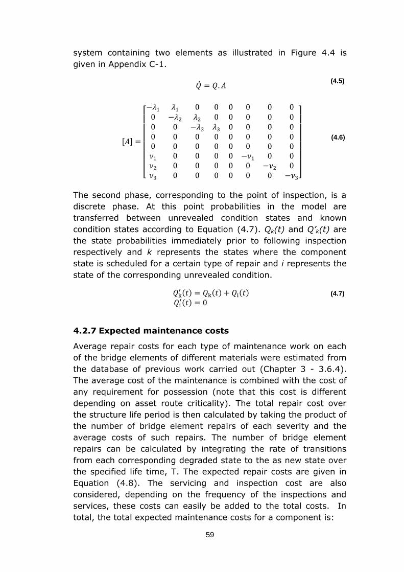
59
system containing two elements as illustrated in Figure 4.4 is
given in Appendix C-1.
(4.5)
[ ]
(4.6)
The second phase, corresponding to the point of inspection, is a
discrete phase. At this point probabilities in the model are
transferred between unrevealed condition states and known
condition states according to Equation (4.7). Qk(t) and Q’k(t) are
the state probabilities immediately prior to following inspection
respectively and k represents the states where the component
state is scheduled for a certain type of repair and i represents the
state of the corresponding unrevealed condition.
( ) ( ) ( )
( )
(4.7)
4.2.7 Expected maintenance costs
Average repair costs for each type of maintenance work on each
of the bridge elements of different materials were estimated from
the database of previous work carried out (Chapter 3 - 3.6.4).
The average cost of the maintenance is combined with the cost of
any requirement for possession (note that this cost is different
depending on asset route criticality). The total repair cost over
the structure life period is then calculated by taking the product of
the number of bridge element repairs of each severity and the
average costs of such repairs. The number of bridge element
repairs can be calculated by integrating the rate of transitions
from each corresponding degraded state to the as new state over
the specified life time, T. The expected repair costs are given in
Equation (4.8). The servicing and inspection cost are also
considered, depending on the frequency of the inspections and
services, these costs can easily be added to the total costs. In
total, the total expected maintenance costs for a component is:
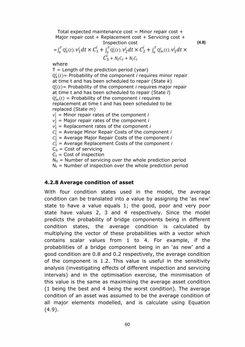
60
Total expected maintenance cost = Minor repair cost + Major repair cost + Replacement cost + Servicing cost +
Inspection cost
=∫ ( )
∫
( )
∫ ( )
(4.8)
where T = Length of the prediction period (year)
( )= Probability of the component i requires minor repair
at time t and has been scheduled to repair (State k)
( )= Probability of the component i requires major repair
at time t and has been scheduled to repair (State l)
( ) = Probability of the component i requires
replacement at time t and has been scheduled to be
replaced (State m)
= Minor repair rates of the component i
= Major repair rates of the component i
= Replacement rates of the component i
= Average Minor Repair Costs of the component i
= Average Major Repair Costs of the component i
= Average Replacement Costs of the component i
CS = Cost of servicing CI = Cost of inspection NS = Number of servicing over the whole prediction period NI = Number of inspection over the whole prediction period
4.2.8 Average condition of asset
With four condition states used in the model, the average
condition can be translated into a value by assigning the ‘as new’
state to have a value equals 1; the good, poor and very poor
state have values 2, 3 and 4 respectively. Since the model
predicts the probability of bridge components being in different
condition states, the average condition is calculated by
multiplying the vector of these probabilities with a vector which
contains scalar values from 1 to 4. For example, if the
probabilities of a bridge component being in an ‘as new’ and a
good condition are 0.8 and 0.2 respectively, the average condition
of the component is 1.2. This value is useful in the sensitivity
analysis (investigating effects of different inspection and servicing
intervals) and in the optimisation exercise, the minimisation of
this value is the same as maximising the average asset condition
(1 being the best and 4 being the worst condition). The average
condition of an asset was assumed to be the average condition of
all major elements modelled, and is calculate using Equation
(4.9).
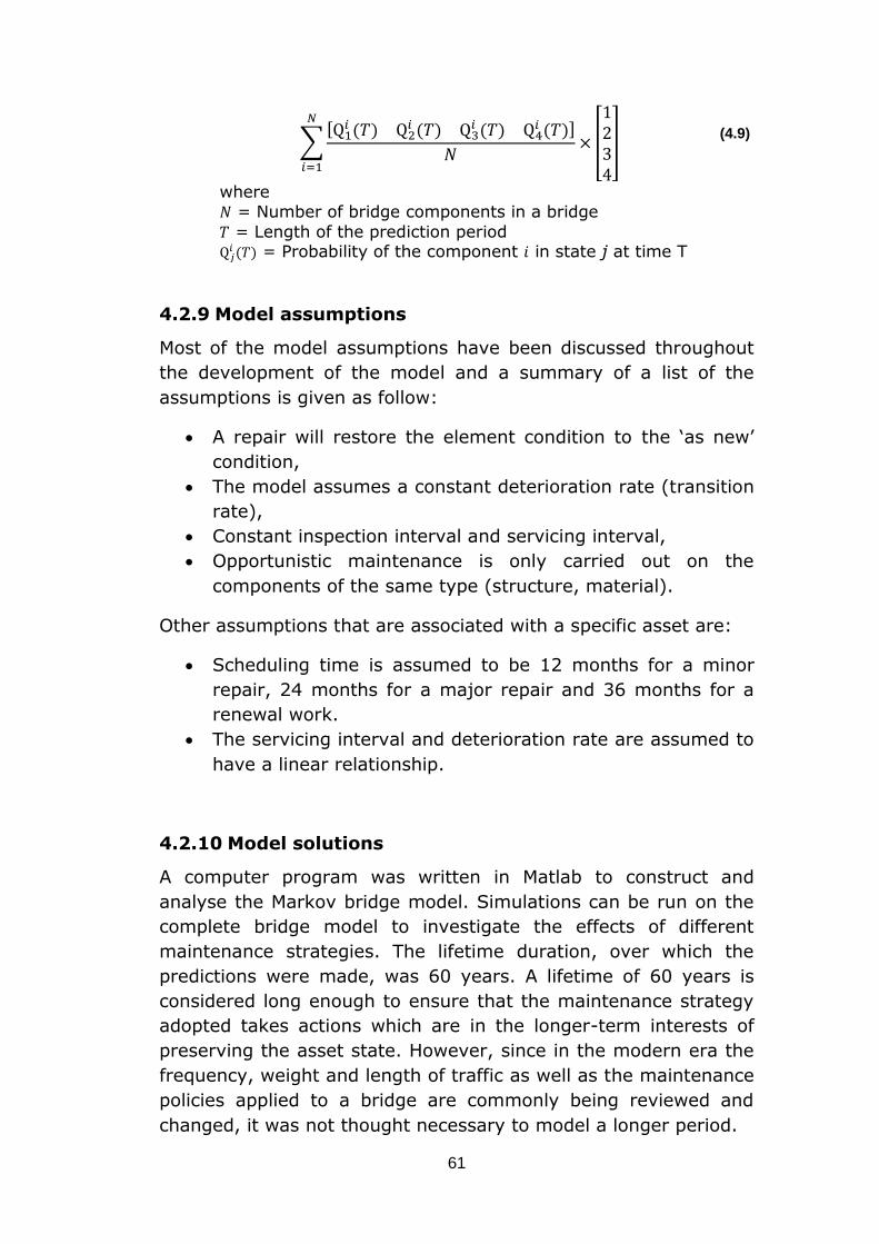
61
∑
( ) ( )
( ) ( )
[
] (4.9)
where
= Number of bridge components in a bridge
= Length of the prediction period
( ) = Probability of the component in state j at time T
4.2.9 Model assumptions
Most of the model assumptions have been discussed throughout
the development of the model and a summary of a list of the
assumptions is given as follow:
A repair will restore the element condition to the ‘as new’
condition,
The model assumes a constant deterioration rate (transition
rate),
Constant inspection interval and servicing interval,
Opportunistic maintenance is only carried out on the
components of the same type (structure, material).
Other assumptions that are associated with a specific asset are:
Scheduling time is assumed to be 12 months for a minor
repair, 24 months for a major repair and 36 months for a
renewal work.
The servicing interval and deterioration rate are assumed to
have a linear relationship.
4.2.10 Model solutions
A computer program was written in Matlab to construct and
analyse the Markov bridge model. Simulations can be run on the
complete bridge model to investigate the effects of different
maintenance strategies. The lifetime duration, over which the
predictions were made, was 60 years. A lifetime of 60 years is
considered long enough to ensure that the maintenance strategy
adopted takes actions which are in the longer-term interests of
preserving the asset state. However, since in the modern era the
frequency, weight and length of traffic as well as the maintenance
policies applied to a bridge are commonly being reviewed and
changed, it was not thought necessary to model a longer period.
62
The transitions in the model are represented by rates. The
inspection transitions were modelled as instantaneous shifts in
probability at discrete times. These rates form a system of
differential equations that was solved by a 4th order Runge-Kutta
method with variable time step to speed up the process. The step
size decides the accuracy of the model solutions. The step size
must be small enough that a two-state-jump does not occur
within the given time step. Given the slow degradation rate of the
bridge assets, it is believed that a 0.01 year (7 days) time step is
reasonably small enough. Therefore the initial time step is
assumed to be 0.01 year and the average step size over the
whole solution routine was 0.03 years. The integration procedure
gives the probability of the bridge component being in the
different states and the probability of being in a particular
condition can be found by adding the probabilities of the being all
in all the states that represent that condition. A 2,048 Markov
state model was generated in this study and the computation
time was about 1 minute.
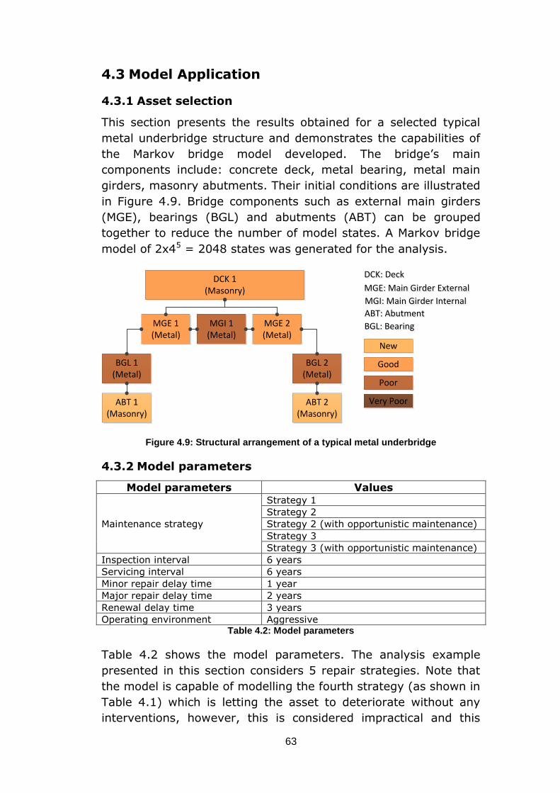
63
4.3 Model Application
4.3.1 Asset selection
This section presents the results obtained for a selected typical
metal underbridge structure and demonstrates the capabilities of
the Markov bridge model developed. The bridge’s main
components include: concrete deck, metal bearing, metal main
girders, masonry abutments. Their initial conditions are illustrated
in Figure 4.9. Bridge components such as external main girders
(MGE), bearings (BGL) and abutments (ABT) can be grouped
together to reduce the number of model states. A Markov bridge
model of 2x45 = 2048 states was generated for the analysis.
Figure 4.9: Structural arrangement of a typical metal underbridge
4.3.2 Model parameters
Model parameters Values
Maintenance strategy
Strategy 1
Strategy 2
Strategy 2 (with opportunistic maintenance)
Strategy 3
Strategy 3 (with opportunistic maintenance)
Inspection interval 6 years
Servicing interval 6 years
Minor repair delay time 1 year
Major repair delay time 2 years
Renewal delay time 3 years
Operating environment Aggressive Table 4.2: Model parameters
Table 4.2 shows the model parameters. The analysis example
presented in this section considers 5 repair strategies. Note that
the model is capable of modelling the fourth strategy (as shown in
Table 4.1) which is letting the asset to deteriorate without any
interventions, however, this is considered impractical and this
DCK 1(Masonry)
MGE 1(Metal)
MGE 2(Metal)
BGL 1(Metal)
BGL 2(Metal)
ABT 1(Masonry)
ABT 2(Masonry)
Good
New
Poor
Very Poor
MGI 1(Metal)
DCK: DeckDCK: Deck
MGE: Main Girder External MGE: Main Girder External
MGI: Main Girder Internal MGI: Main Girder Internal
ABT: AbutmentABT: Abutment
BGL: BearingBGL: Bearing
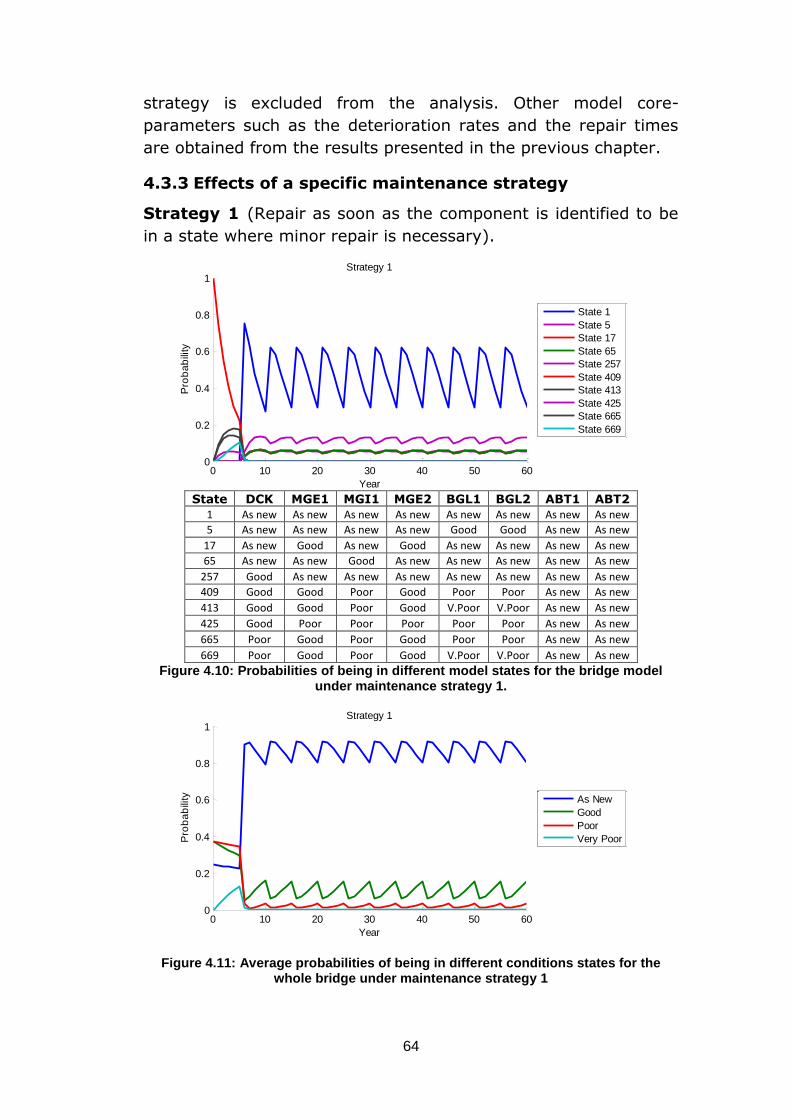
64
strategy is excluded from the analysis. Other model core-
parameters such as the deterioration rates and the repair times
are obtained from the results presented in the previous chapter.
4.3.3 Effects of a specific maintenance strategy
Strategy 1 (Repair as soon as the component is identified to be
in a state where minor repair is necessary).
State DCK MGE1 MGI1 MGE2 BGL1 BGL2 ABT1 ABT2
1 As new As new As new As new As new As new As new As new
5 As new As new As new As new Good Good As new As new
17 As new Good As new Good As new As new As new As new
65 As new As new Good As new As new As new As new As new
257 Good As new As new As new As new As new As new As new
409 Good Good Poor Good Poor Poor As new As new
413 Good Good Poor Good V.Poor V.Poor As new As new
425 Good Poor Poor Poor Poor Poor As new As new
665 Poor Good Poor Good Poor Poor As new As new
669 Poor Good Poor Good V.Poor V.Poor As new As new
Figure 4.10: Probabilities of being in different model states for the bridge model under maintenance strategy 1.
Figure 4.11: Average probabilities of being in different conditions states for the whole bridge under maintenance strategy 1
0 10 20 30 40 50 600
0.2
0.4
0.6
0.8
1
Year
Pro
ba
bili
ty
Strategy 1
State 1
State 5
State 17
State 65
State 257
State 409
State 413
State 425
State 665
State 669
0 10 20 30 40 50 600
0.2
0.4
0.6
0.8
1
Year
Pro
ba
bili
ty
Strategy 1
As New
Good
Poor
Very Poor
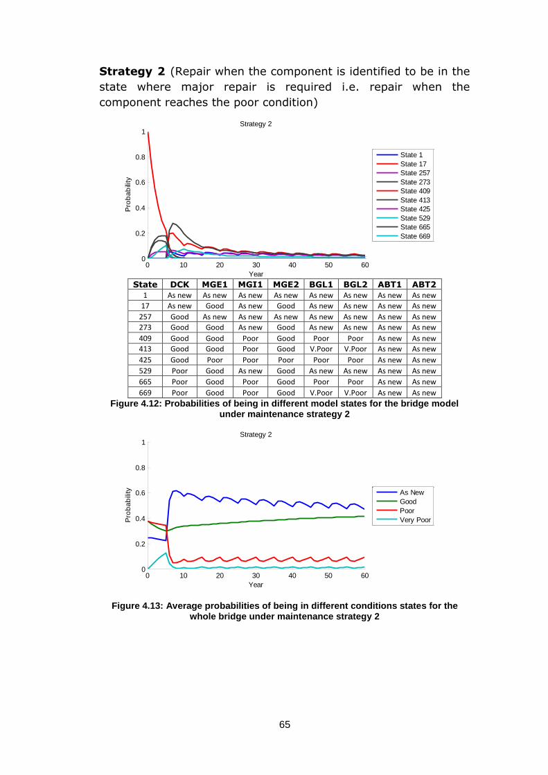
65
Strategy 2 (Repair when the component is identified to be in the
state where major repair is required i.e. repair when the
component reaches the poor condition)
State DCK MGE1 MGI1 MGE2 BGL1 BGL2 ABT1 ABT2
1 As new As new As new As new As new As new As new As new
17 As new Good As new Good As new As new As new As new
257 Good As new As new As new As new As new As new As new
273 Good Good As new Good As new As new As new As new
409 Good Good Poor Good Poor Poor As new As new
413 Good Good Poor Good V.Poor V.Poor As new As new
425 Good Poor Poor Poor Poor Poor As new As new
529 Poor Good As new Good As new As new As new As new
665 Poor Good Poor Good Poor Poor As new As new
669 Poor Good Poor Good V.Poor V.Poor As new As new
Figure 4.12: Probabilities of being in different model states for the bridge model under maintenance strategy 2
Figure 4.13: Average probabilities of being in different conditions states for the whole bridge under maintenance strategy 2
0 10 20 30 40 50 600
0.2
0.4
0.6
0.8
1
Year
Pro
ba
bili
tyStrategy 2
State 1
State 17
State 257
State 273
State 409
State 413
State 425
State 529
State 665
State 669
0 10 20 30 40 50 600
0.2
0.4
0.6
0.8
1
Year
Pro
ba
bili
ty
Strategy 2
As New
Good
Poor
Very Poor
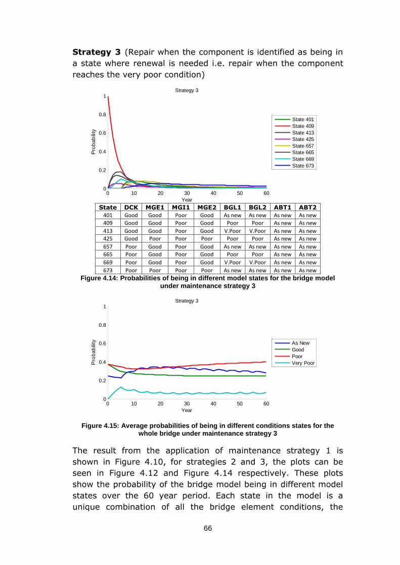
66
Strategy 3 (Repair when the component is identified as being in
a state where renewal is needed i.e. repair when the component
reaches the very poor condition)
State DCK MGE1 MGI1 MGE2 BGL1 BGL2 ABT1 ABT2
401 Good Good Poor Good As new As new As new As new
409 Good Good Poor Good Poor Poor As new As new
413 Good Good Poor Good V.Poor V.Poor As new As new
425 Good Poor Poor Poor Poor Poor As new As new
657 Poor Good Poor Good As new As new As new As new
665 Poor Good Poor Good Poor Poor As new As new
669 Poor Good Poor Good V.Poor V.Poor As new As new
673 Poor Poor Poor Poor As new As new As new As new
Figure 4.14: Probabilities of being in different model states for the bridge model under maintenance strategy 3
Figure 4.15: Average probabilities of being in different conditions states for the whole bridge under maintenance strategy 3
The result from the application of maintenance strategy 1 is
shown in Figure 4.10, for strategies 2 and 3, the plots can be
seen in Figure 4.12 and Figure 4.14 respectively. These plots
show the probability of the bridge model being in different model
states over the 60 year period. Each state in the model is a
unique combination of all the bridge element conditions, the
0 10 20 30 40 50 600
0.2
0.4
0.6
0.8
1
Year
Pro
ba
bili
tyStrategy 3
State 401
State 409
State 413
State 425
State 657
State 665
State 669
State 673
0 10 20 30 40 50 600
0.2
0.4
0.6
0.8
1
Year
Pro
ba
bili
ty
Strategy 3
As New
Good
Poor
Very Poor
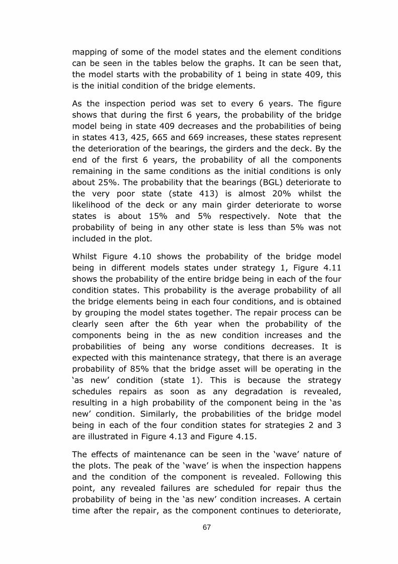
67
mapping of some of the model states and the element conditions
can be seen in the tables below the graphs. It can be seen that,
the model starts with the probability of 1 being in state 409, this
is the initial condition of the bridge elements.
As the inspection period was set to every 6 years. The figure
shows that during the first 6 years, the probability of the bridge
model being in state 409 decreases and the probabilities of being
in states 413, 425, 665 and 669 increases, these states represent
the deterioration of the bearings, the girders and the deck. By the
end of the first 6 years, the probability of all the components
remaining in the same conditions as the initial conditions is only
about 25%. The probability that the bearings (BGL) deteriorate to
the very poor state (state 413) is almost 20% whilst the
likelihood of the deck or any main girder deteriorate to worse
states is about 15% and 5% respectively. Note that the
probability of being in any other state is less than 5% was not
included in the plot.
Whilst Figure 4.10 shows the probability of the bridge model
being in different models states under strategy 1, Figure 4.11
shows the probability of the entire bridge being in each of the four
condition states. This probability is the average probability of all
the bridge elements being in each four conditions, and is obtained
by grouping the model states together. The repair process can be
clearly seen after the 6th year when the probability of the
components being in the as new condition increases and the
probabilities of being any worse conditions decreases. It is
expected with this maintenance strategy, that there is an average
probability of 85% that the bridge asset will be operating in the
‘as new’ condition (state 1). This is because the strategy
schedules repairs as soon as any degradation is revealed,
resulting in a high probability of the component being in the ‘as
new’ condition. Similarly, the probabilities of the bridge model
being in each of the four condition states for strategies 2 and 3
are illustrated in Figure 4.13 and Figure 4.15.
The effects of maintenance can be seen in the ‘wave’ nature of
the plots. The peak of the ‘wave’ is when the inspection happens
and the condition of the component is revealed. Following this
point, any revealed failures are scheduled for repair thus the
probability of being in the ‘as new’ condition increases. A certain
time after the repair, as the component continues to deteriorate,
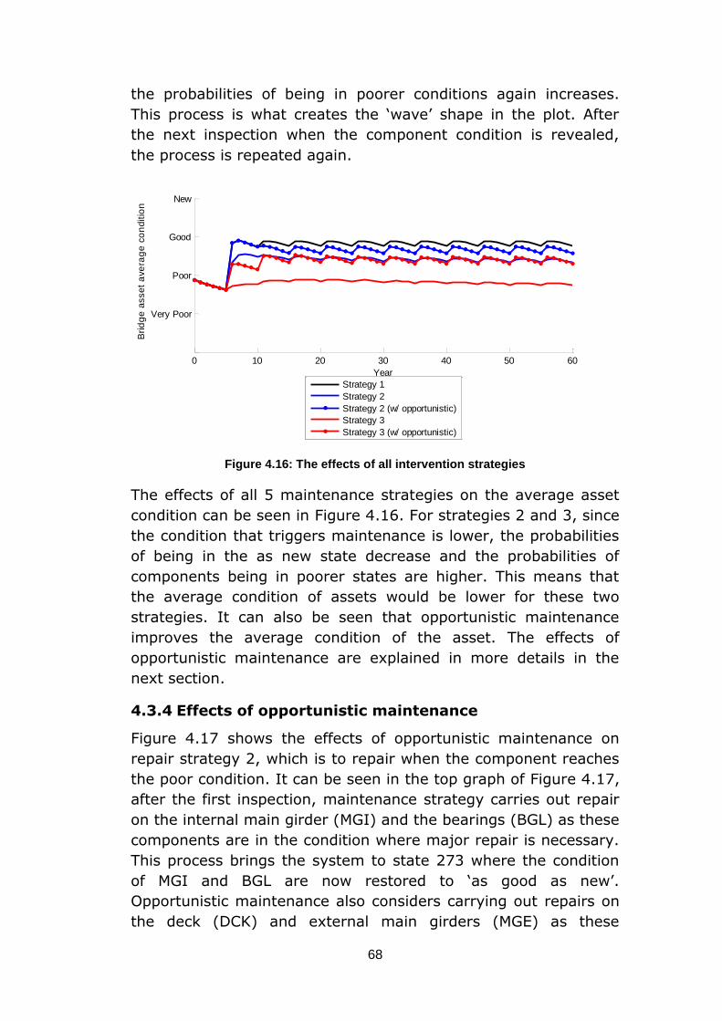
68
the probabilities of being in poorer conditions again increases.
This process is what creates the ‘wave’ shape in the plot. After
the next inspection when the component condition is revealed,
the process is repeated again.
Figure 4.16: The effects of all intervention strategies
The effects of all 5 maintenance strategies on the average asset
condition can be seen in Figure 4.16. For strategies 2 and 3, since
the condition that triggers maintenance is lower, the probabilities
of being in the as new state decrease and the probabilities of
components being in poorer states are higher. This means that
the average condition of assets would be lower for these two
strategies. It can also be seen that opportunistic maintenance
improves the average condition of the asset. The effects of
opportunistic maintenance are explained in more details in the
next section.
4.3.4 Effects of opportunistic maintenance
Figure 4.17 shows the effects of opportunistic maintenance on
repair strategy 2, which is to repair when the component reaches
the poor condition. It can be seen in the top graph of Figure 4.17,
after the first inspection, maintenance strategy carries out repair
on the internal main girder (MGI) and the bearings (BGL) as these
components are in the condition where major repair is necessary.
This process brings the system to state 273 where the condition
of MGI and BGL are now restored to ‘as good as new’.
Opportunistic maintenance also considers carrying out repairs on
the deck (DCK) and external main girders (MGE) as these
0 10 20 30 40 50 60
Very Poor
Poor
Good
New
Year
Bri
dg
e a
sse
t a
ve
rag
e c
on
ditio
n
Strategy 1
Strategy 2
Strategy 2 (w/ opportunistic)
Strategy 3
Strategy 3 (w/ opportunistic)

69
components have not yet reached the point where the repair is
triggered for this maintenance strategy however they are in the
state where repair is possible. This means that in this case all the
components are being scheduled for repair at the same time, and
all the components are expected to be in the ‘as good as new’
condition after the first repair, this is reflected in the bottom
graph of Figure 4.17 as the probability of the model of being in
state 1 increases to almost 80% after the first inspection.
As the result of applying opportunistic maintenance, it is more
likely that the components will be operating in better conditions
when compared with the case where opportunistic maintenance is
not employed, the expected number of repairs will also increase
resulting in higher maintenance costs at the start of the bridge
modelling period.
Even though it is clear to see the components are more reliable
when employing opportunistic maintenance, it is not clear how
the whole life-cycle cost is affected. It is expected a high
maintenance cost at the beginning of the lifetime as more repair
needs to be done but since the component condition is improved
early in the lifetime, the expected maintenance cost in the future
is expected to reduce. This effect will be investigated in later
section 4.3.6 when analysing the expected maintenance costs.
The effect of opportunistic maintenance, when applying
maintenance strategy 3, is demonstrated in Figure 4.18. Note
that, for strategy 1, opportunistic maintenance is unnecessary,
this is because any component that reaches the good condition
would be maintained immediately, thus, applying opportunistic
maintenance for this strategy would produce the same results as
illustrated in Figure 4.10.
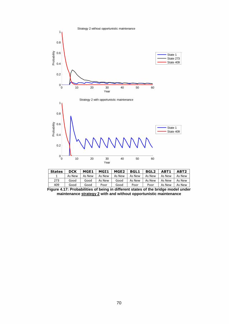
70
States DCK MGE1 MGI1 MGE2 BGL1 BGL2 ABT1 ABT2
1 As New As New As New As New As New As New As New As New
273 Good Good As New Good As New As New As New As New
409 Good Good Poor Good Poor Poor As New As New
Figure 4.17: Probabilities of being in different states of the bridge model under maintenance strategy 2 with and without opportunistic maintenance
0 10 20 30 40 50 600
0.2
0.4
0.6
0.8
1
Year
Pro
ba
bili
ty
Strategy 2 without opportunistic maintenance
State 1
State 273
State 409
0 10 20 30 40 50 600
0.2
0.4
0.6
0.8
1
Year
Pro
ba
bili
ty
Strategy 2 with opportunistic maintenance
State 1
State 409
71
State DCK MGE1 MGI1 MGE2 BGL1 BGL2 ABT1 ABT2
1 As new As new As new As new As new As new As new As new
257 Good As new As new As new As new As new As new As new
401 Good Good Poor Good As new As new As new As new
409 Good Good Poor Good Poor Poor As new As new
413 Good Good Poor Good V.Poor V.Poor As new As new
425 Good Poor Poor Poor Poor Poor As new As new
657 Poor Good Poor Good As new As new As new As new
665 Poor Good Poor Good Poor Poor As new As new
669 Poor Good Poor Good V.Poor V.Poor As new As new
673 Poor Poor Poor Poor As new As new As new As new
Figure 4.18: Probabilities of being in different states of the bridge model under maintenance strategy 3 with and without opportunistic maintenance
4.3.5 Analysis on a single bridge element
As well as predicting the probability of the bridge model being in
different states, analysis can be done on a single component to
investigate the effect that a certain maintenance strategy will
have on a particular component. This information is useful to
identify critical components in the structure as well as supporting
the maintenance decision making process. Figure 4.19 and Figure
4.20 plot the probability distribution for the single elements:
abutment and metal bearing respectively. The plots show that
0 10 20 30 40 50 600
0.2
0.4
0.6
0.8
1
Year
Pro
ba
bili
ty
Strategy 3 without opportunistic maintenance
State 401
State 409
State 413
State 425
State 657
State 665
State 669
State 673
0 10 20 30 40 50 600
0.2
0.4
0.6
0.8
1
Year
Pro
ba
bili
ty
Strategy 3 with opportunistic maintenance
State 1
State 257
State 409
State 413
State 425
State 665
State 669
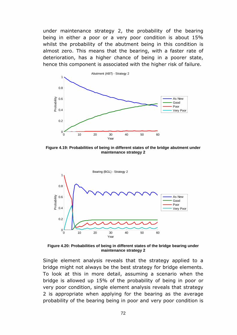
72
under maintenance strategy 2, the probability of the bearing
being in either a poor or a very poor condition is about 15%
whilst the probability of the abutment being in this condition is
almost zero. This means that the bearing, with a faster rate of
deterioration, has a higher chance of being in a poorer state,
hence this component is associated with the higher risk of failure.
Figure 4.19: Probabilities of being in different states of the bridge abutment under maintenance strategy 2
Figure 4.20: Probabilities of being in different states of the bridge bearing under maintenance strategy 2
Single element analysis reveals that the strategy applied to a
bridge might not always be the best strategy for bridge elements.
To look at this in more detail, assuming a scenario when the
bridge is allowed up 15% of the probability of being in poor or
very poor condition, single element analysis reveals that strategy
2 is appropriate when applying for the bearing as the average
probability of the bearing being in poor and very poor condition is
0 10 20 30 40 50 600
0.2
0.4
0.6
0.8
1
Year
Pro
ba
bili
ty
Abutment (ABT) - Strategy 2
As New
Good
Poor
Very Poor
0 10 20 30 40 50 600
0.2
0.4
0.6
0.8
1
Year
Pro
ba
bili
ty
Bearing (BGL) - Strategy 2
As New
Good
Poor
Very Poor
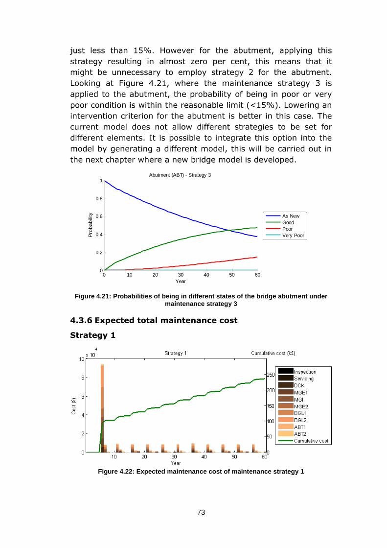
73
just less than 15%. However for the abutment, applying this
strategy resulting in almost zero per cent, this means that it
might be unnecessary to employ strategy 2 for the abutment.
Looking at Figure 4.21, where the maintenance strategy 3 is
applied to the abutment, the probability of being in poor or very
poor condition is within the reasonable limit (<15%). Lowering an
intervention criterion for the abutment is better in this case. The
current model does not allow different strategies to be set for
different elements. It is possible to integrate this option into the
model by generating a different model, this will be carried out in
the next chapter where a new bridge model is developed.
Figure 4.21: Probabilities of being in different states of the bridge abutment under maintenance strategy 3
4.3.6 Expected total maintenance cost
Strategy 1
Figure 4.22: Expected maintenance cost of maintenance strategy 1
0 10 20 30 40 50 600
0.2
0.4
0.6
0.8
1
Year
Pro
ba
bili
ty
Abutment (ABT) - Strategy 3
As New
Good
Poor
Very Poor
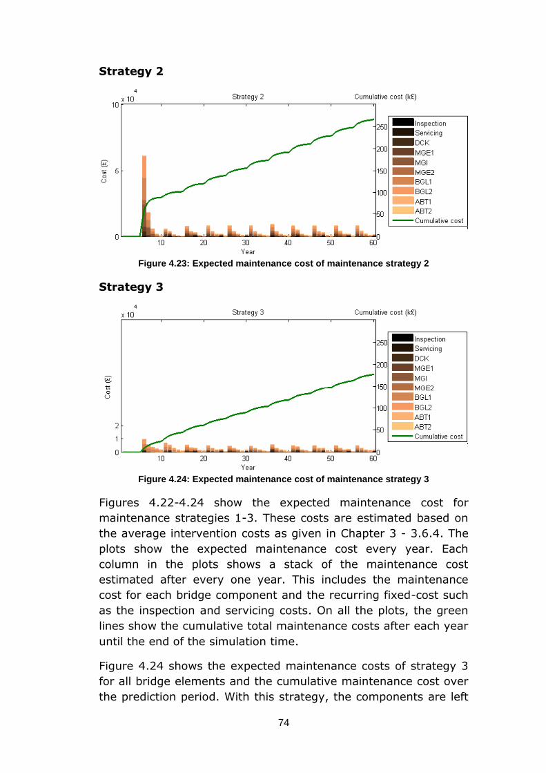
74
Strategy 2
Figure 4.23: Expected maintenance cost of maintenance strategy 2
Strategy 3
Figure 4.24: Expected maintenance cost of maintenance strategy 3
Figures 4.22-4.24 show the expected maintenance cost for
maintenance strategies 1-3. These costs are estimated based on
the average intervention costs as given in Chapter 3 - 3.6.4. The
plots show the expected maintenance cost every year. Each
column in the plots shows a stack of the maintenance cost
estimated after every one year. This includes the maintenance
cost for each bridge component and the recurring fixed-cost such
as the inspection and servicing costs. On all the plots, the green
lines show the cumulative total maintenance costs after each year
until the end of the simulation time.
Figure 4.24 shows the expected maintenance costs of strategy 3
for all bridge elements and the cumulative maintenance cost over
the prediction period. With this strategy, the components are left
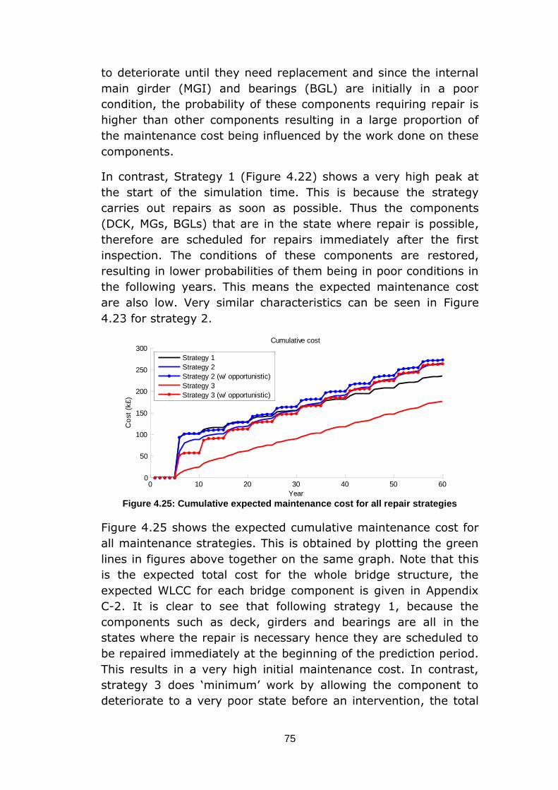
75
to deteriorate until they need replacement and since the internal
main girder (MGI) and bearings (BGL) are initially in a poor
condition, the probability of these components requiring repair is
higher than other components resulting in a large proportion of
the maintenance cost being influenced by the work done on these
components.
In contrast, Strategy 1 (Figure 4.22) shows a very high peak at
the start of the simulation time. This is because the strategy
carries out repairs as soon as possible. Thus the components
(DCK, MGs, BGLs) that are in the state where repair is possible,
therefore are scheduled for repairs immediately after the first
inspection. The conditions of these components are restored,
resulting in lower probabilities of them being in poor conditions in
the following years. This means the expected maintenance cost
are also low. Very similar characteristics can be seen in Figure
4.23 for strategy 2.
Figure 4.25: Cumulative expected maintenance cost for all repair strategies
Figure 4.25 shows the expected cumulative maintenance cost for
all maintenance strategies. This is obtained by plotting the green
lines in figures above together on the same graph. Note that this
is the expected total cost for the whole bridge structure, the
expected WLCC for each bridge component is given in Appendix
C-2. It is clear to see that following strategy 1, because the
components such as deck, girders and bearings are all in the
states where the repair is necessary hence they are scheduled to
be repaired immediately at the beginning of the prediction period.
This results in a very high initial maintenance cost. In contrast,
strategy 3 does ‘minimum’ work by allowing the component to
deteriorate to a very poor state before an intervention, the total
0 10 20 30 40 50 600
50
100
150
200
250
300
Year
Co
st
(k£
)
Cumulative cost
Strategy 1
Strategy 2
Strategy 2 (w/ opportunistic)
Strategy 3
Strategy 3 (w/ opportunistic)
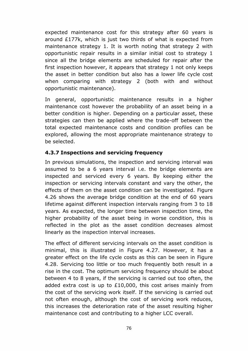
76
expected maintenance cost for this strategy after 60 years is
around £177k, which is just two thirds of what is expected from
maintenance strategy 1. It is worth noting that strategy 2 with
opportunistic repair results in a similar initial cost to strategy 1
since all the bridge elements are scheduled for repair after the
first inspection however, it appears that strategy 1 not only keeps
the asset in better condition but also has a lower life cycle cost
when comparing with strategy 2 (both with and without
opportunistic maintenance).
In general, opportunistic maintenance results in a higher
maintenance cost however the probability of an asset being in a
better condition is higher. Depending on a particular asset, these
strategies can then be applied where the trade-off between the
total expected maintenance costs and condition profiles can be
explored, allowing the most appropriate maintenance strategy to
be selected.
4.3.7 Inspections and servicing frequency
In previous simulations, the inspection and servicing interval was
assumed to be a 6 years interval i.e. the bridge elements are
inspected and serviced every 6 years. By keeping either the
inspection or servicing intervals constant and vary the other, the
effects of them on the asset condition can be investigated. Figure
4.26 shows the average bridge condition at the end of 60 years
lifetime against different inspection intervals ranging from 3 to 18
years. As expected, the longer time between inspection time, the
higher probability of the asset being in worse condition, this is
reflected in the plot as the asset condition decreases almost
linearly as the inspection interval increases.
The effect of different servicing intervals on the asset condition is
minimal, this is illustrated in Figure 4.27. However, it has a
greater effect on the life cycle costs as this can be seen in Figure
4.28. Servicing too little or too much frequently both result in a
rise in the cost. The optimum servicing frequency should be about
between 4 to 8 years, if the servicing is carried out too often, the
added extra cost is up to £10,000, this cost arises mainly from
the cost of the servicing work itself. If the servicing is carried out
not often enough, although the cost of servicing work reduces,
this increases the deterioration rate of the asset resulting higher
maintenance cost and contributing to a higher LCC overall.
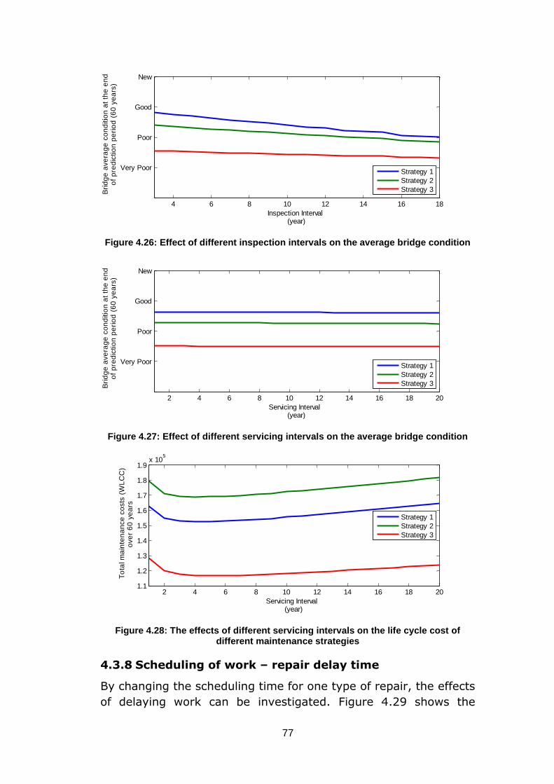
77
Figure 4.26: Effect of different inspection intervals on the average bridge condition
Figure 4.27: Effect of different servicing intervals on the average bridge condition
Figure 4.28: The effects of different servicing intervals on the life cycle cost of different maintenance strategies
4.3.8 Scheduling of work – repair delay time
By changing the scheduling time for one type of repair, the effects
of delaying work can be investigated. Figure 4.29 shows the
4 6 8 10 12 14 16 18
Very Poor
Poor
Good
New
Inspection Interval(year)
Bri
dg
e a
ve
rag
e c
on
ditio
n a
t th
e e
nd
of
pre
dic
tio
n p
eri
od
(6
0 y
ea
rs)
Strategy 1
Strategy 2
Strategy 3
2 4 6 8 10 12 14 16 18 20
Very Poor
Poor
Good
New
Servicing Interval(year)
Bri
dg
e a
ve
rag
e c
on
ditio
n a
t th
e e
nd
of
pre
dic
tio
n p
eri
od
(6
0 y
ea
rs)
Strategy 1
Strategy 2
Strategy 3
2 4 6 8 10 12 14 16 18 201.1
1.2
1.3
1.4
1.5
1.6
1.7
1.8
1.9x 10
5
Servicing Interval(year)
To
tal m
ain
ten
an
ce
co
sts
(W
LC
C)
ove
r 6
0 y
ea
rs
Strategy 1
Strategy 2
Strategy 3
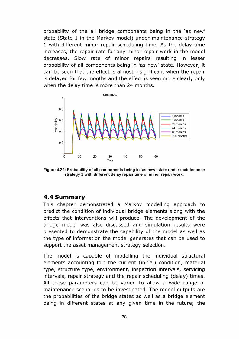
78
probability of the all bridge components being in the ‘as new’
state (State 1 in the Markov model) under maintenance strategy
1 with different minor repair scheduling time. As the delay time
increases, the repair rate for any minor repair work in the model
decreases. Slow rate of minor repairs resulting in lesser
probability of all components being in ‘as new’ state. However, it
can be seen that the effect is almost insignificant when the repair
is delayed for few months and the effect is seen more clearly only
when the delay time is more than 24 months.
Figure 4.29: Probability of all components being in ‘as new’ state under maintenance strategy 1 with different delay repair time of minor repair work.
4.4 Summary
This chapter demonstrated a Markov modelling approach to
predict the condition of individual bridge elements along with the
effects that interventions will produce. The development of the
bridge model was also discussed and simulation results were
presented to demonstrate the capability of the model as well as
the type of information the model generates that can be used to
support the asset management strategy selection.
The model is capable of modelling the individual structural
elements accounting for: the current (initial) condition, material
type, structure type, environment, inspection intervals, servicing
intervals, repair strategy and the repair scheduling (delay) times.
All these parameters can be varied to allow a wide range of
maintenance scenarios to be investigated. The model outputs are
the probabilities of the bridge states as well as a bridge element
being in different states at any given time in the future; the
0 10 20 30 40 50 600
0.2
0.4
0.6
0.8
1
Year
Pro
ba
bili
ty
Strategy 1
1 months
6 months
12 months
24 months
48 months
120 months
79
expected maintenance cost for each type of intervention for each
bridge component; and the total expected maintenance
expenditure – WLCC over the entire prediction period.
The advantages of the model are: the model is easy to construct
and fast to run the analysis, making it easy to investigate the
effect of different strategies; the model uses the degradation
rates based on real historical work done data that was studied in
the previous chapter; and the model is considered more detailed
than previous bridge models in the literature when accounting for
many factors that influence the degradation and maintenance
processes.
However, it was found that in order to satisfy the requirement of
the Markov modelling technique, the deterioration rates of bridge
components were assumed to be constant. Furthermore, the
model size increases exponentially with the number of the
components making the generation, especially when generating
model for repair strategy, and analysing of the model a time
consuming task for model consists of more components. In the
next chapter, a new bridge model is developed using a novel
modelling technique that offers improvements to the Markov
model as presented in this chapter.

80

81
Chapter 5 - Petri Net Bridge Model
5.1 Introduction
The Petri Net (PN) was developed in 1962 by C. A. Petri (Petri,
1963). This method is increasingly being used to model dynamic
systems in many engineering, science and business fields due to
its flexibility (Girault and Valk, 2002). This technique has not
been applied to bridge modelling before and in this chapter, the
method will be explained, the development of the model and its
key features will also be discussed. The advantages it can offer
over the Markov approach will be illustrated. The chapter first
discusses the original PN method and its development over recent
years as it has been used in a wide range of reliability modelling
problems. The chapter will then describe the components of the
PN used in this project. A number of refinements to the traditional
PN concept, to accommodate the requirement for modelling
railway bridge asset management, are also explained in detail.
Finally, the simulation results are presented.
5.1.1 Original Petri Nets
The original concept of a PN (Schneeweiss, 1999) is a directed
graph with two types of nodes, called places and transitions, they
are linked by arcs. A place represents a particular state or
condition of a system. A token resides in a place to indicate the
state of the system. A transition enables the token to move from
one place to another, this models the changing state of the
system. The dynamic behaviour of the system is modelled in the
PN by the process of the token moving between states.
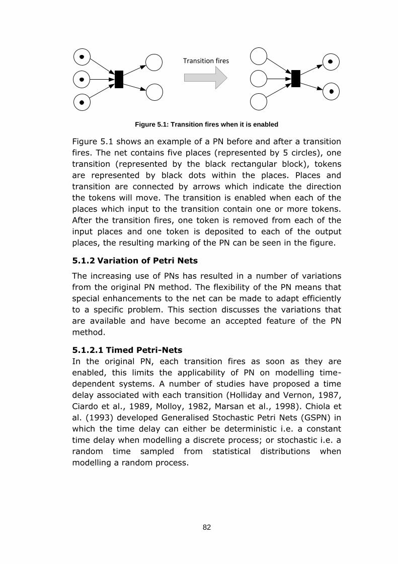
82
Figure 5.1: Transition fires when it is enabled
Figure 5.1 shows an example of a PN before and after a transition
fires. The net contains five places (represented by 5 circles), one
transition (represented by the black rectangular block), tokens
are represented by black dots within the places. Places and
transition are connected by arrows which indicate the direction
the tokens will move. The transition is enabled when each of the
places which input to the transition contain one or more tokens.
After the transition fires, one token is removed from each of the
input places and one token is deposited to each of the output
places, the resulting marking of the PN can be seen in the figure.
5.1.2 Variation of Petri Nets
The increasing use of PNs has resulted in a number of variations
from the original PN method. The flexibility of the PN means that
special enhancements to the net can be made to adapt efficiently
to a specific problem. This section discusses the variations that
are available and have become an accepted feature of the PN
method.
5.1.2.1 Timed Petri-Nets
In the original PN, each transition fires as soon as they are
enabled, this limits the applicability of PN on modelling time-
dependent systems. A number of studies have proposed a time
delay associated with each transition (Holliday and Vernon, 1987,
Ciardo et al., 1989, Molloy, 1982, Marsan et al., 1998). Chiola et
al. (1993) developed Generalised Stochastic Petri Nets (GSPN) in
which the time delay can either be deterministic i.e. a constant
time delay when modelling a discrete process; or stochastic i.e. a
random time sampled from statistical distributions when
modelling a random process.
Transition fires
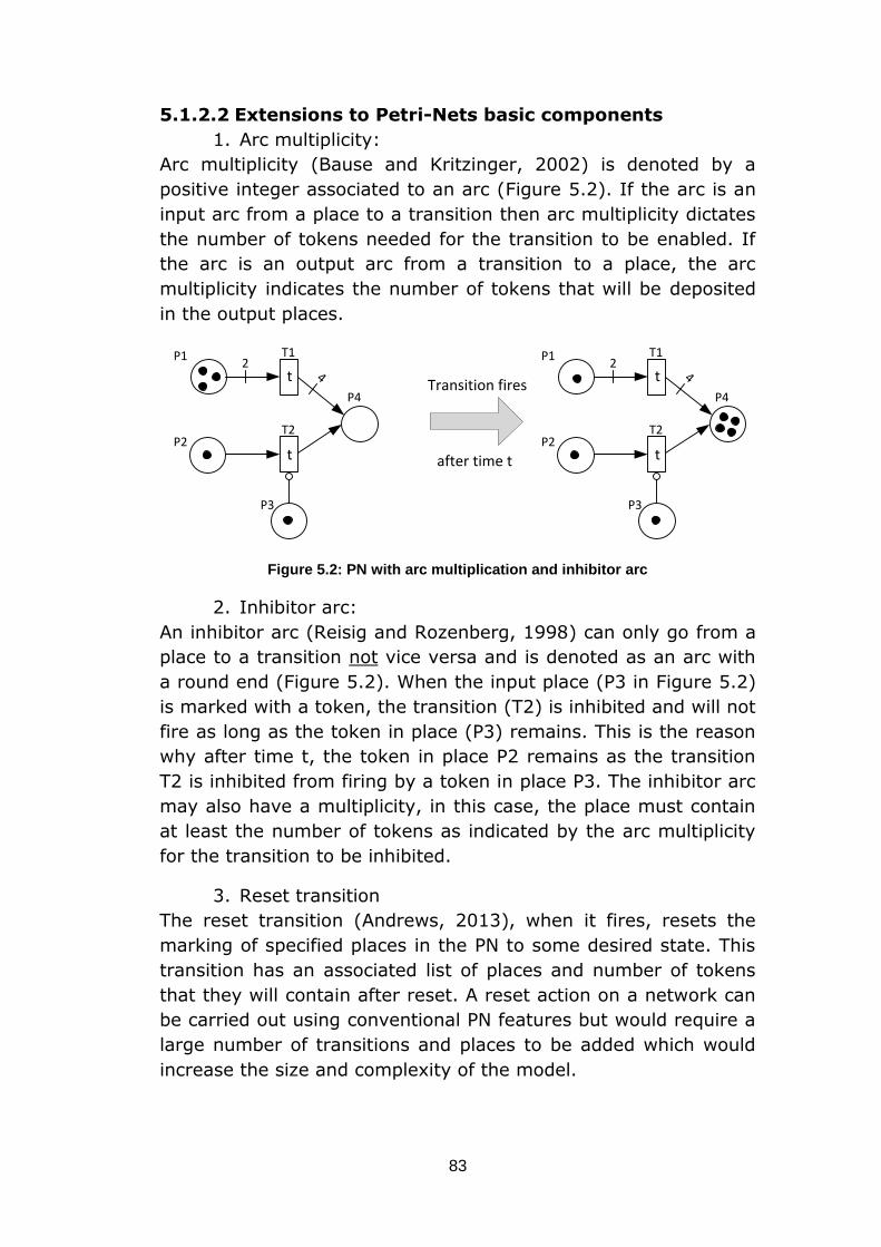
83
5.1.2.2 Extensions to Petri-Nets basic components
1. Arc multiplicity:
Arc multiplicity (Bause and Kritzinger, 2002) is denoted by a
positive integer associated to an arc (Figure 5.2). If the arc is an
input arc from a place to a transition then arc multiplicity dictates
the number of tokens needed for the transition to be enabled. If
the arc is an output arc from a transition to a place, the arc
multiplicity indicates the number of tokens that will be deposited
in the output places.
Figure 5.2: PN with arc multiplication and inhibitor arc
2. Inhibitor arc:
An inhibitor arc (Reisig and Rozenberg, 1998) can only go from a
place to a transition not vice versa and is denoted as an arc with
a round end (Figure 5.2). When the input place (P3 in Figure 5.2)
is marked with a token, the transition (T2) is inhibited and will not
fire as long as the token in place (P3) remains. This is the reason
why after time t, the token in place P2 remains as the transition
T2 is inhibited from firing by a token in place P3. The inhibitor arc
may also have a multiplicity, in this case, the place must contain
at least the number of tokens as indicated by the arc multiplicity
for the transition to be inhibited.
3. Reset transition
The reset transition (Andrews, 2013), when it fires, resets the
marking of specified places in the PN to some desired state. This
transition has an associated list of places and number of tokens
that they will contain after reset. A reset action on a network can
be carried out using conventional PN features but would require a
large number of transitions and places to be added which would
increase the size and complexity of the model.
Transition fires
after time tt
t2
4
t
t2
4
P1
P2
P3
P4
T1
T2
P1
P2
P3
P4
T1
T2
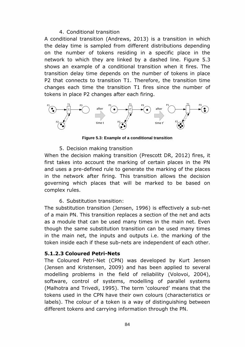
84
4. Conditional transition
A conditional transition (Andrews, 2013) is a transition in which
the delay time is sampled from different distributions depending
on the number of tokens residing in a specific place in the
network to which they are linked by a dashed line. Figure 5.3
shows an example of a conditional transition when it fires. The
transition delay time depends on the number of tokens in place
P2 that connects to transition T1. Therefore, the transition time
changes each time the transition T1 fires since the number of
tokens in place P2 changes after each firing.
Figure 5.3: Example of a conditional transition
5. Decision making transition
When the decision making transition (Prescott DR, 2012) fires, it
first takes into account the marking of certain places in the PN
and uses a pre-defined rule to generate the marking of the places
in the network after firing. This transition allows the decision
governing which places that will be marked to be based on
complex rules.
6. Substitution transition:
The substitution transition (Jensen, 1996) is effectively a sub-net
of a main PN. This transition replaces a section of the net and acts
as a module that can be used many times in the main net. Even
though the same substitution transition can be used many times
in the main net, the inputs and outputs i.e. the marking of the
token inside each if these sub-nets are independent of each other.
5.1.2.3 Coloured Petri-Nets
The Coloured Petri-Net (CPN) was developed by Kurt Jensen
(Jensen and Kristensen, 2009) and has been applied to several
modelling problems in the field of reliability (Volovoi, 2004),
software, control of systems, modelling of parallel systems
(Malhotra and Trivedi, 1995). The term ‘coloured’ means that the
tokens used in the CPN have their own colours (characteristics or
labels). The colour of a token is a way of distinguishing between
different tokens and carrying information through the PN.
t
P1 P3T1
P2 time t
after t'
P1 P3T1
P2 time t’
afterP1 P3T1
P2
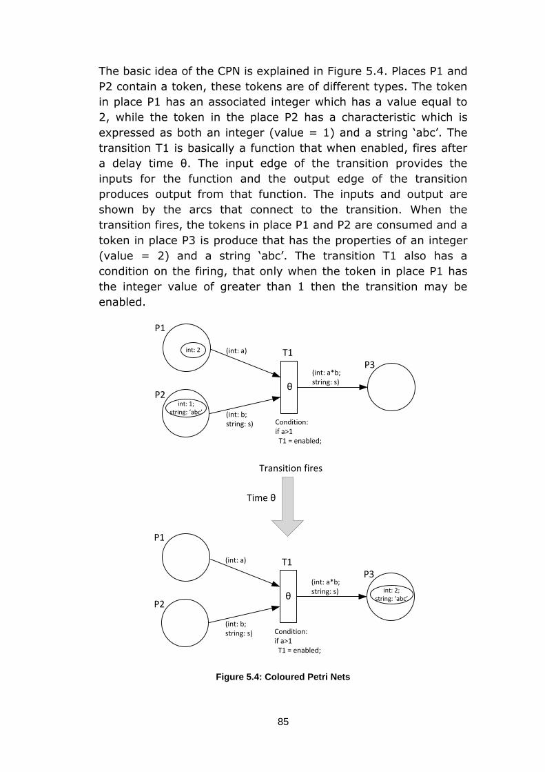
85
The basic idea of the CPN is explained in Figure 5.4. Places P1 and
P2 contain a token, these tokens are of different types. The token
in place P1 has an associated integer which has a value equal to
2, while the token in the place P2 has a characteristic which is
expressed as both an integer (value = 1) and a string ‘abc’. The
transition T1 is basically a function that when enabled, fires after
a delay time θ. The input edge of the transition provides the
inputs for the function and the output edge of the transition
produces output from that function. The inputs and output are
shown by the arcs that connect to the transition. When the
transition fires, the tokens in place P1 and P2 are consumed and a
token in place P3 is produce that has the properties of an integer
(value = 2) and a string ‘abc’. The transition T1 also has a
condition on the firing, that only when the token in place P1 has
the integer value of greater than 1 then the transition may be
enabled.
Figure 5.4: Coloured Petri Nets
Transition fires
Time θ
Condition:if a>1 T1 = enabled;
P3
P1
T1
P2
(int: a)
(int: b;string: s)
(int: a*b;string: s) int: 2;
string: ‘abc’θ
Condition:if a>1 T1 = enabled;
P3
P1
T1int: 2
int: 1;string: ‘abc’
P2
(int: a)
(int: b;string: s)
(int: a*b;string: s)
θ

86
In the CPN, the basic concept of the original PN is preserved. The
difference in the CPN is that, since the transition is now a
function, it is possible for the characteristics of the token to
change once it passes through a transition. Whereas, in the
traditional PN, the tokens are simply consumed at the input and
reproduced at the output of a transition. The flexibility and
advantage of the CPN comes from the ability to transform part of
the PN into a function. Thus, the flexibility of the PN can be
further enhanced by modifying part of the net (such as the arc) to
contain a function that effects the token in the desired way.
5.2 Model definitions
The PN used in this project can be regarded as an extension to
the traditional PN. The most important characteristic in the PN
used in this project is that each token is treated separately and
they each contain a set of properties that is unique to each bridge
component being modelled. Part of the net is modified to suit the
problem in bridge asset management. These improvisations are
discussed below.
5.2.1 Token
Each token used in the PN represents a particular bridge element.
A token carries a set of properties with it. Each token is unique
with an associated ID. The properties stored inside a token are as
follows:
a. Token ID
b. Component type/name
c. Component material
d. Coating condition
e. Environmental factor
f. Repair history (all repairs have happened and the
time at which they were carried out)
5.2.2 Place
A place denoted by a circle represents the state of the bridge
component.
5.2.3 Transition
a) Conditional transition
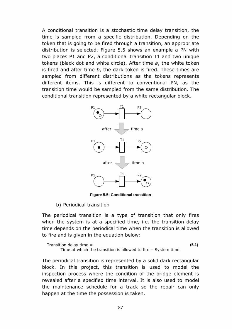
87
A conditional transition is a stochastic time delay transition, the
time is sampled from a specific distribution. Depending on the
token that is going to be fired through a transition, an appropriate
distribution is selected. Figure 5.5 shows an example a PN with
two places P1 and P2, a conditional transition T1 and two unique
tokens (black dot and white circle). After time a, the white token
is fired and after time b, the dark token is fired. These times are
sampled from different distributions as the tokens represents
different items. This is different to conventional PN, as the
transition time would be sampled from the same distribution. The
conditional transition represented by a white rectangular block.
Figure 5.5: Conditional transition
b) Periodical transition
The periodical transition is a type of transition that only fires
when the system is at a specified time, i.e. the transition delay
time depends on the periodical time when the transition is allowed
to fire and is given in the equation below:
Transition delay time =
Time at which the transition is allowed to fire – System time
(5.1)
The periodical transition is represented by a solid dark rectangular
block. In this project, this transition is used to model the
inspection process where the condition of the bridge element is
revealed after a specified time interval. It is also used to model
the maintenance schedule for a track so the repair can only
happen at the time the possession is taken.
P1 P2T1
P1 P2T1
time aafter
P1 P2T1
time bafter
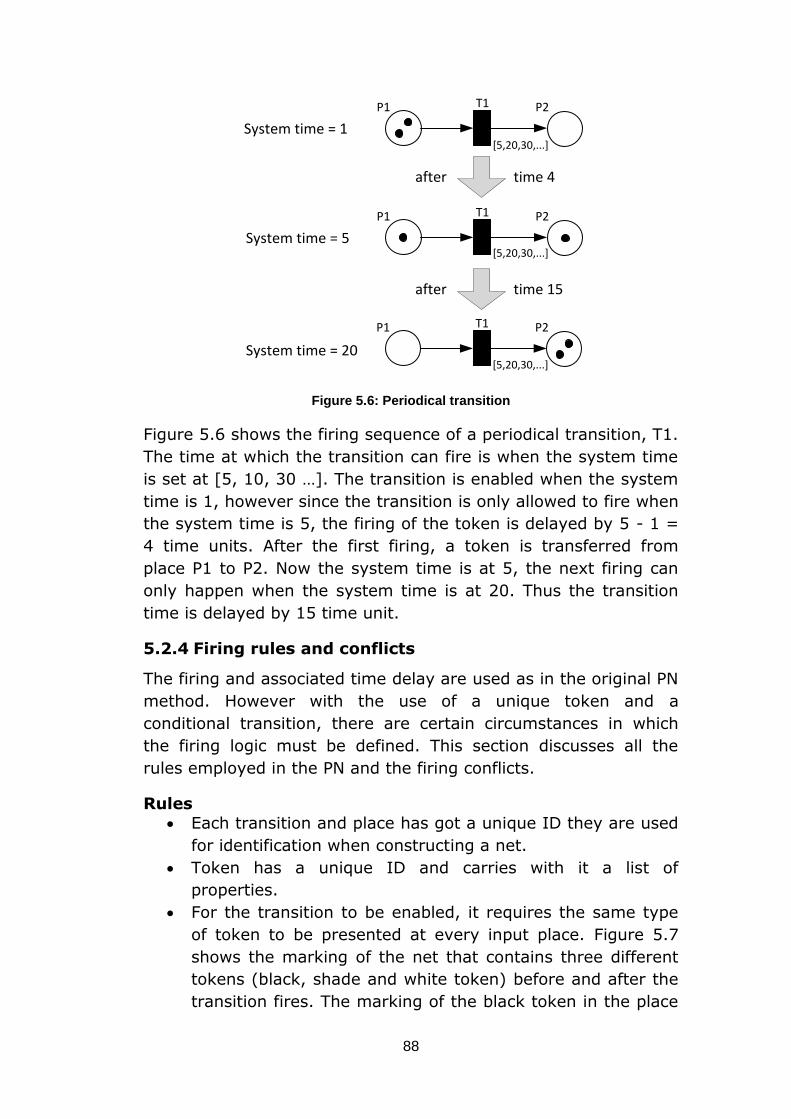
88
Figure 5.6: Periodical transition
Figure 5.6 shows the firing sequence of a periodical transition, T1.
The time at which the transition can fire is when the system time
is set at [5, 10, 30 …]. The transition is enabled when the system
time is 1, however since the transition is only allowed to fire when
the system time is 5, the firing of the token is delayed by 5 - 1 =
4 time units. After the first firing, a token is transferred from
place P1 to P2. Now the system time is at 5, the next firing can
only happen when the system time is at 20. Thus the transition
time is delayed by 15 time unit.
5.2.4 Firing rules and conflicts
The firing and associated time delay are used as in the original PN
method. However with the use of a unique token and a
conditional transition, there are certain circumstances in which
the firing logic must be defined. This section discusses all the
rules employed in the PN and the firing conflicts.
Rules
Each transition and place has got a unique ID they are used
for identification when constructing a net.
Token has a unique ID and carries with it a list of
properties.
For the transition to be enabled, it requires the same type
of token to be presented at every input place. Figure 5.7
shows the marking of the net that contains three different
tokens (black, shade and white token) before and after the
transition fires. The marking of the black token in the place
P1 P2T1
P1 P2T1
time 4after
time 15after
P1 P2T1
System time = 1
System time = 5
System time = 20
[5,20,30,...]
[5,20,30,...]
[5,20,30,...]
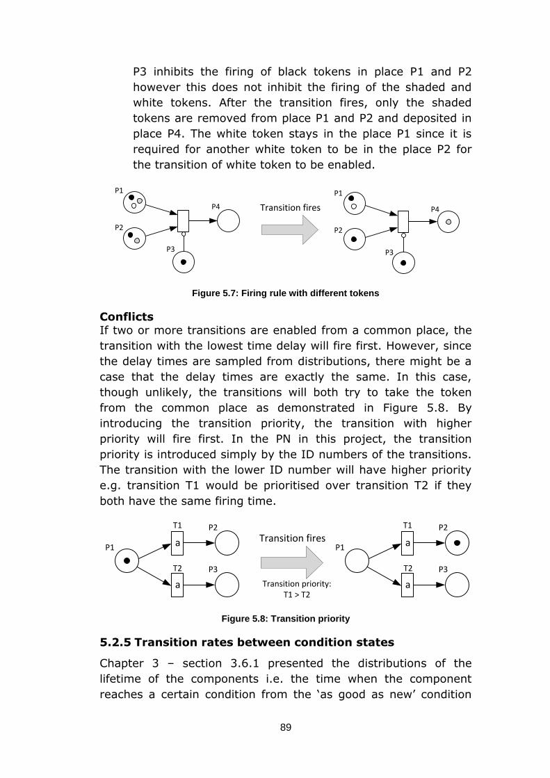
89
P3 inhibits the firing of black tokens in place P1 and P2
however this does not inhibit the firing of the shaded and
white tokens. After the transition fires, only the shaded
tokens are removed from place P1 and P2 and deposited in
place P4. The white token stays in the place P1 since it is
required for another white token to be in the place P2 for
the transition of white token to be enabled.
Figure 5.7: Firing rule with different tokens
Conflicts If two or more transitions are enabled from a common place, the
transition with the lowest time delay will fire first. However, since
the delay times are sampled from distributions, there might be a
case that the delay times are exactly the same. In this case,
though unlikely, the transitions will both try to take the token
from the common place as demonstrated in Figure 5.8. By
introducing the transition priority, the transition with higher
priority will fire first. In the PN in this project, the transition
priority is introduced simply by the ID numbers of the transitions.
The transition with the lower ID number will have higher priority
e.g. transition T1 would be prioritised over transition T2 if they
both have the same firing time.
Figure 5.8: Transition priority
5.2.5 Transition rates between condition states
Chapter 3 – section 3.6.1 presented the distributions of the
lifetime of the components i.e. the time when the component
reaches a certain condition from the ‘as good as new’ condition
P3
Transition fires
P1
P2
P4
P3
P1
P2
P4
P1
P2
P3
T1
T2
Transition firesa
a
P1
P2
P3
T1
T2
a
aTransition priority: T1 > T2
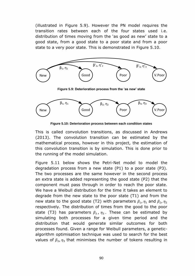
90
(illustrated in Figure 5.9). However the PN model requires the
transition rates between each of the four states used i.e.
distribution of times moving from the ‘as good as new’ state to a
good state, from a good state to a poor state and from a poor
state to a very poor state. This is demonstrated in Figure 5.10.
Figure 5.9: Deterioration process from the ‘as new’ state
Figure 5.10: Deterioration process between each condition states
This is called convolution transitions, as discussed in Andrews
(2013). The convolution transition can be estimated by the
mathematical process, however in this project, the estimation of
this convolution transition is by simulation. This is done prior to
the running of the model simulation.
Figure 5.11 below shows the Petri-Net model to model the
degradation process from a new state (P1) to a poor state (P3).
The two processes are the same however in the second process
an extra state is added representing the good state (P2) that the
component must pass through in order to reach the poor state.
We have a Weibull distribution for the time it takes an element to
degrade from the new state to the poor state (T1) and from the
new state to the good state (T2) with parameters , and ,
respectively. The distribution of times from the good to the poor
state (T3) has parameters , . These can be estimated by
simulating both processes for a given time period and the
distribution that would generate similar outcomes for both
processes found. Given a range for Weibull parameters, a genetic-
algorithm optimisation technique was used to search for the best
values of , that minimises the number of tokens resulting in
New Good Poor V.Poor
β'2, η’2 β'3, η’3β1, η1
New Good Poor V.Poor
β1, η1 β2, η2β3, η3
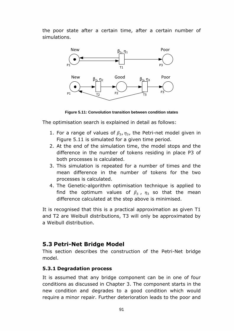
91
the poor state after a certain time, after a certain number of
simulations.
Figure 5.11: Convolution transition between condition states
The optimisation search is explained in detail as follows:
1. For a range of values of , , the Petri-net model given in
Figure 5.11 is simulated for a given time period.
2. At the end of the simulation time, the model stops and the
difference in the number of tokens residing in place P3 of
both processes is calculated.
3. This simulation is repeated for a number of times and the
mean difference in the number of tokens for the two
processes is calculated.
4. The Genetic-algorithm optimisation technique is applied to
find the optimum values of , so that the mean
difference calculated at the step above is minimised.
It is recognised that this is a practical approximation as given T1
and T2 are Weibull distributions, T3 will only be approximated by
a Weibull distribution.
5.3 Petri-Net Bridge Model
This section describes the construction of the Petri-Net bridge
model.
5.3.1 Degradation process
It is assumed that any bridge component can be in one of four
conditions as discussed in Chapter 3. The component starts in the
new condition and degrades to a good condition which would
require a minor repair. Further deterioration leads to the poor and
New Good Poor
New Poorβ1, η1
β2, η2 β3, η3
P1 P3
P3P1 P2
T1
T2 T3
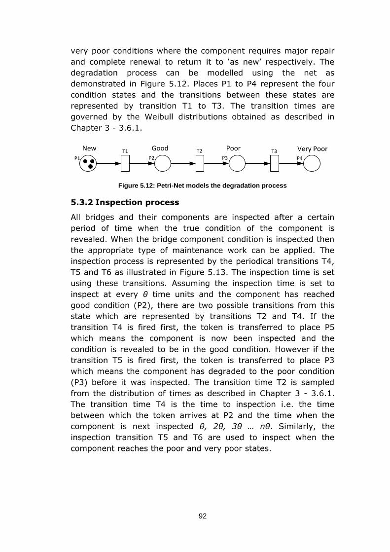
92
very poor conditions where the component requires major repair
and complete renewal to return it to ‘as new’ respectively. The
degradation process can be modelled using the net as
demonstrated in Figure 5.12. Places P1 to P4 represent the four
condition states and the transitions between these states are
represented by transition T1 to T3. The transition times are
governed by the Weibull distributions obtained as described in
Chapter 3 - 3.6.1.
Figure 5.12: Petri-Net models the degradation process
5.3.2 Inspection process
All bridges and their components are inspected after a certain
period of time when the true condition of the component is
revealed. When the bridge component condition is inspected then
the appropriate type of maintenance work can be applied. The
inspection process is represented by the periodical transitions T4,
T5 and T6 as illustrated in Figure 5.13. The inspection time is set
using these transitions. Assuming the inspection time is set to
inspect at every θ time units and the component has reached
good condition (P2), there are two possible transitions from this
state which are represented by transitions T2 and T4. If the
transition T4 is fired first, the token is transferred to place P5
which means the component is now been inspected and the
condition is revealed to be in the good condition. However if the
transition T5 is fired first, the token is transferred to place P3
which means the component has degraded to the poor condition
(P3) before it was inspected. The transition time T2 is sampled
from the distribution of times as described in Chapter 3 - 3.6.1.
The transition time T4 is the time to inspection i.e. the time
between which the token arrives at P2 and the time when the
component is next inspected θ, 2θ, 3θ … nθ. Similarly, the
inspection transition T5 and T6 are used to inspect when the
component reaches the poor and very poor states.
New Good Poor Very PoorP2P1 P3 P4
T1 T2 T3
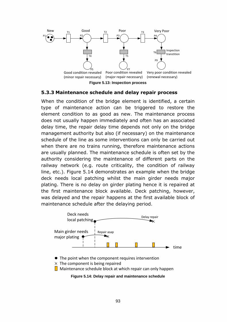
93
Figure 5.13: Inspection process
5.3.3 Maintenance schedule and delay repair process
When the condition of the bridge element is identified, a certain
type of maintenance action can be triggered to restore the
element condition to as good as new. The maintenance process
does not usually happen immediately and often has an associated
delay time, the repair delay time depends not only on the bridge
management authority but also (if necessary) on the maintenance
schedule of the line as some interventions can only be carried out
when there are no trains running, therefore maintenance actions
are usually planned. The maintenance schedule is often set by the
authority considering the maintenance of different parts on the
railway network (e.g. route criticality, the condition of railway
line, etc.). Figure 5.14 demonstrates an example when the bridge
deck needs local patching whilst the main girder needs major
plating. There is no delay on girder plating hence it is repaired at
the first maintenance block available. Deck patching, however,
was delayed and the repair happens at the first available block of
maintenance schedule after the delaying period.
time
Maintenance schedule block at which repair can only happen
Main girder needs major plating
Deck needs local patching
Repair asap
Delay repair
The point when the component requires interventionThe component is being repaired
Figure 5.14: Delay repair and maintenance schedule
New Good Poor Very Poor
Good condition revealed(minor repair necessary)
Inspection transtition
P2P1 P3 P4
P5 P7
P9
T1 T2 T3
T4 T5
T6
Poor condition revealed(major repair necessary)
Very poor condition revealed(renewal necessary)
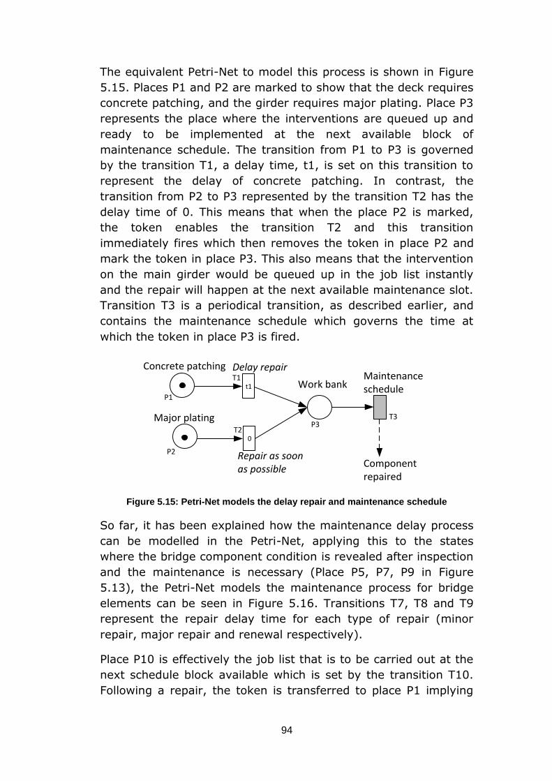
94
The equivalent Petri-Net to model this process is shown in Figure
5.15. Places P1 and P2 are marked to show that the deck requires
concrete patching, and the girder requires major plating. Place P3
represents the place where the interventions are queued up and
ready to be implemented at the next available block of
maintenance schedule. The transition from P1 to P3 is governed
by the transition T1, a delay time, t1, is set on this transition to
represent the delay of concrete patching. In contrast, the
transition from P2 to P3 represented by the transition T2 has the
delay time of 0. This means that when the place P2 is marked,
the token enables the transition T2 and this transition
immediately fires which then removes the token in place P2 and
mark the token in place P3. This also means that the intervention
on the main girder would be queued up in the job list instantly
and the repair will happen at the next available maintenance slot.
Transition T3 is a periodical transition, as described earlier, and
contains the maintenance schedule which governs the time at
which the token in place P3 is fired.
Major plating
Concrete patchingMaintenance scheduleWork bank
Delay repair
Repair as soon as possible
Component repaired
P1
P2
P3
T1
T2
T3
t1
0
Figure 5.15: Petri-Net models the delay repair and maintenance schedule
So far, it has been explained how the maintenance delay process
can be modelled in the Petri-Net, applying this to the states
where the bridge component condition is revealed after inspection
and the maintenance is necessary (Place P5, P7, P9 in Figure
5.13), the Petri-Net models the maintenance process for bridge
elements can be seen in Figure 5.16. Transitions T7, T8 and T9
represent the repair delay time for each type of repair (minor
repair, major repair and renewal respectively).
Place P10 is effectively the job list that is to be carried out at the
next schedule block available which is set by the transition T10.
Following a repair, the token is transferred to place P1 implying
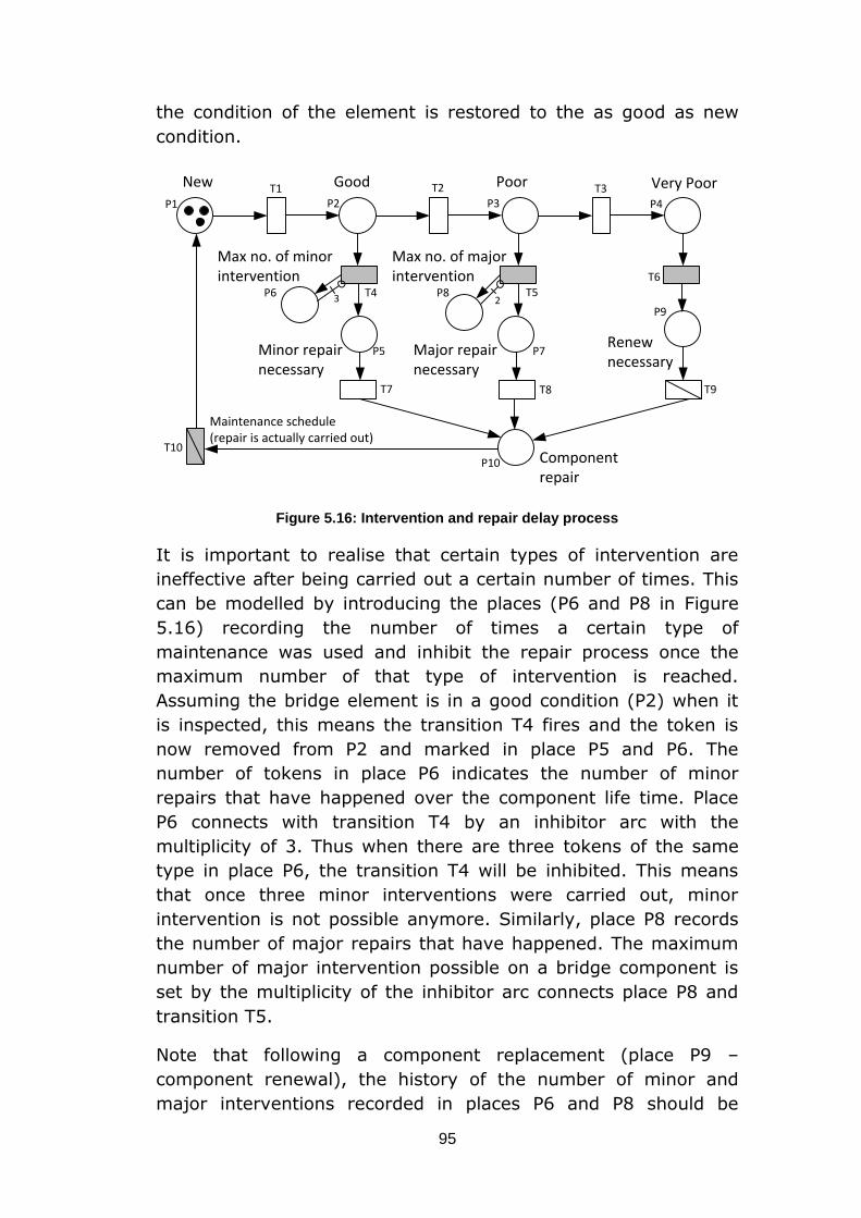
95
the condition of the element is restored to the as good as new
condition.
New Good Poor Very Poor
Max no. of minor intervention
Max no. of major intervention
Minor repair necessary
Major repair necessary
Renew necessary
Component repair
Maintenance schedule (repair is actually carried out)
P2P1 P3 P4
P6
P5
P8
P7
P9
T1 T2 T3
T4 T5
T6
T7 T8 T9
T10
P10
3 2
Figure 5.16: Intervention and repair delay process
It is important to realise that certain types of intervention are
ineffective after being carried out a certain number of times. This
can be modelled by introducing the places (P6 and P8 in Figure
5.16) recording the number of times a certain type of
maintenance was used and inhibit the repair process once the
maximum number of that type of intervention is reached.
Assuming the bridge element is in a good condition (P2) when it
is inspected, this means the transition T4 fires and the token is
now removed from P2 and marked in place P5 and P6. The
number of tokens in place P6 indicates the number of minor
repairs that have happened over the component life time. Place
P6 connects with transition T4 by an inhibitor arc with the
multiplicity of 3. Thus when there are three tokens of the same
type in place P6, the transition T4 will be inhibited. This means
that once three minor interventions were carried out, minor
intervention is not possible anymore. Similarly, place P8 records
the number of major repairs that have happened. The maximum
number of major intervention possible on a bridge component is
set by the multiplicity of the inhibitor arc connects place P8 and
transition T5.
Note that following a component replacement (place P9 –
component renewal), the history of the number of minor and
major interventions recorded in places P6 and P8 should be

96
cleared as this does not relate to the newly replaced component.
This is implemented in the model by using the reset transition T9.
When this transition fires, the tokens in places P6 and P8 are
cleared. It can be seen that transition T10 is also a reset
transition, when this transition fires, it resets the condition of the
coating, paint, protective layer etc. of the bridge element. This
will be explained in more detail in the next section.
5.3.4 Opportunistic maintenance
New Good Poor Very Poor
Minor repair scheduled
Major repair scheduled
Renewal scheduled
P2P1 P3 P4
P5 P7 P9
T1 T2 T3
T4 T5 T6
0
T11
0
T12
0
T13
P19
Enable opportunistic maintenance
Figure 5.17: Petri-net module representing opportunistic maintenance
Figure 5.17 illustrates the PN representation to model the
opportunistic maintenance. There are black, green, yellow and red
tokens that model four bridge main girders. The red token is in
the place P9 where it is scheduled for a renewal, this means that
one girder is in the poor condition and after the inspection where
its condition is revealed, the girder will be replaced. The other
girders represented by the black, green and yellow tokens are
currently in the good and poor states. Opportunistic maintenance
considers carrying out minor and major repairs on the black,
green and yellow tokens. This is modelled by introducing
transitions T12 and T13. The red and yellow tokens enable
transition T12 and after the transition fires, the yellow token is
transferred to place P7 where it is scheduled for a major repair.
The red token is cleared from place P9 when the transition fires
but is then deposited back in place P9 immediately after the firing
as indicating by the double ended arc connecting place P9 to
transition T12. Similarly, the red, black and green tokens now
enable the transition T13 which transfers the green and the black
token into place P5 which indicates a minor repair will be carried
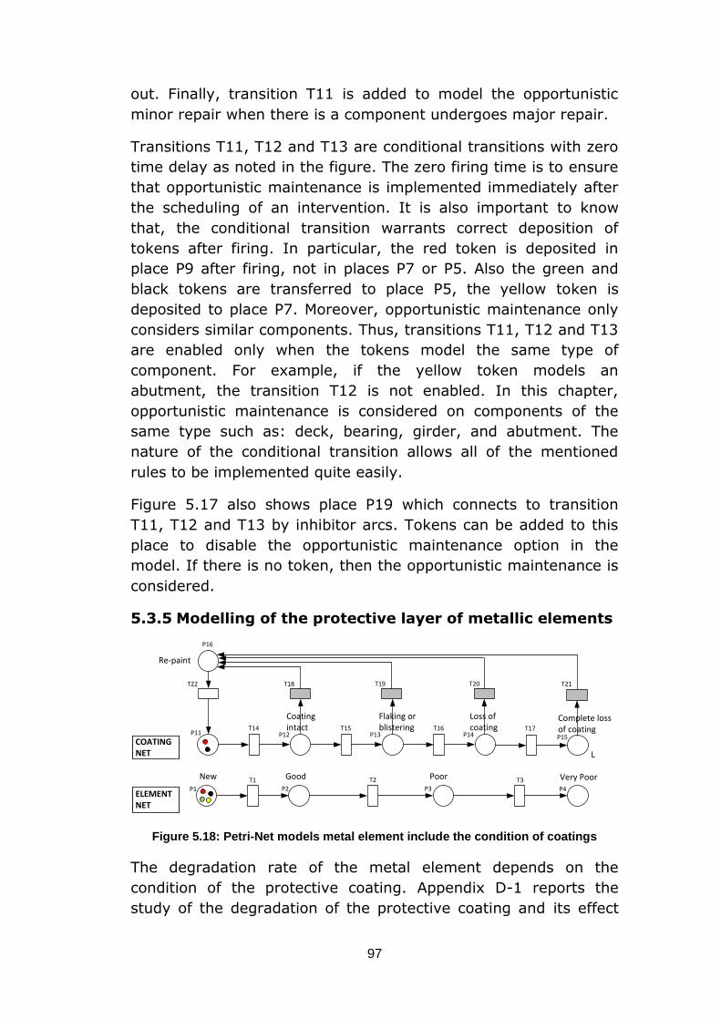
97
out. Finally, transition T11 is added to model the opportunistic
minor repair when there is a component undergoes major repair.
Transitions T11, T12 and T13 are conditional transitions with zero
time delay as noted in the figure. The zero firing time is to ensure
that opportunistic maintenance is implemented immediately after
the scheduling of an intervention. It is also important to know
that, the conditional transition warrants correct deposition of
tokens after firing. In particular, the red token is deposited in
place P9 after firing, not in places P7 or P5. Also the green and
black tokens are transferred to place P5, the yellow token is
deposited to place P7. Moreover, opportunistic maintenance only
considers similar components. Thus, transitions T11, T12 and T13
are enabled only when the tokens model the same type of
component. For example, if the yellow token models an
abutment, the transition T12 is not enabled. In this chapter,
opportunistic maintenance is considered on components of the
same type such as: deck, bearing, girder, and abutment. The
nature of the conditional transition allows all of the mentioned
rules to be implemented quite easily.
Figure 5.17 also shows place P19 which connects to transition
T11, T12 and T13 by inhibitor arcs. Tokens can be added to this
place to disable the opportunistic maintenance option in the
model. If there is no token, then the opportunistic maintenance is
considered.
5.3.5 Modelling of the protective layer of metallic elements
New Good Poor Very PoorP2P1 P3 P4
T1 T2 T3
ELEMENTNET
COATING NET L
Coating intact
Flaking or blistering
Loss of coating
Complete loss of coating
Re-paint
P11 P12 P13 P14 P15
P16
T14 T15 T16 T17
T21T20T19T18T22
Figure 5.18: Petri-Net models metal element include the condition of coatings
The degradation rate of the metal element depends on the
condition of the protective coating. Appendix D-1 reports the
study of the degradation of the protective coating and its effect

98
on the deterioration rate of its protected metal. It is possible to
capture and model this effect in the PN bridge model. Figure 5.18
shows two separate Petri-nets, the top net models the condition
of the coating and the bottom net models the condition of the
metal element itself. The bottom net should extend to be the
same as the net presented in Figure 5.16, however, only part of
the net is illustrated here. There are five coating conditions which
are represented by places P11 to P15. The transitions between
these conditions are represented by transitions T14 to T17.
Transitions T18 to T21 are periodical transitions which are used to
model the inspection process where the condition of the coating is
revealed following an inspection. It is assumed that if the coating
condition is revealed to be in the state where there is some loss
(P14) or a complete loss of coating (P15) then the component will
be re-painted (P16) and the condition of the coating will be
restored to the new condition.
Even though the two nets are separated however the modelling of
the deterioration processes of the element and its coating are
dependent. This is modelled by connecting the token in both nets
through their characteristics. In the net PN1, the position of the
token updates that token property. This property i.e. the current
condition of the coating is therefore also captured in the token in
the net PN2. Based on the property of the token, an appropriate
degradation rate is chosen to model the deterioration of the metal
element in the net PN2.
As mentioned previously, the transition T10 in the net PN2 is a
reset transition (transition T10 can be seen in Figure 5.16). When
this transition fires, it resets the net PN1 by removing the token
in any place in the net and marks the token in place P11. This
reset action in the model implies that when the repair happens on
the metal element, the coating of that element is also restored to
new condition.
5.3.6 Bridge model
5.3.6.1 Intervention options
The intervention strategy can be set by placing tokens into places
P17 and P18 in the Petri-Net as demonstrated in Figure 5.19.
These places inhibit the transitions T4 and T5, thus disable a
certain type of repairs for a bridge component. In this way the
intervention strategy can be applied differently on each bridge
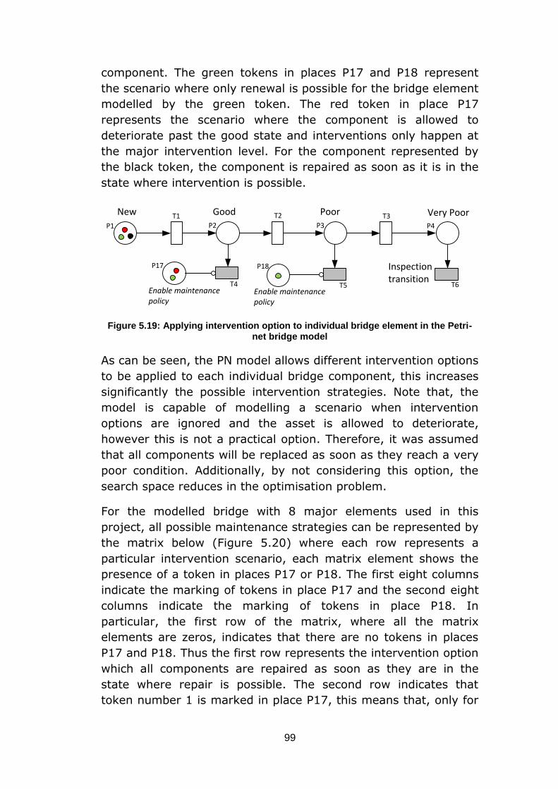
99
component. The green tokens in places P17 and P18 represent
the scenario where only renewal is possible for the bridge element
modelled by the green token. The red token in place P17
represents the scenario where the component is allowed to
deteriorate past the good state and interventions only happen at
the major intervention level. For the component represented by
the black token, the component is repaired as soon as it is in the
state where intervention is possible.
New Good Poor Very PoorP2P1 P3 P4
P17 P18
T1 T2 T3
T4 T5 T6Enable maintenance policy
Enable maintenance policy
Inspectiontransition
Figure 5.19: Applying intervention option to individual bridge element in the Petri-net bridge model
As can be seen, the PN model allows different intervention options
to be applied to each individual bridge component, this increases
significantly the possible intervention strategies. Note that, the
model is capable of modelling a scenario when intervention
options are ignored and the asset is allowed to deteriorate,
however this is not a practical option. Therefore, it was assumed
that all components will be replaced as soon as they reach a very
poor condition. Additionally, by not considering this option, the
search space reduces in the optimisation problem.
For the modelled bridge with 8 major elements used in this
project, all possible maintenance strategies can be represented by
the matrix below (Figure 5.20) where each row represents a
particular intervention scenario, each matrix element shows the
presence of a token in places P17 or P18. The first eight columns
indicate the marking of tokens in place P17 and the second eight
columns indicate the marking of tokens in place P18. In
particular, the first row of the matrix, where all the matrix
elements are zeros, indicates that there are no tokens in places
P17 and P18. Thus the first row represents the intervention option
which all components are repaired as soon as they are in the
state where repair is possible. The second row indicates that
token number 1 is marked in place P17, this means that, only for
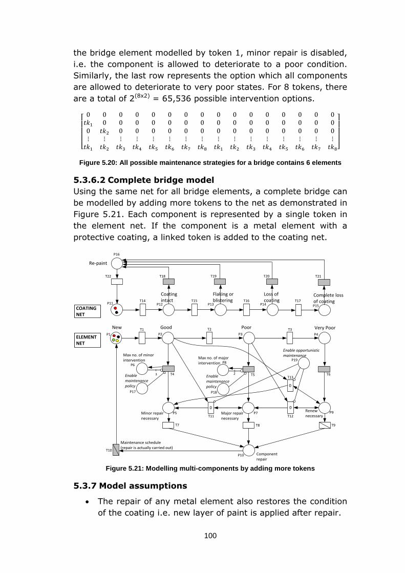
100
the bridge element modelled by token 1, minor repair is disabled,
i.e. the component is allowed to deteriorate to a poor condition.
Similarly, the last row represents the option which all components
are allowed to deteriorate to very poor states. For 8 tokens, there
are a total of 2(8x2) = 65,536 possible intervention options.
[
]
Figure 5.20: All possible maintenance strategies for a bridge contains 6 elements
5.3.6.2 Complete bridge model
Using the same net for all bridge elements, a complete bridge can
be modelled by adding more tokens to the net as demonstrated in
Figure 5.21. Each component is represented by a single token in
the element net. If the component is a metal element with a
protective coating, a linked token is added to the coating net.
New Good Poor Very Poor
Max no. of minor intervention
Max no. of major intervention
Minor repair necessary
Major repair necessary
Renew necessary
Component repair
Maintenance schedule (repair is actually carried out)
P2P1 P3 P4
P6
P5
P8
P7 P9
T1 T2 T3
T4 T5 T6
T7 T8 T9
T10
P10
3 2
ELEMENTNET
COATING NET
Coating intact
Flaking or blistering
Loss of coating
Complete loss of coating
Re-paint
P11 P12 P13 P14 P15
P16
T14 T15 T16 T17
T21T20T19T18T22
P17
Enable maintenance policy
P18
Enable maintenance policy
0
T11
0
T12
0
T13
P19
Enable opportunistic maintenance
Figure 5.21: Modelling multi-components by adding more tokens
5.3.7 Model assumptions
The repair of any metal element also restores the condition
of the coating i.e. new layer of paint is applied after repair.
101
Inspections are assumed to be perfect, that is, the real
element deterioration state can be detected without error.
Maintenance is also modelled as perfect that is a repair will
restore the system to the ‘as good as new’ condition.
5.4 Model analysis
5.4.1 Model construction and simulation
So far, a PN model has been formulated to model the dynamic
process of the change in states of a bridge asset. The net changes
state when an event occurs and for many stochastic process
modelled in the net, these changes occur at random time.
Simulation is required to simulate all of the changes in the
system. Therefore, the developed PN bridge model provides a
framework for simulation where many processes and rules are
incorporated.
There are several commercially available programs that can
simulate the PN model, however, due to the modifications to the
original PN modelling technique, a computer program was written
to accommodate the generation and solution of the PN bridge
model. The model is used to simulate the bridge and its elements’
conditions and the effects of maintenance over a 60 year lifetime
period.
5.4.2 Monte Carlo sampling
Sampling from distributions is required for all stochastic
transitions. For all the transitions that are governed by a Weibull
distribution, Weibull(η,β), the transition times are derived by
generating a random probability and the sampled transition time
is calculated using the equation below:
( ( ))
(5.2)
where
t is the sample time
X is a random number between 0 and 1
The random sampling process is repeated for a number of times
(number of simulations) and statistics are collected. These
statistics indicate the performance and characteristics of the
system. The PN bridge model allows many types of characteristics
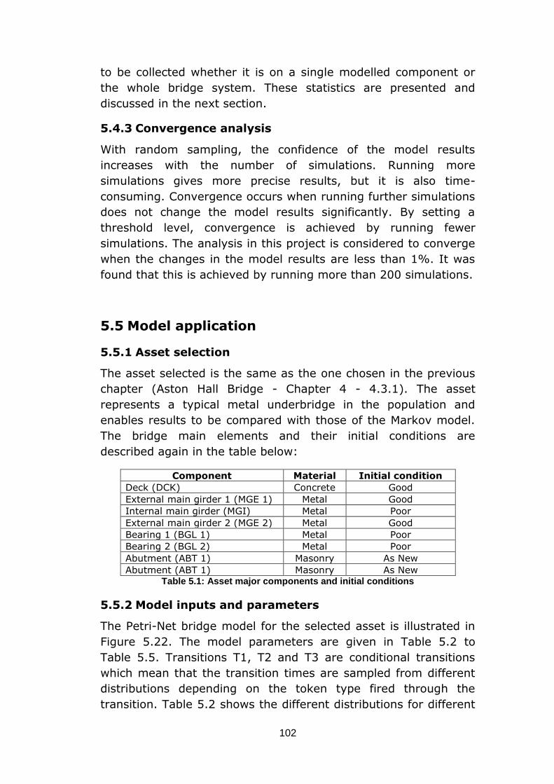
102
to be collected whether it is on a single modelled component or
the whole bridge system. These statistics are presented and
discussed in the next section.
5.4.3 Convergence analysis
With random sampling, the confidence of the model results
increases with the number of simulations. Running more
simulations gives more precise results, but it is also time-
consuming. Convergence occurs when running further simulations
does not change the model results significantly. By setting a
threshold level, convergence is achieved by running fewer
simulations. The analysis in this project is considered to converge
when the changes in the model results are less than 1%. It was
found that this is achieved by running more than 200 simulations.
5.5 Model application
5.5.1 Asset selection
The asset selected is the same as the one chosen in the previous
chapter (Aston Hall Bridge - Chapter 4 - 4.3.1). The asset
represents a typical metal underbridge in the population and
enables results to be compared with those of the Markov model.
The bridge main elements and their initial conditions are
described again in the table below:
Component Material Initial condition
Deck (DCK) Concrete Good
External main girder 1 (MGE 1) Metal Good
Internal main girder (MGI) Metal Poor
External main girder 2 (MGE 2) Metal Good
Bearing 1 (BGL 1) Metal Poor
Bearing 2 (BGL 2) Metal Poor
Abutment (ABT 1) Masonry As New
Abutment (ABT 1) Masonry As New Table 5.1: Asset major components and initial conditions
5.5.2 Model inputs and parameters
The Petri-Net bridge model for the selected asset is illustrated in
Figure 5.22. The model parameters are given in Table 5.2 to
Table 5.5. Transitions T1, T2 and T3 are conditional transitions
which mean that the transition times are sampled from different
distributions depending on the token type fired through the
transition. Table 5.2 shows the different distributions for different
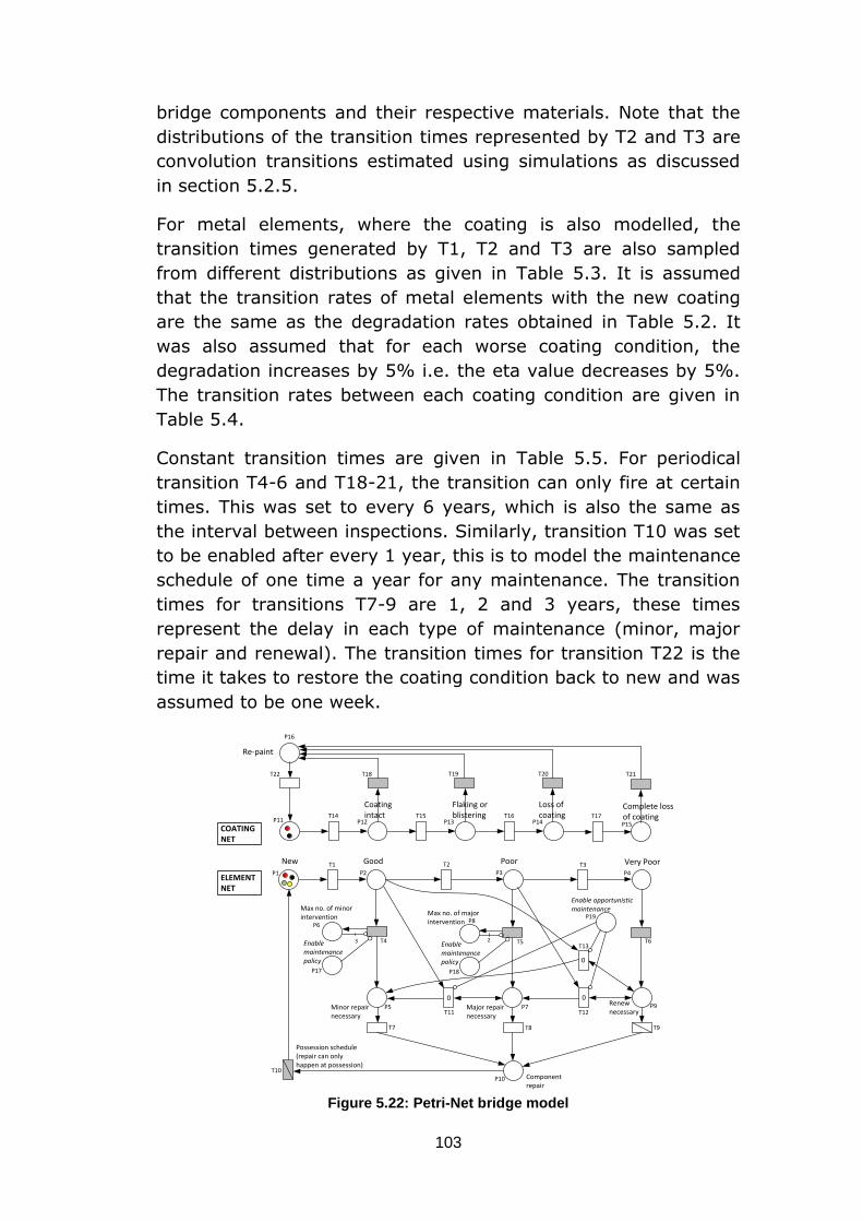
103
bridge components and their respective materials. Note that the
distributions of the transition times represented by T2 and T3 are
convolution transitions estimated using simulations as discussed
in section 5.2.5.
For metal elements, where the coating is also modelled, the
transition times generated by T1, T2 and T3 are also sampled
from different distributions as given in Table 5.3. It is assumed
that the transition rates of metal elements with the new coating
are the same as the degradation rates obtained in Table 5.2. It
was also assumed that for each worse coating condition, the
degradation increases by 5% i.e. the eta value decreases by 5%.
The transition rates between each coating condition are given in
Table 5.4.
Constant transition times are given in Table 5.5. For periodical
transition T4-6 and T18-21, the transition can only fire at certain
times. This was set to every 6 years, which is also the same as
the interval between inspections. Similarly, transition T10 was set
to be enabled after every 1 year, this is to model the maintenance
schedule of one time a year for any maintenance. The transition
times for transitions T7-9 are 1, 2 and 3 years, these times
represent the delay in each type of maintenance (minor, major
repair and renewal). The transition times for transition T22 is the
time it takes to restore the coating condition back to new and was
assumed to be one week.
New Good Poor Very Poor
Max no. of minor intervention
Max no. of major intervention
Minor repair necessary
Major repair necessary
Renew necessary
Component repair
Possession schedule(repair can only happen at possession)
P2P1 P3 P4
P6
P5
P8
P7 P9
T1 T2 T3
T4 T5 T6
T7 T8 T9
T10
P10
3 2
ELEMENTNET
COATING NET
Coating intact
Flaking or blistering
Loss of coating
Complete loss of coating
Re-paint
P11 P12 P13 P14 P15
P16
T14 T15 T16 T17
T21T20T19T18T22
P17
Enable maintenance policy
P18
Enable maintenance policy
0
T11
0
T12
0
T13
P19
Enable opportunistic maintenance
Figure 5.22: Petri-Net bridge model
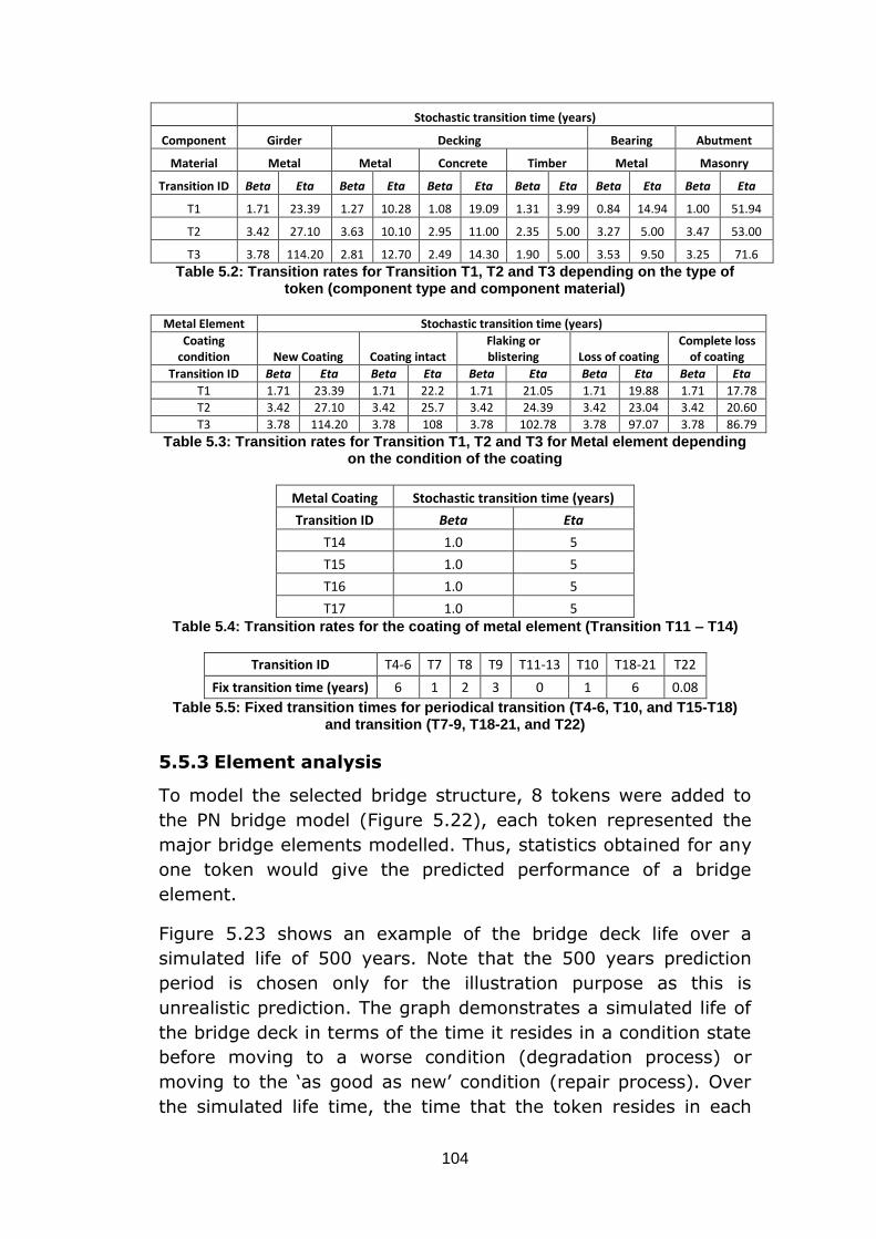
104
Stochastic transition time (years)
Component Girder Decking Bearing Abutment
Material Metal Metal Concrete Timber Metal Masonry
Transition ID Beta Eta Beta Eta Beta Eta Beta Eta Beta Eta Beta Eta
T1 1.71 23.39 1.27 10.28 1.08 19.09 1.31 3.99 0.84 14.94 1.00 51.94
T2 3.42 27.10 3.63 10.10 2.95 11.00 2.35 5.00 3.27 5.00 3.47 53.00
T3 3.78 114.20 2.81 12.70 2.49 14.30 1.90 5.00 3.53 9.50 3.25 71.6
Table 5.2: Transition rates for Transition T1, T2 and T3 depending on the type of token (component type and component material)
Metal Element Stochastic transition time (years)
Coating condition New Coating Coating intact
Flaking or blistering Loss of coating
Complete loss of coating
Transition ID Beta Eta Beta Eta Beta Eta Beta Eta Beta Eta
T1 1.71 23.39 1.71 22.2 1.71 21.05 1.71 19.88 1.71 17.78
T2 3.42 27.10 3.42 25.7 3.42 24.39 3.42 23.04 3.42 20.60
T3 3.78 114.20 3.78 108 3.78 102.78 3.78 97.07 3.78 86.79
Table 5.3: Transition rates for Transition T1, T2 and T3 for Metal element depending on the condition of the coating
Metal Coating Stochastic transition time (years)
Transition ID Beta Eta
T14 1.0 5
T15 1.0 5
T16 1.0 5
T17 1.0 5 Table 5.4: Transition rates for the coating of metal element (Transition T11 – T14)
Transition ID T4-6 T7 T8 T9 T11-13 T10 T18-21 T22
Fix transition time (years) 6 1 2 3 0 1 6 0.08
Table 5.5: Fixed transition times for periodical transition (T4-6, T10, and T15-T18) and transition (T7-9, T18-21, and T22)
5.5.3 Element analysis
To model the selected bridge structure, 8 tokens were added to
the PN bridge model (Figure 5.22), each token represented the
major bridge elements modelled. Thus, statistics obtained for any
one token would give the predicted performance of a bridge
element.
Figure 5.23 shows an example of the bridge deck life over a
simulated life of 500 years. Note that the 500 years prediction
period is chosen only for the illustration purpose as this is
unrealistic prediction. The graph demonstrates a simulated life of
the bridge deck in terms of the time it resides in a condition state
before moving to a worse condition (degradation process) or
moving to the ‘as good as new’ condition (repair process). Over
the simulated life time, the time that the token resides in each
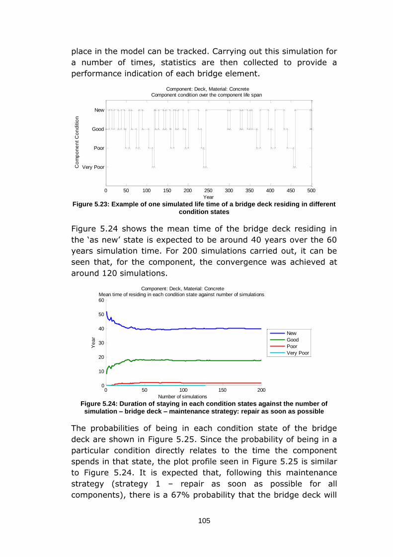
105
place in the model can be tracked. Carrying out this simulation for
a number of times, statistics are then collected to provide a
performance indication of each bridge element.
Figure 5.23: Example of one simulated life time of a bridge deck residing in different
condition states
Figure 5.24 shows the mean time of the bridge deck residing in
the ‘as new’ state is expected to be around 40 years over the 60
years simulation time. For 200 simulations carried out, it can be
seen that, for the component, the convergence was achieved at
around 120 simulations.
Figure 5.24: Duration of staying in each condition states against the number of
simulation – bridge deck – maintenance strategy: repair as soon as possible
The probabilities of being in each condition state of the bridge
deck are shown in Figure 5.25. Since the probability of being in a
particular condition directly relates to the time the component
spends in that state, the plot profile seen in Figure 5.25 is similar
to Figure 5.24. It is expected that, following this maintenance
strategy (strategy 1 – repair as soon as possible for all
components), there is a 67% probability that the bridge deck will
0 50 100 150 200 250 300 350 400 450 500
Very Poor
Poor
Good
New
Year
Co
mp
on
en
t C
on
ditio
n
Component: Deck, Material: ConcreteComponent condition over the component life span
0 50 100 150 2000
10
20
30
40
50
60
Number of simulations
Ye
ar
Component: Deck, Material: ConcreteMean time of residing in each condition state against number of simulations
New
Good
Poor
Very Poor
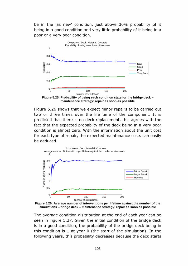
106
be in the ‘as new’ condition, just above 30% probability of it
being in a good condition and very little probability of it being in a
poor or a very poor condition.
Figure 5.25: Probability of being each condition state for the bridge deck –
maintenance strategy: repair as soon as possible
Figure 5.26 shows that we expect minor repairs to be carried out
two or three times over the life time of the component. It is
predicted that there is no deck replacement, this agrees with the
fact that the expected probabilty of the deck being in a very poor
condition is almost zero. With the information about the unit cost
for each type of repair, the expected maintenance costs can easily
be deduced.
Figure 5.26: Average number of interventions per lifetime against the number of the
simulations – bridge deck – maintenance strategy: repair as soon as possible
The average condition disitribution at the end of each year can be
seen in Figure 5.27. Given the initial condition of the bridge deck
is in a good condition, the probability of the bridge deck being in
this condition is 1 at year 0 (the start of the simulation). In the
following years, this probability decreases because the deck starts
0 50 100 150 2000
0.2
0.4
0.6
0.8
1
Number of simulations
Pro
ba
bili
tyComponent: Deck, Material: Concrete
Probability of being in each condition state
New
Good
Poor
Very Poor
0 50 100 150 2000
0.5
1
1.5
2
2.5
3
Number of simulations
Nu
mb
er
of
inte
rve
ntio
ns
Component: Deck, Material: ConcreteAverage number of interventions per lifetime against the number of simulatons
Minor Repair
Major Repair
Renewal
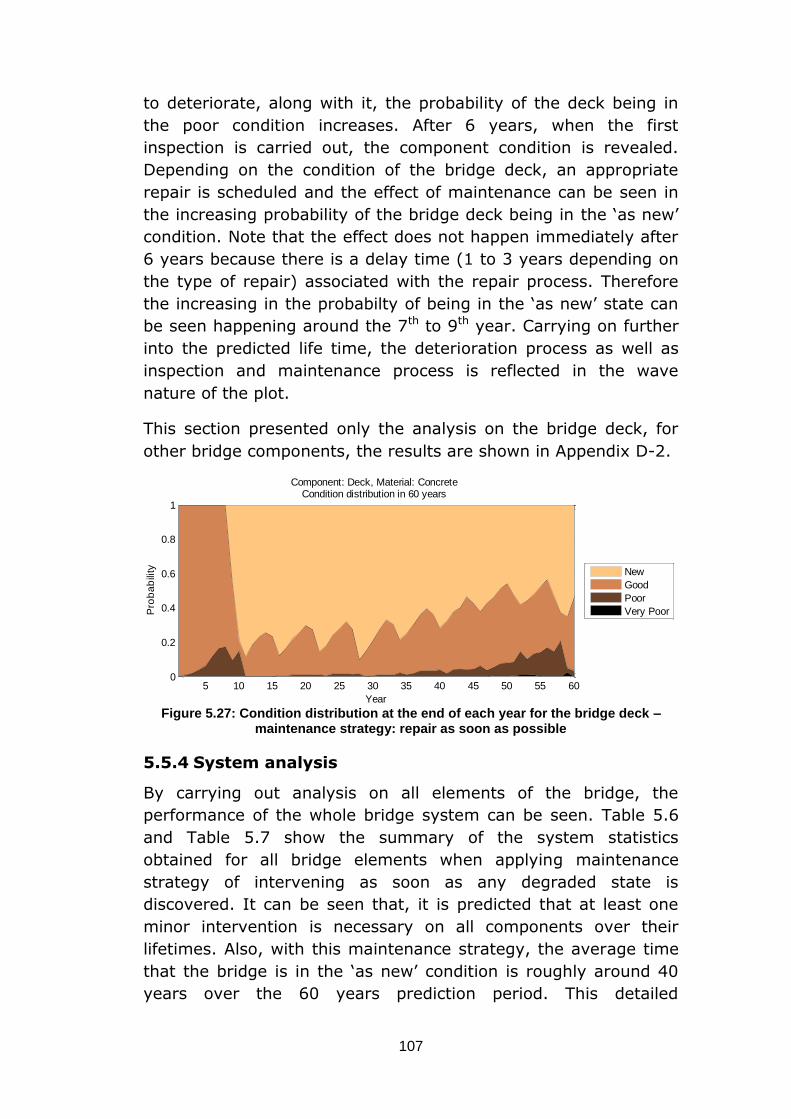
107
to deteriorate, along with it, the probability of the deck being in
the poor condition increases. After 6 years, when the first
inspection is carried out, the component condition is revealed.
Depending on the condition of the bridge deck, an appropriate
repair is scheduled and the effect of maintenance can be seen in
the increasing probability of the bridge deck being in the ‘as new’
condition. Note that the effect does not happen immediately after
6 years because there is a delay time (1 to 3 years depending on
the type of repair) associated with the repair process. Therefore
the increasing in the probabilty of being in the ‘as new’ state can
be seen happening around the 7th to 9th year. Carrying on further
into the predicted life time, the deterioration process as well as
inspection and maintenance process is reflected in the wave
nature of the plot.
This section presented only the analysis on the bridge deck, for
other bridge components, the results are shown in Appendix D-2.
Figure 5.27: Condition distribution at the end of each year for the bridge deck –
maintenance strategy: repair as soon as possible
5.5.4 System analysis
By carrying out analysis on all elements of the bridge, the
performance of the whole bridge system can be seen. Table 5.6
and Table 5.7 show the summary of the system statistics
obtained for all bridge elements when applying maintenance
strategy of intervening as soon as any degraded state is
discovered. It can be seen that, it is predicted that at least one
minor intervention is necessary on all components over their
lifetimes. Also, with this maintenance strategy, the average time
that the bridge is in the ‘as new’ condition is roughly around 40
years over the 60 years prediction period. This detailed
5 10 15 20 25 30 35 40 45 50 55 600
0.2
0.4
0.6
0.8
1
Year
Pro
ba
bili
ty
Component: Deck, Material: ConcreteCondition distribution in 60 years
New
Good
Poor
Very Poor
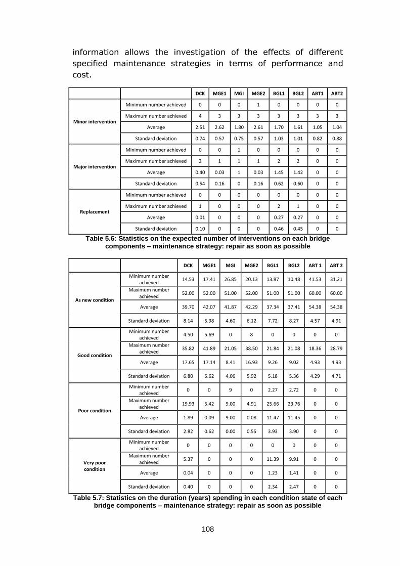
108
information allows the investigation of the effects of different
specified maintenance strategies in terms of performance and
cost.
DCK MGE1 MGI MGE2 BGL1 BGL2 ABT1 ABT2
Minor intervention
Minimum number achieved 0 0 0 1 0 0 0 0
Maximum number achieved 4 3 3 3 3 3 3 3
Average 2.51 2.62 1.80 2.61 1.70 1.61 1.05 1.04
Standard deviation 0.74 0.57 0.75 0.57 1.03 1.01 0.82 0.88
Major intervention
Minimum number achieved 0 0 1 0 0 0 0 0
Maximum number achieved 2 1 1 1 2 2 0 0
Average 0.40 0.03 1 0.03 1.45 1.42 0 0
Standard deviation 0.54 0.16 0 0.16 0.62 0.60 0 0
Replacement
Minimum number achieved 0 0 0 0 0 0 0 0
Maximum number achieved 1 0 0 0 2 1 0 0
Average 0.01 0 0 0 0.27 0.27 0 0
Standard deviation 0.10 0 0 0 0.46 0.45 0 0
Table 5.6: Statistics on the expected number of interventions on each bridge components – maintenance strategy: repair as soon as possible
DCK MGE1 MGI MGE2 BGL1 BGL2 ABT 1 ABT 2
As new condition
Minimum number achieved
14.53 17.41 26.85 20.13 13.87 10.48 41.53 31.21
Maximum number achieved
52.00 52.00 51.00 52.00 51.00 51.00 60.00 60.00
Average 39.70 42.07 41.87 42.29 37.34 37.41 54.38 54.38
Standard deviation 8.14 5.98 4.60 6.12 7.72 8.27 4.57 4.91
Good condition
Minimum number achieved
4.50 5.69 0 8 0 0 0 0
Maximum number achieved
35.82 41.89 21.05 38.50 21.84 21.08 18.36 28.79
Average 17.65 17.14 8.41 16.93 9.26 9.02 4.93 4.93
Standard deviation 6.80 5.62 4.06 5.92 5.18 5.36 4.29 4.71
Poor condition
Minimum number achieved
0 0 9 0 2.27 2.72 0 0
Maximum number achieved
19.93 5.42 9.00 4.91 25.66 23.76 0 0
Average 1.89 0.09 9.00 0.08 11.47 11.45 0 0
Standard deviation 2.82 0.62 0.00 0.55 3.93 3.90 0 0
Very poor condition
Minimum number achieved
0 0 0 0 0 0 0 0
Maximum number achieved
5.37 0 0 0 11.39 9.91 0 0
Average 0.04 0 0 0 1.23 1.41 0 0
Standard deviation 0.40 0 0 0 2.34 2.47 0 0
Table 5.7: Statistics on the duration (years) spending in each condition state of each bridge components – maintenance strategy: repair as soon as possible
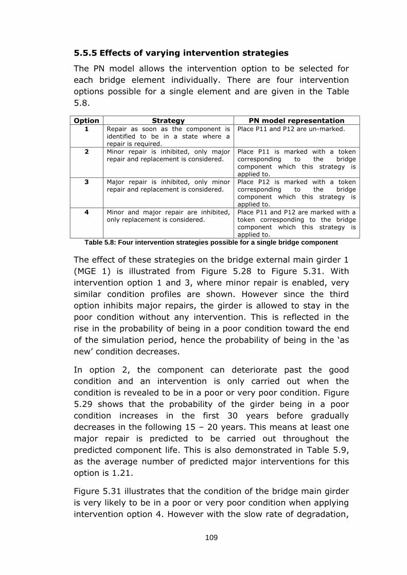
109
5.5.5 Effects of varying intervention strategies
The PN model allows the intervention option to be selected for
each bridge element individually. There are four intervention
options possible for a single element and are given in the Table
5.8.
Option Strategy PN model representation 1 Repair as soon as the component is
identified to be in a state where a repair is required.
Place P11 and P12 are un-marked.
2 Minor repair is inhibited, only major repair and replacement is considered.
Place P11 is marked with a token corresponding to the bridge
component which this strategy is
applied to.
3 Major repair is inhibited, only minor repair and replacement is considered.
Place P12 is marked with a token corresponding to the bridge component which this strategy is applied to.
4 Minor and major repair are inhibited, only replacement is considered.
Place P11 and P12 are marked with a token corresponding to the bridge component which this strategy is applied to.
Table 5.8: Four intervention strategies possible for a single bridge component
The effect of these strategies on the bridge external main girder 1
(MGE 1) is illustrated from Figure 5.28 to Figure 5.31. With
intervention option 1 and 3, where minor repair is enabled, very
similar condition profiles are shown. However since the third
option inhibits major repairs, the girder is allowed to stay in the
poor condition without any intervention. This is reflected in the
rise in the probability of being in a poor condition toward the end
of the simulation period, hence the probability of being in the ‘as
new’ condition decreases.
In option 2, the component can deteriorate past the good
condition and an intervention is only carried out when the
condition is revealed to be in a poor or very poor condition. Figure
5.29 shows that the probability of the girder being in a poor
condition increases in the first 30 years before gradually
decreases in the following 15 – 20 years. This means at least one
major repair is predicted to be carried out throughout the
predicted component life. This is also demonstrated in Table 5.9,
as the average number of predicted major interventions for this
option is 1.21.
Figure 5.31 illustrates that the condition of the bridge main girder
is very likely to be in a poor or very poor condition when applying
intervention option 4. However with the slow rate of degradation,
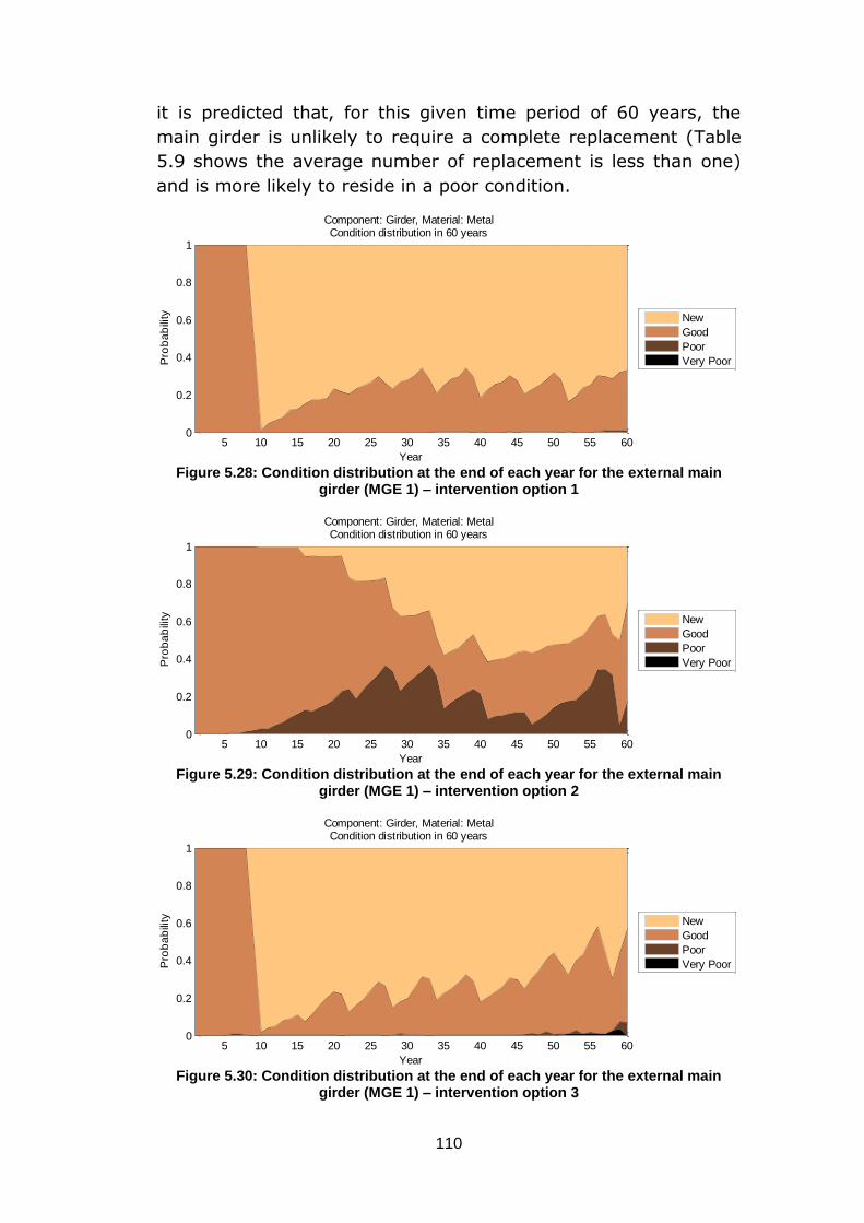
110
it is predicted that, for this given time period of 60 years, the
main girder is unlikely to require a complete replacement (Table
5.9 shows the average number of replacement is less than one)
and is more likely to reside in a poor condition.
Figure 5.28: Condition distribution at the end of each year for the external main
girder (MGE 1) – intervention option 1
Figure 5.29: Condition distribution at the end of each year for the external main
girder (MGE 1) – intervention option 2
Figure 5.30: Condition distribution at the end of each year for the external main
girder (MGE 1) – intervention option 3
5 10 15 20 25 30 35 40 45 50 55 600
0.2
0.4
0.6
0.8
1
Year
Pro
ba
bili
ty
Component: Girder, Material: MetalCondition distribution in 60 years
New
Good
Poor
Very Poor
5 10 15 20 25 30 35 40 45 50 55 600
0.2
0.4
0.6
0.8
1
Year
Pro
ba
bili
ty
Component: Girder, Material: MetalCondition distribution in 60 years
New
Good
Poor
Very Poor
5 10 15 20 25 30 35 40 45 50 55 600
0.2
0.4
0.6
0.8
1
Year
Pro
ba
bili
ty
Component: Girder, Material: MetalCondition distribution in 60 years
New
Good
Poor
Very Poor
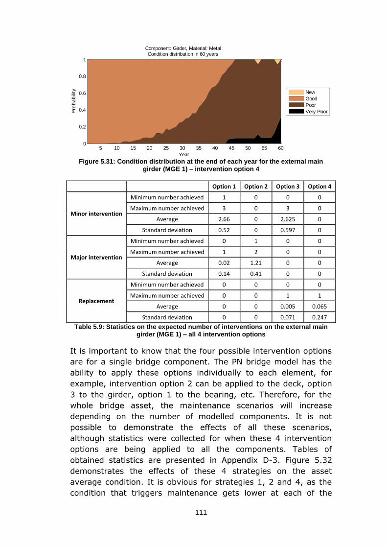
111
Figure 5.31: Condition distribution at the end of each year for the external main
girder (MGE 1) – intervention option 4
Option 1 Option 2 Option 3 Option 4
Minor intervention
Minimum number achieved 1 0 0 0
Maximum number achieved 3 0 3 0
Average 2.66 0 2.625 0
Standard deviation 0.52 0 0.597 0
Major intervention
Minimum number achieved 0 1 0 0
Maximum number achieved 1 2 0 0
Average 0.02 1.21 0 0
Standard deviation 0.14 0.41 0 0
Replacement
Minimum number achieved 0 0 0 0
Maximum number achieved 0 0 1 1
Average 0 0 0.005 0.065
Standard deviation 0 0 0.071 0.247
Table 5.9: Statistics on the expected number of interventions on the external main girder (MGE 1) – all 4 intervention options
It is important to know that the four possible intervention options
are for a single bridge component. The PN bridge model has the
ability to apply these options individually to each element, for
example, intervention option 2 can be applied to the deck, option
3 to the girder, option 1 to the bearing, etc. Therefore, for the
whole bridge asset, the maintenance scenarios will increase
depending on the number of modelled components. It is not
possible to demonstrate the effects of all these scenarios,
although statistics were collected for when these 4 intervention
options are being applied to all the components. Tables of
obtained statistics are presented in Appendix D-3. Figure 5.32
demonstrates the effects of these 4 strategies on the asset
average condition. It is obvious for strategies 1, 2 and 4, as the
condition that triggers maintenance gets lower at each of the
5 10 15 20 25 30 35 40 45 50 55 600
0.2
0.4
0.6
0.8
1
Year
Pro
ba
bili
ty
Component: Girder, Material: MetalCondition distribution in 60 years
New
Good
Poor
Very Poor
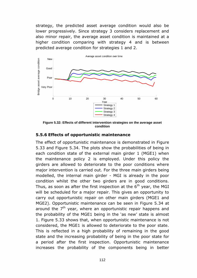
112
strategy, the predicted asset average condition would also be
lower progressively. Since strategy 3 considers replacement and
also minor repair, the average asset condition is maintained at a
higher condition comparing with strategy 4 and is between
predicted average condition for strategies 1 and 2.
Figure 5.32: Effects of different intervention strategies on the average asset
condition
5.5.6 Effects of opportunistic maintenance
The effect of opportunistic maintenance is demonstrated in Figure
5.33 and Figure 5.34. The plots show the probabilities of being in
each condition state of the external main girder 1 (MGE1) when
the maintenance policy 2 is employed. Under this policy the
girders are allowed to deteriorate to the poor conditions where
major intervention is carried out. For the three main girders being
modelled, the internal main girder - MGI is already in the poor
condition whilst the other two girders are in good conditions.
Thus, as soon as after the first inspection at the 6th year, the MGI
will be scheduled for a major repair. This gives an opportunity to
carry out opportunistic repair on other main girders (MGE1 and
MGE2). Opportunistic maintenance can be seen in Figure 5.34 at
around the 7th year, where an opportunistic repair happens and
the probability of the MGE1 being in the ‘as new’ state is almost
1. Figure 5.33 shows that, when opportunistic maintenance is not
considered, the MGE1 is allowed to deteriorate to the poor state.
This is reflected in a high probability of remaining in the good
state and the increasing probability of being in the poor state for
a period after the first inspection. Opportunistic maintenance
increases the probability of the components being in better
0 10 20 30 40 50 60
Very Poor
Poor
Good
New
Year
Bri
dg
e a
sse
t a
ve
rag
e c
on
ditio
n
Average asset condition over time
Strategy 1
Strategy 2
Strategy 3
Strategy 4
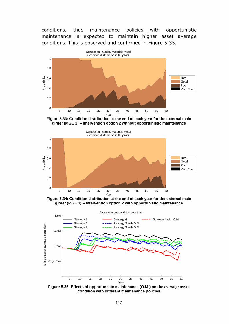
113
conditions, thus maintenance policies with opportunistic
maintenance is expected to maintain higher asset average
conditions. This is observed and confirmed in Figure 5.35.
Figure 5.33: Condition distribution at the end of each year for the external main
girder (MGE 1) – intervention option 2 without opportunistic maintenance
Figure 5.34: Condition distribution at the end of each year for the external main
girder (MGE 1) – intervention option 2 with opportunistic maintenance
Figure 5.35: Effects of opportunistic maintenance (O.M.) on the average asset
condition with different maintenance policies
5 10 15 20 25 30 35 40 45 50 55 600
0.2
0.4
0.6
0.8
1
Year
Pro
ba
bili
ty
Component: Girder, Material: MetalCondition distribution in 60 years
New
Good
Poor
Very Poor
5 10 15 20 25 30 35 40 45 50 55 600
0.2
0.4
0.6
0.8
1
Year
Pro
ba
bili
ty
Component: Girder, Material: MetalCondition distribution in 60 years
New
Good
Poor
Very Poor
5 10 15 20 25 30 35 40 45 50 55 60
Very Poor
Poor
Good
New
Year
Bri
dg
e a
sse
t a
ve
rag
e c
on
ditio
n
Average asset condition over time
Strategy 1
Strategy 2
Strategy 3
Strategy 4
Strategy 2 with O.M.
Strategy 3 with O.M.
Strategy 4 with O.M.
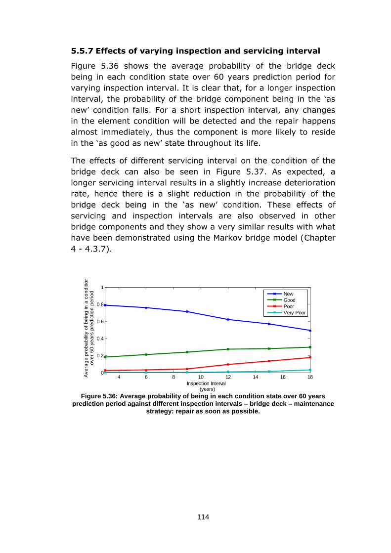
114
5.5.7 Effects of varying inspection and servicing interval
Figure 5.36 shows the average probability of the bridge deck
being in each condition state over 60 years prediction period for
varying inspection interval. It is clear that, for a longer inspection
interval, the probability of the bridge component being in the ‘as
new’ condition falls. For a short inspection interval, any changes
in the element condition will be detected and the repair happens
almost immediately, thus the component is more likely to reside
in the ‘as good as new’ state throughout its life.
The effects of different servicing interval on the condition of the
bridge deck can also be seen in Figure 5.37. As expected, a
longer servicing interval results in a slightly increase deterioration
rate, hence there is a slight reduction in the probability of the
bridge deck being in the ‘as new’ condition. These effects of
servicing and inspection intervals are also observed in other
bridge components and they show a very similar results with what
have been demonstrated using the Markov bridge model (Chapter
4 - 4.3.7).
Figure 5.36: Average probability of being in each condition state over 60 years
prediction period against different inspection intervals – bridge deck – maintenance strategy: repair as soon as possible.
4 6 8 10 12 14 16 180
0.2
0.4
0.6
0.8
1
Inspection Interval(years)
Ave
rag
e p
rob
ab
ility
of
be
ing
in
a c
on
ditio
no
ve
r 6
0 y
ea
rs p
red
ictio
n p
eri
od
New
Good
Poor
Very Poor
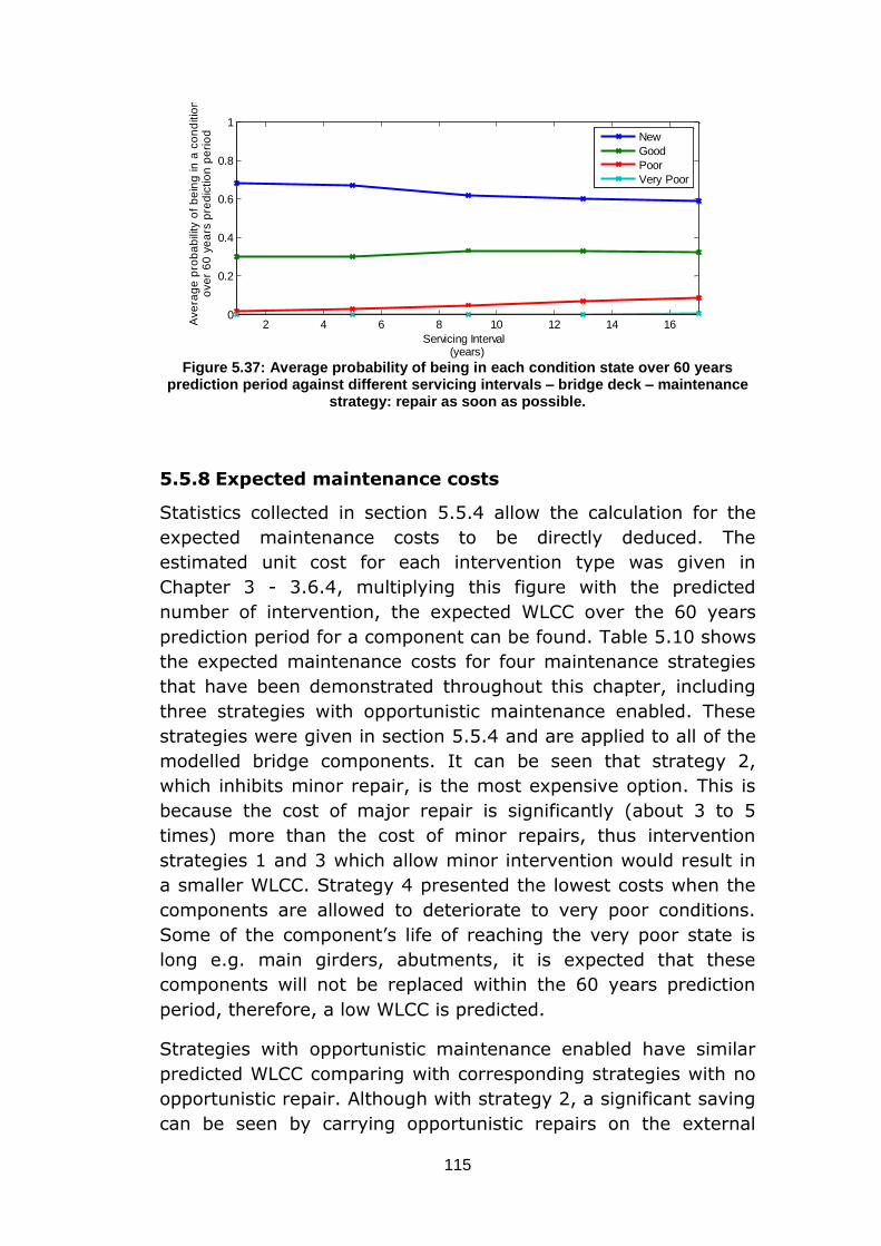
115
Figure 5.37: Average probability of being in each condition state over 60 years
prediction period against different servicing intervals – bridge deck – maintenance strategy: repair as soon as possible.
5.5.8 Expected maintenance costs
Statistics collected in section 5.5.4 allow the calculation for the
expected maintenance costs to be directly deduced. The
estimated unit cost for each intervention type was given in
Chapter 3 - 3.6.4, multiplying this figure with the predicted
number of intervention, the expected WLCC over the 60 years
prediction period for a component can be found. Table 5.10 shows
the expected maintenance costs for four maintenance strategies
that have been demonstrated throughout this chapter, including
three strategies with opportunistic maintenance enabled. These
strategies were given in section 5.5.4 and are applied to all of the
modelled bridge components. It can be seen that strategy 2,
which inhibits minor repair, is the most expensive option. This is
because the cost of major repair is significantly (about 3 to 5
times) more than the cost of minor repairs, thus intervention
strategies 1 and 3 which allow minor intervention would result in
a smaller WLCC. Strategy 4 presented the lowest costs when the
components are allowed to deteriorate to very poor conditions.
Some of the component’s life of reaching the very poor state is
long e.g. main girders, abutments, it is expected that these
components will not be replaced within the 60 years prediction
period, therefore, a low WLCC is predicted.
Strategies with opportunistic maintenance enabled have similar
predicted WLCC comparing with corresponding strategies with no
opportunistic repair. Although with strategy 2, a significant saving
can be seen by carrying opportunistic repairs on the external
2 4 6 8 10 12 14 160
0.2
0.4
0.6
0.8
1
Servicing Interval(years)
Ave
rag
e p
rob
ab
ility
of
be
ing
in
a c
on
ditio
no
ve
r 6
0 y
ea
rs p
red
ictio
n p
eri
od
New
Good
Poor
Very Poor

116
main girders and bearings. The opportunistic costs are reflected in
the cost of minor repairs for these components, offsetting these
costs against the saving in the major repair costs, the predicted
WLCC is actually cheaper by 9.3% with opportunistic
maintenance.
Strategy Intervention type DCK MGE1 MGI1 MGE2 BGL1 BGL2 ABT1 ABT2 Total
1
Minor repair 7455 16911 11024 17106 6615 7336 5423 5562
Major repair 3174 835 23861 1432 32272 32951 0 0
Renewal 0 0 0 0 12000 8600 0 0
Total 10629 17746 34885 18537 50887 48887 5423 5562 202106
2
Minor repair 0 0 0 0 0 0 0 0
Major repair 14689 28037 41876 28872 43935 45747 4150 5321
Renewal 2727 0 0 0 26400 30000 0 0
Total 17417 28037 41876 28872 70335 75747 4150 5321 281303
3
Minor repair 6631 16878 98 17171 5873 5938 5898 6373
Major repair 0 0 0 0 0 0 0 0
Renewal 6399 0 3536 0 58600 60400 0 0
Total 13030 16878 3633 17171 64473 66338 5898 6373 203344
4
Minor repair 0 0 0 0 0 0 0 0
Major repair 0 0 0 0 0 0 0 0
Renewal 27589 416 2912 1248 81200 80400 0 0
Total 27589 416 2912 1248 81200 80400 0 0 203315
2 with opportunistic maintenance
Minor repair 0 9789 3967 9561 1397 1812 587 671
Major repair 14364 11692 33047 13601 44954 45181 4150 4257
Renewal 3776 0 0 0 21200 21600 0 0
Total 18140 21480 37015 23162 67551 68593 4737 4927 255156
3 with opportunistic maintenance
Minor repair 6944 17333 293 17138 6572 6353 5702 6066
Major repair 0 0 119 0 5888 4416 0 0
Renewal 7763 0 4575 208 51000 53000 0 0
Total 14706 17333 4987 17346 63460 63769 5702 6066 202920
4 with opportunistic maintenance
Minor repair 0 0 0 0 589 415 0 0
Major repair 0 954 358 835 8832 6794 0 0
Renewal 27799 208 2288 624 72000 75600 0 400
Total 27799 1162 2646 1459 81422 82809 0 400 207247
Table 5.10: Expected WLCC for all bridge components for four maintenance strategies
Figure 5.38 shows the WLCC for each component under the four
maintenance strategies, the plots also show the contribution of
the expected costs for each intervention types. Similar
information is illustrated in Figure 5.39 for strategies 2-4 with
opportunistic maintenance. The plots clearly reflect the intention
of the intervention strategies, for example, Figure 5.38(c) shows
zero expected costs for major repair, this is because strategy 3
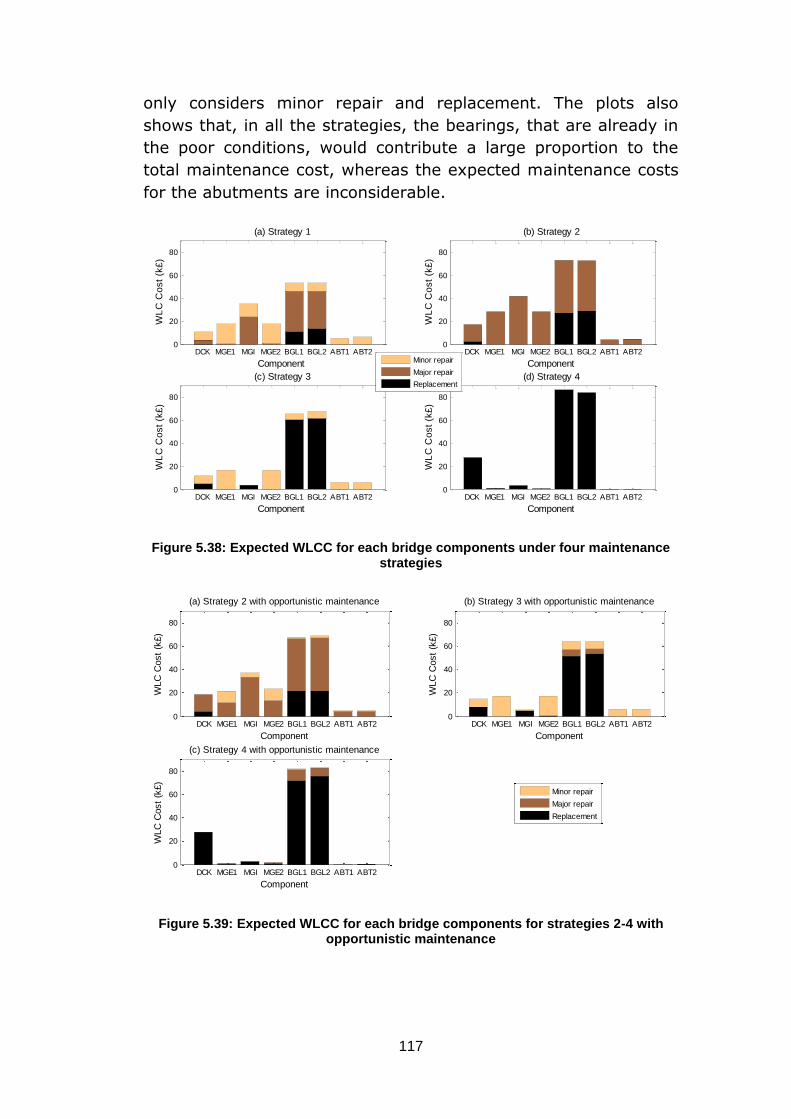
117
only considers minor repair and replacement. The plots also
shows that, in all the strategies, the bearings, that are already in
the poor conditions, would contribute a large proportion to the
total maintenance cost, whereas the expected maintenance costs
for the abutments are inconsiderable.
Figure 5.38: Expected WLCC for each bridge components under four maintenance strategies
Figure 5.39: Expected WLCC for each bridge components for strategies 2-4 with opportunistic maintenance
DCK MGE1 MGI MGE2 BGL1 BGL2 ABT1 ABT20
20
40
60
80
Component
WL
C C
ost
(k£
)
(a) Strategy 1
DCK MGE1 MGI MGE2 BGL1 BGL2 ABT1 ABT20
20
40
60
80
(b) Strategy 2
Component
WL
C C
ost
(k£
)
DCK MGE1 MGI MGE2 BGL1 BGL2 ABT1 ABT20
20
40
60
80
(c) Strategy 3
Component
WL
C C
ost
(k£
)
DCK MGE1 MGI MGE2 BGL1 BGL2 ABT1 ABT20
20
40
60
80
(d) Strategy 4
Component
WL
C C
ost
(k£
)
Minor repair
Major repair
Replacement
DCK MGE1 MGI MGE2 BGL1 BGL2 ABT1 ABT20
20
40
60
80
Component
WLC
Cost
(k£)
(a) Strategy 2 with opportunistic maintenance
DCK MGE1 MGI MGE2 BGL1 BGL2 ABT1 ABT20
20
40
60
80
(b) Strategy 3 with opportunistic maintenance
Component
WLC
Cost
(k£)
DCK MGE1 MGI MGE2 BGL1 BGL2 ABT1 ABT20
20
40
60
80
(c) Strategy 4 with opportunistic maintenance
Component
WLC
Cost
(k£)
Minor repair
Major repair
Replacement
118
5.6 Summary
This chapter described the development of a bridge model using
the Petri-Net modelling technique. The technique is increasingly
being used in modelling dynamic systems, and has never been
applied to model bridge assets. This chapter gives an overview of
the PN method before developing a PN bridge model. It also
discusses, in detail, the modifications to the original PN modelling
technique to suit the problem in modelling bridge asset
management. The model is then applied to the selected asset and
simulation results are presented and discussed.
The model inputs are the distributions of times that an element
degrades to a certain condition state. A Monte Carlo simulation
was used to simulate the model and statistics are then collected
to show the performance of bridge elements. The PN bridge
model developed is considered novel and it overcomes several
limitations in other bridge models based on Markov modelling. In
particular, the PN bridge model presented several advantages,
they are:
Non-constant deterioration rate,
Detail modelling of the component, e.g. model the coating
of metal component as well as the component itself,
Repair happens according to a specific maintenance
schedule set for a route (depends on the route criticality,
the number of planned maintenance block for a year is
usually limited),
Certain types of repairs are ineffective after a certain
number of times carried out,
Modularity properties of the PN model allow other type of
assets to be incorporated for across asset modelling.
119
Chapter 6 - Markov and Petri Net Model Comparison
6.1 Introduction
In the previous two chapters, two different bridge models have
been developed based on the Markov and the Petri-Net
techniques. The Petri-Net bridge model presented several
advantages that have addressed the limitations in the Markov
bridge model. The PN model not only offers a different approach
to the modelling of bridge assets and but also has the capability
to incorporate more detail. In this chapter, the results obtained by
the two modelling approaches are compared and discussed by
applying the same maintenance policy on the same selected
asset.
6.2 Predicting component future average condition
It is expected for the same asset, the average future asset
condition profile should be similar using the two models. Given
that the model inputs are the same and the same maintenance
policy is applied. In this section, the results obtained from the
models are investigated to establish if they indicate good
matches.
Figure 6.1 shows the predicted condition profile for the bridge
deck using the Markov model under a maintenance policy of
replacing only when the bridge component reaches the very poor
condition. The plot is obtained by progressing from the initial
condition in very small time steps over the 60 years prediction
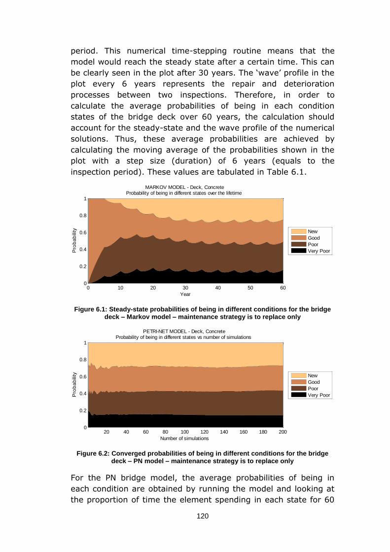
120
period. This numerical time-stepping routine means that the
model would reach the steady state after a certain time. This can
be clearly seen in the plot after 30 years. The ‘wave’ profile in the
plot every 6 years represents the repair and deterioration
processes between two inspections. Therefore, in order to
calculate the average probabilities of being in each condition
states of the bridge deck over 60 years, the calculation should
account for the steady-state and the wave profile of the numerical
solutions. Thus, these average probabilities are achieved by
calculating the moving average of the probabilities shown in the
plot with a step size (duration) of 6 years (equals to the
inspection period). These values are tabulated in Table 6.1.
Figure 6.1: Steady-state probabilities of being in different conditions for the bridge deck – Markov model – maintenance strategy is to replace only
Figure 6.2: Converged probabilities of being in different conditions for the bridge deck – PN model – maintenance strategy is to replace only
For the PN bridge model, the average probabilities of being in
each condition are obtained by running the model and looking at
the proportion of time the element spending in each state for 60
0 10 20 30 40 50 600
0.2
0.4
0.6
0.8
1
Year
Pro
ba
bili
ty
MARKOV MODEL - Deck, ConcreteProbability of being in different states over the lifetime
New
Good
Poor
Very Poor
20 40 60 80 100 120 140 160 180 2000
0.2
0.4
0.6
0.8
1
Number of simulations
Pro
ba
bili
ty
PETRI-NET MODEL - Deck, ConcreteProbability of being in different states vs number of simulations
New
Good
Poor
Very Poor
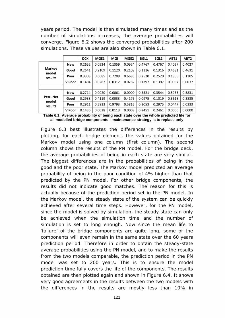
121
years period. The model is then simulated many times and as the
number of simulations increases, the average probabilities will
converge. Figure 6.2 shows the converged probabilities after 200
simulations. These values are also shown in Table 6.1.
DCK MGE1 MGI MGE2 BGL1 BGL2 ABT1 ABT2
Markov model results
New 0.2652 0.0924 0.1359 0.0924 0.4767 0.4767 0.4027 0.4027
Good 0.2641 0.2109 0.1120 0.2109 0.1316 0.1316 0.4631 0.4631
Poor 0.3303 0.6685 0.7209 0.6685 0.2520 0.2520 0.1305 0.1305
V Poor 0.1404 0.0282 0.0312 0.0282 0.1397 0.1397 0.0037 0.0037
Petri-Net model results
New 0.2714 0.0020 0.0061 0.0000 0.3521 0.3544 0.5935 0.5831
Good 0.2938 0.4119 0.0033 0.4176 0.0975 0.1019 0.3618 0.3835
Poor 0.2911 0.5833 0.9793 0.5816 0.3053 0.2975 0.0447 0.0333
V Poor 0.1436 0.0028 0.0113 0.0008 0.2451 0.2461 0.0000 0.0000
Table 6.1: Average probability of being each state over the whole predicted life for all modelled bridge components – maintenance strategy is to replace only
Figure 6.3 best illustrates the differences in the results by
plotting, for each bridge element, the values obtained for the
Markov model using one column (first column). The second
column shows the results of the PN model. For the bridge deck,
the average probabilities of being in each state are very similar.
The biggest differences are in the probabilities of being in the
good and the poor state. The Markov model predicted an average
probability of being in the poor condition of 4% higher than that
predicted by the PN model. For other bridge components, the
results did not indicate good matches. The reason for this is
actually because of the prediction period set in the PN model. In
the Markov model, the steady state of the system can be quickly
achieved after several time steps. However, for the PN model,
since the model is solved by simulation, the steady state can only
be achieved when the simulation time and the number of
simulation is set to long enough. Now since the mean life to
‘failure’ of the bridge components are quite long, some of the
components will even remain in the same state over the 60 years
prediction period. Therefore in order to obtain the steady-state
average probabilities using the PN model, and to make the results
from the two models comparable, the prediction period in the PN
model was set to 200 years. This is to ensure the model
prediction time fully covers the life of the components. The results
obtained are then plotted again and shown in Figure 6.4. It shows
very good agreements in the results between the two models with
the differences in the results are mostly less than 10% in
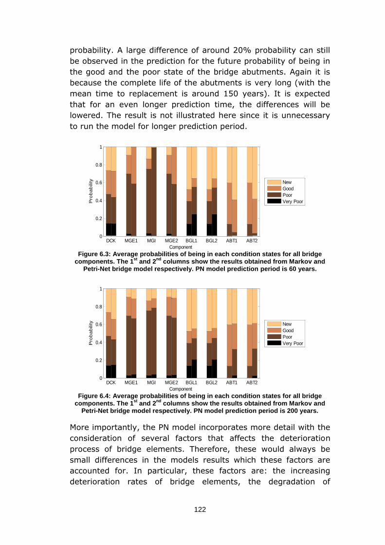
122
probability. A large difference of around 20% probability can still
be observed in the prediction for the future probability of being in
the good and the poor state of the bridge abutments. Again it is
because the complete life of the abutments is very long (with the
mean time to replacement is around 150 years). It is expected
that for an even longer prediction time, the differences will be
lowered. The result is not illustrated here since it is unnecessary
to run the model for longer prediction period.
Figure 6.3: Average probabilities of being in each condition states for all bridge
components. The 1st
and 2nd
columns show the results obtained from Markov and Petri-Net bridge model respectively. PN model prediction period is 60 years.
Figure 6.4: Average probabilities of being in each condition states for all bridge
components. The 1st
and 2nd
columns show the results obtained from Markov and Petri-Net bridge model respectively. PN model prediction period is 200 years.
More importantly, the PN model incorporates more detail with the
consideration of several factors that affects the deterioration
process of bridge elements. Therefore, these would always be
small differences in the models results which these factors are
accounted for. In particular, these factors are: the increasing
deterioration rates of bridge elements, the degradation of
DCK MGE1 MGI MGE2 BGL1 BGL2 ABT1 ABT20
0.2
0.4
0.6
0.8
1
Component
Pro
ba
bili
ty
New
Good
Poor
Very Poor
DCK MGE1 MGI MGE2 BGL1 BGL2 ABT1 ABT20
0.2
0.4
0.6
0.8
1
Component
Pro
ba
bili
ty
New
Good
Poor
Very Poor
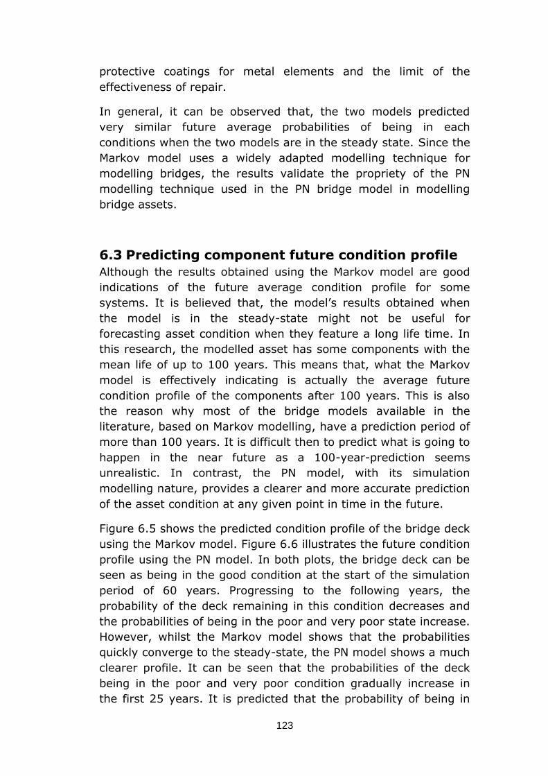
123
protective coatings for metal elements and the limit of the
effectiveness of repair.
In general, it can be observed that, the two models predicted
very similar future average probabilities of being in each
conditions when the two models are in the steady state. Since the
Markov model uses a widely adapted modelling technique for
modelling bridges, the results validate the propriety of the PN
modelling technique used in the PN bridge model in modelling
bridge assets.
6.3 Predicting component future condition profile
Although the results obtained using the Markov model are good
indications of the future average condition profile for some
systems. It is believed that, the model’s results obtained when
the model is in the steady-state might not be useful for
forecasting asset condition when they feature a long life time. In
this research, the modelled asset has some components with the
mean life of up to 100 years. This means that, what the Markov
model is effectively indicating is actually the average future
condition profile of the components after 100 years. This is also
the reason why most of the bridge models available in the
literature, based on Markov modelling, have a prediction period of
more than 100 years. It is difficult then to predict what is going to
happen in the near future as a 100-year-prediction seems
unrealistic. In contrast, the PN model, with its simulation
modelling nature, provides a clearer and more accurate prediction
of the asset condition at any given point in time in the future.
Figure 6.5 shows the predicted condition profile of the bridge deck
using the Markov model. Figure 6.6 illustrates the future condition
profile using the PN model. In both plots, the bridge deck can be
seen as being in the good condition at the start of the simulation
period of 60 years. Progressing to the following years, the
probability of the deck remaining in this condition decreases and
the probabilities of being in the poor and very poor state increase.
However, whilst the Markov model shows that the probabilities
quickly converge to the steady-state, the PN model shows a much
clearer profile. It can be seen that the probabilities of the deck
being in the poor and very poor condition gradually increase in
the first 25 years. It is predicted that the probability of being in
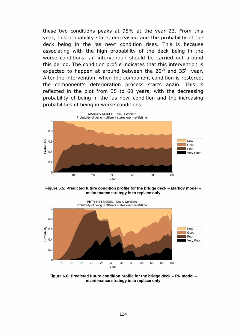
124
these two conditions peaks at 95% at the year 23. From this
year, this probability starts decreasing and the probability of the
deck being in the ‘as new’ condition rises. This is because
associating with the high probability of the deck being in the
worse conditions, an intervention should be carried out around
this period. The condition profile indicates that this intervention is
expected to happen at around between the 20th and 35th year.
After the intervention, when the component condition is restored,
the component’s deterioration process starts again. This is
reflected in the plot from 35 to 60 years, with the decreasing
probability of being in the ‘as new’ condition and the increasing
probabilities of being in worse conditions.
Figure 6.5: Predicted future condition profile for the bridge deck – Markov model – maintenance strategy is to replace only
Figure 6.6: Predicted future condition profile for the bridge deck – PN model – maintenance strategy is to replace only
0 10 20 30 40 50 600
0.2
0.4
0.6
0.8
1
Year
Pro
ba
bili
ty
MARKOV MODEL - Deck, ConcreteProbability of being in different states over the lifetime
New
Good
Poor
Very Poor
5 10 15 20 25 30 35 40 45 50 55 600
0.2
0.4
0.6
0.8
1
Year
Pro
ba
bili
ty
PETRI-NET MODEL - Deck, ConcreteProbability of being in different states over the lifetime
New
Good
Poor
Very Poor
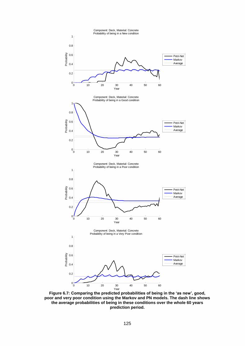
125
Figure 6.7: Comparing the predicted probabilities of being in the ‘as new’, good,
poor and very poor condition using the Markov and PN models. The dash line shows the average probabilities of being in these conditions over the whole 60 years
prediction period.
0 10 20 30 40 50 600
0.2
0.4
0.6
0.8
1
Year
Pro
ba
bili
ty
Component: Deck, Material: ConcreteProbability of being in a New condition
Petri-Net
Markov
Average
0 10 20 30 40 50 600
0.2
0.4
0.6
0.8
1
Year
Pro
ba
bili
ty
Component: Deck, Material: ConcreteProbability of being in a Good condition
Petri-Net
Markov
Average
0 10 20 30 40 50 600
0.2
0.4
0.6
0.8
1
Year
Pro
ba
bili
ty
Component: Deck, Material: ConcreteProbability of being in a Poor condition
Petri-Net
Markov
Average
0 10 20 30 40 50 600
0.2
0.4
0.6
0.8
1
Year
Pro
ba
bili
ty
Component: Deck, Material: ConcreteProbability of being in a Very Poor condition
Petri-Net
Markov
Average
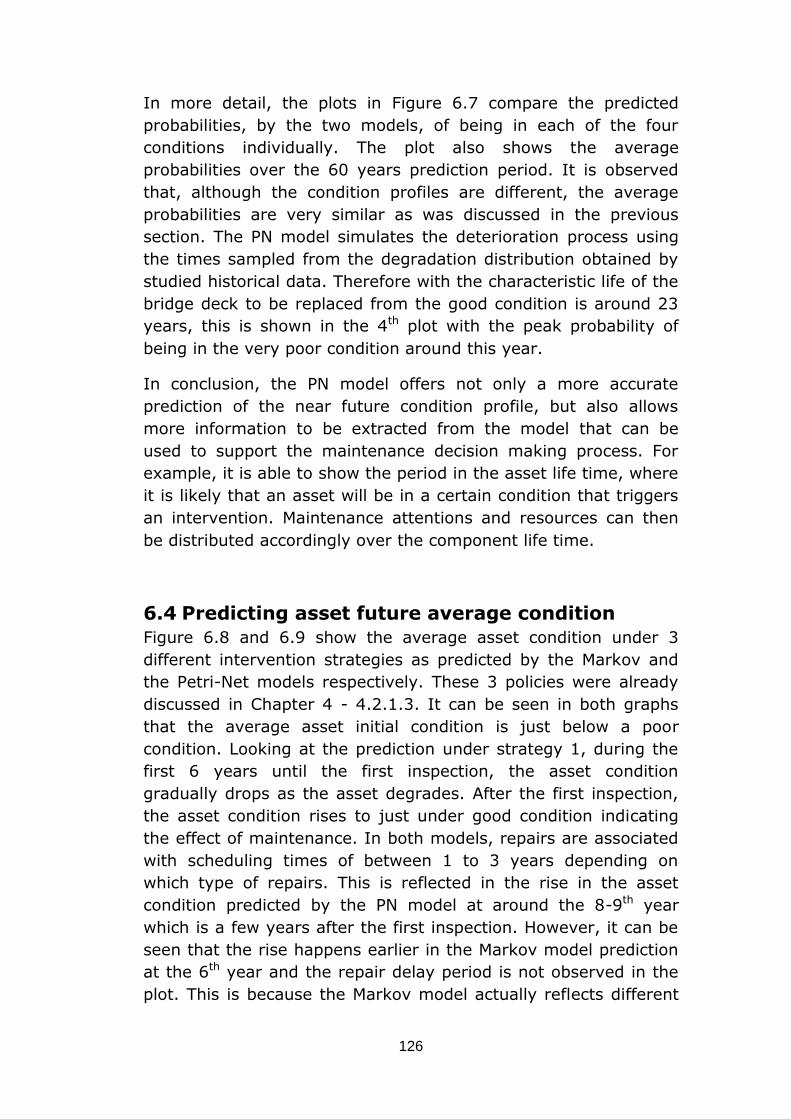
126
In more detail, the plots in Figure 6.7 compare the predicted
probabilities, by the two models, of being in each of the four
conditions individually. The plot also shows the average
probabilities over the 60 years prediction period. It is observed
that, although the condition profiles are different, the average
probabilities are very similar as was discussed in the previous
section. The PN model simulates the deterioration process using
the times sampled from the degradation distribution obtained by
studied historical data. Therefore with the characteristic life of the
bridge deck to be replaced from the good condition is around 23
years, this is shown in the 4th plot with the peak probability of
being in the very poor condition around this year.
In conclusion, the PN model offers not only a more accurate
prediction of the near future condition profile, but also allows
more information to be extracted from the model that can be
used to support the maintenance decision making process. For
example, it is able to show the period in the asset life time, where
it is likely that an asset will be in a certain condition that triggers
an intervention. Maintenance attentions and resources can then
be distributed accordingly over the component life time.
6.4 Predicting asset future average condition
Figure 6.8 and 6.9 show the average asset condition under 3
different intervention strategies as predicted by the Markov and
the Petri-Net models respectively. These 3 policies were already
discussed in Chapter 4 - 4.2.1.3. It can be seen in both graphs
that the average asset initial condition is just below a poor
condition. Looking at the prediction under strategy 1, during the
first 6 years until the first inspection, the asset condition
gradually drops as the asset degrades. After the first inspection,
the asset condition rises to just under good condition indicating
the effect of maintenance. In both models, repairs are associated
with scheduling times of between 1 to 3 years depending on
which type of repairs. This is reflected in the rise in the asset
condition predicted by the PN model at around the 8-9th year
which is a few years after the first inspection. However, it can be
seen that the rise happens earlier in the Markov model prediction
at the 6th year and the repair delay period is not observed in the
plot. This is because the Markov model actually reflects different
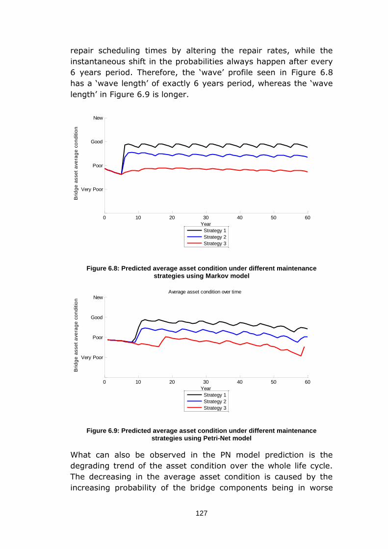
127
repair scheduling times by altering the repair rates, while the
instantaneous shift in the probabilities always happen after every
6 years period. Therefore, the ‘wave’ profile seen in Figure 6.8
has a ‘wave length’ of exactly 6 years period, whereas the ‘wave
length’ in Figure 6.9 is longer.
Figure 6.8: Predicted average asset condition under different maintenance strategies using Markov model
Figure 6.9: Predicted average asset condition under different maintenance strategies using Petri-Net model
What can also be observed in the PN model prediction is the
degrading trend of the asset condition over the whole life cycle.
The decreasing in the average asset condition is caused by the
increasing probability of the bridge components being in worse
0 10 20 30 40 50 60
Very Poor
Poor
Good
New
Year
Bri
dg
e a
sse
t a
ve
rag
e c
on
ditio
n
Strategy 1
Strategy 2
Strategy 3
0 10 20 30 40 50 60
Very Poor
Poor
Good
New
Year
Bri
dg
e a
sse
t a
ve
rag
e c
on
ditio
n
Average asset condition over time
Strategy 1
Strategy 2
Strategy 3
128
states as the prediction time progresses. In both models, the
repair is assumed to be perfect i.e. the condition of the
component is restored to ‘as good as new’ at repair. This means
that for strategy 1 and 2, as long as the inspection is carried out
frequently enough so that minor and major interventions can be
carried out before the component reaches the very poor state, the
component will never have to be replaced. This is implied in the
Markov model prediction as strategy 1 and 2 would maintain the
asset condition at a constant condition level. In the PN model, the
introduction of a limit to the number of effective repairs means
that once the number minor and major interventions has been
reached, the component has no choice but to degrade to the very
poor state where it is renewed. This results in an increase of the
probability of the components being in worse states as the
number of interventions (minor and major repair) increases,
hence the asset average condition gradually declines.
Strategy 3 allows the component to deteriorate until complete
replacement. Because different components have different times
to degrade which are, in many cases, longer than 60 years
prediction period, some components would be replaced whilst
other components are still degrading to the very poor state. Since
the average asset condition is calculated as the average of all
component conditions, the degradation of one component would
also reflect in the degradation of the whole asset condition.
Therefore, the degrading trend of the asset under this strategy
can be seen in both models.
6.5 Predicting maintenance cost
Table 6.2 contains the predicted whole life cycle costs (WLCC) for
each of the modelled bridge elements under three different
intervention strategies. As discussed earlier, with the Markov
model having constant deterioration rates, it doesn’t account for
the wear out effects of bridge components as does the PN model.
Thus the Markov model tends to underestimate the probabilities
of the bridge components being in worse states (poor and very
poor state), this results in a slightly smaller estimations of the
WLCC predicted by the Markov model comparing with the PN
model for strategy 2 and 3. The underestimation of the
probabilities being in the worse states means that the Markov
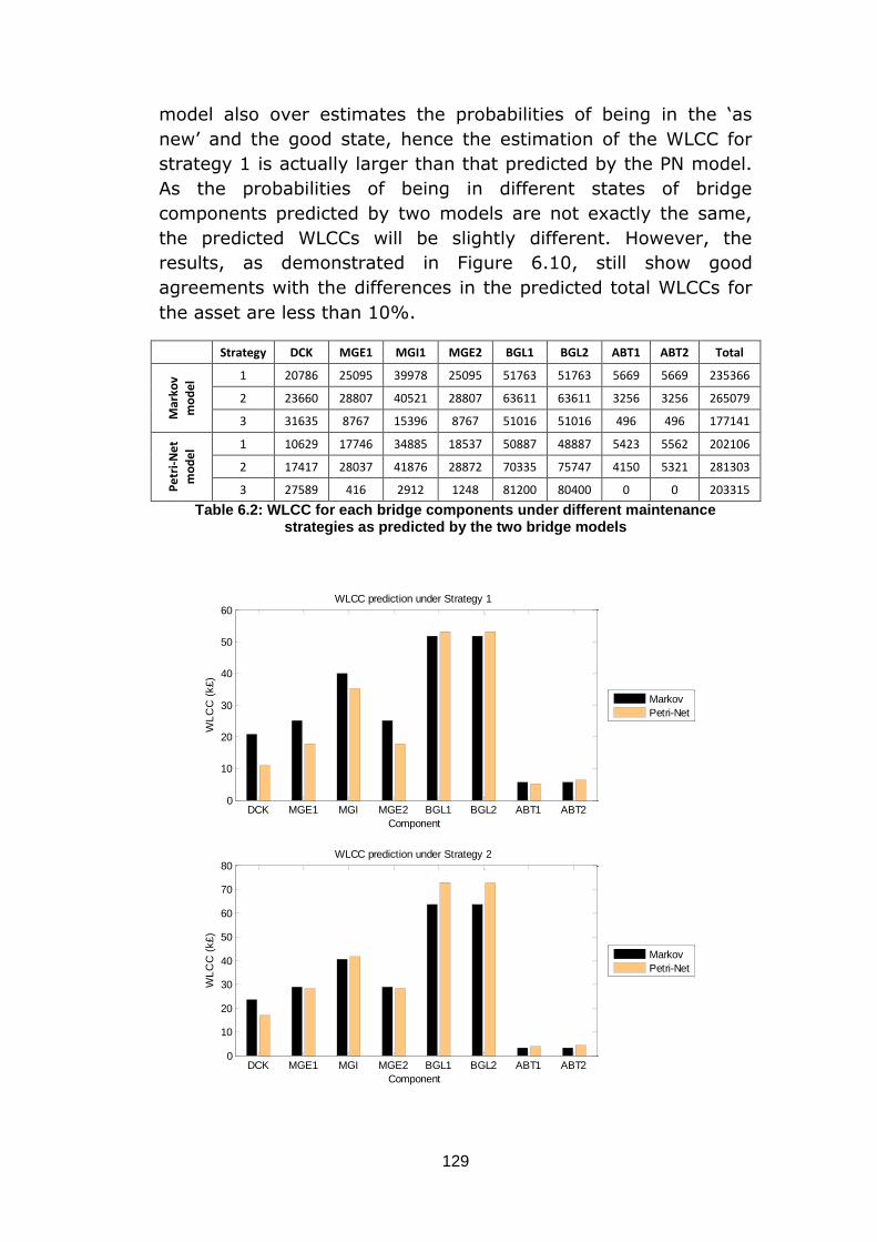
129
model also over estimates the probabilities of being in the ‘as
new’ and the good state, hence the estimation of the WLCC for
strategy 1 is actually larger than that predicted by the PN model.
As the probabilities of being in different states of bridge
components predicted by two models are not exactly the same,
the predicted WLCCs will be slightly different. However, the
results, as demonstrated in Figure 6.10, still show good
agreements with the differences in the predicted total WLCCs for
the asset are less than 10%.
Strategy DCK MGE1 MGI1 MGE2 BGL1 BGL2 ABT1 ABT2 Total
Mar
kov
mo
de
l 1 20786 25095 39978 25095 51763 51763 5669 5669 235366
2 23660 28807 40521 28807 63611 63611 3256 3256 265079
3 31635 8767 15396 8767 51016 51016 496 496 177141
Pe
tri-
Ne
t
mo
de
l 1 10629 17746 34885 18537 50887 48887 5423 5562 202106
2 17417 28037 41876 28872 70335 75747 4150 5321 281303
3 27589 416 2912 1248 81200 80400 0 0 203315
Table 6.2: WLCC for each bridge components under different maintenance strategies as predicted by the two bridge models
DCK MGE1 MGI MGE2 BGL1 BGL2 ABT1 ABT20
10
20
30
40
50
60
Component
WL
CC
(k£
)
WLCC prediction under Strategy 1
Markov
Petri-Net
DCK MGE1 MGI MGE2 BGL1 BGL2 ABT1 ABT20
10
20
30
40
50
60
70
80
Component
WL
CC
(k£
)
WLCC prediction under Strategy 2
Markov
Petri-Net
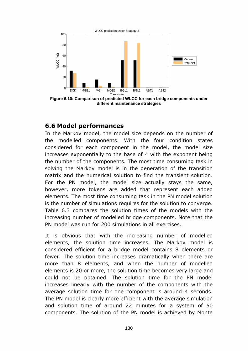
130
Figure 6.10: Comparison of predicted WLCC for each bridge components under
different maintenance strategies
6.6 Model performances
In the Markov model, the model size depends on the number of
the modelled components. With the four condition states
considered for each component in the model, the model size
increases exponentially to the base of 4 with the exponent being
the number of the components. The most time consuming task in
solving the Markov model is in the generation of the transition
matrix and the numerical solution to find the transient solution.
For the PN model, the model size actually stays the same,
however, more tokens are added that represent each added
elements. The most time consuming task in the PN model solution
is the number of simulations requires for the solution to converge.
Table 6.3 compares the solution times of the models with the
increasing number of modelled bridge components. Note that the
PN model was run for 200 simulations in all exercises.
It is obvious that with the increasing number of modelled
elements, the solution time increases. The Markov model is
considered efficient for a bridge model contains 8 elements or
fewer. The solution time increases dramatically when there are
more than 8 elements, and when the number of modelled
elements is 20 or more, the solution time becomes very large and
could not be obtained. The solution time for the PN model
increases linearly with the number of the components with the
average solution time for one component is around 4 seconds.
The PN model is clearly more efficient with the average simulation
and solution time of around 22 minutes for a system of 50
components. The solution of the PN model is achieved by Monte
DCK MGE1 MGI MGE2 BGL1 BGL2 ABT1 ABT20
20
40
60
80
100
Component
WL
CC
(k£
)
WLCC prediction under Strategy 3
Markov
Petri-Net
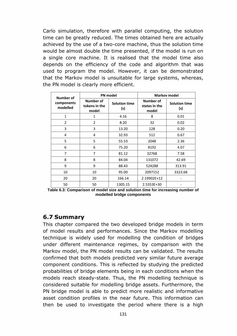
131
Carlo simulation, therefore with parallel computing, the solution
time can be greatly reduced. The times obtained here are actually
achieved by the use of a two-core machine, thus the solution time
would be almost double the time presented, if the model is run on
a single core machine. It is realised that the model time also
depends on the efficiency of the code and algorithm that was
used to program the model. However, it can be demonstrated
that the Markov model is unsuitable for large systems, whereas,
the PN model is clearly more efficient.
Number of components
modelled
PN model Markov model
Number of tokens in the
model
Solution time (s)
Number of states in the
model
Solution time (s)
1 1 4.16 8 0.01
2 2 8.20 32 0.02
3 3 13.20 128 0.20
4 4 32.93 512 0.67
5 5 55.53 2048 2.36
6 6 75.20 8192 4.07
7 7 81.12 32768 7.58
8 8 84.04 131072 42.69
9 9 88.43 524288 313.91
10 10 95.00 2097152 3323.68
20 20 166.14 2.19902E+12 -
50 50 1305.15 2.5353E+30 -
Table 6.3: Comparison of model size and solution time for increasing number of modelled bridge components
6.7 Summary
This chapter compared the two developed bridge models in term
of model results and performances. Since the Markov modelling
technique is widely used for modelling the condition of bridges
under different maintenance regimes, by comparison with the
Markov model, the PN model results can be validated. The results
confirmed that both models predicted very similar future average
component conditions. This is reflected by studying the predicted
probabilities of bridge elements being in each conditions when the
models reach steady-state. Thus, the PN modelling technique is
considered suitable for modelling bridge assets. Furthermore, the
PN bridge model is able to predict more realistic and informative
asset condition profiles in the near future. This information can
then be used to investigate the period where there is a high

132
probability of an asset being in a poor or a very poor condition,
thus maintenance and inspection can be focused accordingly.
It is also demonstrated that, whilst the Markov model is efficient
for small bridge systems, an increase in the number of
components considered in the model has a considerable effect on
the number of resulting states which significantly increases the
solution time. The PN model is more efficient in the modelling
time especially with a system contains of many components.
Moreover, the nature of the PN model lends itself to parallel
computing enabling the simulation time can be decreased using
high performance computing.
133
Chapter 7 - Bridge Maintenance Optimisation
7.1 Introduction
An important use for models of engineering systems is to
establish the parameters which can be selected in order to deliver
the ‘best’ or optimal performance. In particular, for asset
management, is the desire to find the best maintenance strategy
that would result in the lowest whole life cycle cost or the best
asset condition so the risk of service disruption is minimised. The
easiest way to find the optimum solution is by exhaustive search.
This involves evaluating all possible candidate solutions to find the
fittest one. However, most engineering problems are complex in
which case the evaluation of each potential solution is a time
consuming task. This is especially true if, in addition, there is a
large dimensioned search space. These factors prohibit the option
to try each solution one by one. Therefore, an optimisation
technique is employed in finding the best solutions. The
optimisation technique used in this project is the Genetic
Algorithms (GA). This technique is chosen because: it is a flexible
method capable of solving a wide range of optimisation problems
with a diversity of variable and constraint types. The GA is also
used because it is a simple concept based on the natural
evolution and is easy to understand and apply. Also the
interaction between variables in this problem is low so the GA is
suitable (Haupt and Haupt, 2004).
134
7.1.1 Genetic Algorithm optimisation
The Genetic Algorithm (GA), first conceived by Holland (1975), is
an optimisation and search technique based on the principles of
genetics and natural evolution. Based on Darwin’s survival-of-the-
fittest principles, the GA’s intelligent search procedures find the
best and fittest design solutions which are otherwise difficult to
find using other techniques. The GA is considered one of the most
powerful search and optimization algorithms because the GA is
conducted using a population of points rather than a single point,
thus increasing the exploratory capability of the GA (Samhouri,
2009). In addition, the GA lends itself naturally to implementation
in parallel processing, with the potential to achieve faster
computational times. The GA works with a direct coding of the
parameter set rather than the parameters themselves, so, it is
suitable for discontinuous, high dimensional and multi-nodal
problems. Overall, the advantages of the GA (Haupt and Haupt,
2004) include:
Optimising with either continuous or discrete variables,
Doesn’t require derivative information of the objective
functions,
Deals with complex problems of a large number of
variables,
Well suited for parallel computers hence potential faster
solution times,
Produces a set of optimum solutions, not just one
optimum solution,
Technique that can be easily adapted to a wide range of
problems in all fields.
There are seven important steps in the GA optimisation process
(coding & decoding, initial population generation, fitness function
evaluation, selection, mating and mutation) illustrated in Figure
7.1. At the start of the process, the variables to be optimised and
the objective functions must be defined. The objective functions
are dependent upon the variables and are used to measure if one
solution is better than another. In GA terms, the objective
function generates the ‘fitness’ of an ‘individual’. The next step is
generating the initial population where the variable value
representing each individual in the population is encoded by a
binary string. From this population, the fitness of each individual
is evaluated. These individuals are then ranked according to their
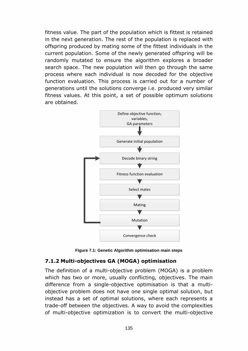
135
fitness value. The part of the population which is fittest is retained
in the next generation. The rest of the population is replaced with
offspring produced by mating some of the fittest individuals in the
current population. Some of the newly generated offspring will be
randomly mutated to ensure the algorithm explores a broader
search space. The new population will then go through the same
process where each individual is now decoded for the objective
function evaluation. This process is carried out for a number of
generations until the solutions converge i.e. produced very similar
fitness values. At this point, a set of possible optimum solutions
are obtained.
Figure 7.1: Genetic Algorithm optimisation main steps
7.1.2 Multi-objectives GA (MOGA) optimisation
The definition of a multi-objective problem (MOGA) is a problem
which has two or more, usually conflicting, objectives. The main
difference from a single-objective optimisation is that a multi-
objective problem does not have one single optimal solution, but
instead has a set of optimal solutions, where each represents a
trade-off between the objectives. A way to avoid the complexities
of multi-objective optimization is to convert the multi-objective
Define objective function, variables,
GA parameters
Generate initial population
Decode binary string
Fitness function evaluation
Select mates
Mating
Mutation
Convergence check

136
problem into a single-objective problem by assigning weights to
the different objectives and then calculating a single fitness value.
The major problem with this weighted sum approach is that it is
subjective, as it ultimately leaves it to the decision maker to
assign weights according to the subjective importance of the
corresponding objectives.
For the modelling purposes of this project, it is of interest to
optimise a number of objectives at the same time. A single
optimisation exercise was actually applied to find the maintenance
policies that result in the lowest life cycle cost (LCC). It was found
that, the optimisation usually looks for the strategy that carries
out the least number of interventions in order to achieve
minimum LCC. This could be undesirable in some cases since
these optimum policies, which carry out ‘minimum’ work, means
that the asset condition would be around the critical condition
over its life. Moreover, it is believed that the solutions only cover
the extreme part of the solution space which might not be
meaningful in aiding the maintenance decision making process.
Therefore, two objectives are chosen for the optimisation problem
in this research which are the asset life cycle cost and the asset
average condition. The optimisation exercise is then to find the
optimum maintenance strategy that gives the lowest LCC whilst
maximising the condition of an asset. The MOGA ranks these
objectives according to the Pareto front. The ranking will be
discussed in more details later on.
7.1.3 Optimisation procedure
There are two bridge models have been developed in this
research, based on the Markov and Petri-net method. These two
bridge models will be optimised separately and the optimisation
process implementation for each model will be discussed in detail.
The next sections discuss the optimisation of the Markov and
Petri-net bridge models. It is worth noting that, the optimisation
of the PN model is a hybrid optimisation, i.e. the results from the
optimisation of the Markov model are used as the initial starting
points for the PN model optimisation resulting in a performance
increase.
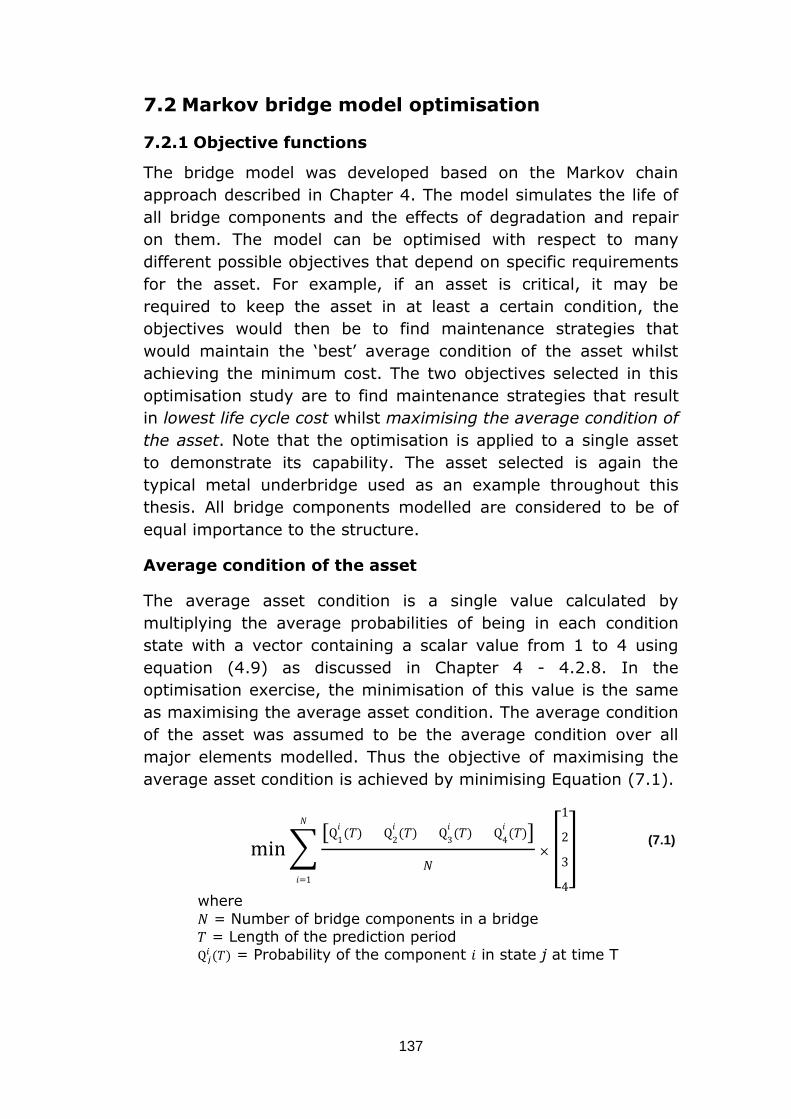
137
7.2 Markov bridge model optimisation
7.2.1 Objective functions
The bridge model was developed based on the Markov chain
approach described in Chapter 4. The model simulates the life of
all bridge components and the effects of degradation and repair
on them. The model can be optimised with respect to many
different possible objectives that depend on specific requirements
for the asset. For example, if an asset is critical, it may be
required to keep the asset in at least a certain condition, the
objectives would then be to find maintenance strategies that
would maintain the ‘best’ average condition of the asset whilst
achieving the minimum cost. The two objectives selected in this
optimisation study are to find maintenance strategies that result
in lowest life cycle cost whilst maximising the average condition of
the asset. Note that the optimisation is applied to a single asset
to demonstrate its capability. The asset selected is again the
typical metal underbridge used as an example throughout this
thesis. All bridge components modelled are considered to be of
equal importance to the structure.
Average condition of the asset
The average asset condition is a single value calculated by
multiplying the average probabilities of being in each condition
state with a vector containing a scalar value from 1 to 4 using
equation (4.9) as discussed in Chapter 4 - 4.2.8. In the
optimisation exercise, the minimisation of this value is the same
as maximising the average asset condition. The average condition
of the asset was assumed to be the average condition over all
major elements modelled. Thus the objective of maximising the
average asset condition is achieved by minimising Equation (7.1).
∑
( )
( )
( )
( )
[
] (7.1)
where
= Number of bridge components in a bridge
= Length of the prediction period
( ) = Probability of the component in state j at time T
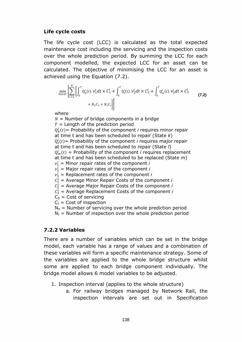
138
Life cycle costs
The life cycle cost (LCC) is calculated as the total expected
maintenance cost including the servicing and the inspection costs
over the whole prediction period. By summing the LCC for each
component modelled, the expected LCC for an asset can be
calculated. The objective of minimising the LCC for an asset is
achieved using the Equation (7.2).
[∑ [∫ ( )
∫
( )
∫ ( )
]]
(7.2)
where
= Number of bridge components in a bridge
= Length of the prediction period
( )= Probability of the component i requires minor repair
at time t and has been scheduled to repair (State k)
( )= Probability of the component i requires major repair
at time t and has been scheduled to repair (State l)
( ) = Probability of the component i requires replacement
at time t and has been scheduled to be replaced (State m)
= Minor repair rates of the component i
= Major repair rates of the component i
= Replacement rates of the component i
= Average Minor Repair Costs of the component i
= Average Major Repair Costs of the component i
= Average Replacement Costs of the component i
CS = Cost of servicing CI = Cost of inspection NS = Number of servicing over the whole prediction period NI = Number of inspection over the whole prediction period
7.2.2 Variables
There are a number of variables which can be set in the bridge
model, each variable has a range of values and a combination of
these variables will form a specific maintenance strategy. Some of
the variables are applied to the whole bridge structure whilst
some are applied to each bridge component individually. The
bridge model allows 6 model variables to be adjusted.
1. Inspection interval (applies to the whole structure)
a. For railway bridges managed by Network Rail, the
inspection intervals are set out in Specification
139
NR/SP/CIV/017 (Network Rail, 2004a). 16 potential
intervals were chosen, ranging between 1 to 16 years.
2. Opportunistic maintenance (applies to the whole structure)
a. Opportunistic maintenance can be enabled or disabled
for an asset.
3. Intervention options (applies to individual elements)
a. Option 1: Intervene at good condition – repair as
soon as any component is revealed to be in any
degraded state (good or worse).
b. Option 2: Intervene at poor condition – carry out
major repair when the component reaches the poor
state.
c. Option 3: Intervene at very poor condition – only
perform renewals when the component reaches the
very poor state.
4. Servicing interval (applies to individual elements)
a. The servicing intervals considered in practice are set
in (RT/CE/C/002, 2002). 16 possible servicing
intervals were chosen, from 1 to 16 years.
5. Minor repair delay time (applies to individual elements)
a. In practice, Network Rail schedule interventions
according to a prioritised work bank and subject to
budget constraint. In additional, the design,
preparation and management time also contribute to
the delay time. It has been reported by bridge experts
that the delay time depends on the type of work and
can be up to 4 years (Halcrow, 2011). It was
suggested that it is reasonable to assume that minor
interventions can be delayed up to 2 years. Four
possible values were chosen: 6, 12, 18 and 24
months.
6. Major repair delay time (applies to individual elements)
a. It was also suggested by bridge experts that major
intervention can also be delayed up to 2 years, thus
four possible values were chosen: 6, 12, 24 and 36
months.
7. Renewal delay time (applies to individual elements)
a. Eight possible delay times were chosen: 6, 12, 18, 24,
30, 36, 42 and 48 months.
Table 7.1 summarises all the possible values which the variables
can take. Note that the inspection intervals and opportunistic

140
maintenance are set for the whole bridge structure, while other
variables can be set for each bridge components individually.
7.2.3 Variable encoding and decoding
The GA often uses binary to represent the variable values, this
process is called the variable encoding. Each variable is
represented by a string of bits, a bit can take a value of 0 or 1,
depending on the range of possible values that a particular
variable can take, an appropriate number of bits is required. The
binary strings representing each variable are then listed
contiguously to form an individual that represents a unique
possible maintenance strategy. An example is given in Figure 7.2
of the encoding process for three variables. Variable 1 can take
16 values so 4 bits string is used to represents these 24 = 16
options. Variable 2 can have 64 possible values so a string of 6
bits is used. Similarly, variable 3 uses a 3-bit string to represent 8
possible values. Thus, a string of total 13 bits long is used to
represent an individual.
⏞
⏟
⏞
⏟
⏞
⏟
Figure 7.2: Example of variable coding and decoding process
Variables Value
range Apply to
Number of
options for
the selected
variable
Number of bits
required to
represent
variable
selection Inspection
period
1:1:16
years
Asset 16 4
Opportunistic maintenance
0,1 (enabled, disabled)
Asset 2 1
Intervention options
1, 2, 3 Component 3 2
Servicing interval
1:1:16 years
Component 16 4
Minor repair
delay time
6,12,18,24
months
Component 4 2
Major repair delay time
6,12,24,36 months
Component 4 2
Renewal delay
time
6:6:48
months
Component 8 3
Table 7.1: Model variables and their value range
For the range of variable values shown in Table 7.1, firstly, a 13-
bit string (Figure 7.3) is used to code all the variables that apply
to a bridge component. Secondly, by combining these coded
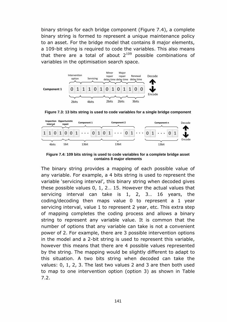
141
binary strings for each bridge component (Figure 7.4), a complete
binary string is formed to represent a unique maintenance policy
to an asset. For the bridge model that contains 8 major elements,
a 109-bit string is required to code the variables. This also means
that there are a total of about 2109 possible combinations of
variables in the optimisation search space.
ServicingServicingIntervention
option
Intervention option
0 1
2bits2bits 4bits4bits
1 1 0 1
Minor repair
delay time
Minor repair
delay time
Major repair
delay time
Major repair
delay timeRenewal
delay time
Renewal delay time
0 1 0 1 1 0
2bits2bits 2bits2bits 3bits3bits
0
Decode
Encode
Component 1Component 1
Figure 7.3: 13 bits string is used to code variables for a single bridge component
Opportunistic repair
Opportunistic repair
1bit1bit
0
Inspection interval
Inspection interval
1 1 0 1
4bits4bits
0 1 0 1. . .
13bit13bit
Component 1Component 1
0 1 0 1. . .
13bit13bit
Component 2Component 2
. . . 0 1 0 1. . .
13bit13bit
Component nComponent n Decode
Encode
Figure 7.4: 109 bits string is used to code variables for a complete bridge asset contains 8 major elements
The binary string provides a mapping of each possible value of
any variable. For example, a 4 bits string is used to represent the
variable ‘servicing interval’, this binary string when decoded gives
these possible values 0, 1, 2… 15. However the actual values that
servicing interval can take is 1, 2, 3… 16 years, the
coding/decoding then maps value 0 to represent a 1 year
servicing interval, value 1 to represent 2 year, etc. This extra step
of mapping completes the coding process and allows a binary
string to represent any variable value. It is common that the
number of options that any variable can take is not a convenient
power of 2. For example, there are 3 possible intervention options
in the model and a 2-bit string is used to represent this variable,
however this means that there are 4 possible values represented
by the string. The mapping would be slightly different to adapt to
this situation. A two bits string when decoded can take the
values: 0, 1, 2, 3. The last two values 2 and 3 are then both used
to map to one intervention option (option 3) as shown in Table
7.2.
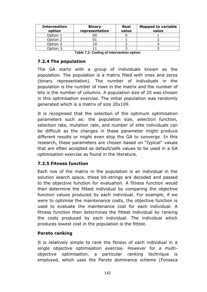
142
Intervention
option
Binary
representation
Real
value
Mapped to variable
value
Option 1 00 0 1
Option 2 01 1 2
Option 3 10 2 3
Option 3 11 3 3 Table 7.2: Coding of intervention option
7.2.4 The population
The GA starts with a group of individuals known as the
population. The population is a matrix filled with ones and zeros
(binary representation). The number of individuals in the
population is the number of rows in the matrix and the number of
bits is the number of columns. A population size of 20 was chosen
in this optimisation exercise. The initial population was randomly
generated which is a matrix of size 20x109.
It is recognised that the selection of the optimum optimisation
parameters such as: the population size, selection function,
selection rate, mutation rate, and number of elite individuals can
be difficult as the changes in these parameter might produce
different results or might even stop the GA to converge. In this
research, these parameters are chosen based on “typical” values
that are often accepted as default/safe values to be used in a GA
optimisation exercise as found in the literature.
7.2.5 Fitness function
Each row of the matrix in the population is an individual in the
solution search space, these bit-strings are decoded and passed
to the objective function for evaluation. A fitness function would
then determine the fittest individual by comparing the objective
function values produced by each individual. For example, if we
were to optimise the maintenance costs, the objective function is
used to evaluate the maintenance cost for each individual. A
fitness function then determines the fittest individual by ranking
the costs produced by each individual. The individual which
produces lowest cost in the population is the fittest.
Pareto ranking
It is relatively simple to rank the fitness of each individual in a
single objective optimisation exercise. However for a multi-
objective optimisation, a particular ranking technique is
employed, which uses the Pareto dominance scheme (Fonseca
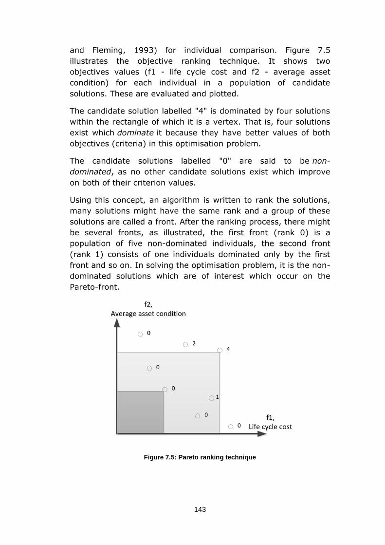
143
and Fleming, 1993) for individual comparison. Figure 7.5
illustrates the objective ranking technique. It shows two
objectives values (f1 - life cycle cost and f2 - average asset
condition) for each individual in a population of candidate
solutions. These are evaluated and plotted.
The candidate solution labelled "4" is dominated by four solutions
within the rectangle of which it is a vertex. That is, four solutions
exist which dominate it because they have better values of both
objectives (criteria) in this optimisation problem.
The candidate solutions labelled "0" are said to be non-
dominated, as no other candidate solutions exist which improve
on both of their criterion values.
Using this concept, an algorithm is written to rank the solutions,
many solutions might have the same rank and a group of these
solutions are called a front. After the ranking process, there might
be several fronts, as illustrated, the first front (rank 0) is a
population of five non-dominated individuals, the second front
(rank 1) consists of one individuals dominated only by the first
front and so on. In solving the optimisation problem, it is the non-
dominated solutions which are of interest which occur on the
Pareto-front.
Figure 7.5: Pareto ranking technique
11
00
00
00
00
00
2244
f2,Average asset condition
f2,Average asset condition
f1,Life cycle cost
f1,Life cycle cost
144
Selection rates
A selection rate, Xrate, is the fraction of the population that survive
for the next step of mating. The rest are discarded to make room
for the new offspring. The selection rate decides how many
individuals to keep. If only a few are selected to the next
generation, this will limit the available genes in the offspring.
Keeping too many will allow a bad performer a chance to
contribute bad genes to the next generation. The selection rate
was set at 0.5 which means that when all individuals in the
population of 20 are ranked, the 10 fittest individuals are kept
giving 10 free spaces in the population to be filled in the next
step.
7.2.6 Paring (selection function)
Pairing or mating of individuals will create offspring and this
process is repeated until the free places in the population are
filled with the new offspring. There are many ways to pair
individuals, the most common is by random paring. Other
methods can be employed such as weighted paring (where the
chance of fittest individual being mated is higher than less-fit
individual), tournament selection (randomly pick a small subset of
individuals and the fittest of these will become a parent, this is
best for larger population size and does not require sorting).
The technique was used in this research is rank pairing (Haupt
and Haupt, 2004). In this approach, the individuals are selected
randomly according to a rank probability calculated according to
Equation (2.5).
∑
(7.3)
As an example, the 10 fittest individuals in a population are listed
in Table 7.3. Their fitness values are calculated and they are
ranked according to the Pareto-front. The rank probability for
each individual can then be calculated based on its position from
the top of the list. The last column shows the cumulative rank
probability.
A random number between zero and one is then generated, the
first individual with a cumulative probability that is greater than
the random number is selected for paring. For instance, if the
random number is r=0.5555, then since 0.4909<r<0.6182, thus
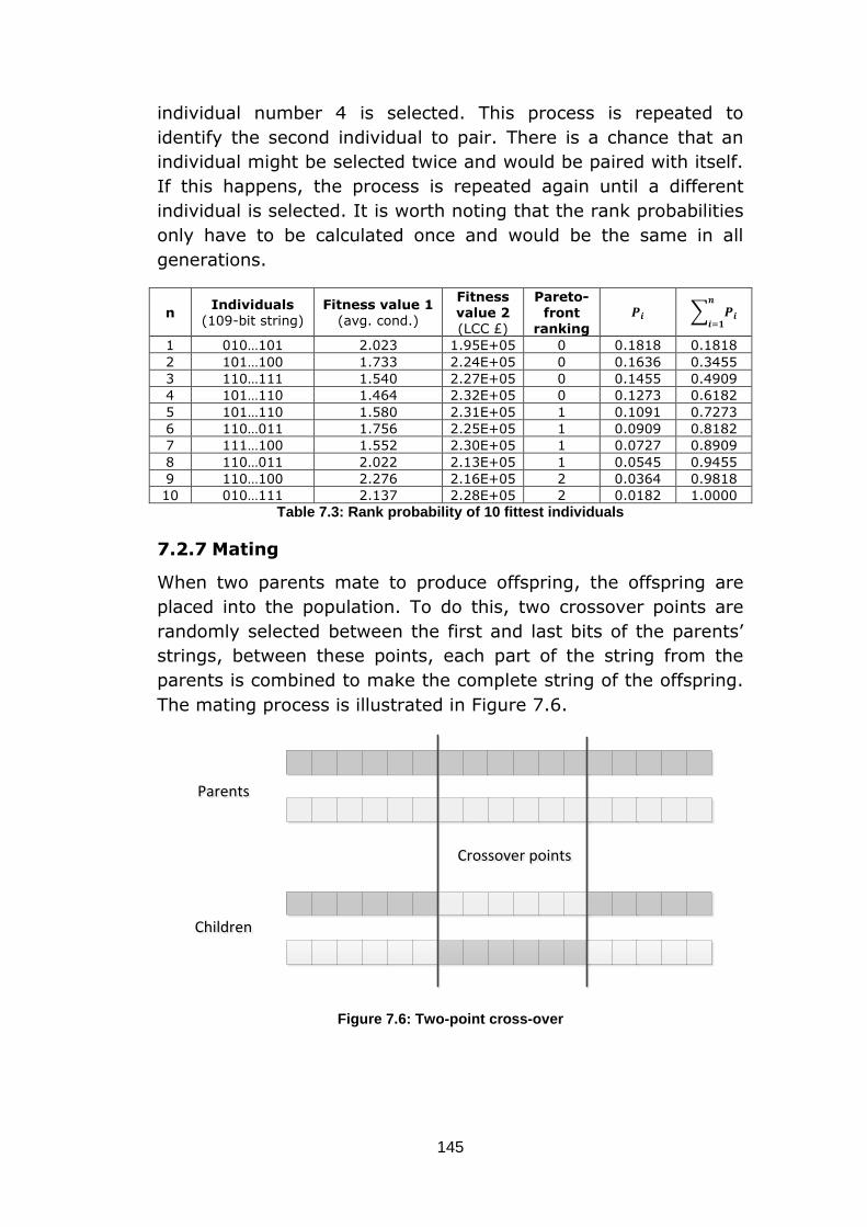
145
individual number 4 is selected. This process is repeated to
identify the second individual to pair. There is a chance that an
individual might be selected twice and would be paired with itself.
If this happens, the process is repeated again until a different
individual is selected. It is worth noting that the rank probabilities
only have to be calculated once and would be the same in all
generations.
n Individuals
(109-bit string) Fitness value 1
(avg. cond.)
Fitness value 2 (LCC £)
Pareto-front
ranking
∑
1 010…101 2.023 1.95E+05 0 0.1818 0.1818
2 101…100 1.733 2.24E+05 0 0.1636 0.3455
3 110…111 1.540 2.27E+05 0 0.1455 0.4909
4 101…110 1.464 2.32E+05 0 0.1273 0.6182
5 101…110 1.580 2.31E+05 1 0.1091 0.7273
6 110…011 1.756 2.25E+05 1 0.0909 0.8182
7 111…100 1.552 2.30E+05 1 0.0727 0.8909
8 110…011 2.022 2.13E+05 1 0.0545 0.9455
9 110…100 2.276 2.16E+05 2 0.0364 0.9818
10 010…111 2.137 2.28E+05 2 0.0182 1.0000
Table 7.3: Rank probability of 10 fittest individuals
7.2.7 Mating
When two parents mate to produce offspring, the offspring are
placed into the population. To do this, two crossover points are
randomly selected between the first and last bits of the parents’
strings, between these points, each part of the string from the
parents is combined to make the complete string of the offspring.
The mating process is illustrated in Figure 7.6.
Figure 7.6: Two-point cross-over
ParentsParents
ChildrenChildren
Crossover pointsCrossover points

146
7.2.8 Mutation
Random mutations alter a certain percentage of the bits in the
string. Mutation provides genetic diversity and allows the GA to
explore a broader space and prevent it from converging too fast
to a local optimal point before searching the entire space. A single
point mutation changes a bit from value 0 to 1 or vice versa. A
mutation rate can be set which indicates the number of bits will
be mutated in the population. In this optimisation, each individual
is a 109-bits string in a population size of 20. This would create a
population of 20x109=2180 bits. A mutation rate of 0.005 was
used, this means that 0.5% of the bits in the entire 2180 bits
population will be randomly mutated.
However, the problem with mutation is that it also mutates the
best solutions which can prevent the GA converging to the best
solutions. To prevent the mutation on the best solution, elitism is
introduced where a selection of fittest individuals are called elites.
An algorithm was developed so there are no mutations on these
elites and the first 5 fittest individuals in the population were set
as elite individuals.
7.2.9 Next generation and convergence
After the mutation, the objective functions are evaluated for the
offspring generated by the pairing, mating and mutation
processes. The process of pairing, mating and mutation is then
repeated again for the next population. This is repeated for a
number of generations which depends on whether the process has
converged. The convergence is considered when the values of the
objective function evaluations do not change from generation to
generation. In this work, the convergence is considered to be
achieved when all the individuals are in the top rank (rank 0 - the
first Pareto front).
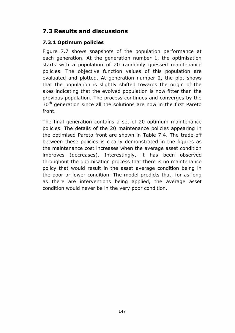
147
7.3 Results and discussions
7.3.1 Optimum policies
Figure 7.7 shows snapshots of the population performance at
each generation. At the generation number 1, the optimisation
starts with a population of 20 randomly guessed maintenance
policies. The objective function values of this population are
evaluated and plotted. At generation number 2, the plot shows
that the population is slightly shifted towards the origin of the
axes indicating that the evolved population is now fitter than the
previous population. The process continues and converges by the
30th generation since all the solutions are now in the first Pareto
front.
The final generation contains a set of 20 optimum maintenance
policies. The details of the 20 maintenance policies appearing in
the optimised Pareto front are shown in Table 7.4. The trade-off
between these policies is clearly demonstrated in the figures as
the maintenance cost increases when the average asset condition
improves (decreases). Interestingly, it has been observed
throughout the optimisation process that there is no maintenance
policy that would result in the asset average condition being in
the poor or lower condition. The model predicts that, for as long
as there are interventions being applied, the average asset
condition would never be in the very poor condition.
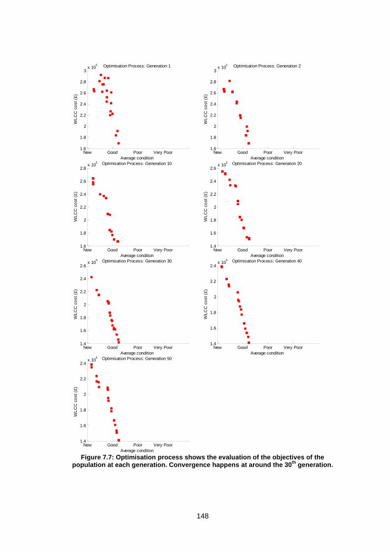
148
Figure 7.7: Optimisation process shows the evaluation of the objectives of the
population at each generation. Convergence happens at around the 30th
generation.
New Good Poor Very Poor1.6
1.8
2
2.2
2.4
2.6
2.8
3x 10
5
Average condition
WL
CC
co
st
(£)
Optimisation Process: Generation 1
New Good Poor Very Poor1.6
1.8
2
2.2
2.4
2.6
2.8
3x 10
5
Average condition
WL
CC
co
st
(£)
Optimisation Process: Generation 2
New Good Poor Very Poor1.6
1.8
2
2.2
2.4
2.6
2.8x 10
5
Average condition
WL
CC
co
st
(£)
Optimisation Process: Generation 10
New Good Poor Very Poor1.4
1.6
1.8
2
2.2
2.4
2.6x 10
5
Average condition
WL
CC
co
st
(£)
Optimisation Process: Generation 20
New Good Poor Very Poor1.4
1.6
1.8
2
2.2
2.4
2.6x 10
5
Average condition
WL
CC
co
st
(£)
Optimisation Process: Generation 30
New Good Poor Very Poor1.4
1.6
1.8
2
2.2
2.4x 10
5
Average condition
WL
CC
co
st
(£)
Optimisation Process: Generation 40
New Good Poor Very Poor1.4
1.6
1.8
2
2.2
2.4x 10
5
Average condition
WL
CC
co
st
(£)
Optimisation Process: Generation 50
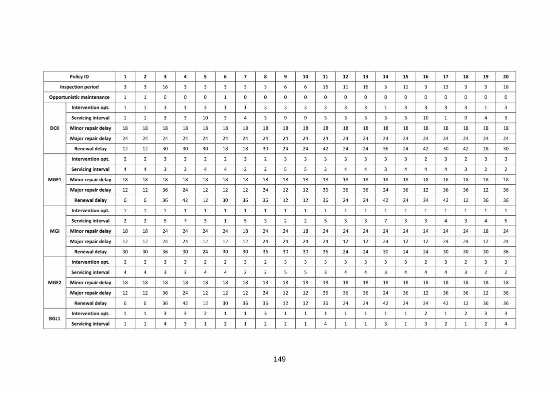
149
Policy ID 1 2 3 4 5 6 7 8 9 10 11 12 13 14 15 16 17 18 19 20
Inspection period 3 3 16 3 3 3 3 3 6 6 16 11 16 3 11 3 13 3 3 16
Opportunistic maintenance 1 1 0 0 0 1 0 0 0 0 0 0 0 0 0 0 0 0 0 0
DCK
Intervention opt. 1 1 3 1 3 1 1 3 3 3 3 3 3 1 3 3 3 3 1 3
Servicing interval 1 1 3 3 10 3 4 3 9 9 3 3 3 3 3 10 1 9 4 3
Minor repair delay 18 18 18 18 18 18 18 18 18 18 18 18 18 18 18 18 18 18 18 18
Major repair delay 24 24 24 24 24 24 24 24 24 24 24 24 24 24 24 24 24 24 24 24
Renewal delay 12 12 30 30 30 18 18 30 24 24 42 24 24 36 24 42 30 42 18 30
MGE1
Intervention opt. 2 2 3 3 2 2 3 2 3 3 3 3 3 3 3 2 3 2 3 3
Servicing interval 4 4 3 3 4 4 2 2 5 5 3 4 4 3 4 4 4 3 2 2
Minor repair delay 18 18 18 18 18 18 18 18 18 18 18 18 18 18 18 18 18 18 18 18
Major repair delay 12 12 36 24 12 12 12 24 12 12 36 36 36 24 36 12 36 36 12 36
Renewal delay 6 6 36 42 12 30 36 36 12 12 36 24 24 42 24 24 42 12 36 36
MGI
Intervention opt. 1 1 1 1 1 1 1 1 1 1 1 1 1 1 1 1 1 1 1 1
Servicing interval 2 2 5 7 3 1 5 3 2 2 5 3 3 7 3 3 4 3 4 5
Minor repair delay 18 18 24 24 24 24 18 24 24 18 24 24 24 24 24 24 24 24 18 24
Major repair delay 12 12 24 24 12 12 12 24 24 24 24 12 12 24 12 12 24 24 12 24
Renewal delay 30 30 36 30 24 30 30 36 30 30 36 24 24 30 24 24 30 30 30 36
MGE2
Intervention opt. 2 2 3 3 2 2 3 2 3 3 3 3 3 3 3 2 3 2 3 3
Servicing interval 4 4 3 3 4 4 2 2 5 5 3 4 4 3 4 4 4 3 2 2
Minor repair delay 18 18 18 18 18 18 18 18 18 18 18 18 18 18 18 18 18 18 18 18
Major repair delay 12 12 36 24 12 12 12 24 12 12 36 36 36 24 36 12 36 36 12 36
Renewal delay 6 6 36 42 12 30 36 36 12 12 36 24 24 42 24 24 42 12 36 36
BGL1 Intervention opt. 1 1 3 3 2 1 1 3 1 1 1 1 1 1 1 2 1 2 3 3
Servicing interval 1 1 4 3 1 2 1 2 2 1 4 1 1 3 1 3 2 1 2 4
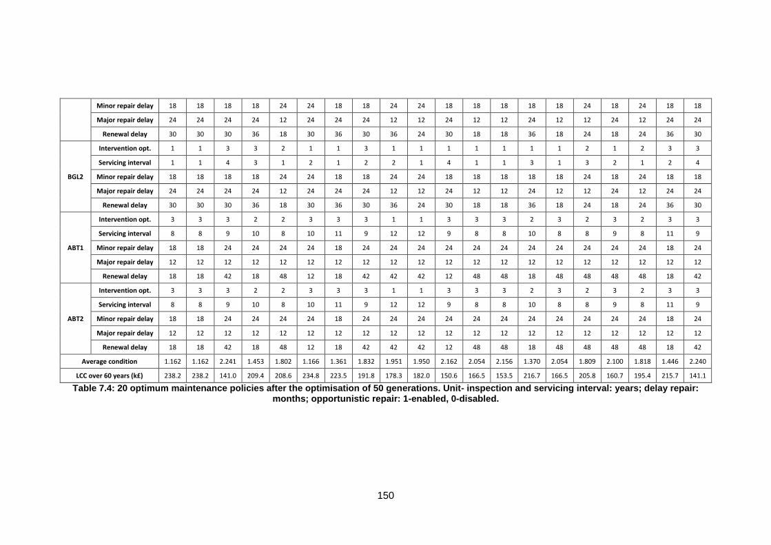
150
Minor repair delay 18 18 18 18 24 24 18 18 24 24 18 18 18 18 18 24 18 24 18 18
Major repair delay 24 24 24 24 12 24 24 24 12 12 24 12 12 24 12 12 24 12 24 24
Renewal delay 30 30 30 36 18 30 36 30 36 24 30 18 18 36 18 24 18 24 36 30
BGL2
Intervention opt. 1 1 3 3 2 1 1 3 1 1 1 1 1 1 1 2 1 2 3 3
Servicing interval 1 1 4 3 1 2 1 2 2 1 4 1 1 3 1 3 2 1 2 4
Minor repair delay 18 18 18 18 24 24 18 18 24 24 18 18 18 18 18 24 18 24 18 18
Major repair delay 24 24 24 24 12 24 24 24 12 12 24 12 12 24 12 12 24 12 24 24
Renewal delay 30 30 30 36 18 30 36 30 36 24 30 18 18 36 18 24 18 24 36 30
ABT1
Intervention opt. 3 3 3 2 2 3 3 3 1 1 3 3 3 2 3 2 3 2 3 3
Servicing interval 8 8 9 10 8 10 11 9 12 12 9 8 8 10 8 8 9 8 11 9
Minor repair delay 18 18 24 24 24 24 18 24 24 24 24 24 24 24 24 24 24 24 18 24
Major repair delay 12 12 12 12 12 12 12 12 12 12 12 12 12 12 12 12 12 12 12 12
Renewal delay 18 18 42 18 48 12 18 42 42 42 12 48 48 18 48 48 48 48 18 42
ABT2
Intervention opt. 3 3 3 2 2 3 3 3 1 1 3 3 3 2 3 2 3 2 3 3
Servicing interval 8 8 9 10 8 10 11 9 12 12 9 8 8 10 8 8 9 8 11 9
Minor repair delay 18 18 24 24 24 24 18 24 24 24 24 24 24 24 24 24 24 24 18 24
Major repair delay 12 12 12 12 12 12 12 12 12 12 12 12 12 12 12 12 12 12 12 12
Renewal delay 18 18 42 18 48 12 18 42 42 42 12 48 48 18 48 48 48 48 18 42
Average condition 1.162 1.162 2.241 1.453 1.802 1.166 1.361 1.832 1.951 1.950 2.162 2.054 2.156 1.370 2.054 1.809 2.100 1.818 1.446 2.240
LCC over 60 years (k£) 238.2 238.2 141.0 209.4 208.6 234.8 223.5 191.8 178.3 182.0 150.6 166.5 153.5 216.7 166.5 205.8 160.7 195.4 215.7 141.1
Table 7.4: 20 optimum maintenance policies after the optimisation of 50 generations. Unit- inspection and servicing interval: years; delay repair: months; opportunistic repair: 1-enabled, 0-disabled.

151
7.3.2 Comparison to industry maintenance policy
Policy Description
Standard This strategy is to intervene on bridges at a high level of tolerable
risk and to maintain the structures within a good condition state.
Minimum This strategy adopts a lower level of tolerable risk and accepts
elements within the bridge may be in good or poor condition.
Managed This strategy was developed to maintain current condition states
and assumes the lowest level of tolerable risk. Table 7.5: Maintenance policies employed by Network Rail (Halcrow, 2011)
Maintenance policies that are currently employed by Network Rail
on managing railway bridges are given in Table 7.5. Network Rail
has carried out case studies on a group of assets to determine the
optimum policies that would produce the lowest LCC. Thus for any
asset type with a known initial condition, the optimum
maintenance policy can be identified. For the selected example
metal underbridge used in this research, since the initial condition
of the asset is just below the poor condition, the maintenance
policy that is believed by Network Rail to produce the lowest
WLCC is the ‘standard’ maintenance policy. This industry policy
can be implemented by running the bridge model with
intervention strategy 1-which is to intervene when the asset
reaches the good condition. Table 7.6 shows the performances of
the industry maintenance policy and a comparable policy that has
been chosen from the set of optimised policies. The comparable
policy is selected to show improved performance both in terms of
the average asset condition and the expected WLCC. For this
reason policy number 6 is selected for the comparison. The
improved performance is achieved by the model’s ability to
consider the initial condition of each element and set the
intervention accordingly. This can be seen in the table where
different intervention options are set for the external girders and
the abutments.
Policy ID
Opp. maint.
Specific intervention to each bridge component Avg. cond.
LCC (£) DCK MGE1 MGI MGE2 BGL1 BGL2 ABT1 ABT2
6 enable repair asap
only major repair
repair asap
only major repair
repair asap
repair asap
only replace
only replace
1.166 234762
Industry disable repair asap
repair asap
repair asap
repair asap
repair asap
repair asap
repair asap
repair asap
1.278 235366
Table 7.6: Comparison of performance between industry maintenance policy and selected optimised maintenance policy
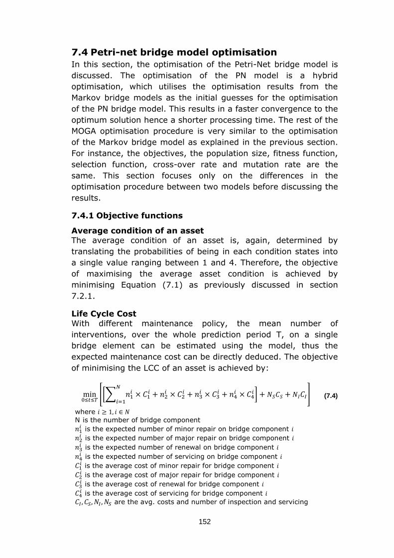
152
7.4 Petri-net bridge model optimisation
In this section, the optimisation of the Petri-Net bridge model is
discussed. The optimisation of the PN model is a hybrid
optimisation, which utilises the optimisation results from the
Markov bridge models as the initial guesses for the optimisation
of the PN bridge model. This results in a faster convergence to the
optimum solution hence a shorter processing time. The rest of the
MOGA optimisation procedure is very similar to the optimisation
of the Markov bridge model as explained in the previous section.
For instance, the objectives, the population size, fitness function,
selection function, cross-over rate and mutation rate are the
same. This section focuses only on the differences in the
optimisation procedure between two models before discussing the
results.
7.4.1 Objective functions
Average condition of an asset The average condition of an asset is, again, determined by
translating the probabilities of being in each condition states into
a single value ranging between 1 and 4. Therefore, the objective
of maximising the average asset condition is achieved by
minimising Equation (7.1) as previously discussed in section
7.2.1.
Life Cycle Cost
With different maintenance policy, the mean number of
interventions, over the whole prediction period T, on a single
bridge element can be estimated using the model, thus the
expected maintenance cost can be directly deduced. The objective
of minimising the LCC of an asset is achieved by:
[[∑
] ] (7.4)
where
N is the number of bridge component
is the expected number of minor repair on bridge component
is the expected number of major repair on bridge component
is the expected number of renewal on bridge component
is the expected number of servicing on bridge component
is the average cost of minor repair for bridge component
is the average cost of major repair for bridge component
is the average cost of renewal for bridge component
is the average cost of servicing for bridge component
are the avg. costs and number of inspection and servicing
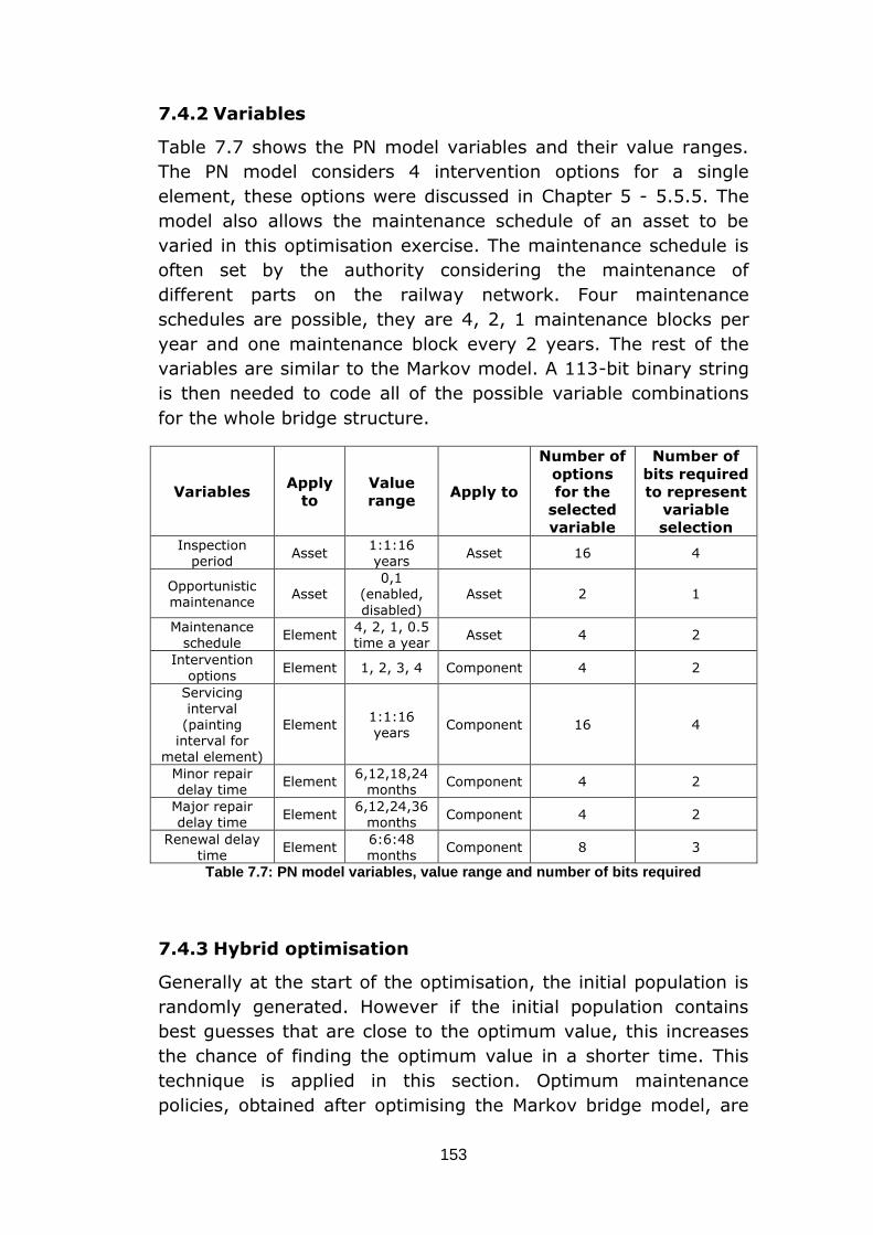
153
7.4.2 Variables
Table 7.7 shows the PN model variables and their value ranges.
The PN model considers 4 intervention options for a single
element, these options were discussed in Chapter 5 - 5.5.5. The
model also allows the maintenance schedule of an asset to be
varied in this optimisation exercise. The maintenance schedule is
often set by the authority considering the maintenance of
different parts on the railway network. Four maintenance
schedules are possible, they are 4, 2, 1 maintenance blocks per
year and one maintenance block every 2 years. The rest of the
variables are similar to the Markov model. A 113-bit binary string
is then needed to code all of the possible variable combinations
for the whole bridge structure.
Variables Apply
to
Value
range Apply to
Number of
options
for the
selected
variable
Number of
bits required
to represent
variable
selection Inspection
period Asset
1:1:16 years
Asset 16 4
Opportunistic maintenance
Asset 0,1
(enabled,
disabled)
Asset 2 1
Maintenance schedule
Element 4, 2, 1, 0.5 time a year
Asset 4 2
Intervention options
Element 1, 2, 3, 4 Component 4 2
Servicing interval
(painting interval for
metal element)
Element 1:1:16 years
Component 16 4
Minor repair delay time
Element 6,12,18,24
months Component 4 2
Major repair delay time
Element 6,12,24,36
months Component 4 2
Renewal delay time
Element 6:6:48 months
Component 8 3
Table 7.7: PN model variables, value range and number of bits required
7.4.3 Hybrid optimisation
Generally at the start of the optimisation, the initial population is
randomly generated. However if the initial population contains
best guesses that are close to the optimum value, this increases
the chance of finding the optimum value in a shorter time. This
technique is applied in this section. Optimum maintenance
policies, obtained after optimising the Markov bridge model, are
154
used as starting points (initial population) in the optimisation of
the PN model. This technique will be referred as the hybrid
optimisation since the optimisation of the PN bridge model
actually involves the optimisation of the Markov bridge model as
well. The hybrid optimisation is possible in this case because:
firstly, both the Markov and the PN model analyse the same
asset,
secondly, the two models share similar optimisation
variables (e.g. intervention options, inspection period,
servicing interval, repair delay time). Since the PN model is
effectively a more detailed bridge model compared with the
Markov model, it allows a wider range of maintenance
policies to be applied,
thirdly, the time it takes to run and optimise the Markov
model is significantly faster than the PN model.
Initial population
Where possible, each optimisation variable in the PN model is
directly mapped from the variable in the Markov model. For
example, for a single bridge element, there are three intervention
options in the Markov bridge model, they are equivalent to the
1st, 2nd, and 4th intervention option in the PN model. Similarly, the
mapping can be done for other optimisation variables, except for
the maintenance schedule variable as they were not included in
the Markov model. Hence, random values within the given value
range (Table 7.7) are generated for these variables.
Figure 7.8 illustrates a population which contains the best-
guessed individuals and the randomly generated individuals. The
green squares represent an initial population of randomly
generated individuals. The red squares represent a population of
20 best-guessed individuals that are based on the maintenance
policies obtained after optimising the Markov model. It can be
clearly seen that, the guessed-individuals form a group that is
closer to the origin than the randomly generated individuals. This
means that, the hybrid optimisation process starts with a
population that contains fitter individuals.
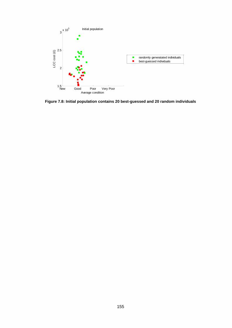
155
Figure 7.8: Initial population contains 20 best-guessed and 20 random individuals
New Good Poor Very Poor1.5
2
2.5
3x 10
5
Average condition
LC
C c
ost
(£)
Initial population
randomly generatated individuals
best-guessed individuals
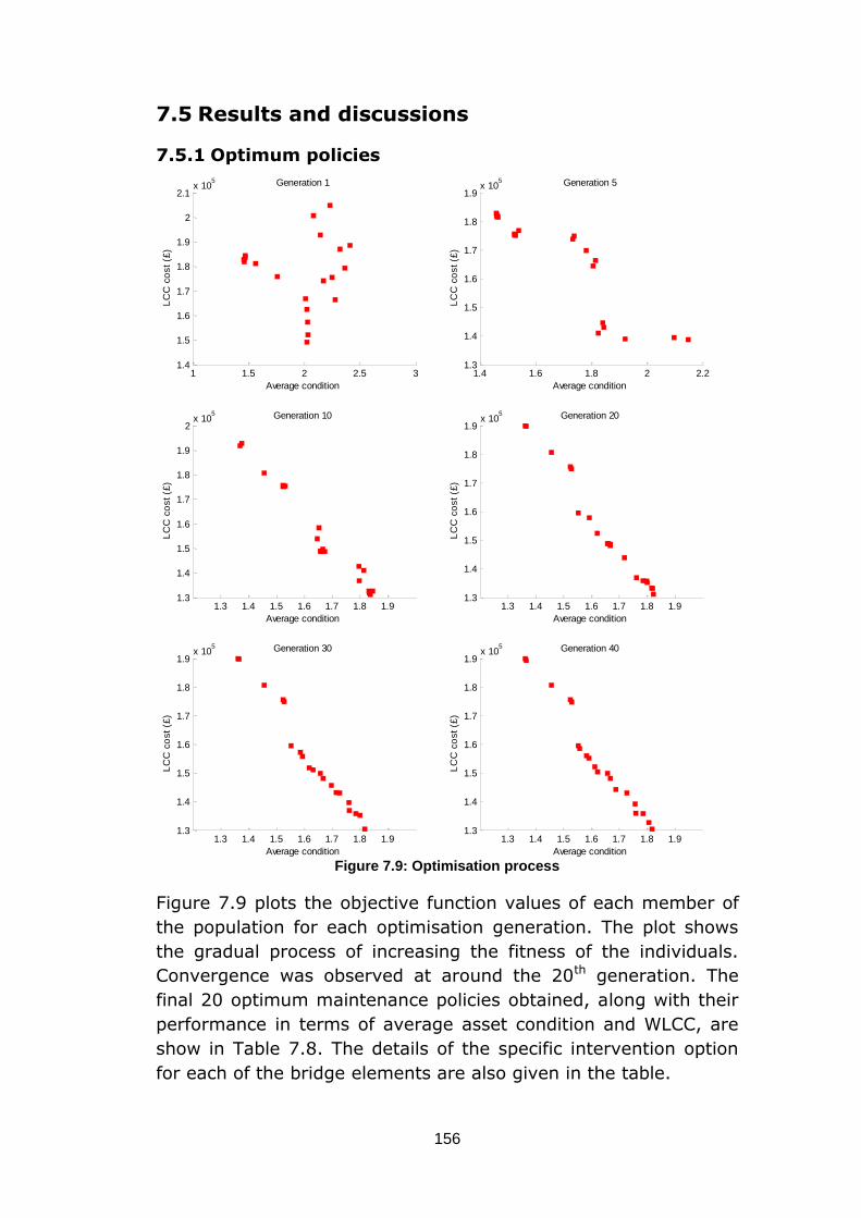
156
7.5 Results and discussions
7.5.1 Optimum policies
Figure 7.9: Optimisation process
Figure 7.9 plots the objective function values of each member of
the population for each optimisation generation. The plot shows
the gradual process of increasing the fitness of the individuals.
Convergence was observed at around the 20th generation. The
final 20 optimum maintenance policies obtained, along with their
performance in terms of average asset condition and WLCC, are
show in Table 7.8. The details of the specific intervention option
for each of the bridge elements are also given in the table.
1 1.5 2 2.5 31.4
1.5
1.6
1.7
1.8
1.9
2
2.1x 10
5
Average condition
LC
C c
ost
(£)
Generation 1
1.4 1.6 1.8 2 2.21.3
1.4
1.5
1.6
1.7
1.8
1.9x 10
5
Average condition
LC
C c
ost
(£)
Generation 5
1.3 1.4 1.5 1.6 1.7 1.8 1.91.3
1.4
1.5
1.6
1.7
1.8
1.9
2x 10
5
Average condition
LC
C c
ost
(£)
Generation 10
1.3 1.4 1.5 1.6 1.7 1.8 1.91.3
1.4
1.5
1.6
1.7
1.8
1.9x 10
5
Average condition
LC
C c
ost
(£)
Generation 20
1.3 1.4 1.5 1.6 1.7 1.8 1.91.3
1.4
1.5
1.6
1.7
1.8
1.9x 10
5
Average condition
LC
C c
ost
(£)
Generation 30
1.3 1.4 1.5 1.6 1.7 1.8 1.91.3
1.4
1.5
1.6
1.7
1.8
1.9x 10
5
Average condition
LC
C c
ost
(£)
Generation 40

157
The first 6 maintenance policies have chosen the option to
intervene as soon as any component degrades into the state
where repair is possible. This reflects the intention to maximise
the asset average condition by carrying out repair as soon as
possible. These policies are expected to keep the asset condition
very close to the ‘as new’ condition, although the associated LCC
would be higher than other policies.
Policy ID Intervention option Component Average
condition LCC over 60 years
1 Repair as soon as possible all components 1.36 139493
2 Repair as soon as possible all components 1.43 136278
3 Repair as soon as possible all components 1.46 131968
4 Repair as soon as possible all components 1.46 130597
5 Repair as soon as possible all components 1.52 128700
6 Repair as soon as possible all components 1.53 125478
7 Only carry out minor repair and replacement for:* MGI ABT1 1.55 110505
8 Only carry out minor repair and replacement for:* MGI ABT1 1.56 109891
9 Only carry out replacement for: * MGI ABT1 1.58 108720
10 Only carry out replacement for: * MGI ABT1 1.59 108640
11 Only carry out replacement for: * MGI ABT1 1.59 105941
12 Only carry out replacement for: * MGI ABT1 ABT2 1.61 101803
13 Only carry out replacement for: * MGI ABT1 ABT2 1.62 101428
14 Only carry out minor repair and replacement for:* MGI ABT1 ABT2 1.64 101087
15 Only carry out replacement for: * MGI ABT1 1.66 99231
16 Only carry out replacement for: * MGI ABT1 1.67 97473
17 Only carry out replacement for: * MGI ABT1 ABT2 1.68 94092
18 Only carry out replacement for: * MGI ABT1 ABT2 1.69 92791
19 Only carry out replacement for: * MGI ABT1 ABT2 1.73 88777
20 Only carry out replacement for: * MGI ABT1 ABT2 1.74 88229
Table 7.8: 20 optimum maintenance policies and their performances. Also shown is the intervention option on each component. (*) indicates the specific intervention options for the listed elements, for other elements, they are repaired as soon as
possible.
For other policies, whilst the intervention option is still set to
intervene as soon as possible for the unspecified bridge elements,
different intervention options were selected for the bridge internal
main girder (MGI) and the abutments (ABT1 and ABT2). Policies
7, 8 and 14 carry out only minor repair and replacement for the
MGI. Recalling that the initial condition of the MGI is poor, this
intervention option effectively allows the girder to deteriorate to a
very poor state for a complete replacement. After a replacement,
when the girder condition is restored to an ‘as new’ condition, the
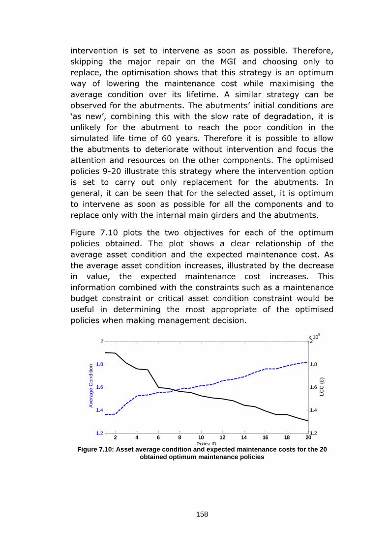
158
intervention is set to intervene as soon as possible. Therefore,
skipping the major repair on the MGI and choosing only to
replace, the optimisation shows that this strategy is an optimum
way of lowering the maintenance cost while maximising the
average condition over its lifetime. A similar strategy can be
observed for the abutments. The abutments’ initial conditions are
‘as new’, combining this with the slow rate of degradation, it is
unlikely for the abutment to reach the poor condition in the
simulated life time of 60 years. Therefore it is possible to allow
the abutments to deteriorate without intervention and focus the
attention and resources on the other components. The optimised
policies 9-20 illustrate this strategy where the intervention option
is set to carry out only replacement for the abutments. In
general, it can be seen that for the selected asset, it is optimum
to intervene as soon as possible for all the components and to
replace only with the internal main girders and the abutments.
Figure 7.10 plots the two objectives for each of the optimum
policies obtained. The plot shows a clear relationship of the
average asset condition and the expected maintenance cost. As
the average asset condition increases, illustrated by the decrease
in value, the expected maintenance cost increases. This
information combined with the constraints such as a maintenance
budget constraint or critical asset condition constraint would be
useful in determining the most appropriate of the optimised
policies when making management decision.
Figure 7.10: Asset average condition and expected maintenance costs for the 20
obtained optimum maintenance policies
2 4 6 8 10 12 14 16 18 201.2
1.4
1.6
1.8
2
Ave
rag
e C
on
ditio
n
Policy ID
2 4 6 8 10 12 14 16 18 201.2
1.4
1.6
1.8
2x 10
5
LC
C (
£)
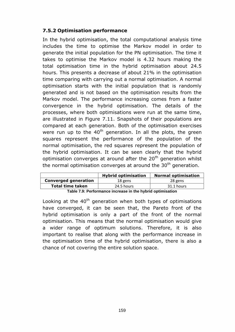
159
7.5.2 Optimisation performance
In the hybrid optimisation, the total computational analysis time
includes the time to optimise the Markov model in order to
generate the initial population for the PN optimisation. The time it
takes to optimise the Markov model is 4.32 hours making the
total optimisation time in the hybrid optimisation about 24.5
hours. This presents a decrease of about 21% in the optimisation
time comparing with carrying out a normal optimisation. A normal
optimisation starts with the initial population that is randomly
generated and is not based on the optimisation results from the
Markov model. The performance increasing comes from a faster
convergence in the hybrid optimisation. The details of the
processes, where both optimisations were run at the same time,
are illustrated in Figure 7.11. Snapshots of their populations are
compared at each generation. Both of the optimisation exercises
were run up to the 40th generation. In all the plots, the green
squares represent the performance of the population of the
normal optimisation, the red squares represent the population of
the hybrid optimisation. It can be seen clearly that the hybrid
optimisation converges at around after the 20th generation whilst
the normal optimisation converges at around the 30th generation.
Hybrid optimisation Normal optimisation
Converged generation 18 gens 28 gens Total time taken 24.5 hours 31.1 hours
Table 7.9: Performance increase in the hybrid optimisation
Looking at the 40th generation when both types of optimisations
have converged, it can be seen that, the Pareto front of the
hybrid optimisation is only a part of the front of the normal
optimisation. This means that the normal optimisation would give
a wider range of optimum solutions. Therefore, it is also
important to realise that along with the performance increase in
the optimisation time of the hybrid optimisation, there is also a
chance of not covering the entire solution space.
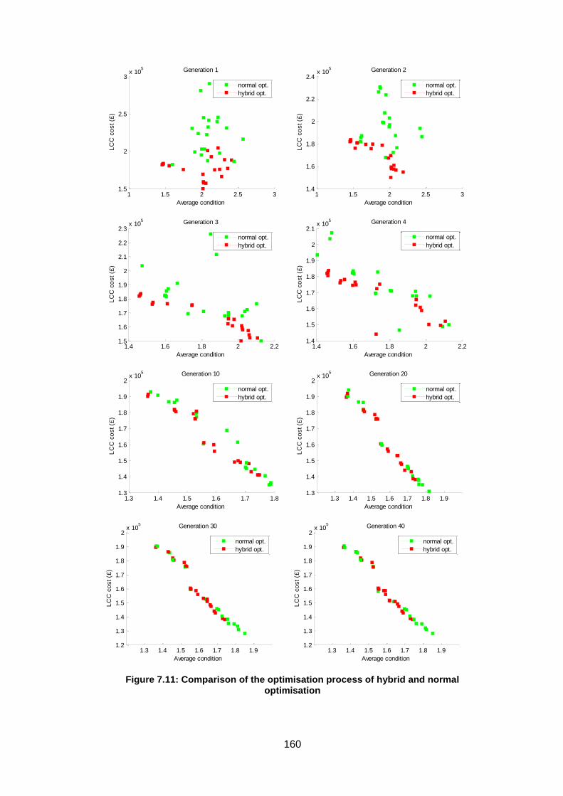
160
Figure 7.11: Comparison of the optimisation process of hybrid and normal optimisation
1 1.5 2 2.5 31.5
2
2.5
3x 10
5
Average condition
LC
C c
ost
(£)
Generation 1
normal opt.
hybrid opt.
1 1.5 2 2.5 31.4
1.6
1.8
2
2.2
2.4x 10
5
Average condition
LC
C c
ost
(£)
Generation 2
normal opt.
hybrid opt.
1.4 1.6 1.8 2 2.21.5
1.6
1.7
1.8
1.9
2
2.1
2.2
2.3x 10
5
Average condition
LC
C c
ost
(£)
Generation 3
normal opt.
hybrid opt.
1.4 1.6 1.8 2 2.21.4
1.5
1.6
1.7
1.8
1.9
2
2.1x 10
5
Average condition
LC
C c
ost
(£)
Generation 4
normal opt.
hybrid opt.
1.3 1.4 1.5 1.6 1.7 1.81.3
1.4
1.5
1.6
1.7
1.8
1.9
2x 10
5
Average condition
LC
C c
ost
(£)
Generation 10
normal opt.
hybrid opt.
1.3 1.4 1.5 1.6 1.7 1.8 1.91.3
1.4
1.5
1.6
1.7
1.8
1.9
2x 10
5
Average condition
LC
C c
ost
(£)
Generation 20
normal opt.
hybrid opt.
1.3 1.4 1.5 1.6 1.7 1.8 1.91.2
1.3
1.4
1.5
1.6
1.7
1.8
1.9
2x 10
5
Average condition
LC
C c
ost
(£)
Generation 30
normal opt.
hybrid opt.
1.3 1.4 1.5 1.6 1.7 1.8 1.91.2
1.3
1.4
1.5
1.6
1.7
1.8
1.9
2x 10
5
Average condition
LC
C c
ost
(£)
Generation 40
normal opt.
hybrid opt.
161
7.6 Summary
An optimisation framework based on the Genetic Algorithm
technique was used in this chapter as a decision making approach
to select the best maintenance strategies. The optimisation was
applied on both of the Markov and the Petri-Net bridge models.
The optimisation is a multi-objective optimisation that looks for
the maintenance policies that will produce the lowest expected
maintenance cost whilst maximising the average condition of the
asset.
This chapter starts with the optimisation of the Markov bridge
model. The optimisation procedure including the evaluation of the
objectives, variable coding, fitness, selection functions, etc., are
discussed in detail. The results present 20 optimum maintenance
policies. A policy was chosen from the set of optimised policies
that shows an improved performance when compared with the
current industry maintenance policy.
Following this, the optimisation of the Petri-Net bridge model is
discussed. The optimisation for the PN model is a hybrid approach
which utilises the final results from optimising the Markov bridge
model. These results provide an initial population for the PN
model optimisation. With this better initial population, the
optimisation process was able to converge to the optimum
solutions quicker, resulting in a performance increase of 21%
faster in the optimisation time.
Overall, this chapter provides an optimisation framework for the
bridge models. The optimal maintenance policies obtained
represent a wide variety of maintenance strategies for the chosen
asset. These policies would assist the decision making process by
not only providing a number of solutions, but also justifying the
decision to carry out repairs or let a component continue to
deteriorate to the point where it is replaced. Combining this with
the expert judgement and engineering knowledge, the optimum
maintenance policy can be identified.
162
Chapter 8 - Conclusions
8.1 Summary and conclusions
Bridges are an important part of the railway network. As bridges
age, the management authorities are faced with the increasing
pressure to keep the bridge in an acceptable condition accounting
for budgetary constraints and the need to avoid service
disruptions. The main objective of the research presented in this
thesis is to develop a complete bridge asset state model. The key
element of the model is to establish the deterioration
characteristics of each of the bridge components. This has been
achieved by the analyses of historical maintenance data. The
model can give an accurate prediction of the asset future
condition and can be used to demonstrate the effects of different
maintenance strategies. An optimisation framework has been
developed as a decision making approach to select the best
maintenance policies. The optimum maintenance policy will be
that which produces the lowest expected maintenance costs
whilst maximising the average condition of the asset.
Following an extensive literature review on the existing bridge
condition models, the needs for a more robust and detailed model
were identified. The majority of bridge models have adopted the
Markov chain method in predicting the deterioration process and
future bridge element conditions. These models are simple and
lack application and verification on real data. The Markov
modelling approach also has several associated limitations such
as: constant transition rates and the size of the model becomes
163
unmanageable when the problem is complex. In addition when
forming a bridge model in terms of its component conditions the
complete asset model cannot be constructed by combining the
component models, a completely new model form has to be
generated. Other modelling techniques such as semi-Markov and
reliability-based approaches have been developed. However,
whilst having the potential to overcome the constant failure rate
restriction, they have not provided a complete solution to the
other issues in bridge asset modelling. Furthermore, all of the
reviewed models are based on statistical analysis of condition
ratings. It was identified that this data source is inadequate for a
bridge degradation study.
The research proposed a study to understand the bridge
deterioration based on analysing the recorded historical work
done on bridge elements as an alternative to the use of condition
ratings. By constructing a life history of each component and
grouping similar components according to their structure types
and materials, a statistical analysis was performed to model the
characteristic behaviour of a given bridge element type. In this
analysis, the Weibull distribution is fitted to the times for a
component to reach different condition states (good, poor, very
poor states). The study was carried out to model the degradation
process for major bridge elements (main girders, deck, bearing,
and abutment). The analysis suggested that the degradation rates
of bridge elements are not constant and increases slowly over
time. The degradation modelling forms the foundation to the
development of a complete bridge model.
There are two bridge models that have been developed in this
research. The first model is based on the Markov modelling
approach, which is a widely accepted approach in bridge
modelling. The second model is based on the Petri-Net method,
which has never been applied to bridge modelling. In the
development of the first model, a considerable level of detail has
been introduced. The model accounts for the initial condition of
bridge elements, material type, structure type, environment,
inspection intervals, servicing intervals, repair strategy,
opportunistic repair and repair scheduling times. All these model
parameters can be varied to investigate the effects of different
maintenance scenarios. The effects of a specified maintenance
strategy is reflected in terms of the probabilities of the bridge

164
elements being in different states at a given time in the future;
and the expected maintenance cost over the entire prediction
period. Application of the Markov bridge model has provided an
insight into this modelling technique, understanding both the
capabilities and the limitations and providing a bridge modelling
framework that can be used for the validation of the second
bridge model developed.
It was shown that, even though the Markov model is capable of
detailed modelling, a more flexible and robust approach is
required. Therefore, a second bridge model was developed which
is based on the Petri-Net (PN) approach. The PN approach is
increasingly being used to model dynamic systems, and in this
research, a number of modifications to the traditional PN concept
have been made to suit the problem in bridge asset management.
The PN model not only keeps the level of complexity that was
developed in the Markov model but also further increases the
level of modelling detail. One of the most important features is
the capability of incorporating the non-constant deterioration
rates of bridge elements. Furthermore, the PN model models the
degradation process of the protective coating for metal elements.
It also realises some repairs are ineffective after a number of
times carried out and the planning of repairs accounts for
different maintenance schedules according to the criticality of the
asset. A Monte Carlo simulation was used to simulate the model
and the statistics collected indicate the performance of the bridge
and its elements.
The results and performances of the two models can be compared
by applying, as near as possible, the same maintenance policy on
the same asset. It is worth noting that, with the increasing level
of details in the PN model, the results obtained from the two
models will not be exactly the same, however it is expected that
they should be very close to each other. The comparison study
confirmed that both models predict very similar future average
conditions. This validates the PN approach to the modelling of
bridge assets. The comparison also shows that the PN bridge
model predicts more informative on the asset condition profiles in
the near future. This information can be useful in the way that the
inspection and maintenance can be allocated accordingly.
Moreover, the PN model is more efficient in the execution time
when a system contains many components.

165
These models provide a means of investigating the effects of
different maintenance policies. Based on the bridge models, an
optimisation framework has been developed to find the optimum
maintenance policies such that the average asset condition is
maximised whilst the expected maintenance cost is minimised.
Optimisation studies were carried out for both models and the
results present a set of 20 optimum maintenance policies. A
policy was chosen from the set of optimised policies that shows
an improved performance when compared with the current
industry maintenance policy. It was realised that for a complex
optimisation problem, where many system evaluations will be
required, that the efficiency of the optimisation process is
important. To address this, the research developed a hybrid
optimisation framework, which utilises the optimisation results
from the Markov bridge model as initial guesses for the
optimisation of the PN bridge model. An 21% reduction in the
optimisation time was achieved using the hybrid optimisation. The
maintenance optimisation provides a wide range of optimum
policies that would assist the decision making process and
combined with the engineering judgements, the optimum policy
for a bridge asset can be selected.
The proposed bridge model delivers a tool for the bridge
management authorities and decision makers to assess the
degradation process and investigate the effects of different
maintenance policies on bridge assets. The model can be
employed to determine cost-effective bridge maintenance
strategies while maintaining a desirable bridge condition.
8.2 Research contributions
Based on the current developments, this research makes a
number of contributions:
Better understanding of bridge asset management
needs: This research has reviewed a number of studies and
the shortcomings in current modelling approaches have
been identified. The needs for a new approach, as well as
the several practical modelling requirements, were
understood through meetings and discussions with bridge
experts and the bridge management authority.
166
The use of historical maintenance data: Instead of
bridge condition rating data, the research used historical
work done data when formulating the degradation models.
The maintenance effects is captured and analysed with this
data.
The estimation of the degradation process for a single
component given a degradation process of a group of
similar components: Many bridge elements exist in
quantities greater than one on a structure. In this case the
maintenance work carried out is often only attributed to the
component type and does not specify which one. The
degradation analysis then gives the degradation
characteristic of the set of components. A method based on
simulation was developed in this research to estimate the
degradation process of each individual component using this
data.
Better understanding of the degradation processes of
several major bridge elements: the study has presented
the analysis for metal underbridge’ major elements such as:
metal girder, concrete deck, metal deck, timber deck, metal
bearing, and masonry abutment.
The consideration of many factors that affects the
deterioration and maintenance planning process:
Environment, the increasing deterioration rates of bridge
elements, the degradation process of protective coatings for
metal elements, inspection intervals, servicing intervals,
level of intervention, opportunistic repair and repair
scheduling times are the factors included in the models
proposed.
The application of the Petri-Net approach to bridge
assets modelling: The main advantage of this research is
the development of the Petri-Net bridge model. The
flexibility and capability of the approach offers a more
robust modelling for bridge asset management, its
advantages have been presented and discussed throughout
the thesis. The model allows easy expansion (i.e. more
detail modelling) and the opportunity to expand the model
to system level with integrated asset modelling.
The application of the hybrid optimisation: The
optimisation performance increases with the use of the
167
hybrid optimisation approach resulting in a shorter
optimisation times.
8.3 Future works
Despite the capabilities and benefits of the research, there are
several areas in which further work can be carried out:
The current assumption of the bridge models is that repairs
are perfect i.e. maintenance restores the component
condition to the ‘as good as new’ condition. More research is
needed in order to determine the effect of the repair on the
component condition as well as the degradation process
after each time the repair is carried out.
It is anticipated that the analysis of more complex problems
would require more computational effort. Therefore future
work should be focused on improving the efficiency of the
analysis, especially the efficiency of the computer coding to
reduce the solution time.
There are only three types of interventions considered in
this research due to the limited availability of the historical
data. With more data becomes available, more specific
works can be modelled, this means that more types of
component defects are considered. For this purpose, extra
model states can be added to accommodate the increasing
level of modelling detail.
In the research presented in this thesis, the Genetic
Algorithm (GA) was used as the optimisation method. This
has proven to be sufficient enough for the optimisation
problem presented. However, other advanced GAs and
hybrid heuristic techniques provide potential alternatives.
Research could be performed to improve the search ability
and computational efficiency of such approaches.
Future work should focus on the development of bridge
models for other asset types (e.g. overbridges) and
ultimately, the development of a complete network model
which allows the asset management of entire railway
network to be modelled as a system.
168
References
AGRAWAL, A. K. & KAWAGUCHI, A. 2009. Bridge element
deterioration rates. New York State Department of
Transportation. AGRAWAL, A. K., KAWAGUCHI, A. & CHEN, Z. 2010. Deterioration
rates of typical bridge elements in New York. Journal of Bridge Engineering, 15, 419-429.
ANDREWS, J. 2013. A modelling approach to railway track asset management. Proceedings of the Institution of Mechanical
Engineers, Part F: Journal of Rail and Rapid Transit, 227, 56-73.
ANDREWS, J. D. & MOSS, T. R. 2002. Reliability and Risk Assessment, London and Bury St Edmunds, UK, Professional
Engineering Publishing Limited. BAUSE, F. & KRITZINGER, P. S. 2002. Stochastic Petri Nets,
Springer. BU, G., SON, J., LEE, J., GUAN, H., BLUMENSTEIN, M. & LOO, Y.
2013. Typical deterministic and stochastic bridge
deterioration modelling incorporating backward prediction model. Journal of Civil Structural Health Monitoring, 1-12.
BUTT, A. A., SHAHIN, M., CARPENTER, S. & CARNAHAN, J. Application of Markov process to pavement management
systems at network level. 3rd International Conference on Managing Pavements, 1994. 159-172.
CESARE, M. A., SANTAMARINA, C., TURKSTRA, C. & VANMARCKE, E. H. 1991. Modelling Bridge Deterioration With Markov
Chains. Journal of Transportation Engineering, 118, 2237. CESARE, M. A., SANTAMARINA, C., TURKSTRA, C. & VANMARCKE,
E. H. 1992. Modeling bridge deterioration with Markov chains. Journal of Transportation Engineering, 118, 820-
833. CHIOLA, G., MARSAN, M. A., BALBO, G. & CONTE, G. 1993.
Generalized stochastic Petri nets: A definition at the net
level and its implications. Software Engineering, IEEE Transactions on, 19, 89-107.
CIARDO, G., MUPPALA, J. & TRIVEDI, T. SPNP: stochastic Petri net package. Petri Nets and Performance Models, 1989.
PNPM89., Proceedings of the Third International Workshop on, 11-13 Dec 1989 1989. 142-151.
DESTEFANO, P. D. & GRIVAS, D. A. 1998. Method for estimating transition probability in bridge deterioration models. Journal
of Infrastructure Systems, 4, 56-62.
169
FONSECA, C. M. & FLEMING, P. J. Genetic Algorithms for Multiobjective Optimization: FormulationDiscussion and
Generalization. ICGA, 1993. 416-423. FRANGOPOL, D. M., KONG, S. J. & GHARAIBEH, S. E. 2001.
Reliability-based life-cycle management of Highway bridges. Journal of Computing in Civil Engineering, 15, 27-34.
FRANGOPOL, D. M., YANG, S.-I. & NEVES, L. C. 2006. Optimum
maintenance strategy for deteriorating bridge structures based on lifetime functions. Engineering Structures, Vol. 28,
pg. 196-206. GIRAULT, C. & VALK, R. 2002. Petri nets for systems engineering:
a guide to modeling, verification, and applications, Springer. HALCROW 2011. Bridges Tier 2 Whole Life Cycle Cost Model -
Phase 1. In: NETWORKRAIL (ed.) Bridges Tier 2 Whole Life Cycle Cost Model.
HAUPT, R. L. & HAUPT, S. E. 2004. Practical genetic algorithms, Wiley-Interscience.
HEARN, G., THOMPSON, P. D. & HYMAN, W. 2010. Framework for a National Database System for Maintenance Actions on
Highway Bridges. WASHINGTON, D.C. HOLLAND, J. H. 1975. Adaptation in natural and artificial
systems: an introductory analysis with applications to
biology, control, and artificial intelligence, University of Michigan Press.
HOLLIDAY, M. A. & VERNON, M. K. 1987. A generalized timed Petri net model for performance analysis. Software
Engineering, IEEE Transactions on, 1297-1310. IBE, O. C. 2009. Markov Processes for Stochastic Modeling,
Academic Press. JENSEN, K. 1996. Coloured Petri Nets: Basic Concepts, Analysis
Methods and Practical Use, Springer. JENSEN, K. & KRISTENSEN, L. M. 2009. Coloured petri nets,
Springer. JIANG, Y. & SINHA, K. C. 1989. Bridge service life prediction
model using the Markov chain. Transportation Research Record, 24-30.
KLEINER, Y. 2001. Scheduling inspection and renewal of large
infrastructure assets. Journal of Infrastructure Systems, 7, 136-143.
MALHOTRA, M. & TRIVEDI, K. S. 1995. Dependability modeling using Petri-nets. Reliability, IEEE Transactions on, 44, 428-
440. MARSAN, M. A., BALBO, G., CONTE, G., DONATELLI, S. &
FRANCESCHINIS, G. 1998. Modelling with generalized stochastic petri nets. ACM SIGMETRICS Performance
Evaluation Review, 26, 2. MISHALANI, R. G. & MADANAT, S. M. 2002. Computation of
infrastructure transition probabilities using stochastic
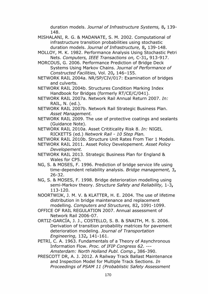
170
duration models. Journal of Infrastructure Systems, 8, 139-148.
MISHALANI, R. G. & MADANATE, S. M. 2002. Computational of infrastructure transition probabilities using stochastic
duration models. Journal of Infrastructure, 8, 139-148. MOLLOY, M. K. 1982. Performance Analysis Using Stochastic Petri
Nets. Computers, IEEE Transactions on, C-31, 913-917.
MORCOUS, G. 2006. Performance Prediction of Bridge Deck Systems Using Markov Chains. Journal of Performance of
Constructed Facilities, Vol. 20, 146–155. NETWORK RAIL 2004a. NR/SP/CIV/017: Examination of bridges
and culverts. NETWORK RAIL 2004b. Structures Condition Marking Index
Handbook for Bridges (formerly RT/CE/C/041). NETWORK RAIL 2007a. Network Rail Annual Return 2007. In:
RAIL, N. (ed.). NETWORK RAIL 2007b. Network Rail Strategic Business Plan.
Asset Management. NETWORK RAIL 2009. The use of protective coatings and sealants
(Guidance Note). NETWORK RAIL 2010a. Asset Crititicality Risk 8. In: NIGEL
RICKETTS (ed.) Network Rail - 10 Step Plan.
NETWORK RAIL 2010b. Structure Unit Rates From Tier 1 Models. NETWORK RAIL 2011. Asset Policy Developement. Asset Policy
Developement. NETWORK RAIL 2013. Strategic Business Plan for England &
Wales for CP5. NG, S. & MOSES, F. 1996. Prediction of bridge service life using
time-dependent reliability analysis. Bridge management, 3, 26-32.
NG, S. & MOSES, F. 1998. Bridge deterioration modelling using semi-Markov theory. Structure Safety and Reliability, 1-3,
113-120. NOORTWIJK, J. M. V. & KLATTER, H. E. 2004. The use of lifetime
distribution in bridge maintenance and replacement modelling. Computers and Structures, 82, 1091-1099.
OFFICE OF RAIL REGULATION 2007. Annual assessment of
Network Rail 2006-07. ORTIZ-GARCÍA, J. J., COSTELLO, S. B. & SNAITH, M. S. 2006.
Derivation of transition probability matrices for pavement deterioration modeling. Journal of Transportation
Engineering, 132, 141-161. PETRI, C. A. 1963. Fundamentals of a Theory of Asynchronous
Information Flow. Proc. of IFIP Congress 62. --- Amsterdam: North Holland Publ. Comp., 386-390.
PRESCOTT DR, A. J. 2012. A Railway Track Ballast Maintenance and Inspection Model for Multiple Track Sections. In
Proceedings of PSAM 11 (Probablistic Safety Assessment
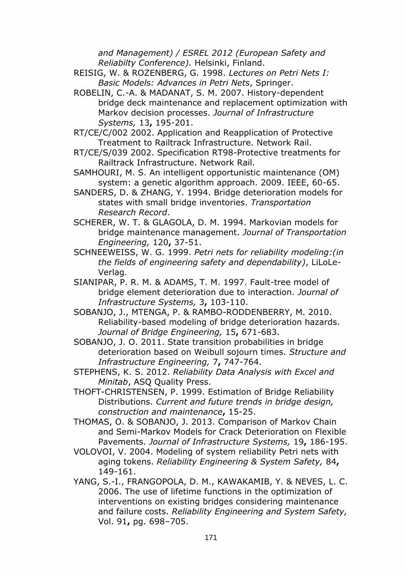
171
and Management) / ESREL 2012 (European Safety and Reliabilty Conference). Helsinki, Finland.
REISIG, W. & ROZENBERG, G. 1998. Lectures on Petri Nets I: Basic Models: Advances in Petri Nets, Springer.
ROBELIN, C.-A. & MADANAT, S. M. 2007. History-dependent bridge deck maintenance and replacement optimization with
Markov decision processes. Journal of Infrastructure
Systems, 13, 195-201. RT/CE/C/002 2002. Application and Reapplication of Protective
Treatment to Railtrack Infrastructure. Network Rail. RT/CE/S/039 2002. Specification RT98-Protective treatments for
Railtrack Infrastructure. Network Rail. SAMHOURI, M. S. An intelligent opportunistic maintenance (OM)
system: a genetic algorithm approach. 2009. IEEE, 60-65. SANDERS, D. & ZHANG, Y. 1994. Bridge deterioration models for
states with small bridge inventories. Transportation Research Record.
SCHERER, W. T. & GLAGOLA, D. M. 1994. Markovian models for bridge maintenance management. Journal of Transportation
Engineering, 120, 37-51. SCHNEEWEISS, W. G. 1999. Petri nets for reliability modeling:(in
the fields of engineering safety and dependability), LiLoLe-
Verlag. SIANIPAR, P. R. M. & ADAMS, T. M. 1997. Fault-tree model of
bridge element deterioration due to interaction. Journal of Infrastructure Systems, 3, 103-110.
SOBANJO, J., MTENGA, P. & RAMBO-RODDENBERRY, M. 2010. Reliability-based modeling of bridge deterioration hazards.
Journal of Bridge Engineering, 15, 671-683. SOBANJO, J. O. 2011. State transition probabilities in bridge
deterioration based on Weibull sojourn times. Structure and Infrastructure Engineering, 7, 747-764.
STEPHENS, K. S. 2012. Reliability Data Analysis with Excel and Minitab, ASQ Quality Press.
THOFT-CHRISTENSEN, P. 1999. Estimation of Bridge Reliability Distributions. Current and future trends in bridge design,
construction and maintenance, 15-25.
THOMAS, O. & SOBANJO, J. 2013. Comparison of Markov Chain and Semi-Markov Models for Crack Deterioration on Flexible
Pavements. Journal of Infrastructure Systems, 19, 186-195. VOLOVOI, V. 2004. Modeling of system reliability Petri nets with
aging tokens. Reliability Engineering & System Safety, 84, 149-161.
YANG, S.-I., FRANGOPOLA, D. M., KAWAKAMIB, Y. & NEVES, L. C. 2006. The use of lifetime functions in the optimization of
interventions on existing bridges considering maintenance and failure costs. Reliability Engineering and System Safety,
Vol. 91, pg. 698–705.

172
YANG, Y. N., PAM, H. J. & KUMARASWAMY, M. M. 2009. Framework Development of Performance Prediction Models
for Concrete Bridges. Journal of Transportation Engineering, 135, 545-554.

173
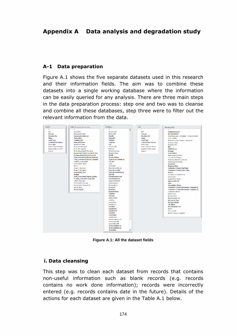
174
Appendix A Data analysis and degradation study
A-1 Data preparation
Figure A.1 shows the five separate datasets used in this research
and their information fields. The aim was to combine these
datasets into a single working database where the information
can be easily queried for any analysis. There are three main steps
in the data preparation process: step one and two was to cleanse
and combine all these databases, step three were to filter out the
relevant information from the data.
Figure A.1: All the dataset fields
i. Data cleansing
This step was to clean each dataset from records that contains
non-useful information such as blank records (e.g. records
contains no work done information); records were incorrectly
entered (e.g. records contains date in the future). Details of the
actions for each dataset are given in the Table A.1 below.
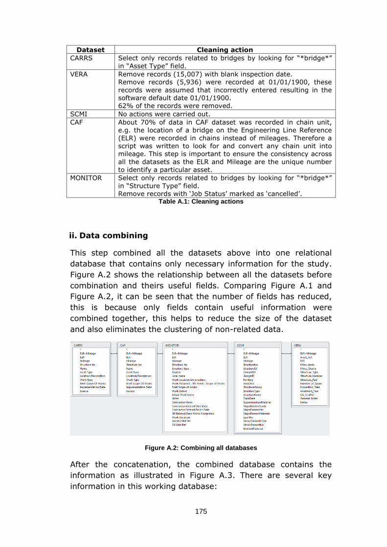
175
Dataset Cleaning action
CARRS Select only records related to bridges by looking for “*bridge*”
in “Asset Type” field.
VERA Remove records (15,007) with blank inspection date.
Remove records (5,936) were recorded at 01/01/1900, these
records were assumed that incorrectly entered resulting in the
software default date 01/01/1900.
62% of the records were removed.
SCMI No actions were carried out.
CAF About 70% of data in CAF dataset was recorded in chain unit,
e.g. the location of a bridge on the Engineering Line Reference
(ELR) were recorded in chains instead of mileages. Therefore a
script was written to look for and convert any chain unit into
mileage. This step is important to ensure the consistency across
all the datasets as the ELR and Mileage are the unique number
to identify a particular asset.
MONITOR Select only records related to bridges by looking for “*bridge*”
in “Structure Type” field.
Remove records with ‘Job Status’ marked as ‘cancelled’. Table A.1: Cleaning actions
ii. Data combining
This step combined all the datasets above into one relational
database that contains only necessary information for the study.
Figure A.2 shows the relationship between all the datasets before
combination and theirs useful fields. Comparing Figure A.1 and
Figure A.2, it can be seen that the number of fields has reduced,
this is because only fields contain useful information were
combined together, this helps to reduce the size of the dataset
and also eliminates the clustering of non-related data.
Figure A.2: Combining all databases
After the concatenation, the combined database contains the
information as illustrated in Figure A.3. There are several key
information in this working database:
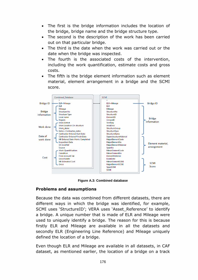
176
The first is the bridge information includes the location of
the bridge, bridge name and the bridge structure type.
The second is the description of the work has been carried
out on that particular bridge.
The third is the date when the work was carried out or the
date when the bridge was inspected.
The fourth is the associated costs of the intervention,
including the work quantification, estimate costs and gross
costs.
The fifth is the bridge element information such as element
material, element arrangement in a bridge and the SCMI
score.
Figure A.3: Combined database
Problems and assumptions
Because the data was combined from different datasets, there are
different ways in which the bridge was identified, for example,
SCMI uses ‘StructureID’; VERA uses ‘Asset_Reference’ to identify
a bridge. A unique number that is made of ELR and Mileage were
used to uniquely identify a bridge. The reason for this is because
firstly ELR and Mileage are available in all the datasets and
secondly ELR (Engineering Line Reference) and Mileage uniquely
defined the location of a bridge.
Even though ELR and Mileage are available in all datasets, in CAF
dataset, as mentioned earlier, the location of a bridge on a track
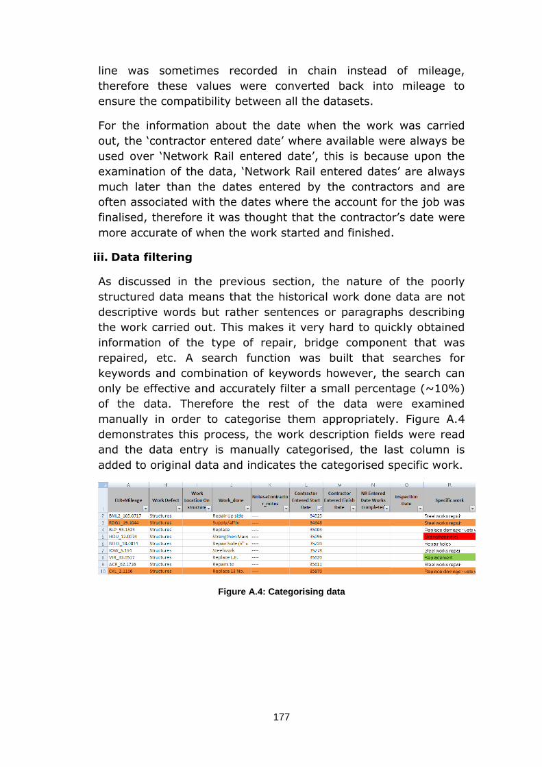
177
line was sometimes recorded in chain instead of mileage,
therefore these values were converted back into mileage to
ensure the compatibility between all the datasets.
For the information about the date when the work was carried
out, the ‘contractor entered date’ where available were always be
used over ‘Network Rail entered date’, this is because upon the
examination of the data, ‘Network Rail entered dates’ are always
much later than the dates entered by the contractors and are
often associated with the dates where the account for the job was
finalised, therefore it was thought that the contractor’s date were
more accurate of when the work started and finished.
iii. Data filtering
As discussed in the previous section, the nature of the poorly
structured data means that the historical work done data are not
descriptive words but rather sentences or paragraphs describing
the work carried out. This makes it very hard to quickly obtained
information of the type of repair, bridge component that was
repaired, etc. A search function was built that searches for
keywords and combination of keywords however, the search can
only be effective and accurately filter a small percentage (~10%)
of the data. Therefore the rest of the data were examined
manually in order to categorise them appropriately. Figure A.4
demonstrates this process, the work description fields were read
and the data entry is manually categorised, the last column is
added to original data and indicates the categorised specific work.
Figure A.4: Categorising data
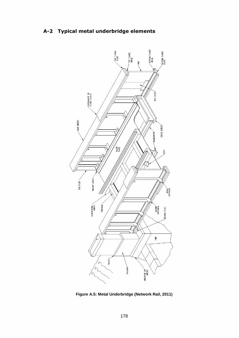
178
A-2 Typical metal underbridge elements
Figure A.5: Metal Underbridge (Network Rail, 2011)

179
A-3 Element condition states
The condition of an element is decided based on the significant of
a defect discovered. Network Rail’s standards uses the term
Severity and Extent (SevEx) to quantify a component defect. The
definitions of the SevEx (Network Rail, 2004b) of defects on
metallic element are given in Figure A.6. The SevEx shows the
seriousness of defects and also give the idea of the degradation
process on a metal bridge element. A given combination of
severity and extent (e.g. A2) indicates a particular type of defect,
however many defects can be grouped together indicating the
same level of degradation i.e. a certain condition state. By
studying the combination of them different levels of degradation
can be seen.
Table A.2 shows all the combinations of SevEx and the four
condition states for a metal element.
Element with no visible defects (B2) to localise corrosion/ loss of
section up to 5mm deep (C2 or B3), it is only minor defects and
would be considered to be in an ‘as new’ state.
Element with minor corrosion defects is when the corrosion/loss
of section is less than 1mm deep but occupies up to 10% of the
surface of the element; up to the corrosion defects that more
than 10mm deep and occupies more than 50% surface area of
the element. The element is considered to be in a good state.
Major corrosion is when localised corrosion / loss of section have
taken out the full thickness of the element section up to the case
when the loss of the full thickness of the section is not localised
and has spread up to 5% surface area of the element. This is poor
state.
The very poor state is when the element experiences major
distortion i.e. when the element is torn, fractured, buckled or
permanently distorted, this type of defects often seriously affects
the structural capability of the elements and would generally
require immediate attention and a complete replacement of the
failed component.
For components of different materials (concrete, timber,
masonry), the definition of the SevEx and condition states are
also given below (Figure A.7 to A.9 and Table A.3 to Table A.5).
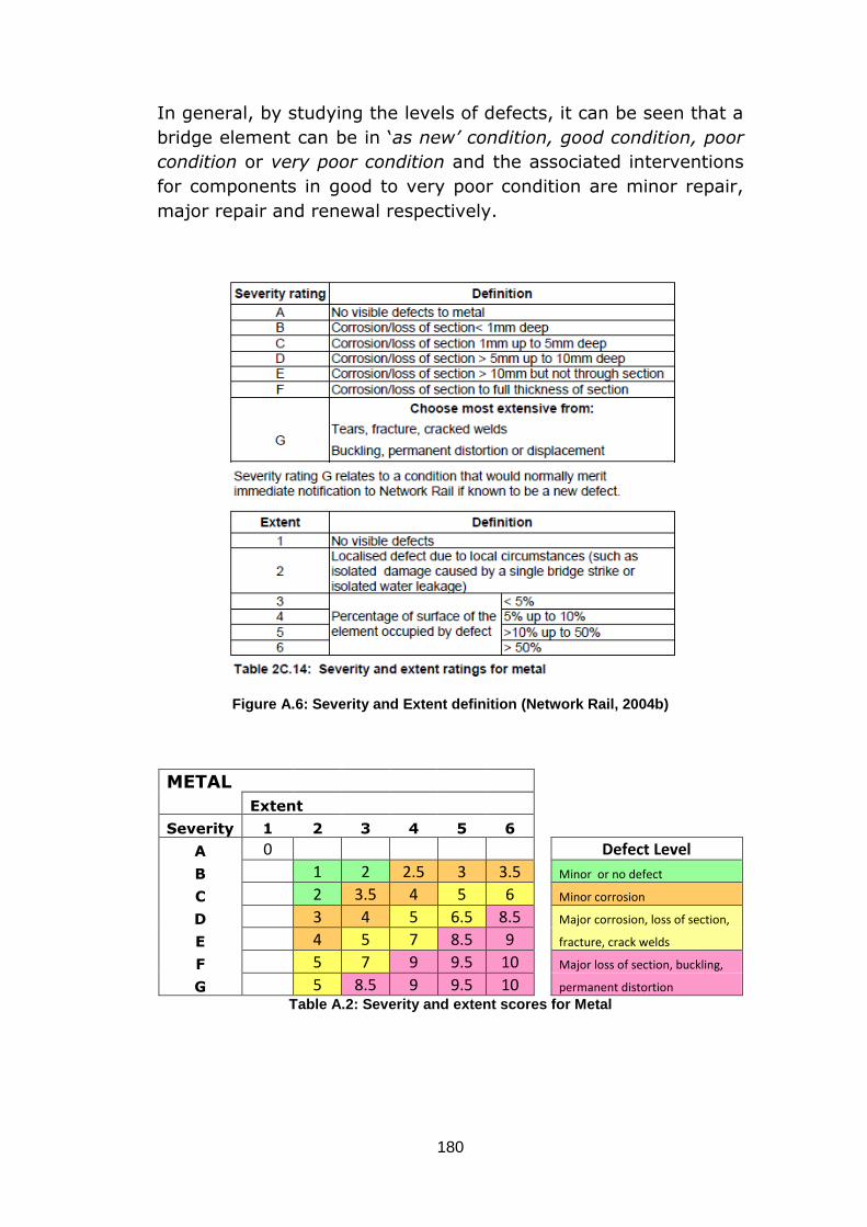
180
In general, by studying the levels of defects, it can be seen that a
bridge element can be in ‘as new’ condition, good condition, poor
condition or very poor condition and the associated interventions
for components in good to very poor condition are minor repair,
major repair and renewal respectively.
Figure A.6: Severity and Extent definition (Network Rail, 2004b)
METAL Extent Severity 1 2 3 4 5 6
A 0
Defect Level
B 1 2 2.5 3 3.5
Minor or no defect
C 2 3.5 4 5 6
Minor corrosion
D 3 4 5 6.5 8.5
Major corrosion, loss of section,
E 4 5 7 8.5 9
fracture, crack welds
F 5 7 9 9.5 10
Major loss of section, buckling,
G 5 8.5 9 9.5 10
permanent distortion Table A.2: Severity and extent scores for Metal

181
Figure A.7: Severity and Extent definition for Concrete
CONCRETE Extent Severity 1 2 3 4 5 6
A 0
Defect Level
B 1 1.5 2 2.5 3
Minor surface damage
C 1.5 2 3 4.5 5.5
Spalling, small cracks, exposed of
D 2 3 3.5 4.5 6
secondary reinforcement
E 3 4 4.5 5 7
Exposed of primary reinforcement
F 5 5 6 7.5 9
Permanent structural damage
G 8 8 9 10 10 Table A.3: Severity and Extent scores for Concrete

182
Figure A.8: Severity and Extent definition for Timber
TIMBER Extent Severity 1 2 3 4 5 6
A 0
Defect Level
B 1 1.5 2 3 4
Minor defects
C 2 2.5 3.5 5 7
Surface softening, fire damage, splits
D 3 3.5 4 5.5 7.5
Surface and internal softening,
E 4 4.5 5.5 7.5 9
fire damage, crushing, loss of timber
F 5 5.5 6 7 8
section
G 6 6.5 7 8 9
Permanent structural damage
H 7 8 9 10 10 Table A.4: Severity and Extent scores for Timber
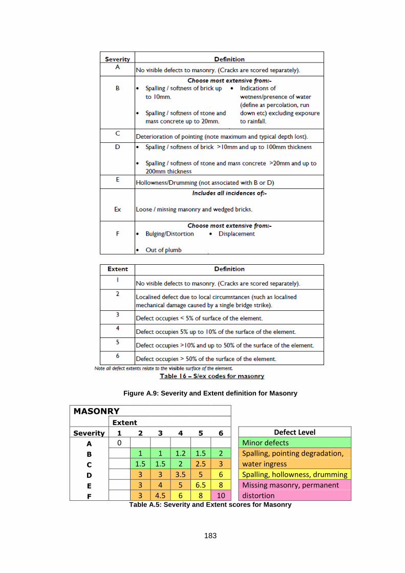
183
Figure A.9: Severity and Extent definition for Masonry
MASONRY Extent Severity 1 2 3 4 5 6
Defect Level
A 0
Minor defects
B 1 1 1.2 1.5 2
Spalling, pointing degradation,
C 1.5 1.5 2 2.5 3
water ingress
D 3 3 3.5 5 6
Spalling, hollowness, drumming
E 3 4 5 6.5 8
Missing masonry, permanent
F 3 4.5 6 8 10
distortion Table A.5: Severity and Extent scores for Masonry
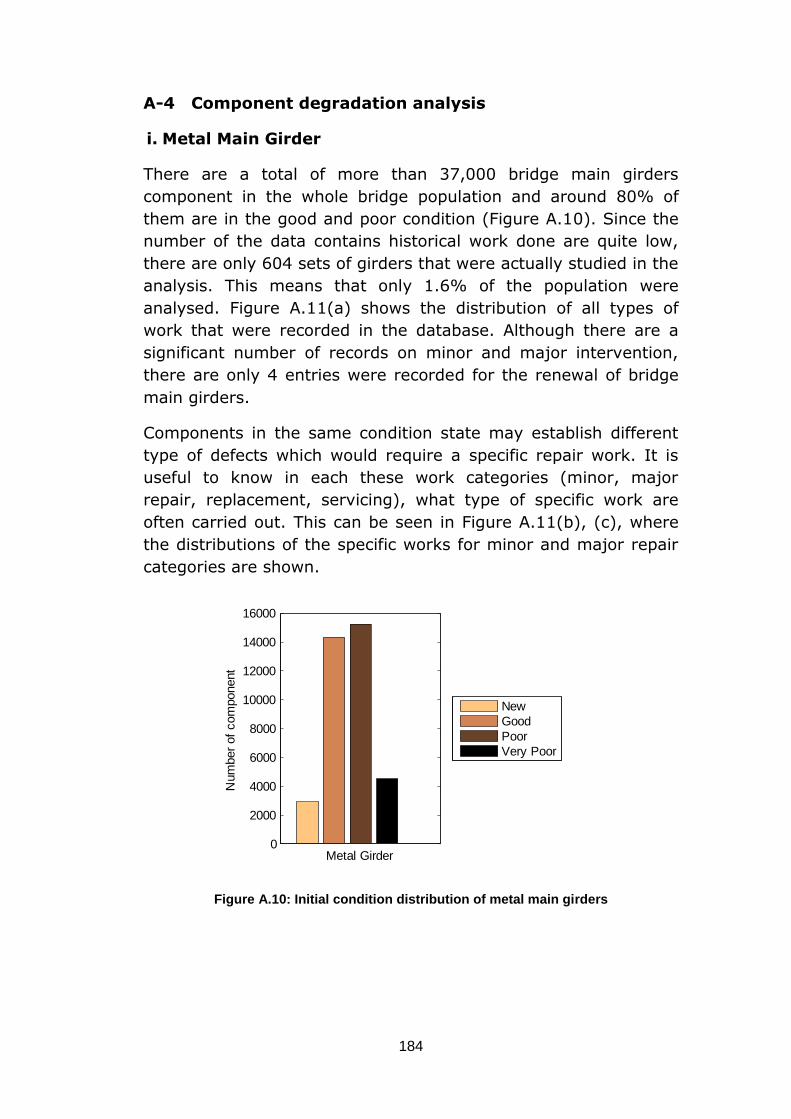
184
A-4 Component degradation analysis
i. Metal Main Girder
There are a total of more than 37,000 bridge main girders
component in the whole bridge population and around 80% of
them are in the good and poor condition (Figure A.10). Since the
number of the data contains historical work done are quite low,
there are only 604 sets of girders that were actually studied in the
analysis. This means that only 1.6% of the population were
analysed. Figure A.11(a) shows the distribution of all types of
work that were recorded in the database. Although there are a
significant number of records on minor and major intervention,
there are only 4 entries were recorded for the renewal of bridge
main girders.
Components in the same condition state may establish different
type of defects which would require a specific repair work. It is
useful to know in each these work categories (minor, major
repair, replacement, servicing), what type of specific work are
often carried out. This can be seen in Figure A.11(b), (c), where
the distributions of the specific works for minor and major repair
categories are shown.
Figure A.10: Initial condition distribution of metal main girders
0
2000
4000
6000
8000
10000
12000
14000
16000
Metal Girder
Num
ber
of
com
ponent
New
Good
Poor
Very Poor
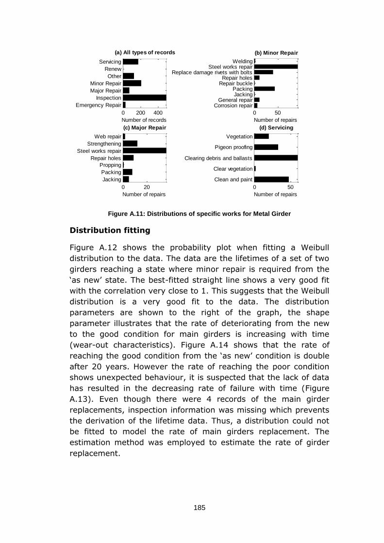
185
Figure A.11: Distributions of specific works for Metal Girder
Distribution fitting
Figure A.12 shows the probability plot when fitting a Weibull
distribution to the data. The data are the lifetimes of a set of two
girders reaching a state where minor repair is required from the
‘as new’ state. The best-fitted straight line shows a very good fit
with the correlation very close to 1. This suggests that the Weibull
distribution is a very good fit to the data. The distribution
parameters are shown to the right of the graph, the shape
parameter illustrates that the rate of deteriorating from the new
to the good condition for main girders is increasing with time
(wear-out characteristics). Figure A.14 shows that the rate of
reaching the good condition from the ‘as new’ condition is double
after 20 years. However the rate of reaching the poor condition
shows unexpected behaviour, it is suspected that the lack of data
has resulted in the decreasing rate of failure with time (Figure
A.13). Even though there were 4 records of the main girder
replacements, inspection information was missing which prevents
the derivation of the lifetime data. Thus, a distribution could not
be fitted to model the rate of main girders replacement. The
estimation method was employed to estimate the rate of girder
replacement.
0 200 400
Emergency Repair
Inspection
Major Repair
Minor Repair
Other
Renew
Servicing
Number of records
(a) All types of records
0 50
Corrosion repairGeneral repair
JackingPacking
Repair buckleRepair holes
Replace damage rivets with boltsSteel works repair
Welding
Number of repairs
(b) Minor Repair
0 20
Jacking
Packing
Propping
Repair holes
Steel works repair
Strengthening
Web repair
Number of repairs
(c) Major Repair
0 50
Clean and paint
Clear vegetation
Clearing debris and ballasts
Pigeon proofing
Vegetation
Number of repairs
(d) Servicing
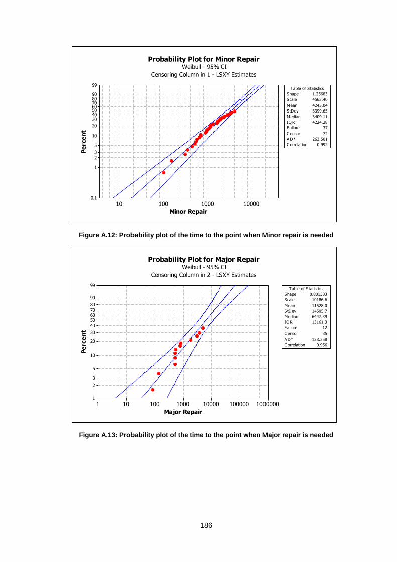
186
Figure A.12: Probability plot of the time to the point when Minor repair is needed
Figure A.13: Probability plot of the time to the point when Major repair is needed
10000100010010
99
90807060504030
20
10
5
32
1
0.1
Minor Repair
Pe
rce
nt
C orrelation 0.992
Shape 1.25683
Scale 4563.40
Mean 4245.04
StDev 3399.65
Median 3409.11
IQ R 4224.28
Failure 37
C ensor 72
A D* 263.501
Table of Statistics
Probability Plot for Minor Repair
Censoring Column in 1 - LSXY Estimates
Weibull - 95% CI
1000000100000100001000100101
99
90
8070605040
30
20
10
5
3
2
1
Major Repair
Pe
rce
nt
C orrelation 0.956
Shape 0.801303
Scale 10186.6
Mean 11528.0
StDev 14505.7
Median 6447.39
IQ R 13161.3
Failure 12
C ensor 35
A D* 128.358
Table of Statistics
Probability Plot for Major Repair
Censoring Column in 2 - LSXY Estimates
Weibull - 95% CI
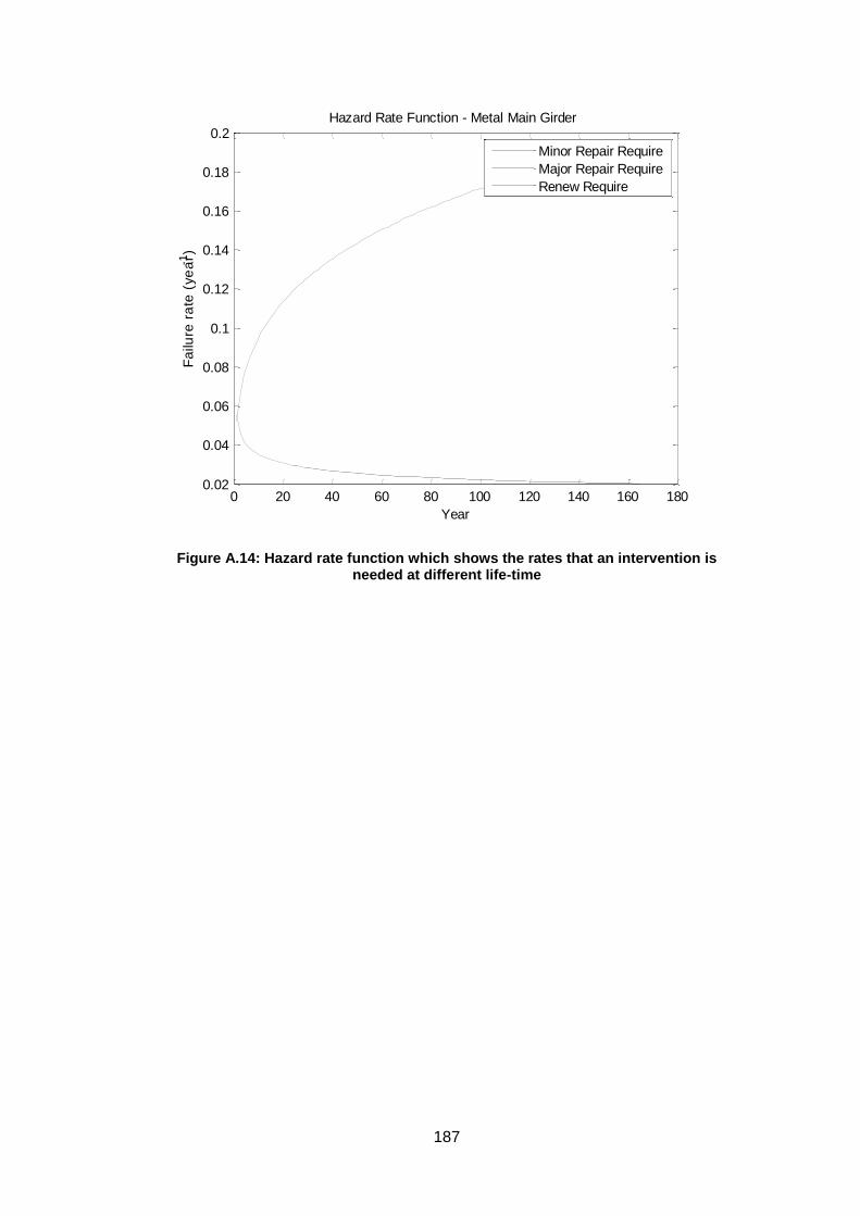
187
Figure A.14: Hazard rate function which shows the rates that an intervention is needed at different life-time
0 20 40 60 80 100 120 140 160 1800.02
0.04
0.06
0.08
0.1
0.12
0.14
0.16
0.18
0.2
Year
Fa
ilure
ra
te (
ye
ar-1)
Hazard Rate Function - Metal Main Girder
Minor Repair Require
Major Repair Require
Renew Require
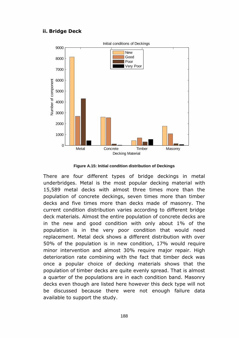
188
ii. Bridge Deck
Figure A.15: Initial condition distribution of Deckings
There are four different types of bridge deckings in metal
underbridges. Metal is the most popular decking material with
15,589 metal decks with almost three times more than the
population of concrete deckings, seven times more than timber
decks and five times more than decks made of masonry. The
current condition distribution varies according to different bridge
deck materials. Almost the entire population of concrete decks are
in the new and good condition with only about 1% of the
population is in the very poor condition that would need
replacement. Metal deck shows a different distribution with over
50% of the population is in new condition, 17% would require
minor intervention and almost 30% require major repair. High
deterioration rate combining with the fact that timber deck was
once a popular choice of decking materials shows that the
population of timber decks are quite evenly spread. That is almost
a quarter of the populations are in each condition band. Masonry
decks even though are listed here however this deck type will not
be discussed because there were not enough failure data
available to support the study.
Metal Concrete Timber Masonry0
1000
2000
3000
4000
5000
6000
7000
8000
9000
Decking Material
Num
ber
of
com
ponent
Initial conditions of Deckings
New
Good
Poor
Very Poor
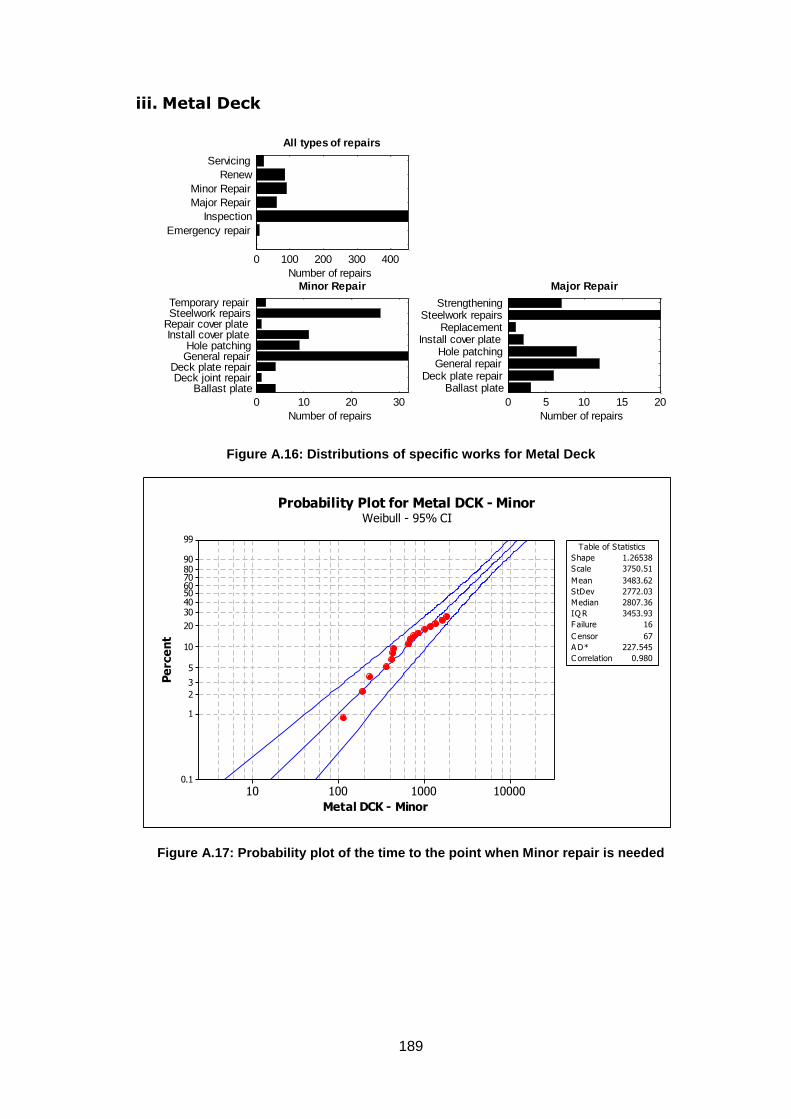
189
iii. Metal Deck
Figure A.16: Distributions of specific works for Metal Deck
Figure A.17: Probability plot of the time to the point when Minor repair is needed
0 100 200 300 400
Emergency repair
Inspection
Major Repair
Minor Repair
Renew
Servicing
Number of repairs
All types of repairs
0 10 20 30
Ballast plateDeck joint repair
Deck plate repairGeneral repairHole patching
Install cover plateRepair cover plateSteelwork repairsTemporary repair
Number of repairs
Minor Repair
0 5 10 15 20
Ballast plateDeck plate repair
General repairHole patching
Install cover plateReplacement
Steelwork repairsStrengthening
Number of repairs
Major Repair
10000100010010
99
90807060504030
20
10
5
3
2
1
0.1
Metal DCK - Minor
Pe
rce
nt
C orrelation 0.980
Shape 1.26538
Scale 3750.51
Mean 3483.62
StDev 2772.03
Median 2807.36
IQ R 3453.93
Failure 16
C ensor 67
A D* 227.545
Table of Statistics
Probability Plot for Metal DCK - MinorWeibull - 95% CI
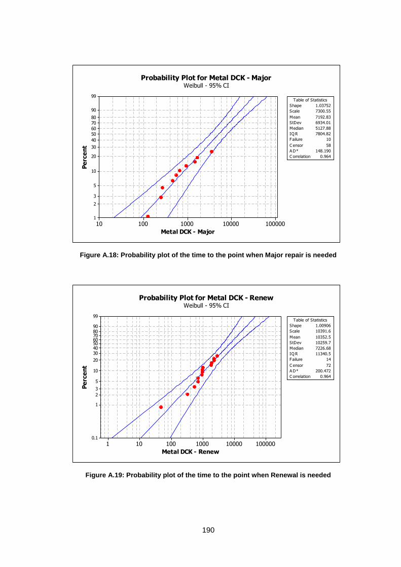
190
Figure A.18: Probability plot of the time to the point when Major repair is needed
Figure A.19: Probability plot of the time to the point when Renewal is needed
10000010000100010010
99
90
80706050
40
30
20
10
5
3
2
1
Metal DCK - Major
Pe
rce
nt
C orrelation 0.964
Shape 1.03752
Scale 7300.55
Mean 7192.83
StDev 6934.01
Median 5127.88
IQ R 7804.82
Failure 10
C ensor 58
A D* 148.190
Table of Statistics
Probability Plot for Metal DCK - MajorWeibull - 95% CI
100000100001000100101
99
90807060504030
20
10
5
3
2
1
0.1
Metal DCK - Renew
Pe
rce
nt
C orrelation 0.964
Shape 1.00906
Scale 10391.6
Mean 10352.5
StDev 10259.7
Median 7226.68
IQ R 11340.5
Failure 14
C ensor 72
A D* 200.472
Table of Statistics
Probability Plot for Metal DCK - RenewWeibull - 95% CI
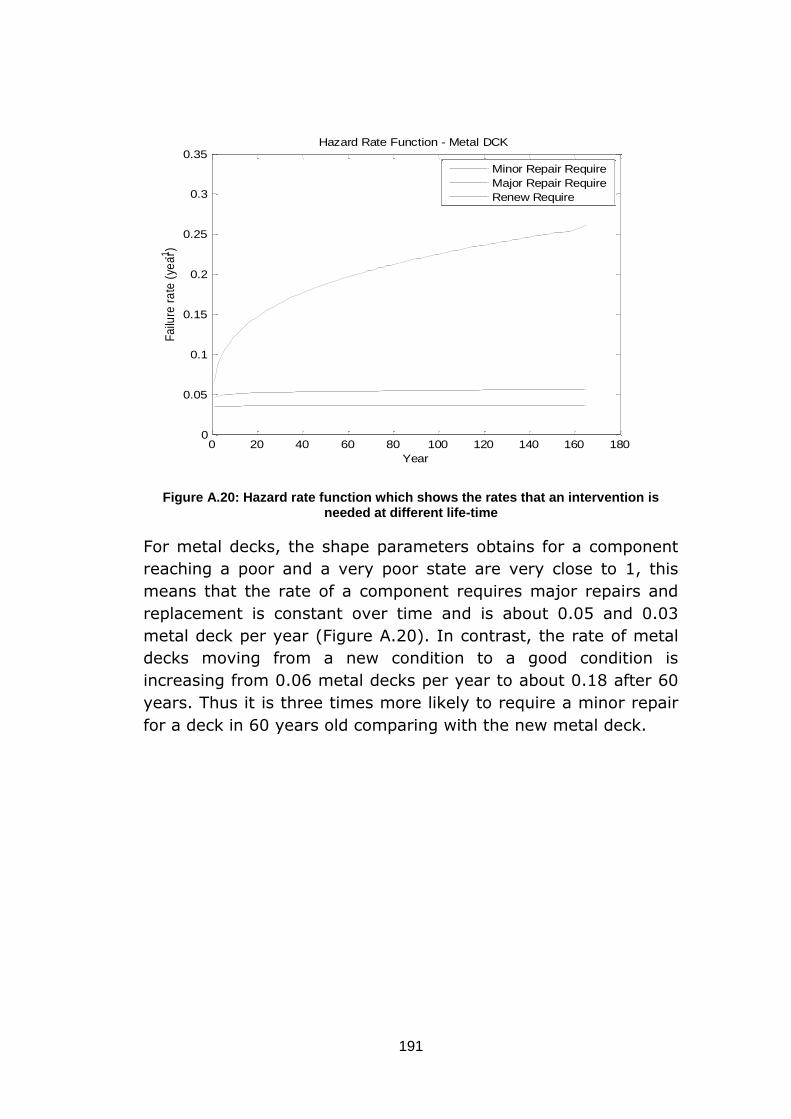
191
Figure A.20: Hazard rate function which shows the rates that an intervention is needed at different life-time
For metal decks, the shape parameters obtains for a component
reaching a poor and a very poor state are very close to 1, this
means that the rate of a component requires major repairs and
replacement is constant over time and is about 0.05 and 0.03
metal deck per year (Figure A.20). In contrast, the rate of metal
decks moving from a new condition to a good condition is
increasing from 0.06 metal decks per year to about 0.18 after 60
years. Thus it is three times more likely to require a minor repair
for a deck in 60 years old comparing with the new metal deck.
0 20 40 60 80 100 120 140 160 1800
0.05
0.1
0.15
0.2
0.25
0.3
0.35
Year
Fa
ilure
ra
te (
yea
r-1)
Hazard Rate Function - Metal DCK
Minor Repair Require
Major Repair Require
Renew Require
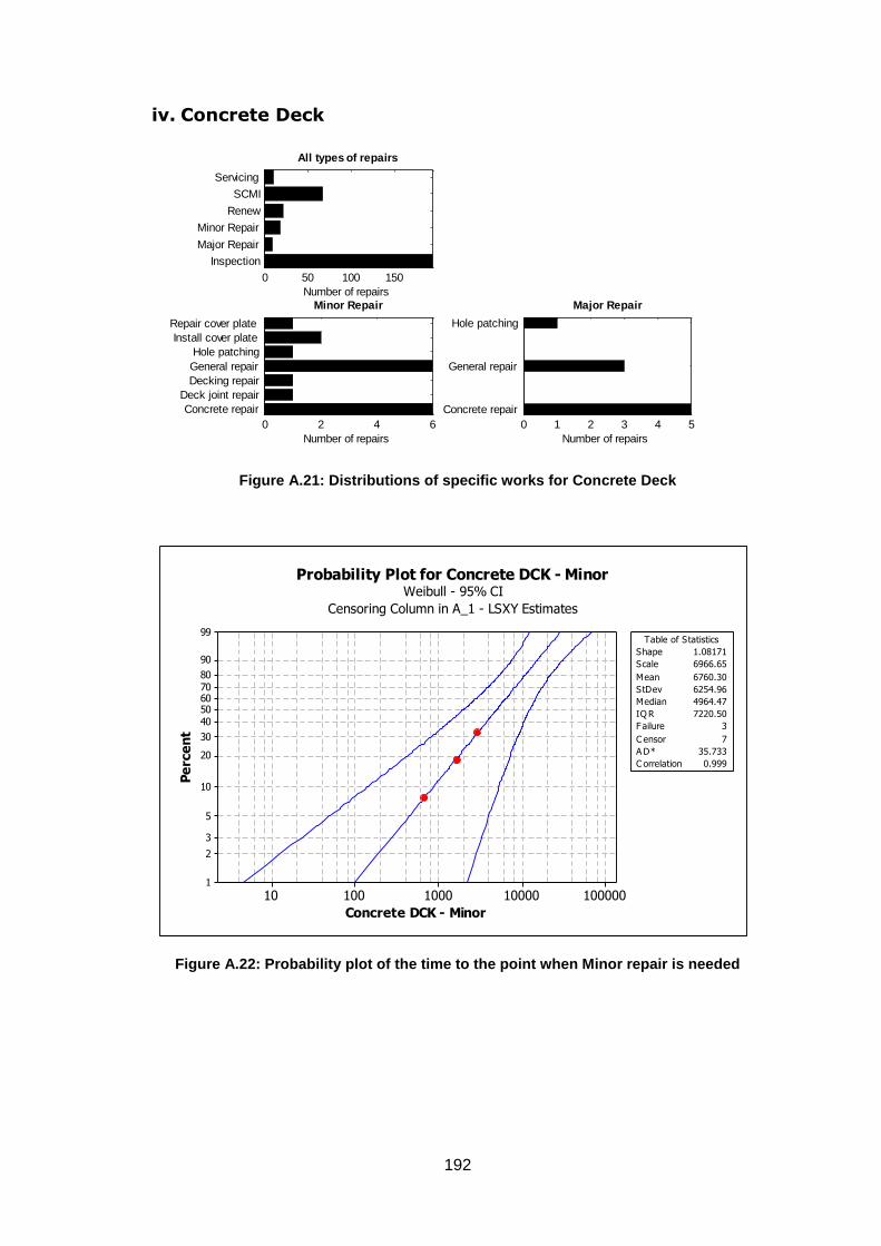
192
iv. Concrete Deck
Figure A.21: Distributions of specific works for Concrete Deck
Figure A.22: Probability plot of the time to the point when Minor repair is needed
0 50 100 150
Inspection
Major Repair
Minor Repair
Renew
SCMI
Servicing
Number of repairs
All types of repairs
0 2 4 6
Concrete repair
Deck joint repair
Decking repair
General repair
Hole patching
Install cover plate
Repair cover plate
Number of repairs
Minor Repair
0 1 2 3 4 5
Concrete repair
General repair
Hole patching
Number of repairs
Major Repair
10000010000100010010
99
90
8070605040
30
20
10
5
3
2
1
Concrete DCK - Minor
Pe
rce
nt
C orrelation 0.999
Shape 1.08171
Scale 6966.65
Mean 6760.30
StDev 6254.96
Median 4964.47
IQ R 7220.50
Failure 3
C ensor 7
A D* 35.733
Table of Statistics
Probability Plot for Concrete DCK - Minor
Censoring Column in A_1 - LSXY Estimates
Weibull - 95% CI
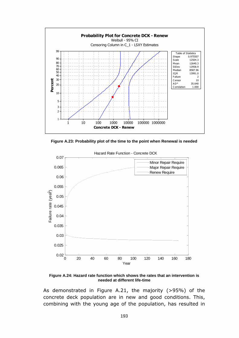
193
Figure A.23: Probability plot of the time to the point when Renewal is needed
Figure A.24: Hazard rate function which shows the rates that an intervention is needed at different life-time
As demonstrated in Figure A.21, the majority (>95%) of the
concrete deck population are in new and good conditions. This,
combining with the young age of the population, has resulted in
1000000100000100001000100101
99
90
8070605040
30
20
10
5
3
2
1
Concrete DCK - Renew
Pe
rce
nt
C orrelation 1.000
Shape 0.975507
Scale 12504.3
Mean 12640.3
StDev 12958.9
Median 8587.96
IQ R 13991.0
Failure 2
C ensor 10
A D* 35.640
Table of Statistics
Probability Plot for Concrete DCK - Renew
Censoring Column in C_1 - LSXY Estimates
Weibull - 95% CI
0 20 40 60 80 100 120 140 160 1800.02
0.025
0.03
0.035
0.04
0.045
0.05
0.055
0.06
0.065
0.07
Year
Fa
ilure
ra
te (
ye
ar-1)
Hazard Rate Function - Concrete DCK
Minor Repair Require
Major Repair Require
Renew Require
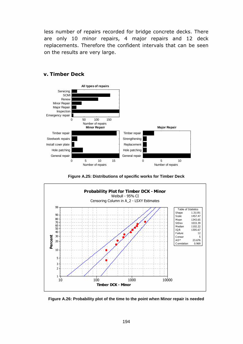
194
less number of repairs recorded for bridge concrete decks. There
are only 10 minor repairs, 4 major repairs and 12 deck
replacements. Therefore the confident intervals that can be seen
on the results are very large.
v. Timber Deck
Figure A.25: Distributions of specific works for Timber Deck
Figure A.26: Probability plot of the time to the point when Minor repair is needed
0 50 100 150
Emergency repair
Inspection
Major Repair
Minor Repair
Renew
SCMI
Servicing
Number of repairs
All types of repairs
0 5 10 15
General repair
Hole patching
Install cover plate
Steelwork repairs
Timber repair
Number of repairs
Minor Repair
0 5 10
General repair
Hole patching
Replacement
Strengthening
Timber repair
Number of repairs
Major Repair
10000100010010
99
90
8070605040
30
20
10
5
3
2
1
Timber DCK - Minor
Pe
rce
nt
C orrelation 0.969
Shape 1.31191
Scale 1457.47
Mean 1343.65
StDev 1033.39
Median 1102.22
IQ R 1305.67
Failure 12
C ensor 5
A D* 23.676
Table of Statistics
Probability Plot for Timber DCK - Minor
Censoring Column in A_2 - LSXY Estimates
Weibull - 95% CI
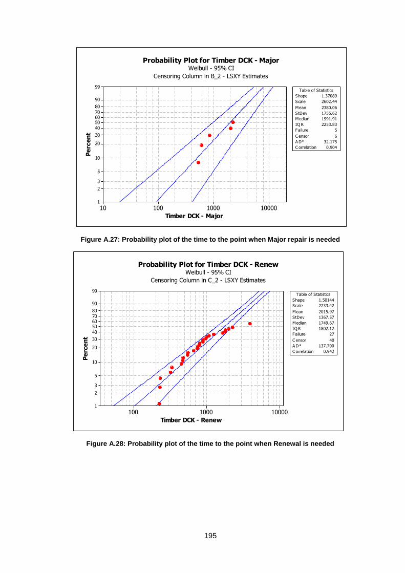
195
Figure A.27: Probability plot of the time to the point when Major repair is needed
Figure A.28: Probability plot of the time to the point when Renewal is needed
10000100010010
99
90
8070605040
30
20
10
5
3
2
1
Timber DCK - Major
Pe
rce
nt
C orrelation 0.904
Shape 1.37089
Scale 2602.44
Mean 2380.06
StDev 1756.62
Median 1991.91
IQ R 2253.83
Failure 5
C ensor 6
A D* 32.175
Table of Statistics
Probability Plot for Timber DCK - Major
Censoring Column in B_2 - LSXY Estimates
Weibull - 95% CI
100001000100
99
90
8070605040
30
20
10
5
3
2
1
Timber DCK - Renew
Pe
rce
nt
C orrelation 0.942
Shape 1.50144
Scale 2233.42
Mean 2015.97
StDev 1367.57
Median 1749.67
IQ R 1802.12
Failure 27
C ensor 40
A D* 137.700
Table of Statistics
Probability Plot for Timber DCK - Renew
Censoring Column in C_2 - LSXY Estimates
Weibull - 95% CI
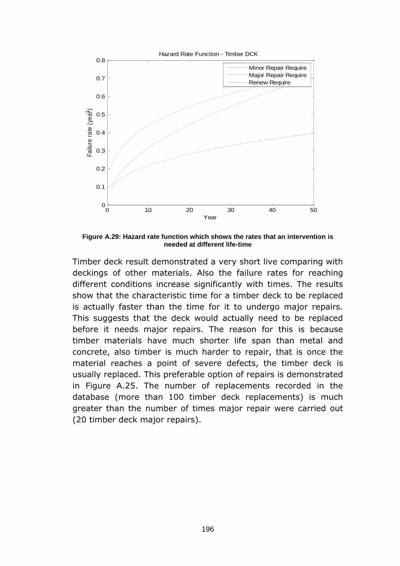
196
Figure A.29: Hazard rate function which shows the rates that an intervention is needed at different life-time
Timber deck result demonstrated a very short live comparing with
deckings of other materials. Also the failure rates for reaching
different conditions increase significantly with times. The results
show that the characteristic time for a timber deck to be replaced
is actually faster than the time for it to undergo major repairs.
This suggests that the deck would actually need to be replaced
before it needs major repairs. The reason for this is because
timber materials have much shorter life span than metal and
concrete, also timber is much harder to repair, that is once the
material reaches a point of severe defects, the timber deck is
usually replaced. This preferable option of repairs is demonstrated
in Figure A.25. The number of replacements recorded in the
database (more than 100 timber deck replacements) is much
greater than the number of times major repair were carried out
(20 timber deck major repairs).
0 10 20 30 40 500
0.1
0.2
0.3
0.4
0.5
0.6
0.7
0.8
Year
Fa
ilure
ra
te (
yea
r-1)
Hazard Rate Function - Timber DCK
Minor Repair Require
Major Repair Require
Renew Require
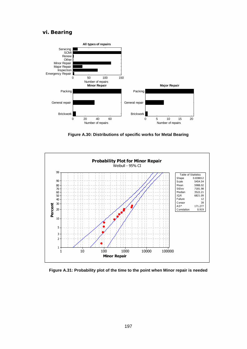
197
vi. Bearing
Figure A.30: Distributions of specific works for Metal Bearing
Figure A.31: Probability plot of the time to the point when Minor repair is needed
0 50 100 150
Emergency RepairInspection
Major RepairMinor Repair
OtherRenewSCMI
Servicing
Number of repairs
All types of repairs
0 20 40 60
Brickwork
General repair
Packing
Number of repairs
Minor Repair
0 5 10 15 20
Brickwork
General repair
Packing
Number of repairs
Major Repair
100000100001000100101
99
90
80706050
40
30
20
10
5
3
2
1
Minor Repair
Pe
rce
nt
C orrelation 0.919
Shape 0.838012
Scale 5454.54
Mean 5988.02
StDev 7181.98
Median 3522.21
IQ R 6821.09
Failure 12
C ensor 39
A D* 171.277
Table of Statistics
Probability Plot for Minor RepairWeibull - 95% CI
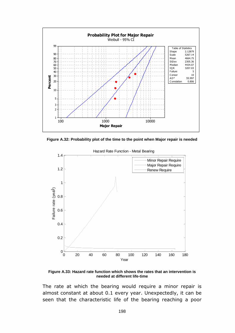
198
Figure A.32: Probability plot of the time to the point when Major repair is needed
Figure A.33: Hazard rate function which shows the rates that an intervention is needed at different life-time
The rate at which the bearing would require a minor repair is
almost constant at about 0.1 every year. Unexpectedly, it can be
seen that the characteristic life of the bearing reaching a poor
100001000100
99
90
80706050
40
30
20
10
5
3
2
1
Major Repair
Pe
rce
nt
C orrelation 0.806
Shape 2.12879
Scale 5267.14
Mean 4664.75
StDev 2305.36
Median 4434.07
IQ R 3207.03
Failure 5
C ensor 10
A D* 55.997
Table of Statistics
Probability Plot for Major RepairWeibull - 95% CI
0 20 40 60 80 100 120 140 160 1800
0.2
0.4
0.6
0.8
1
1.2
1.4
Year
Fa
ilure
ra
te (
ye
ar-1)
Hazard Rate Function - Metal Bearing
Minor Repair Require
Major Repair Require
Renew Require
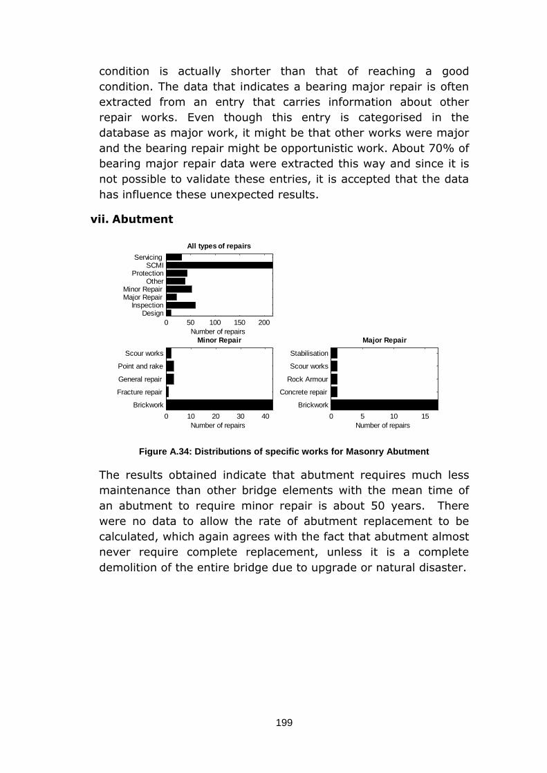
199
condition is actually shorter than that of reaching a good
condition. The data that indicates a bearing major repair is often
extracted from an entry that carries information about other
repair works. Even though this entry is categorised in the
database as major work, it might be that other works were major
and the bearing repair might be opportunistic work. About 70% of
bearing major repair data were extracted this way and since it is
not possible to validate these entries, it is accepted that the data
has influence these unexpected results.
vii. Abutment
Figure A.34: Distributions of specific works for Masonry Abutment
The results obtained indicate that abutment requires much less
maintenance than other bridge elements with the mean time of
an abutment to require minor repair is about 50 years. There
were no data to allow the rate of abutment replacement to be
calculated, which again agrees with the fact that abutment almost
never require complete replacement, unless it is a complete
demolition of the entire bridge due to upgrade or natural disaster.
0 50 100 150 200
DesignInspection
Major RepairMinor Repair
OtherProtection
SCMIServicing
Number of repairs
All types of repairs
0 10 20 30 40
Brickwork
Fracture repair
General repair
Point and rake
Scour works
Number of repairs
Minor Repair
0 5 10 15
Brickwork
Concrete repair
Rock Armour
Scour works
Stabilisation
Number of repairs
Major Repair
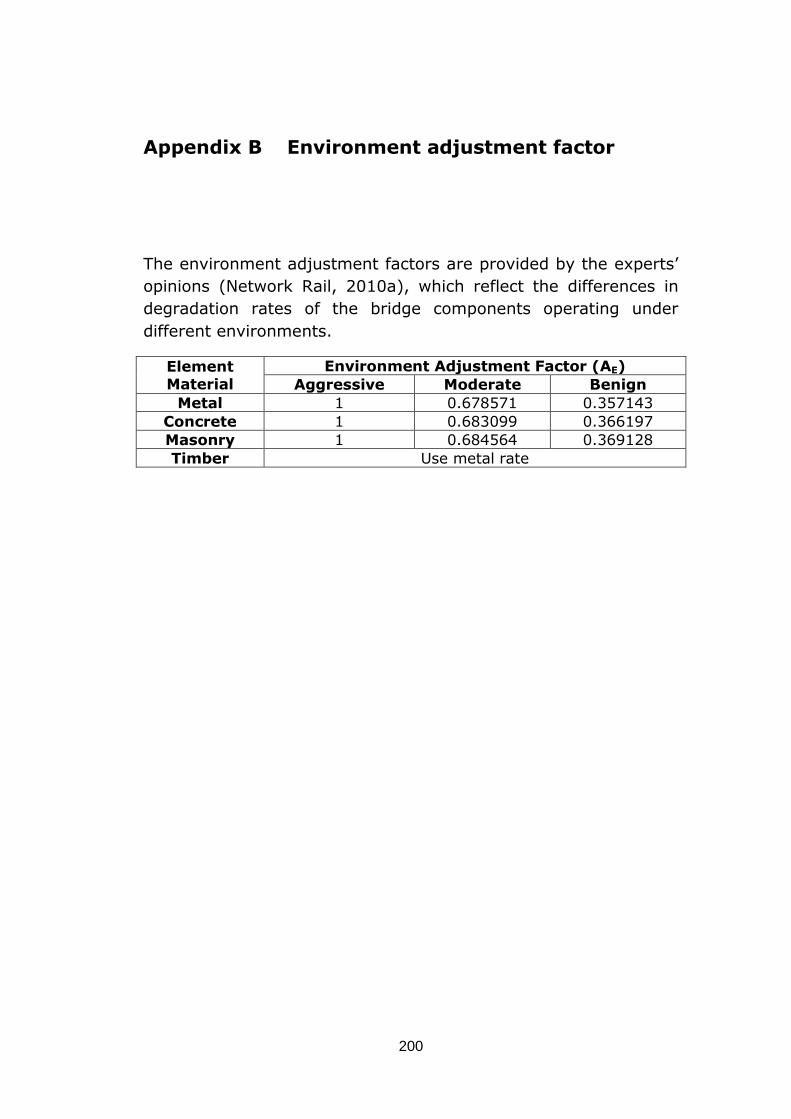
200
Appendix B Environment adjustment factor
The environment adjustment factors are provided by the experts’
opinions (Network Rail, 2010a), which reflect the differences in
degradation rates of the bridge components operating under
different environments.
Element Material
Environment Adjustment Factor (AE)
Aggressive Moderate Benign
Metal 1 0.678571 0.357143
Concrete 1 0.683099 0.366197
Masonry 1 0.684564 0.369128
Timber Use metal rate

201
Appendix C Markov bridge model
C-1 Transition rate matrix
The transition rate matrix for a bridge system contains two major
elements is a 32x32 matrix since there are 32 Markov states in
the model. The matrix is given below, where:
is the transition rate from the ‘as new’ state to the good state for component 1,
is the transition rate from the good state to the poor state for component 1,
is the transition rate from the poor state to the very poor state for component 1,
is the transition rate from the ‘as new’ state to the good state for component 2,
is the transition rate from the good state to the poor state for component 2,
is the transition rate from the poor state to the very poor state for component 2,
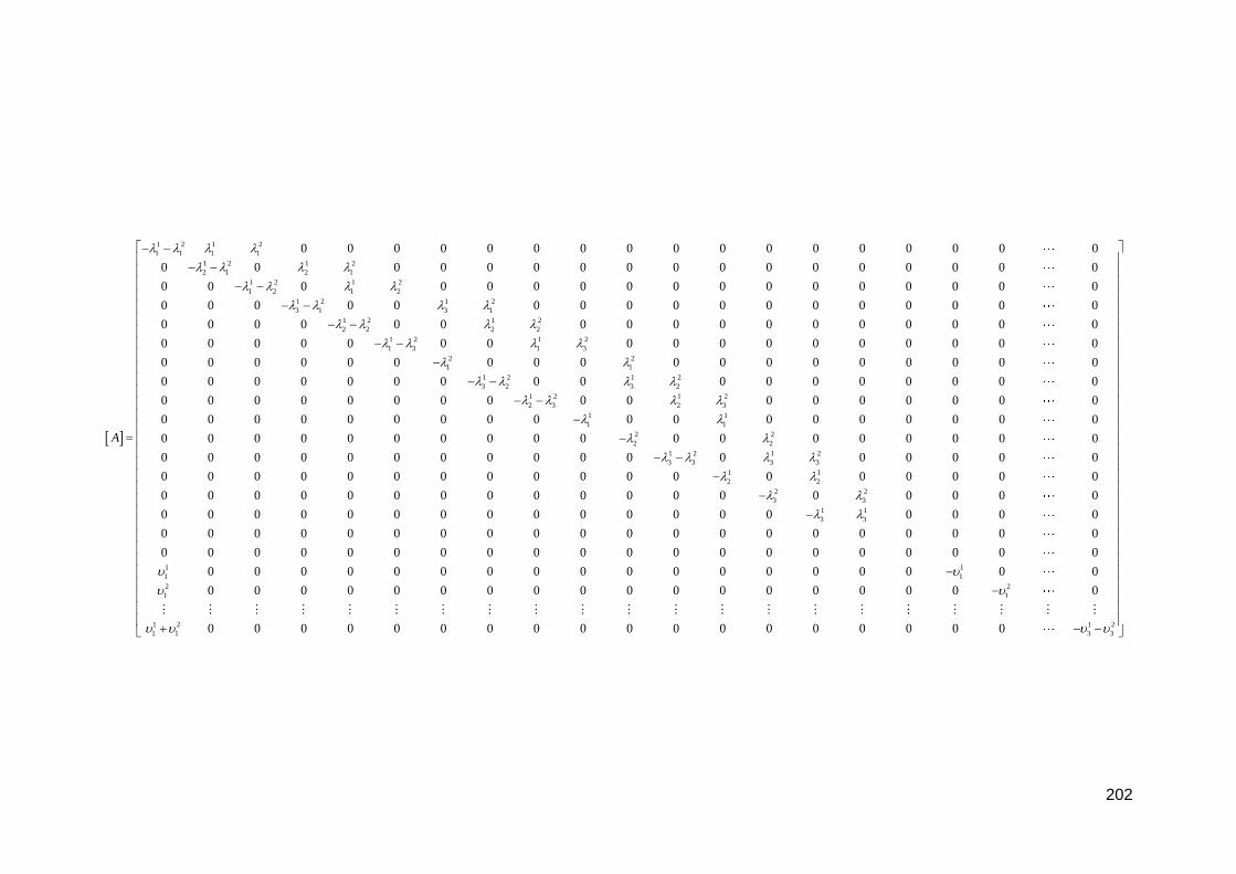
202
1 2 1 2
1 1 1 1
1 2 1 2
2 1 2 1
1 2 1 2
1 2 1 2
1 2 1 2
3 1 3 1
1 2 1 2
2 2 2 2
1 2 1 2
1 3 1 3
0 0 0 0 0 0 0 0 0 0 0 0 0 0 0 0 0
0 0 0 0 0 0 0 0 0 0 0 0 0 0 0 0 0
0 0 0 0 0 0 0 0 0 0 0 0 0 0 0 0 0
0 0 0 0 0 0 0 0 0 0 0 0 0 0 0 0 0
0 0 0 0 0 0 0 0 0 0 0 0 0 0 0 0 0
0 0 0 0 0 0 0 0 0 0 0 0 0 0 0 0 0
0 0 0 0 0 0
A
2 2
1 1
1 2 1 2
3 2 3 2
1 2 1 2
2 3 2 3
1 1
1 1
2 2
2 2
1 2 1 2
3 3 3 3
1 1
2 2
0 0 0 0 0 0 0 0 0 0 0 0
0 0 0 0 0 0 0 0 0 0 0 0 0 0 0 0 0
0 0 0 0 0 0 0 0 0 0 0 0 0 0 0 0 0
0 0 0 0 0 0 0 0 0 0 0 0 0 0 0 0 0 0
0 0 0 0 0 0 0 0 0 0 0 0 0 0 0 0 0 0
0 0 0 0 0 0 0 0 0 0 0 0 0 0 0 0 0
0 0 0 0 0 0 0 0 0 0 0 0 0 0 0 0 0 0
0 0 0 0 0 0
2 2
3 3
1 1
3 3
1 1
1 1
2 2
1 1
1 2 1 2
1 1 3 3
0 0 0 0 0 0 0 0 0 0 0 0
0 0 0 0 0 0 0 0 0 0 0 0 0 0 0 0 0 0
0 0 0 0 0 0 0 0 0 0 0 0 0 0 0 0 0 0 0 0
0 0 0 0 0 0 0 0 0 0 0 0 0 0 0 0 0 0 0 0
0 0 0 0 0 0 0 0 0 0 0 0 0 0 0 0 0 0
0 0 0 0 0 0 0 0 0 0 0 0 0 0 0 0 0 0
0 0 0 0 0 0 0 0 0 0 0 0 0 0 0 0 0 0
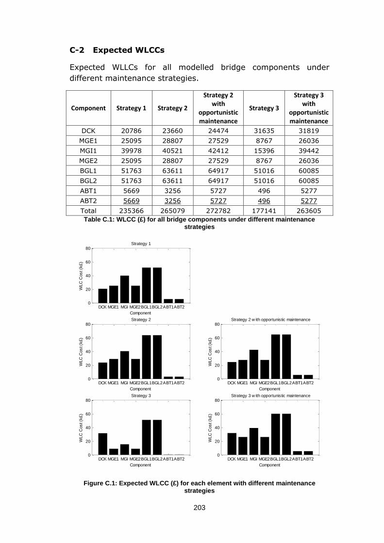
203
C-2 Expected WLCCs
Expected WLLCs for all modelled bridge components under
different maintenance strategies.
Component Strategy 1 Strategy 2
Strategy 2 with
opportunistic maintenance
Strategy 3
Strategy 3 with
opportunistic maintenance
DCK 20786 23660 24474 31635 31819
MGE1 25095 28807 27529 8767 26036
MGI1 39978 40521 42412 15396 39442
MGE2 25095 28807 27529 8767 26036
BGL1 51763 63611 64917 51016 60085
BGL2 51763 63611 64917 51016 60085
ABT1 5669 3256 5727 496 5277
ABT2 5669 3256 5727 496 5277
Total 235366 265079 272782 177141 263605
Table C.1: WLCC (£) for all bridge components under different maintenance strategies
Figure C.1: Expected WLCC (£) for each element with different maintenance strategies
DCK MGE1 MGI MGE2BGL1BGL2ABT1ABT20
20
40
60
80
Component
WLC
Cos
t (k
£)
Strategy 1
DCK MGE1 MGI MGE2BGL1BGL2ABT1ABT20
20
40
60
80
Component
WLC
Cos
t (k
£)
Strategy 2
DCK MGE1 MGI MGE2BGL1BGL2ABT1ABT20
20
40
60
80
Component
WLC
Cos
t (k
£)
Strategy 3
DCK MGE1 MGI MGE2BGL1BGL2ABT1ABT20
20
40
60
80
Component
WLC
Cos
t (k
£)
Strategy 2 w ith opportunistic maintenance
DCK MGE1 MGI MGE2BGL1BGL2ABT1ABT20
20
40
60
80
Component
WLC
Cos
t (k
£)
Strategy 3 w ith opportunistic maintenance
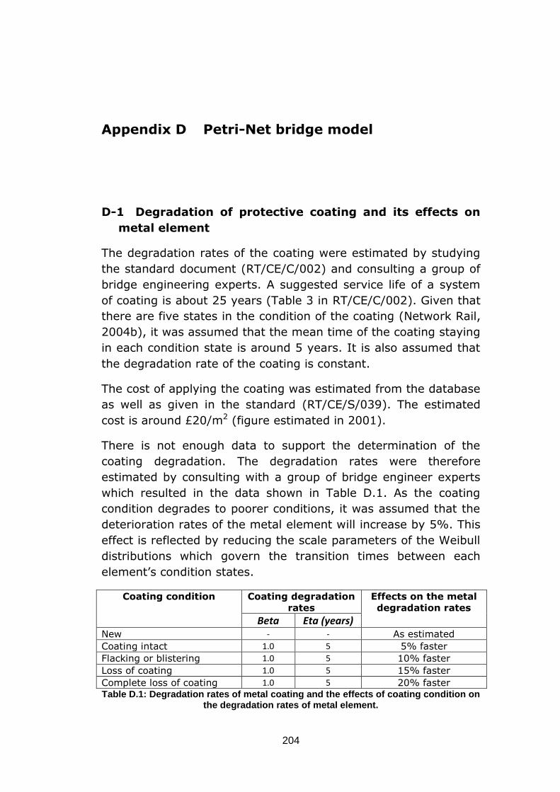
204
Appendix D Petri-Net bridge model
D-1 Degradation of protective coating and its effects on
metal element
The degradation rates of the coating were estimated by studying
the standard document (RT/CE/C/002) and consulting a group of
bridge engineering experts. A suggested service life of a system
of coating is about 25 years (Table 3 in RT/CE/C/002). Given that
there are five states in the condition of the coating (Network Rail,
2004b), it was assumed that the mean time of the coating staying
in each condition state is around 5 years. It is also assumed that
the degradation rate of the coating is constant.
The cost of applying the coating was estimated from the database
as well as given in the standard (RT/CE/S/039). The estimated
cost is around £20/m2 (figure estimated in 2001).
There is not enough data to support the determination of the
coating degradation. The degradation rates were therefore
estimated by consulting with a group of bridge engineer experts
which resulted in the data shown in Table D.1. As the coating
condition degrades to poorer conditions, it was assumed that the
deterioration rates of the metal element will increase by 5%. This
effect is reflected by reducing the scale parameters of the Weibull
distributions which govern the transition times between each
element’s condition states.
Coating condition Coating degradation
rates
Effects on the metal
degradation rates
Beta Eta (years) New - - As estimated
Coating intact 1.0 5 5% faster
Flacking or blistering 1.0 5 10% faster
Loss of coating 1.0 5 15% faster
Complete loss of coating 1.0 5 20% faster Table D.1: Degradation rates of metal coating and the effects of coating condition on
the degradation rates of metal element.
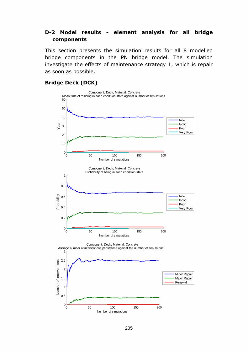
205
D-2 Model results - element analysis for all bridge
components
This section presents the simulation results for all 8 modelled
bridge components in the PN bridge model. The simulation
investigate the effects of maintenance strategy 1, which is repair
as soon as possible.
Bridge Deck (DCK)
0 50 100 150 2000
10
20
30
40
50
60
Number of simulations
Ye
ar
Component: Deck, Material: ConcreteMean time of residing in each condition state against number of simulations
New
Good
Poor
Very Poor
0 50 100 150 2000
0.2
0.4
0.6
0.8
1
Number of simulations
Pro
ba
bili
ty
Component: Deck, Material: ConcreteProbability of being in each condition state
New
Good
Poor
Very Poor
0 50 100 150 2000
0.5
1
1.5
2
2.5
3
Number of simulations
Nu
mb
er
of
inte
rve
ntio
ns
Component: Deck, Material: ConcreteAverage number of interventions per lifetime against the number of simulatons
Minor Repair
Major Repair
Renewal
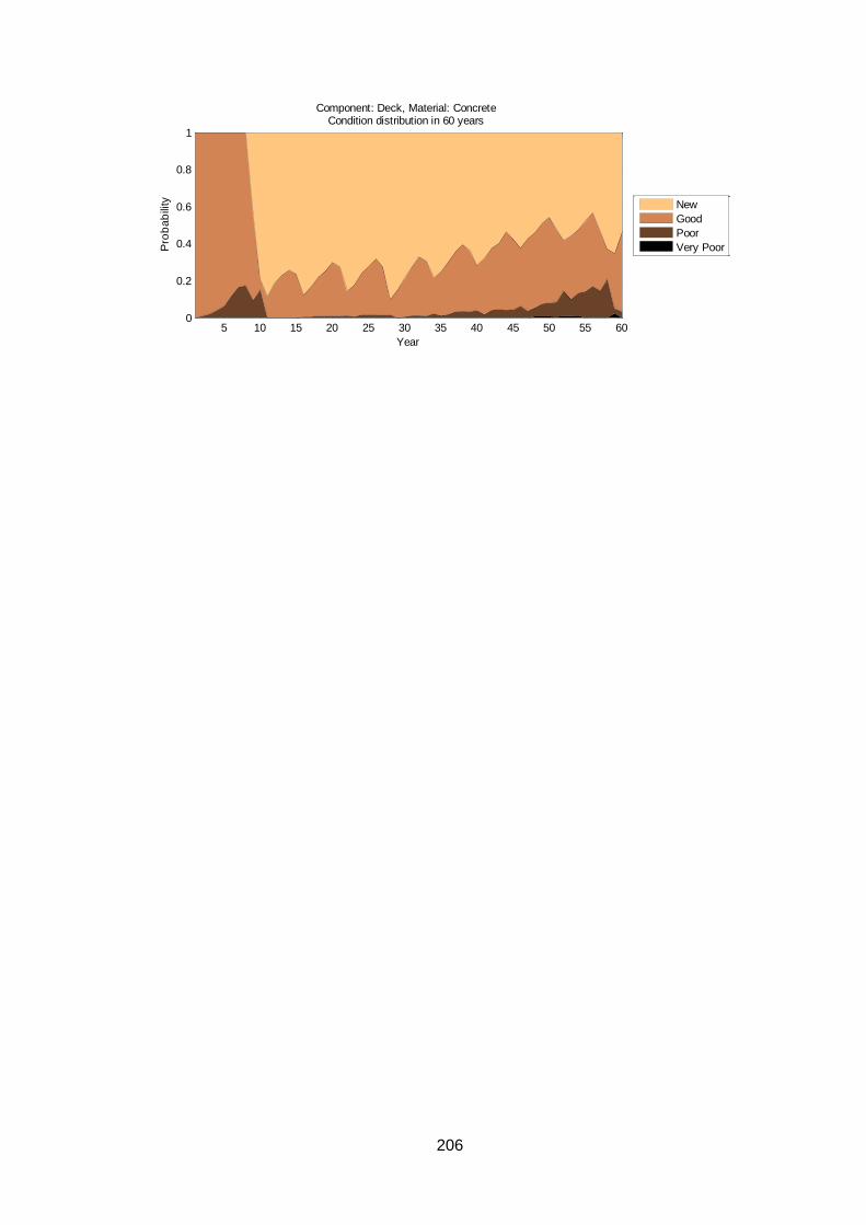
206
5 10 15 20 25 30 35 40 45 50 55 600
0.2
0.4
0.6
0.8
1
Year
Pro
ba
bili
ty
Component: Deck, Material: ConcreteCondition distribution in 60 years
New
Good
Poor
Very Poor

207
External Main Girder 1 (MGE1)
0 50 100 150 2000
10
20
30
40
50
Number of simulations
Ye
ar
Component: Girder, Material: MetalMean time of residing in each condition state against number of simulations
New
Good
Poor
Very Poor
0 50 100 150 2000
0.2
0.4
0.6
0.8
1
Number of simulations
Pro
ba
bili
ty
Component: Girder, Material: MetalProbability of being in each condition state
New
Good
Poor
Very Poor
0 50 100 150 2000
0.5
1
1.5
2
2.5
3
Number of simulations
Nu
mb
er
of
inte
rve
ntio
ns
Component: Girder, Material: MetalAverage number of interventions per lifetime against the number of simulatons
Minor Repair
Major Repair
Renewal
5 10 15 20 25 30 35 40 45 50 55 600
0.2
0.4
0.6
0.8
1
Year
Pro
ba
bili
ty
Component: Girder, Material: MetalCondition distribution in 60 years
New
Good
Poor
Very Poor

208
Internal Main Girder (MGI)
0 50 100 150 2000
10
20
30
40
50
Number of simulations
Ye
ar
Component: Girder, Material: MetalMean time of residing in each condition state against number of simulations
New
Good
Poor
Very Poor
0 50 100 150 2000
0.2
0.4
0.6
0.8
1
Number of simulations
Pro
ba
bili
ty
Component: Girder, Material: MetalProbability of being in each condition state
New
Good
Poor
Very Poor
0 50 100 150 2000
0.5
1
1.5
2
2.5
3
Number of simulations
Nu
mb
er
of
inte
rve
ntio
ns
Component: Girder, Material: MetalAverage number of interventions per lifetime against the number of simulatons
Minor Repair
Major Repair
Renewal
5 10 15 20 25 30 35 40 45 50 55 600
0.2
0.4
0.6
0.8
1
Year
Pro
ba
bili
ty
Component: Girder, Material: MetalCondition distribution in 60 years
New
Good
Poor
Very Poor
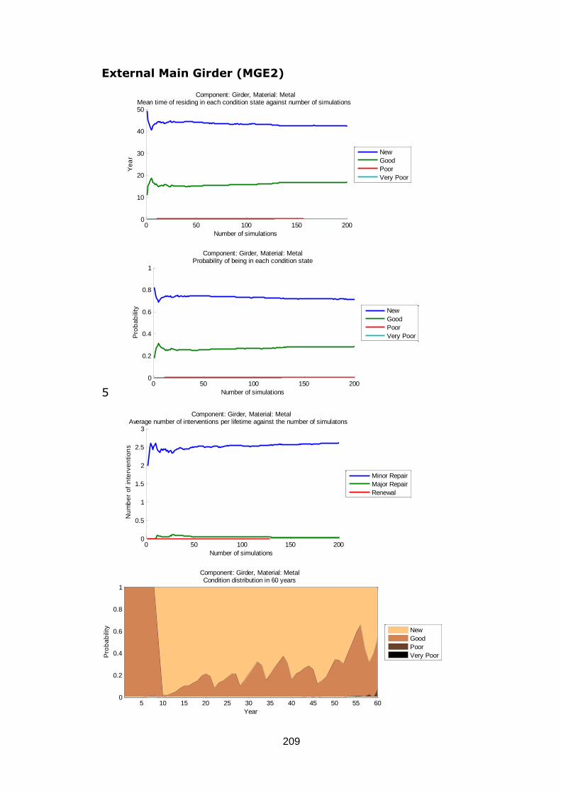
209
External Main Girder (MGE2)
5
0 50 100 150 2000
10
20
30
40
50
Number of simulations
Ye
ar
Component: Girder, Material: MetalMean time of residing in each condition state against number of simulations
New
Good
Poor
Very Poor
0 50 100 150 2000
0.2
0.4
0.6
0.8
1
Number of simulations
Pro
ba
bili
ty
Component: Girder, Material: MetalProbability of being in each condition state
New
Good
Poor
Very Poor
0 50 100 150 2000
0.5
1
1.5
2
2.5
3
Number of simulations
Nu
mb
er
of
inte
rve
ntio
ns
Component: Girder, Material: MetalAverage number of interventions per lifetime against the number of simulatons
Minor Repair
Major Repair
Renewal
5 10 15 20 25 30 35 40 45 50 55 600
0.2
0.4
0.6
0.8
1
Year
Pro
ba
bili
ty
Component: Girder, Material: MetalCondition distribution in 60 years
New
Good
Poor
Very Poor

210
Bearing 1 (BGL1)
0 50 100 150 2000
5
10
15
20
25
30
35
40
Number of simulations
Ye
ar
Component: Bearing, Material: MetalMean time of residing in each condition state against number of simulations
New
Good
Poor
Very Poor
0 50 100 150 2000
0.2
0.4
0.6
0.8
1
Number of simulations
Pro
ba
bili
ty
Component: Bearing, Material: MetalProbability of being in each condition state
New
Good
Poor
Very Poor
0 50 100 150 2000
0.5
1
1.5
2
2.5
3
Number of simulations
Nu
mb
er
of
inte
rve
ntio
ns
Component: Bearing, Material: MetalAverage number of interventions per lifetime against the number of simulatons
Minor Repair
Major Repair
Renewal
5 10 15 20 25 30 35 40 45 50 55 600
0.2
0.4
0.6
0.8
1
Year
Pro
ba
bili
ty
Component: Bearing, Material: MetalCondition distribution in 60 years
New
Good
Poor
Very Poor
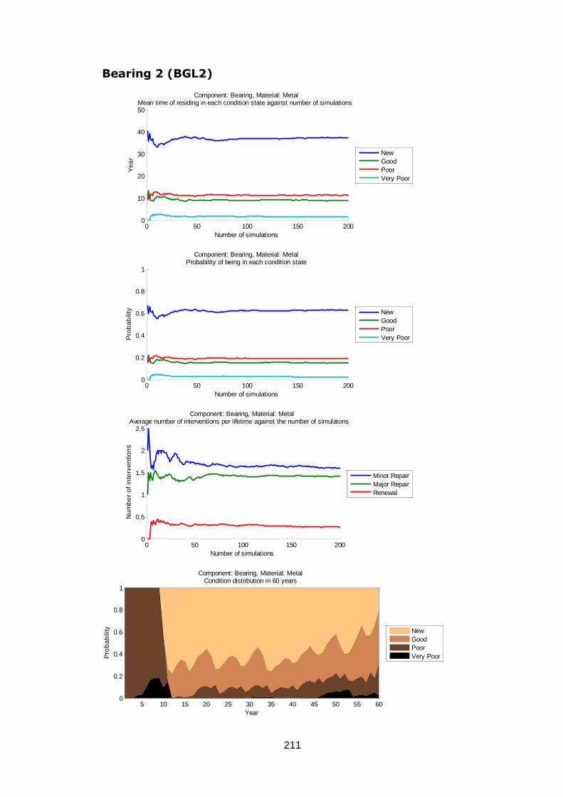
211
Bearing 2 (BGL2)
0 50 100 150 2000
10
20
30
40
50
Number of simulations
Ye
ar
Component: Bearing, Material: MetalMean time of residing in each condition state against number of simulations
New
Good
Poor
Very Poor
0 50 100 150 2000
0.2
0.4
0.6
0.8
1
Number of simulations
Pro
ba
bili
ty
Component: Bearing, Material: MetalProbability of being in each condition state
New
Good
Poor
Very Poor
0 50 100 150 2000
0.5
1
1.5
2
2.5
Number of simulations
Nu
mb
er
of
inte
rve
ntio
ns
Component: Bearing, Material: MetalAverage number of interventions per lifetime against the number of simulatons
Minor Repair
Major Repair
Renewal
5 10 15 20 25 30 35 40 45 50 55 600
0.2
0.4
0.6
0.8
1
Year
Pro
ba
bili
ty
Component: Bearing, Material: MetalCondition distribution in 60 years
New
Good
Poor
Very Poor
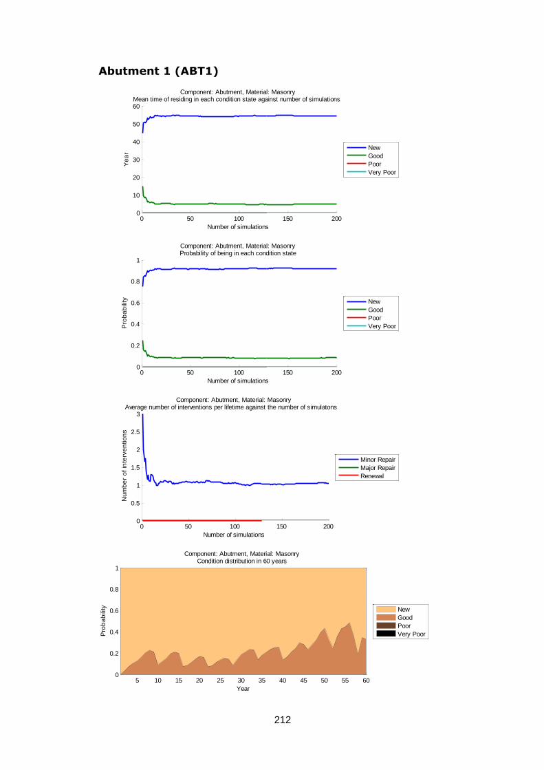
212
Abutment 1 (ABT1)
0 50 100 150 2000
10
20
30
40
50
60
Number of simulations
Ye
ar
Component: Abutment, Material: MasonryMean time of residing in each condition state against number of simulations
New
Good
Poor
Very Poor
0 50 100 150 2000
0.2
0.4
0.6
0.8
1
Number of simulations
Pro
ba
bili
ty
Component: Abutment, Material: MasonryProbability of being in each condition state
New
Good
Poor
Very Poor
0 50 100 150 2000
0.5
1
1.5
2
2.5
3
Number of simulations
Nu
mb
er
of
inte
rve
ntio
ns
Component: Abutment, Material: MasonryAverage number of interventions per lifetime against the number of simulatons
Minor Repair
Major Repair
Renewal
5 10 15 20 25 30 35 40 45 50 55 600
0.2
0.4
0.6
0.8
1
Year
Pro
ba
bili
ty
Component: Abutment, Material: MasonryCondition distribution in 60 years
New
Good
Poor
Very Poor
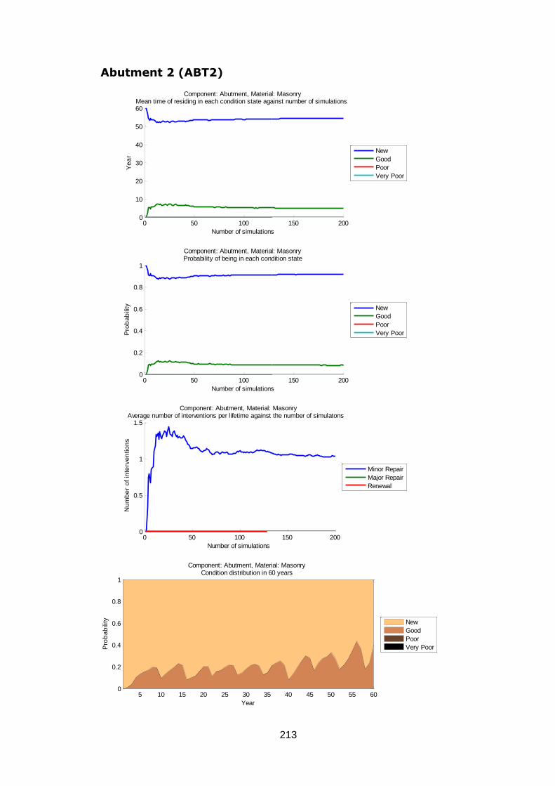
213
Abutment 2 (ABT2)
0 50 100 150 2000
10
20
30
40
50
60
Number of simulations
Ye
ar
Component: Abutment, Material: MasonryMean time of residing in each condition state against number of simulations
New
Good
Poor
Very Poor
0 50 100 150 2000
0.2
0.4
0.6
0.8
1
Number of simulations
Pro
ba
bili
ty
Component: Abutment, Material: MasonryProbability of being in each condition state
New
Good
Poor
Very Poor
0 50 100 150 2000
0.5
1
1.5
Number of simulations
Nu
mb
er
of
inte
rve
ntio
ns
Component: Abutment, Material: MasonryAverage number of interventions per lifetime against the number of simulatons
Minor Repair
Major Repair
Renewal
5 10 15 20 25 30 35 40 45 50 55 600
0.2
0.4
0.6
0.8
1
Year
Pro
ba
bili
ty
Component: Abutment, Material: MasonryCondition distribution in 60 years
New
Good
Poor
Very Poor
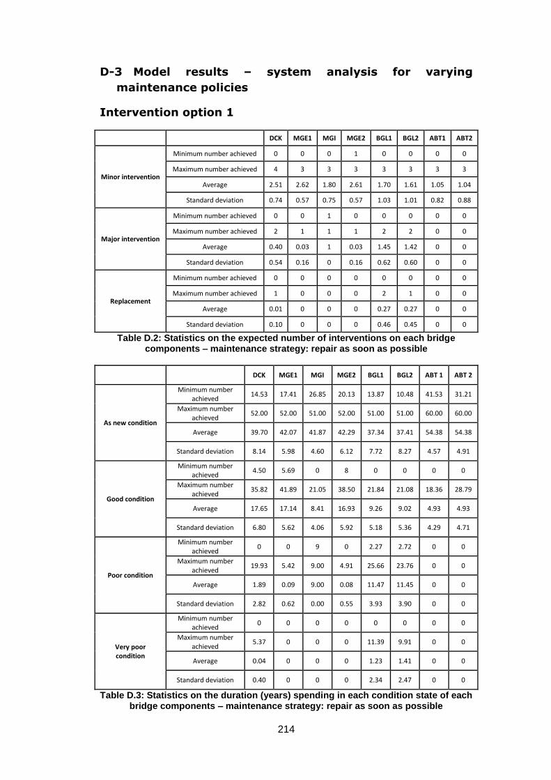
214
D-3 Model results – system analysis for varying
maintenance policies
Intervention option 1
DCK MGE1 MGI MGE2 BGL1 BGL2 ABT1 ABT2
Minor intervention
Minimum number achieved 0 0 0 1 0 0 0 0
Maximum number achieved 4 3 3 3 3 3 3 3
Average 2.51 2.62 1.80 2.61 1.70 1.61 1.05 1.04
Standard deviation 0.74 0.57 0.75 0.57 1.03 1.01 0.82 0.88
Major intervention
Minimum number achieved 0 0 1 0 0 0 0 0
Maximum number achieved 2 1 1 1 2 2 0 0
Average 0.40 0.03 1 0.03 1.45 1.42 0 0
Standard deviation 0.54 0.16 0 0.16 0.62 0.60 0 0
Replacement
Minimum number achieved 0 0 0 0 0 0 0 0
Maximum number achieved 1 0 0 0 2 1 0 0
Average 0.01 0 0 0 0.27 0.27 0 0
Standard deviation 0.10 0 0 0 0.46 0.45 0 0
Table D.2: Statistics on the expected number of interventions on each bridge components – maintenance strategy: repair as soon as possible
DCK MGE1 MGI MGE2 BGL1 BGL2 ABT 1 ABT 2
As new condition
Minimum number achieved
14.53 17.41 26.85 20.13 13.87 10.48 41.53 31.21
Maximum number achieved
52.00 52.00 51.00 52.00 51.00 51.00 60.00 60.00
Average 39.70 42.07 41.87 42.29 37.34 37.41 54.38 54.38
Standard deviation 8.14 5.98 4.60 6.12 7.72 8.27 4.57 4.91
Good condition
Minimum number achieved
4.50 5.69 0 8 0 0 0 0
Maximum number achieved
35.82 41.89 21.05 38.50 21.84 21.08 18.36 28.79
Average 17.65 17.14 8.41 16.93 9.26 9.02 4.93 4.93
Standard deviation 6.80 5.62 4.06 5.92 5.18 5.36 4.29 4.71
Poor condition
Minimum number achieved
0 0 9 0 2.27 2.72 0 0
Maximum number achieved
19.93 5.42 9.00 4.91 25.66 23.76 0 0
Average 1.89 0.09 9.00 0.08 11.47 11.45 0 0
Standard deviation 2.82 0.62 0.00 0.55 3.93 3.90 0 0
Very poor condition
Minimum number achieved
0 0 0 0 0 0 0 0
Maximum number achieved
5.37 0 0 0 11.39 9.91 0 0
Average 0.04 0 0 0 1.23 1.41 0 0
Standard deviation 0.40 0 0 0 2.34 2.47 0 0
Table D.3: Statistics on the duration (years) spending in each condition state of each bridge components – maintenance strategy: repair as soon as possible
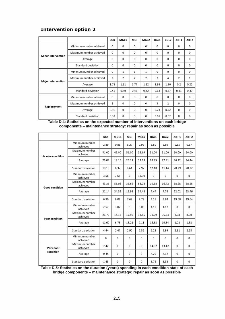
215
Intervention option 2
DCK MGE1 MGI MGE2 BGL1 BGL2 ABT1 ABT2
Minor intervention
Minimum number achieved 0 0 0 0 0 0 0 0
Maximum number achieved 0 0 0 0 0 0 0 0
Average 0 0 0 0 0 0 0 0
Standard deviation 0 0 0 0 0 0 0 0
Major intervention
Minimum number achieved 0 1 1 1 0 0 0 0
Maximum number achieved 2 2 2 2 3 4 2 1
Average 1.78 1.21 1.77 1.22 1.98 1.96 0.2 0.25
Standard deviation 0.45 0.40 0.43 0.42 0.64 0.57 0.41 0.43
Replacement
Minimum number achieved 0 0 0 0 0 0 0 0
Maximum number achieved 2 0 0 0 3 2 0 0
Average 0.10 0 0 0 0.73 0.72 0 0
Standard deviation 0.32 0 0 0 0.61 0.52 0 0
Table D.4: Statistics on the expected number of interventions on each bridge components – maintenance strategy: repair as soon as possible
DCK MGE1 MGI MGE2 BGL1 BGL2 ABT 1 ABT 2
As new condition
Minimum number achieved
2.89 0.85 6.27 0.99 3.50 6.69 0.55 0.37
Maximum number achieved
51.00 45.00 51.00 38.69 51.00 51.00 60.00 60.00
Average 26.03 18.16 26.11 17.63 28.85 27.81 36.22 34.44
Standard deviation 10.10 8.37 8.61 7.97 12.10 11.14 20.29 20.32
Good condition
Minimum number achieved
3.56 7.68 0 13.39 0 0 0 0
Maximum number achieved
43.36 55.08 36.65 53.08 19.68 16.72 58.28 58.55
Average 21.14 34.32 19.93 34.48 7.44 7.76 22.02 23.46
Standard deviation 6.90 8.08 7.69 7.79 4.18 3.84 19.58 19.04
Poor condition
Minimum number achieved
2.57 3.07 9 3.08 4.19 4.12 0 0
Maximum number achieved
26.79 14.14 17.96 14.55 31.09 35.83 8.98 8.90
Average 11.60 6.78 13.21 7.11 18.63 19.54 1.02 1.38
Standard deviation 4.44 2.47 2.90 2.36 6.21 5.99 2.31 2.58
Very poor condition
Minimum number achieved
0 0 0 0 0 0 0 0
Maximum number achieved
7.42 0 0 0 14.32 13.12 0 0
Average 0.45 0 0 0 4.29 4.12 0 0
Standard deviation 1.45 0 0 0 3.75 3.33 0 0
Table D.5: Statistics on the duration (years) spending in each condition state of each bridge components – maintenance strategy: repair as soon as possible
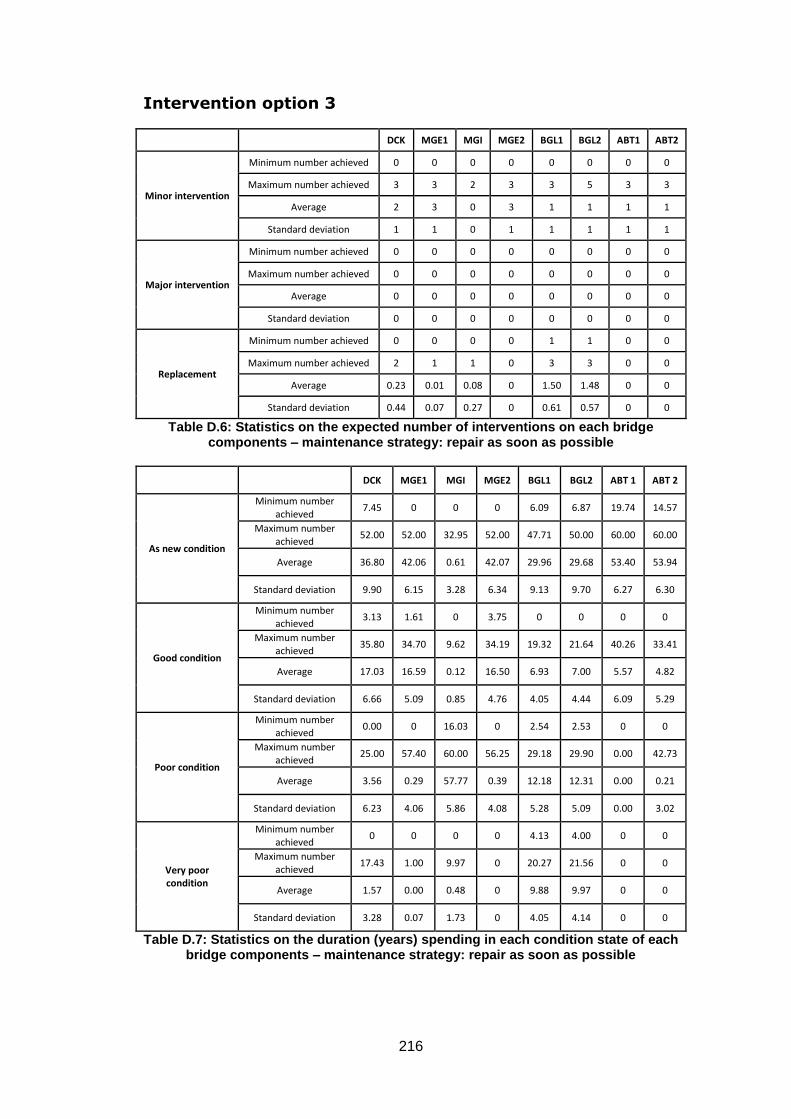
216
Intervention option 3
DCK MGE1 MGI MGE2 BGL1 BGL2 ABT1 ABT2
Minor intervention
Minimum number achieved 0 0 0 0 0 0 0 0
Maximum number achieved 3 3 2 3 3 5 3 3
Average 2 3 0 3 1 1 1 1
Standard deviation 1 1 0 1 1 1 1 1
Major intervention
Minimum number achieved 0 0 0 0 0 0 0 0
Maximum number achieved 0 0 0 0 0 0 0 0
Average 0 0 0 0 0 0 0 0
Standard deviation 0 0 0 0 0 0 0 0
Replacement
Minimum number achieved 0 0 0 0 1 1 0 0
Maximum number achieved 2 1 1 0 3 3 0 0
Average 0.23 0.01 0.08 0 1.50 1.48 0 0
Standard deviation 0.44 0.07 0.27 0 0.61 0.57 0 0
Table D.6: Statistics on the expected number of interventions on each bridge components – maintenance strategy: repair as soon as possible
DCK MGE1 MGI MGE2 BGL1 BGL2 ABT 1 ABT 2
As new condition
Minimum number achieved
7.45 0 0 0 6.09 6.87 19.74 14.57
Maximum number achieved
52.00 52.00 32.95 52.00 47.71 50.00 60.00 60.00
Average 36.80 42.06 0.61 42.07 29.96 29.68 53.40 53.94
Standard deviation 9.90 6.15 3.28 6.34 9.13 9.70 6.27 6.30
Good condition
Minimum number achieved
3.13 1.61 0 3.75 0 0 0 0
Maximum number achieved
35.80 34.70 9.62 34.19 19.32 21.64 40.26 33.41
Average 17.03 16.59 0.12 16.50 6.93 7.00 5.57 4.82
Standard deviation 6.66 5.09 0.85 4.76 4.05 4.44 6.09 5.29
Poor condition
Minimum number achieved
0.00 0 16.03 0 2.54 2.53 0 0
Maximum number achieved
25.00 57.40 60.00 56.25 29.18 29.90 0.00 42.73
Average 3.56 0.29 57.77 0.39 12.18 12.31 0.00 0.21
Standard deviation 6.23 4.06 5.86 4.08 5.28 5.09 0.00 3.02
Very poor condition
Minimum number achieved
0 0 0 0 4.13 4.00 0 0
Maximum number achieved
17.43 1.00 9.97 0 20.27 21.56 0 0
Average 1.57 0.00 0.48 0 9.88 9.97 0 0
Standard deviation 3.28 0.07 1.73 0 4.05 4.14 0 0
Table D.7: Statistics on the duration (years) spending in each condition state of each bridge components – maintenance strategy: repair as soon as possible
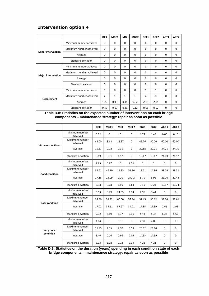
217
Intervention option 4
DCK MGE1 MGI MGE2 BGL1 BGL2 ABT1 ABT2
Minor intervention
Minimum number achieved 0 0 0 0 0 0 0 0
Maximum number achieved 0 0 0 0 0 0 0 0
Average 0 0 0 0 0 0 0 0
Standard deviation 0 0 0 0 0 0 0 0
Major intervention
Minimum number achieved 0 0 0 0 0 0 0 0
Maximum number achieved 0 0 0 0 0 0 0 0
Average 0 0 0 0 0 0 0 0
Standard deviation 0 0 0 0 0 0 0 0
Replacement
Minimum number achieved 1 0 0 0 1 1 0 0
Maximum number achieved 2 1 1 1 4 3 0 0
Average 1.29 0.03 0.11 0.02 2.18 2.14 0 0
Standard deviation 0.45 0.17 0.31 0.12 0.65 0.62 0 0
Table D.8: Statistics on the expected number of interventions on each bridge components – maintenance strategy: repair as soon as possible
DCK MGE1 MGI MGE2 BGL1 BGL2 ABT 1 ABT 2
As new condition
Minimum number achieved
0.02 0 0 0 1.77 1.48 0.06 0.16
Maximum number achieved
48.00 8.68 12.37 0 45.76 50.00 60.00 60.00
Average 15.87 0.12 0.35 0 20.58 20.71 34.71 34.10
Standard deviation 9.89 0.91 1.57 0 10.47 10.67 21.03 21.17
Good condition
Minimum number achieved
2.25 5.27 0 4.16 0 0 0 0
Maximum number achieved
34.61 46.70 15.35 51.86 13.51 14.86 59.05 59.51
Average 17.18 24.09 0.20 24.42 5.70 5.96 21.16 22.43
Standard deviation 5.98 8.03 1.50 8.84 3.10 3.24 18.57 19.34
Poor condition
Minimum number achieved
3.53 8.79 24.55 6.14 2.96 3.44 0 0
Maximum number achieved
35.60 52.82 60.00 55.84 31.45 30.62 38.34 33.61
Average 17.02 34.11 57.27 34.01 17.85 17.39 2.61 1.95
Standard deviation 7.32 8.50 5.17 9.11 5.43 5.37 6.27 5.62
Very poor condition
Minimum number achieved
4.04 0 0 0 4.37 4.05 0 0
Maximum number achieved
16.85 7.55 9.70 3.58 25.62 23.70 0 0
Average 8.40 0.16 0.66 0.05 14.33 14.39 0 0
Standard deviation 3.03 1.02 2.13 0.39 4.22 4.21 0 0
Table D.9: Statistics on the duration (years) spending in each condition state of each bridge components – maintenance strategy: repair as soon as possible


![INDEX [] · 2005-10-25 · 5 Bryant, John F, 27 Bryant, Levi Clinton, Sr, 109 Bryant, Lillie S, 101 Bryant, Linster, 101 Bryant, Litha L, 109 Bryant, Louisa M, 111 Bryant, Mary, 101](https://img.pdfslide.us/doc/110x75/5f4498e1f4a6be5e1a48d4d2/index-2005-10-25-5-bryant-john-f-27-bryant-levi-clinton-sr-109-bryant.jpg)


![[Ass.finance.group Nguyen Dieu Linh]](https://img.pdfslide.us/doc/110x75/577cd8661a28ab9e78a119cb/assfinancegroup-nguyen-dieu-linh.jpg)


![[Report] vu khanh linh](https://img.pdfslide.us/doc/110x75/55cfe635bb61eb38468b46af/report-vu-khanh-linh.jpg)