1

Abstract

This paper investigates novel LBP-guided active contour approaches to texture segmentation. The Local Binary Pattern (LBP)

operator is well suited for texture representation, combining efficiency and effectiveness for a variety of applications. In this light,

two LBP-guided active contours have been formulated, namely the scalar-LBP Active Contour (s-LAC) and the vector-LBP Active

Contour (v-LAC). These active contours combine the advantages of both the LBP texture representation and the vector-valued

Active Contour Without Edges model, and result in high quality texture segmentation. s-LAC avoids the iterative calculation of

active contour equation terms derived from textural feature vectors and enables efficient, high quality texture segmentation. v-

LAC evolves utilizing regional information encoded by means of LBP feature vectors. It involves more complex computations than

s-LAC but it can achieve higher segmentation quality. The computational cost involved in the application of v-LAC can be

reduced if it is preceded by the application of s-LAC. The experimental evaluation of the proposed approaches demonstrates

their segmentation performance on a variety of standard images of natural textures and scenes.

Keywords: Local Binary Patterns, Texture Segmentation, Active Contours.

1 Introduction

Texture segmentation methods based on active contour approaches have received considerable attention over the

past few years (Theodoridis and Koutroumbas, 2006; Paragios and Deriche, 1999; Lehmann et al, 2001; Sandberg et

al, 2002; Aujol et al, 2003; Rousson et al, 2003; Sagiv et al, 2004; Huang et al, 2004; He et al, 2004; Allili et al, 2004;

Pujol and Radeva, 2004; Lee et al, 2005), by exploiting advances in the active contour research such as contour

smoothness, noise robustness and topological adaptability. This emerging trend in the area of texture segmentation

has been reinforced by the vector formulation of recent active contour approaches (Chan et al, 2002; Sandberg and

Chan, 2005) introduced to provide a natural platform for the embedment of textural features. Such methods constitute

an essential first step in computer vision applications, which are as diverse as medical image analysis, industrial

monitoring of product quality, content-based image retrieval and remote sensing.

The main notion of the active contour approach to texture segmentation relies on the deformation of initial contours

towards the boundaries of image regions to be segmented. The deformation is realized by minimizing an energy

functional, designed so that its local minimum is reached at target boundaries. Active contour models lead to

LBP-guided Active Contours

Michalis A. Savelonas, Dimitris K. Iakovidis, and Dimitris Maroulis

Department of Informatics and Telecommunications, University of Athens, Panepistimiopolis, Illisia, GR-15784 Athens, Greece

m.savelonas, d.iakovidis, d.maroulis@di.uoa.gr

2

continuous, closed or open, curves without requiring edge-linking operations. The original active contour approach

(Kass et al, 1988) is boundary-based utilizing intensity gradients to guide contour evolution. However, in the case of

objects whose boundaries are either smooth or not necessarily defined by gradient, such methods may result in

boundary “leakage” (Chan and Vese, 2001). Moreover, the parametric formulation of the original active contour

approach does not allow for changes in the topology of the evolving contour, such as splitting or merging.

Alternative active contour approaches have been proposed to surpass the aforementioned limitations: Caselles et

al, (1997) introduced the Geodesic Active Contour (GAC) model which uses the level set method, originally proposed

in (Osher and Sethian, 1988), in order to facilitate topological adaptability. However, the GAC model inherits the

dependency on gradients of the original active contour approach and thus cannot prevent boundary “leakage” (Suri et

al, 2002). Chan and Vese, (2001) proposed the Active Contour Without Edges (ACWE) model which is a level set and

region-based active contour model, following the Mumford-Shah segmentation approach (Mumford and Shah, 1989).

The ACWE model deals with the problem of boundary “leakage” by utilizing intensity integrals calculated over the

regions inside and outside the contour. This model was later extended and then generalized by Chan et al, (2002)

and Sandberg and Chan, (2005) respectively, for vector-valued images by replacing the scalar gray-level intensities

with vectors of color channel intensities to guide contour evolution. However, the information derived from intensity

integral operations can be misleading for texture segmentation tasks as regions of different textures may have equal

average intensities. Therefore the utilization of ACWE based on image intensities can be considered unsuitable for

texture segmentation, either in its original or in its generalized form. However, its region-based formulation could be

exploited for capturing textural information, derived from features not necessarily exhibiting high gradients at object

boundaries.

Latest advances in active contour research focus on the incorporation of textural features to guide the contour

evolution. The methods that have been proposed span two categories:

1) Gabor and wavelet-based methods. Gabor-based methods involve transformation of input images into different

scales, frequencies and orientations by Gabor filtering. The associated filter-bank responses are used to generate

textural feature vectors to guide the contour evolution. In this context, Sandberg et al, (2002) proposed a method that

utilizes Gabor filter-bank responses to generate vector-valued images, successively segmented by the ACWE model

for vector-valued images (Chan et al, 2002). Paragios and Deriche, (1999) proposed a supervised texture

segmentation method, in which a Gabor filter-bank is applied to the input and to a preferable pattern image. The filter-

bank responses are represented as multi-component conditional probability density functions and a textural feature

vector encoding boundary information is generated. The maximum vector component is used to guide the GAC

model. He et al, (2004) proposed an unsupervised texture segmentation method employing Geodesic Active Regions

(Paragios, 2000) guided by the responses of a Gabor filter bank. Sagiv et al, (2004) proposed a method according to

which the input image is filtered by a Gabor filter-bank to create a feature space and extract a two-dimensional

3

Riemmannian manifold of local textural features via the Beltrami framework (Sochen et al, 1998). The textural feature

vector generated by this method is used to guide the GAC model as well as an Integrated Active Contour (IAC) model

extending both ACWE and GAC models.

The Gabor-based texture segmentation methods are credited as being state-of-the-art in texture analysis.

However, despite their theoretical elegance and their psychovisual interpretation (Sagiv et al, 2004), these methods

tend to be computationally demanding. Furthermore, Gabor filter responses are monotonic functions of gray-level

intensities. This renders Gabor-based methods sensitive to changes of the illumination conditions (Mäenpää, 2003).

Liapis et al, (2004) and Aujol et al, (2003) introduced two supervised texture segmentation methods employing the

Discrete Wavelet Frames Transform. Textural feature vectors extracted from the wavelet domain are utilized to guide

level set active contours. Wavelet features are suitable for the representation of non-stationary textures. However,

there are cases for which Gabor features result in better texture representation than wavelet features (Pichler et al,

1996; Aujol and Chan, 2006).

2) Statistical methods. Lehmann et al, (2001) proposed a supervised texture segmentation method that employs an

active contour model guided by co-occurrence matrices. This method involves the application of the active contour

model to prototype images, from which co-occurrence matrix features of target textures are extracted. Co-occurrence

matrix features are also extracted from test images, and the similarity of the prototype and the testing image features

is evaluated. The metrics, used to evaluate the similarity, weight linear combinations of the active contour model

parameters used for the segmentation of the prototype images. The active contour model parameters resulting from

these linear combinations are used for the segmentation of the test images. Pujol and Radeva, (2004) proposed a

supervised method for learning the local appearance of the texture classes based on a set of co-occurrence matrix

features. This method employs Fisher Linear Discriminant Analysis (Duda et al, 2001) to obtain an optimal reduced

feature space. It applies a Gaussian mixture model to construct a likelihood map in which each pixel is been assigned

the likelihood of representing each texture class. As a last step, they use a regularized version of the likelihood map

to guide a generalized Gradient Vector Flow active contour model (Xu and Prince, 1998). The overhead introduced in

the computation of co-occurrence matrix features as well as their moderate texture classification performance make

them unappealing for incorporation to an active contour texture segmentation framework (Randen and Husoy, 1999).

Another statistical method for texture segmentation with active contour models has been proposed by Rousson et

al, (2003). According to this method a seven-dimensional feature vector comprised of four gray-level intensity features

and three features that capture texture orientation, is built. The gray-level intensity and the textural features are

assumed to follow Parzen and Gaussian distributions, respectively. The distribution functions are embedded in a level

set active contour model inspired from (Paragios and Deriche, 1999). Huang et al, (2004) introduced a new class of

active contour models, metamorphs, which are formulated so as to integrate both shape and textural information.

Metamorphs constitute a generalization of previous parametric and level set active contour models. They capture

4

texture information using a nonparametric kernel-based approximation of the intensity probability density function

inside the contour. Allili et al, (2004) modeled the intensity distribution of each image region by a mixture of Gaussian

distributions and adopted the energy minimization approach introduced in (Kimmel, 2003). Lee et al, (2005) proposed

a framework allowing the use of image feature statistics describing intensity distribution, orientation, polarity,

anisotropy etc and applied a level set active contour model inspired by GAC and ACWE. The contour evolution

follows an equation involving an edge stopping function, which is calculated as the inverse of the determinant of a

metric tensor based on the Kullback-Leibler divergence. Awate et al, (2006) recently introduced a general active

contour framework, which facilitates the exploitation of higher-order statistics derived from various textural features.

The Local Binary Pattern (LBP) operator, introduced by Ojala et al, (1996), is defined so as to provide a condensed

encoding of local microstructures that captures textural information. It has been supported by various comparative

studies on texture analysis (Ojala et al, 1996; Paclic et al, 2002; Mäenpää and Pietikäinen, 2004) which demonstrate

that LBP texture representation can be superior to Gabor, wavelet and co-occurrence approaches, with a smaller

computational overhead. Unlike the Gabor approach, which utilizes textural features calculated from the weighted

mean of pixel values over a small neighborhood, the LBP operator considers each pixel in the neighborhood

separately, providing even more fine-grained information. The textural features estimated using the LBP operator are

invariant to any monotonic change in gray-level intensities, resulting in a robust representation of textures under

varying illumination conditions and can be made multiscale and invariant against rotation (Mäenpää, 2003).

Recent applications utilizing the LBP distributions for texture representation include object detection (Zhang et al,

2006), realtime facial expression recognition (Feng et al, 2005), and landform segmentation of light detection and

ranging imagery (Lucieer and Stein, 2005). Unsupervised texture segmentation algorithms utilizing the LBP

distributions have been mainly based on hierarchical splitting and agglomerative merging (Ojala and Pietikäinen,

1999), as well as on region-competition approaches (Qing et al, 2005). However, such methods involve iterative

calculations of histograms with potentially large numbers of bins that are computationally intensive and memory

consuming (Ojala and Pietikäinen, 1999). This fact partially reverses the advantage of small computational overhead

associated with the calculation of the LBP values. It should be noted that a texture segmentation method

encompassing the advantages of both LBP texture representation methodology and of active contours, has not yet

been proposed.

This study investigates LBP-guided active contour approaches to texture segmentation. In this context, two novel

approaches have been formulated:

1. Scalar-LBP Active Contour (s-LAC)

2. Vector-LBP Active Contour (v-LAC)

s-LAC encodes the spatial distribution of the most discriminative LBPs of an input image into gray-level intensities

producing a new image which is subsequently segmented by ACWE model. This approach avoids the iterative

5

calculation of active contour equation terms derived from textural feature vectors, and enables efficient, high quality

texture segmentation. v-LAC utilizes multidimensional feature vectors representing LBP distributions that encode the

textural properties of image regions rather than the single pixel information utilized in the case of vector-valued

ACWE. Moreover, unlike vector-valued ACWE, the similarity between the LBP distributions is quantified by means of

the log-likelihood statistic, which favors segmentations corresponding to image regions of minimum total entropy.

Although computationally demanding, v-LAC can lead to higher segmentation quality than s-LAC. In order to reduce

the computational cost involved in v-LAC segmentation the successive application of both s-LAC and v-LAC is

proposed.

The rest of this paper is organized in five sections. Sections 2 and 3 outline the ACWE model and the LBP

features, respectively. Section 4 describes the proposed s-LAC and v-LAC approaches for texture segmentation. The

results from the experimental evaluation of the proposed approaches on textures and natural scenes acquired from

standard image databases are apposed in Section 5. Finally, in Section 6 the conclusions of this study are

summarized.

2 Active Contour Without Edges

The vector-valued ACWE model as posed in (Chan et al, 2002), follows the Mumford-Shah segmentation approach

(Mumford and Shah, 1989) and has the form of a minimization problem: if we consider Ω as a bounded open subset

of 2R , with Ω∂ the boundary, we seek for the infimum of the energy functional F:

∫ ∑ −∫ ∑ +−+⋅==

−−

=+

+−+

)( 1

2

0)( 1

2

0 |),(|1

|),(|1

)(),,(Coutside

b

i

ii

iCinside

b

i

ii

i dxdycyxub

dxdycyxub

ClengthccCF λλµ (1)

where iu0 , i=1,…,b are the components that describe the original image u0, 2]1,0[:)( RsC → is a parameterized curve,

ic+ and ic− , i=1,2,…,b are unknown constants representing the average value of

iu0 inside and outside the curve, and

parameters µ, +iλ and −

iλ , i=1,…,b are weights for the regularizing term and the fitting terms, respectively. Each

component ),(0 yxu i , i=1,…,b, is defined over a single pixel (x, y). For example in (Chan et al, 2002), each ),(0 yxu i , i =

1, 2, 3 represent a component of the RGB color space at pixel (x, y). The foreground and the background regions

resulting from the segmentation of the image by the contour C, are denoted as “inside C” and “outside C”,

respectively.

The vector-valued ACWE model uses the level set method (Osher and Sethian, 1988) which provides an efficient

means for moving curves and surfaces, on a fixed regular grid, allowing for automatic topology changes, such as

merging and splitting. Following (Osher and Sethian, 1988), the curve C is represented implicitly, by the zero level set

of a Lipschitz function ,: R→Ωφ such that:

6

0),(),()(

,0),(:),()(

,0),(:),(

<∈=

>Ω∈=

=Ω∈=

yxyxCoutside

yxyxCinside

yxyxC

φ

φφ

(2)

Using the one-dimensional Dirac measure δ and the Heaviside function H, defined by:

)()( zH

dz

dz =δ ,

0

0

,0

,1)(

<

≥

=z

z

if

ifzH (3)

the level set formulation of the energy functional F is:

∫ ∑ −−∫ ∑ +−+∫ ∇⋅=Ω =

−−

Ω =+

+

Ω−+

b

i

ii

i

b

i

ii

i dxdyyxHcyxub

dxdyyxHcyxub

dxdyyxyxccF1

2

01

2

0 ))),((1(|),(|1

),((|),(|1

|),(|)),((),,( φλφλφφδµφ

(4)

By minimizing ),,( φ−+ ccF with respect to the unknown constant vectors ic+ and

ic− , the following relations are

obtained:

∫

∫=

Ω

Ω+

dxdyyxH

dxdyyxHyxu

c

i

i

)),((

)),((),(

)(0

φ

φφ (5)

∫

∫ −=

Ω

Ω−

dxdyyxH

dxdyyxHyxu

c

i

i

)),((

))),((1)(,(

)(0

φ

φφ (6)

which represent the averages of iu0 inside and outside the curve C respectively.

By keeping ic+ and

ic− fixed and by minimizing F with respect to φ , we deduce the associated Euler-Langrange

equation for φ . Parameterizing the descent direction by an artificial time 0≥t , the equation in ),,( yxtφ (with

),(),,0( 0 yxyx φφ = defining the initial contour) is:

0])(1

)(1

)()[(1

2

01

2

0 =∑ −⋅+∑ −⋅−∇∇

⋅=∂∂

=

−−

=

++b

ii

i

i

b

ii

i

i cub

cub

divt

λλφφ

µφδφ (7)

where a smooth approximation of the Heaviside function H is used, as in (Chan et al, 2002). Starting with an initial

contour, defined by 0φ , at each time step the vector averages

ic+ and ic− are updated and φ evolves according to the

partial differential equation (7). Equations (1)-(7) describe the original, scalar ACWE model (Chan and Vese, 2001)

for b=1. More details for the numerical aspects of the level set evolution can be found in (Aubert and Vese, 1997).

3 Local Binary Patterns

The LBP operator, as defined in (Ojala et al, 2002), utilizes a binary representation of local texture patterns. Let T

be such a texture pattern, defined in a local neighborhood of a gray-level texture image as the joint distribution of the

gray-levels of P (P > 1) image pixels:

),...,,( 10 −= PgggT τ (8)

7

where g is the gray-level of the central pixel of the local neighborhood and gp (p = 0,…, P-1) represents the gray-level

of P equally spaced pixels arranged on a circle of radius R (R > 0), forming a circularly symmetric neighbor set.

Assuming that the differences gp-g are not affected by changes in mean luminance g, the joint difference distribution

),...,( 10 gggg P −− −τ is invariant against gray-level shifts. Moreover, the LBP approach achieves invariance with

respect to the scaling of the gray-levels by considering H(gp-g) instead of gp-g, i.e. the joint signed difference

distribution T’:

))(),...,((' 10 ggHggHT P −−= −τ (9)

The LBP encoding is obtained by assigning a binomial factor 2p to each term H(gp-g). A unique LBPP,R value that

encodes the spatial structure of the local image texture 'T is estimated by:

∑ −=−

=

1

0, 2)(

P

p

p

pRP ggHLBP (10)

The distribution of the LBPP,R values calculated over an image region, comprises a highly discriminative feature

vector for texture segmentation, as demonstrated in various comparative studies (Ojala et al, 1996; Paclic et al, 2002;

Mäenpää and Pietikäinen, 2004). More detailed information concerning the LBP can be found in (Mäenpää and

Pietikäinen, 2004).

4 LBP-Guided Active Contours

4.1 Scalar-LBP Active Contour (s-LAC)

The underlying idea of s-LAC is to encode the spatial distribution of the most discriminative LBPP,R values of an

input image into gray-level intensities so as to produce a new image that satisfies the assumption of approximately

piecewise constant intensities. This is the basic assumption of the ACWE model, which is subsequently applied on

the new image. As this approach avoids the iterative calculation of active contour equation terms derived from textural

feature vectors, s-LAC can be more efficient than other active contour approaches.

s-LAC algorithm begins with the calculation of the LBPP,R values of all pixels of the input image I. A binary image is

assigned to each of the existent LBP values. For each i=LBPP,R(x,y), the pixel (x,y) of the binary image Bi is labeled

white, indicating the presence of the LBP value i, otherwise it is labeled black.

In the sequel, each Bi is divided into constant-sized blocks and the occurrence probability Ppvalue(i,j) of the pixel

value pvalue (white or black) in each block j of Bi is estimated. Since white pixels in Bi indicate the presence of the

LBP value i, their density may vary for regions of different texture, characterized by different LBP distributions. The

conditional entropy Hi, given an LBP value i:

∑ ∑ ⋅−=pvalue j

pvaluepvaluei jiPjiPH ),(log),( 2 (11)

can be used to evaluate the texture discrimination capability of the LBP value i. From an information-theoretic point of

8

view, eq. (11) is highly intuitive (Hermes and Buhmann, 2003). Since the conditional entropy Hi of an image with

respect to an LBP value i, measures the level of uncertainty about this value, Hi is expected to be smaller if white

pixels are mainly concentrated in some image blocks. Thus, a small value for conditional entropy Hi indicates that the

corresponding LBP value i is dominant on an image region.

The binary images Bi, i=1,2,…2P

are sorted according to their conditional entropy Hi, and the r top-ranked images

are selected. The logical OR operator is applied on the K=2r-1 non-empty combinations of the selected r binary

images. The resulting “cumulative” binary images CBk, k=1,2,…K, contain information derived from subsets of the

existent LBPs. This is in agreement with (Mäenpää, 2003), according to which an appropriately selected subset of

LBPs maintains most of the textural information associated with the set of the existent LBPs. The “cumulative” binary

image CBM with the minimum conditional entropy is selected, according to:

))(min(arg kk

HM = (12)

Equation (12) imposes that the selected “cumulative” image CBM will be comprised of regions characterized by

distinguishable white pixel densities.

In order to limit the effect of local variances in the spatial frequency of the LBPs, a Gaussian kernel WG is

convolved with CBM. This results in a smoothed image CBG of nearly homogeneous image regions, which satisfy the

assumption of ACWE model for piecewise constant intensities. Such smoothing operations have been proved to

enhance texture discrimination, as the notion of texture is undefined at the single pixel level and is always associated

with some set of pixels (Unser and Eden, 1990). The convolution with the Gaussian kernel WG ensures that the gray

level of each pixel in the smoothed image CBG depends on the distances of the LBPs, which are present in the

neighborhood of the pixel and have been associated with the texture of interest in the previous steps of the algorithm.

Furthermore, smoothing accelerates the convergence of the subsequently applied active contour (Akgul and

Kambhamettu, 2003).

In the last step of the algorithm, the ACWE model is applied to CBG. The region-based formulation of this active

contour model enables the segmentation of an image into two discrete regions, even if these regions are not explicitly

defined by high intensity gradients. In addition, the level set formulation of the ACWE model allows its adaptation to

topological changes, such as splitting or merging, in case regions of the same texture are interspersed in the image.

The steps of the proposed algorithm can be summarized as follows:

1. Calculate LBP values

For each pixel (x,y) in I Calculate LBPP,R(x,y)

2. Generate binary images Bi, i=1,2,…,2P

Initialize Bi(x,y) = 0

For each LBPP,R(x,y) do

i = LBPP,R(x,y)

9

Bi(x,y) = 1

End

3. Generate “cumulative” binary image CBM

Rank all Bi according to ξi

For each combination COMBk=Bi1, Bi2 ,… , Bil, k = 1,2,…K, l = card(COMBk) of the r top-ranked Bi do

CBk = (Bi1 OR Bi2 OR … OR Bil)

End

Find CBM using (12)

4. Smoothing and Segmentation

CBG = CBM * WG

Segment CBG using ACWE.

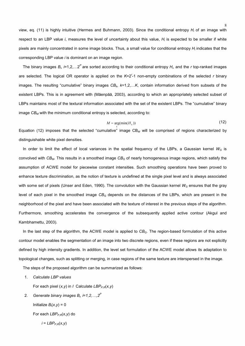
Figure 1 illustrates a schematic representation of the algorithm step by step, as applied on a composite image of

the Brodatz collection (Brodatz, 1996). Figure 2 illustrates the set COMBi of the binary images Bi1, Bi2, Bi3, Bi4

(generated at step 2) that were used to generate the cumulative image CBM at the third step of the algorithm.

10

Input image LBPP,R(x,y) ∀(x,y)

Step 1

Binary images Bi

Step 2

COMB1 COMB2 COMBK…

CB1 CB2 CBK Cumulative image

CBM

Step 3

Smoothed image

CBG

2P

Step 4

Segmented image

after ACWE

Input image LBPP,R(x,y) ∀(x,y)

Step 1

Binary images Bi

Step 2

COMB1 COMB2 COMBK…

CB1 CB2 CBK Cumulative image

CBM

Step 3

Smoothed image

CBG

2P

Step 4

Segmented image

after ACWE

Fig. 1. Schematic representation of the steps of the s-LAC algorithm and images generated at each step. The input image is Brodatz D17D55. The binary, the cumulative, and the smoothed images have been inverted for illustrational purposes.

Fig. 2. Four binary images Bi1, Bi2, Bi3, Bi4 that were used to generate the cumulative image CBM illustrated in Fig. 1. The images have been inverted for illustrational purposes.

4.2 Vector-LBP Active Contour (v-LAC)

In this section, we introduce an alternative LBP-guided active contour approach, v-LAC. As in the case of s-LAC, v-

LAC is formulated acknowledging that texture is undefined at the single pixel level and it is always associated with an

11

image region (Unser and Eden, 1996). It utilizes vectors Di(x, y), i=1,2,…,b, where each component D

i(x, y)

corresponds to the i-th bin of the LBP distribution, and b = 2P is the number of bins comprising each distribution. D

i(x,

y) encodes the textural properties of k×k-pixel image regions centered at pixel (x, y).

In order to incorporate the regional information encoded by means of LBP distributions into (1), we consider the

replacement of the vector ),(0 yxu which represents the image components at a single pixel, with Di(x, y). Moreover,

motivated by Ojala et al, (2002) in which the log-likelihood statistic is suggested as an accurate similarity measure for

LBP distributions, we consider the replacement of 2

0 |),(| ii cyxu +− and 2

0 |),(| ii cyxu −− in (1), with ))log(),(1( ii cyxD +− and

))log(),(1( ii cyxD −− respectively. These considerations lead to the derivation of a new energy functional:

∫ ∑∫ ∑=

−−

=+

+−+ −+−+⋅=′

)( 1)( 1

))log(),(1(1

))log(),(1(1

)(),,(Coutside

b

i

ii

i

Cinside

b

i

ii

i dxdycyxDb

dxdycyxDb

ClengthccCF λλµ (13)

The Euler-Langrange formulation of (13) is:

0]))log(),(1(1

))log(),(1(1

)()[(11

=−⋅+−⋅−∇∇

⋅=∂∂ ∑∑

=−

−

=+

+b

i

ii

i

b

i

ii

i cyxDb

cyxDb

divt

λλφφ

µφδφ (14)

where φ is the level set function, implicitly representing curve C.

5 Experimental Results

Experiments were performed to investigate the performance of the proposed LBP-guided active contours on

texture segmentation. The dataset used is comprised of composite texture images from the Brodatz album (Brodatz,

1996), and natural scenes from the Vistex (MIT Media Lab), Li and Wang (Li and Wang, 2003) and the Berkeley

(Martin et al, 2001) databases (examples illustrated in Fig. 3). The size of each image of the dataset used was

256×256. The active contour algorithms were implemented in Microsoft Visual C++ and executed on a 3.2 GHz Intel

Pentium IV workstation. Densely distributed small circular contours were used for the initialization of the algorithms.

As a segmentation quality measure we have considered the overlap q:

GA

GAq

∪∩

= (15)

where A is the region delineated by the algorithm and G is the ground truth region. However, this measure has been

estimated only for the segmentations of composite texture images, for which the ground truth regions are explicitly

defined.

The results are organized in three parts. The first two parts present the results obtained by s-LAC and v-LAC

approaches, whereas the third part compares the performance of the proposed LBP-guided active contours with the

performance achieved by a baseline segmentation algorithm and state of the art active contours reported in the

literature.

12

(a) (b) (c) (d)

(e) (f) (g) (h)

(i) (j) (k) (l)

(m) (n) (o) (p)

(q) (r) (s) (t)

Fig. 3. Test images from the dataset used in the experiments: (a) Brodatz D4D84, (b) Brodatz D8D84 (c) Brodatz D17D55, (d) Brodatz D9D77, (e) Brodatz D6D17, (f) Brodatz D3D5, (g) Brodatz D56D56 (re-scaled), (h) Brodatz D38D106, (i) Brodatz D17D24, (j) Brodatz D79D5, (k) Vistex Fabric2Fabric1, (l) Vistex Fabric10Fabric13, (m) Vistex Fabric5Fabric7, (n) Vistex Food0Food5 (o) Vistex Fabric09Brick05 (p) Vistex ValleyWater1, (q) Vistex GroundWaterCity1, (r) Wang 804, (s) Berkeley 28096, and (t) Vistex GrassPlantSky6.

13

5.1 s-LAC segmentation results

The LBP operator considered in the experiments with s-LAC was LBP8,1. The parameters involved were determined

by performing preliminary segmentation experiments on a randomly selected subset of the available dataset

(comprised of the images (a)-(d) of Fig. 3). The block size was set at 16×16 pixels, as this provided the highest

average overlap on this subset. Moreover, a total of r=5 top-ranked binary images in the third step of the s-LAC

algorithm was found to be sufficient for the performed segmentation tasks, as for r>5 a marginal improvement of the

segmentation quality was observed.

A rough grid search of the parameter space of the active contour was performed on the subset of images selected

for parameter tuning. Subsequent grid searches were performed for fine tuning within smaller ranges around the

highest average parameter values obtained from the rough parameter search. The highest average overlap was

obtained for 5== −+ λλ and 225601.0 ⋅=µ . The values of the parameters +λ and −λ were considered to be equal to

each other, and the values of µ where considered proportional to the image size, in accordance with (Chan and Vese,

2001). It was observed that a variation of approximately 10% of +λ and −λ , and of approximately 30% of µ around

the values used results in overlap values that differ no more than 1.0%. This indicates that slight perturbations of +λ

and −λ have a greater impact on the obtained overlaps than slight perturbations of µ .

Figure 4 illustrates example segmentation results obtained by the application of s-LAC on the images of Fig.3. The

overlaps measured are presented in Table 1. Their average overlap is estimated to be 95.2±2.9%. The results show

that s-LAC managed to segment all the composite Brodatz images accurately. It is worth noting that the segmentation

is quite satisfying even for the Brodatz images D3D5, D38D106 and D79D5 illustrated in Fig. 4f, 4h and 4h

respectively, which contain non-stationary textures.

Table 1

Overlaps obtained by the s-LAC algorithm for the segmentation of the images illustrated in Fig. 3. .

Image Overlap (%)

Image Overlap (%)

Image Overlap (%)

a 99.0 f 87.5 k 96.7

b 99.2 g 98.5 l 97.1

c 96.1 h 93.1 m 94.3

d 93.9 i 95.6 n 92.8

e 95.4 j 94.7 o 94.2

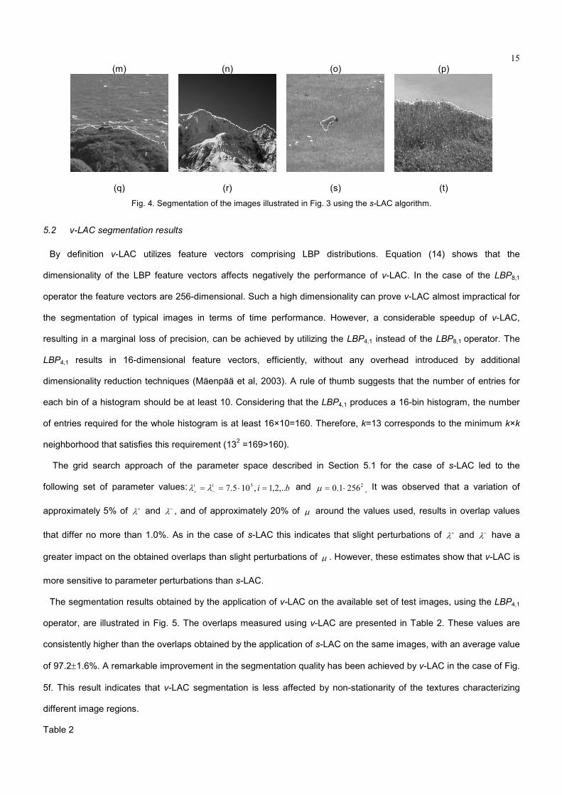
The segmentations obtained by the application of s-LAC on the natural scenes illustrated in Figs. 4o-4t,

14

demonstrate the robustness of s-LAC to illumination changes, which is mainly attributed to the LBP texture

representation. It can be observed that the textures of natural scenes are generally less uniform than the

homogeneous textures of the test mosaics. In addition, due to the infinite scale of texture differences present in such

images, choosing the right scale is a very subjective matter. For these reasons, there is often no ‘correct’

segmentation for a natural scene (Ojala and Pietikäinen, 1999). The bird illustrated in Fig. 4s has been successfully

localized by s-LAC, although it occupies a rather small portion of the image. However, the roughly defined boundaries

indicate that the statistical sample of LBPs within the bird’s region may not be sufficient to differentiate its textural

content from the surrounding background.

The convergence times of s-LAC observed for the available images, range between 3 and 4 seconds depending on

the complexity of the target boundaries.

(a) (b) (c) (d)

(e) (f) (g) (h)

(i) (j) (k) (l)

15

(m) (n) (o) (p)

(q) (r) (s) (t)

Fig. 4. Segmentation of the images illustrated in Fig. 3 using the s-LAC algorithm.

5.2 v-LAC segmentation results

By definition v-LAC utilizes feature vectors comprising LBP distributions. Equation (14) shows that the

dimensionality of the LBP feature vectors affects negatively the performance of v-LAC. In the case of the LBP8,1

operator the feature vectors are 256-dimensional. Such a high dimensionality can prove v-LAC almost impractical for

the segmentation of typical images in terms of time performance. However, a considerable speedup of v-LAC,

resulting in a marginal loss of precision, can be achieved by utilizing the LBP4,1 instead of the LBP8,1 operator. The

LBP4,1 results in 16-dimensional feature vectors, efficiently, without any overhead introduced by additional

dimensionality reduction techniques (Mäenpää et al, 2003). A rule of thumb suggests that the number of entries for

each bin of a histogram should be at least 10. Considering that the LBP4,1 produces a 16-bin histogram, the number

of entries required for the whole histogram is at least 16×10=160. Therefore, k=13 corresponds to the minimum k×k

neighborhood that satisfies this requirement (132 =169>160).

The grid search approach of the parameter space described in Section 5.1 for the case of s-LAC led to the

following set of parameter values: biii ,..2,1,105.7 5 =⋅== −+ λλ and 22561.0 ⋅=µ . It was observed that a variation of

approximately 5% of +λ and −λ , and of approximately 20% of µ around the values used, results in overlap values

that differ no more than 1.0%. As in the case of s-LAC this indicates that slight perturbations of +λ and −λ have a

greater impact on the obtained overlaps than slight perturbations of µ . However, these estimates show that v-LAC is

more sensitive to parameter perturbations than s-LAC.

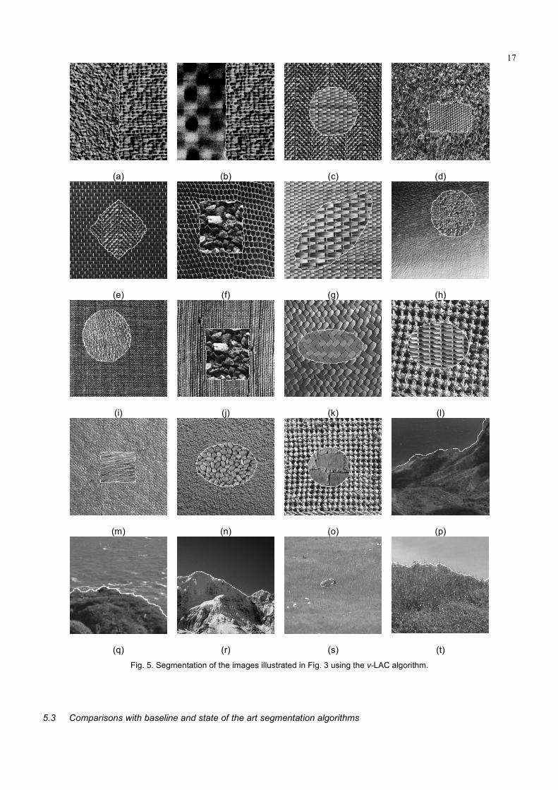
The segmentation results obtained by the application of v-LAC on the available set of test images, using the LBP4,1

operator, are illustrated in Fig. 5. The overlaps measured using v-LAC are presented in Table 2. These values are

consistently higher than the overlaps obtained by the application of s-LAC on the same images, with an average value

of 97.2±1.6%. A remarkable improvement in the segmentation quality has been achieved by v-LAC in the case of Fig.

5f. This result indicates that v-LAC segmentation is less affected by non-stationarity of the textures characterizing

different image regions.

Table 2

16

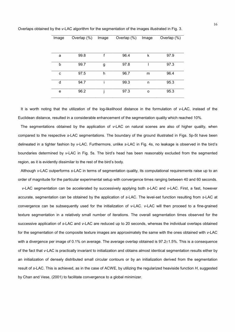
Overlaps obtained by the v-LAC algorithm for the segmentation of the images illustrated in Fig. 3.

Image Overlap (%)

Image Overlap (%)

Image Overlap (%)

a 99.8 f 96.4 k 97.9

b 99.7 g 97.8 l 97.3

c 97.5 h 96.7 m 96.4

d 94.7 i 99.3 n 95.3

e 96.2 j 97.3 o 95.3

It is worth noting that the utilization of the log-likelihood distance in the formulation of v-LAC, instead of the

Euclidean distance, resulted in a considerable enhancement of the segmentation quality which reached 10%.

The segmentations obtained by the application of v-LAC on natural scenes are also of higher quality, when

compared to the respective s-LAC segmentations. The boundary of the ground illustrated in Figs. 5p-5t have been

delineated in a tighter fashion by v-LAC. Furthermore, unlike s-LAC in Fig. 4s, no leakage is observed in the bird’s

boundaries determined by v-LAC in Fig. 5s. The bird’s head has been reasonably excluded from the segmented

region, as it is evidently dissimilar to the rest of the bird’s body.

Although v-LAC outperforms s-LAC in terms of segmentation quality, its computational requirements raise up to an

order of magnitude for the particular experimental setup with convergence times ranging between 40 and 60 seconds.

v-LAC segmentation can be accelerated by successively applying both s-LAC and v-LAC. First, a fast, however

accurate, segmentation can be obtained by the application of s-LAC. The level-set function resulting from s-LAC at

convergence can be subsequently used for the initialization of v-LAC. v-LAC will then proceed to a fine-grained

texture segmentation in a relatively small number of iterations. The overall segmentation times observed for the

successive application of s-LAC and v-LAC are reduced up to 20 seconds, whereas the individual overlaps obtained

for the segmentation of the composite texture images are approximately the same with the ones obtained with v-LAC

with a divergence per image of 0.1% on average. The average overlap obtained is 97.2±1.5%. This is a consequence

of the fact that v-LAC is practically invariant to initialization and obtains almost identical segmentation results either by

an initialization of densely distributed small circular contours or by an initialization derived from the segmentation

result of s-LAC. This is achieved, as in the case of ACWE, by utilizing the regularized heaviside function H, suggested

by Chan and Vese, (2001) to facilitate convergence to a global minimizer.

17

(a) (b) (c) (d)

(e) (f) (g) (h)

(i) (j) (k) (l)

(m) (n) (o) (p)

(q) (r) (s) (t)

Fig. 5. Segmentation of the images illustrated in Fig. 3 using the v-LAC algorithm.

5.3 Comparisons with baseline and state of the art segmentation algorithms

18

As a baseline to compare the segmentation quality obtained by s-LAC and v-LAC we have considered the JSEG

image segmentation algorithm (Deng and Manjunath, 2001). JSEG was applied on each composite image of the

available dataset, for multiple combinations of its parameters (scales 1-4; quantization threshold 0-600; and region

merging threshold 0.0-1.0). The highest overlaps achieved for each composite image are presented in Table 3 and

can be considered as a means to evaluate the difficulty to segment these images. It can be observed that both s-LAC

and v-LAC obtain higher overlaps than JSEG. Moreover, JSEG obtains lower overlaps in images which contain non-

stationary textures, as it is the case with Fig. 3f, 3h and 3j, indicating that these images pose the most challenging

segmentation tasks.

Table 3

Overlaps obtained by a baseline algorithm (JSEG) for the segmentation of the images illustrated in Fig. 3.

Image Overlap (%)

Image Overlap (%)

Image Overlap (%)

a 72.3 f 58.1 k 62.8

b 68.7 g 62.3 l 63.2

c 94.2 h 59.6 m 64.0

d 78.9 i 91.4 n 64.5

e 88.7 j 56.8 o 92.1

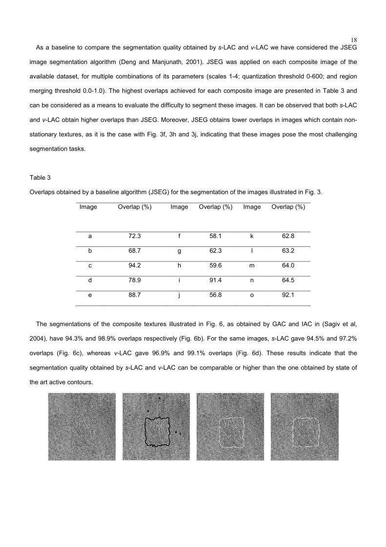
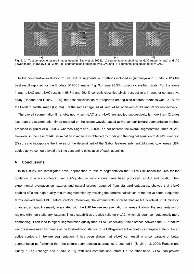
The segmentations of the composite textures illustrated in Fig. 6, as obtained by GAC and IAC in (Sagiv et al,

2004), have 94.3% and 98.9% overlaps respectively (Fig. 6b). For the same images, s-LAC gave 94.5% and 97.2%

overlaps (Fig. 6c), whereas v-LAC gave 96.9% and 99.1% overlaps (Fig. 6d). These results indicate that the

segmentation quality obtained by s-LAC and v-LAC can be comparable or higher than the one obtained by state of

the art active contours.

19

(a) (b) (c) (d)

Fig. 6. (a) Test composite texture images used in (Sagiv et al, 2004), (b) segmentations obtained by GAC (upper image) and IAC (lower image) in (Sagiv et al, 2004), (c) segmentations obtained by s-LAC and (d) segmentations obtained by v-LAC.

In the comparative evaluation of five texture segmentation methods included in (Acharyya and Kundu, 2001) the

best result reported for the Brodatz D17D55 image (Fig. 3c), was 98.3% correctly classified pixels. For the same

image, s-LAC and v-LAC results in 98.7% and 99.4% correctly classified pixels, respectively. In another comparative

study (Randen and Husoy, 1999), the best classification rate reported among nine different methods was 98.1% for

the Brodatz D4D84 image (Fig. 3a). For the same image, s-LAC and v-LAC achieved 99.0% and 99.8% respectively.

The overall segmentation time, obtained when s-LAC and v-LAC are applied successively, is more than 12 times

less than the segmentation times reported on the recent wavelet-based active contour texture segmentation method

proposed in (Aujol et al, 2003), whereas Sagiv et al, (2004) do not address the overall segmentation times of IAC.

However, in the case of IAC, illumination invariance is obtained by modifying the original equation of ACWE evolution

(7) so as to incorporate the inverse of the determinant of the Gabor features submanifold’s metric, whereas LBP-

guided active contours avoid the time consuming calculation of such quantities.

6 Conclusions

In this study, we investigated novel approaches to texture segmentation that utilize LBP-based features for the

guidance of active contours. Two LBP-guided active contours have been proposed: s-LAC and v-LAC. Their

experimental evaluation on textures and natural scenes, acquired from standard databases, showed that s-LAC

enables efficient, high quality texture segmentation by avoiding the iterative calculation of the active contour equation

terms derived from LBP feature vectors. Moreover, the experiments showed that s-LAC is robust to illumination

changes, a capability mainly associated with the LBP texture representation, whereas it allows the segmentation of

regions with non-stationary textures. These capabilities are also valid for v-LAC, which although computationally more

demanding, it can lead to higher segmentation quality than s-LAC, especially if the distance between the LBP feature

vectors is measured by means of the log-likelihood statistic. The LBP-guided active contours compete state of the art

active contours in texture segmentation. It has been shown that s-LAC can result in a comparable or better

segmentation performance than the texture segmentation approaches presented in (Sagiv et al, 2004; Randen and

Husoy, 1999; Acharyya and Kundu, 2001), with less computational effort. On the other hand, v-LAC can provide

20

segmentations of higher quality at the cost of time performance. The iterations of the v-LAC algorithm can be reduced

by the successive application of s-LAC and v-LAC, thus requiring less computational effort than the active contours in

(Aujol et al, 2003; Sagiv et al, 2004) to perform the segmentation task.

In the experimental evaluation of the proposed LBP-guided active contours, we considered LBPs of a single pixel

radius, favoring microtexture segmentation and computational efficiency. However, in case of macrotextures, larger

LBP radii could be straightforwardly used instead. Depending on the application, further optimizations of the proposed

LBP-guided active contours could also include the utilization of the rotation invariant LBP operator (Ojala et al, 2002),

as well as of the multiphase active contour formulation (Vese and Chan, 2002) for the segmentation of multiple

textures.

Future perspectives of this work include the formulation of LBP-guided active contours for bimodal segmentation of

textures with stationary global minimum (Lee and Seo, 2006), and applications on various domains, including medical

and satellite images.

Acknowledgment

This work was supported by the Greek General Secretariat of Research and Technology and the European Social Fund, through the PENED 2003 program (grant no. 03-ED-662).

References

Acharyya, M., Kundu, M.K., 2001. An Adaptive Approach to Unsupervised Texture Segmentation Using M-Band Wavelet Transform. Sig. Proc. 81,

1337-1356.

Akgul, Y.S., Kambhamettu, C., 2003. A Coarse-to-Fine Deformable Contour Optimization Framework. IEEE Trans. on Patt. Anal. Mach. Intell. 25

(2), 174-186.

Allili, M.S., Ziou, D., Bentabet, L., 2004. A Robust Level Set Approach for Image Segmentation and Statistical Modeling. In: Proc. Adv. Conc. Intell.

Vis. Syst. (ACIVS), pp. 243-251.

Aubert, G., Vese, L., 1997. A Variational Method in Image Recovery. SIAM J. Num. Anal. 34 (5), 1948-1979.

Aujol, J.F., Aubert, G., Blanc-Feraud, L., 2003. Wavelet-Based Level Set Evolution for Classification of Textured Images. IEEE Trans. Im. Proc. 12

(12), 1634-1641.

Aujol, J.F., Chan, T.F., 2006. Combining Geometrical and Textured Information to Perform Image Classification. J. Vis. Comm. Im. Repr. 17 (5)

1004-1023.

Awate S.P., Tasdizen T., Whitaker R.T., 2006. Unsupervised Texture Segmentation with Nonparametric Neighborhood Statistics. In: Proc. Eur.

Conf. Comp. Vis. (ECCV), 494-507.

Brodatz, P., 1996. Textures: A Photographic Album for Artists and Designers, New York, NY, Dover.

Caselles, V., Kimmel R., Sapiro, G., 1997. Geodesic Active Contours. Int. J. Comp. Vis. 22, 61-79.

Chan, T., Sandberg, B., Vese, L., 2002. Active Contours Without Edges for Vector-Valued Images. J. Vis. Comm. Im. Repr. 11, 130-141.

Chan, T.F., Vese, L.A., 2001. Active Contours Without Edges. IEEE Trans. Im. Proc. 7, 266-277.

Deng, Y., Manjunath, B.S., 2001. Unsupervised Segmentation of Color-Texture Regions in Images and Video. IEEE Trans. on Patt. Anal. Mach.

Intell. 23 (8), 800-810.

21 Duda, R.O., Hart, P.E., Stork, D.G., 2001. Pattern Classification. 2nd edition, Willey.

Feng, X., Pietikäinen, M., Hadid, A., Xie, H., 2005. A Novel Real Time System for Facial Expression Recognition. In: Proc. Aff. Comput. Intell. Inter.,

Lect. Not. Comp. Sc. 3784, pp. 248-256.

He, Y., Luo, Y., Hu, D., 2004. Unsupervised Texture Segmentation via Applying Geodesic Active Regions to Gaborian Feature Space. IEEE Trans.

Eng., Comp. Tech., 272-275.

Hermes, L., Buhmann, J.M., 2003. A Minimum Entropy Approach to Adaptive Image Polygonization. IEEE Trans. Im. Proc. 12 (10), 1243-1258.

Huang, X., Metaxas, D., Chen, T., 2004. Metamorphs: Deformable Shape and Texture Models. In: Proc IEEE Int. Conf. Comp. Vis. Patt. Rec.

(ICVPR), 1496-1503.

Kass, M., Witkin, A., Terzopoulos, D., 1988. Snakes: Active Contour Models. Int. J. Comp. Vis. 1, 321-331.

Kimmel, R., 2003. Geometric Level Set Methods in Imaging, Vision and Graphics. Springer-Verlag.

Lee, S.H., Seo, J.K., 2006. Level Set-Based Bimodal Segmentation with Stationary Global Minimum. IEEE Trans. Im. Proc. 15(9), 2843-2852.

Lee, S.M., Abott, A.L., Clark, N.A., Araman, P.A., 2005. Active Contours on Statistical Manifolds and Texture Segmentation. In: Proc. IEEE Int.

Conf. Im. Proc. (ICIP) 3, 828-831.

Lehmann, T., Bredno, J., Spitzer, K., 2001. Texture-Adaptive Active Contour Models. In: Proc. Int. Conf. Adv Patt. Rec., Vol. 2013, 387-396.

Li, J., Wang, J.Z., 2003. Automatic linguistic indexing of pictures by a statistical modeling approach. IEEE Trans. Patt. Anal. Mach. Intell. 25 (9),

1075-1088.

Liapis, S., Sifakis, E., Tziritas, G., 2004. Colour and Texture Segmentation Using Wavelet Frame Analysis, Deterministic Relaxation, and Fast

Marching Algorithms. J. Vis. Comm. Im. Repr. 15, 1-26.

Lucieer, A., Stein, A., 2005. Texture-Based Landform Segmentation of LiDAR Imagery. Int. J. Appl. Earth Obs. Geoinf. 6, 261-270.

Mäenpää, T., 2003. The Local Binary Pattern Approach to Texture Analysis- Extensions and Applications,” PhD dissertation, Dept. of Elec. Inf.

Eng., Oulou University, Finland.

Mäenpää, T., Pietikäinen, M., 2004. Classification with color and texture: Jointly or separately? Patt. Rec. 37 (8), 1629-1640.

Mäenpää, T., Viertola J., Pietikäinen, M., 2003. Optimising Colour and Texture Features for Real-Time Visual Inspection. Patt. Anal. Appl. 6 (3),

169-175.

Martin, D., Fowlkes, C., Malik, J., 2001. A database of human segmented natural images and its application to evaluating segmentation algorithms

and measuring ecological statistics. In: Proc. Int. Conf. Comp. Vis. (ICCV), 416-425.

Mumford, D., Shah, J., 1989. Optimal Approximation by Piecewise Smooth Functions and Associated Variational Problems. Comm. Pur. Appl.

Math. 42, 577-685.

Ojala, T., Pietikäinen, M., 1999. Unsupervised Texture Segmentation Using Feature Distributions. Pat. Rec. 32 (3), 477-486.

Ojala, T., Pietikäinen, M., Harwood, D., 1996. A Comparative Study of Texture Measures with Classification based on Feature Distributions,” Pat.

Rec. 29, 51-59.

Ojala, T., Pietikäinen, M., Mäenpää, T., 2002. Multiresolution Gray-Scale and Rotation Invariant Texture Classification with Local Binary Patterns.

IEEE Trans. Patt. Anal. Mach. Intell. 24 (7), 971-987.

Osher S., Sethian, J., 1988. Fronts Propagating with Curvature- Dependent Speed: Algorithms Based on the Hamilton-Jacobi Formulations. J.

Comp. Phys. 79, 12-49.

Paclic, P., Duin, R., Kempen, G.V., Kohlus, R., 2002. Supervised Segmentation of Textures in Backscatter Images. In: Proc. IEEE Int. Conf. on

Patt. Rec. (ICPR) 2, pp. 490-493.

Paragios, N., 2000. Geodesic Active Regions and Level Set Methods: Contributions and Applications in Artificial Vision. PhD dissertation, Sch. of

Comp. Eng., Univ. of Nice, Sophia, Antipolis, France.

22 Paragios, N., Deriche, R., 1999. Geodesic Active Contours for Supervised Texture Segmentation. In: Proc. IEEE Int. Conf. on Com. Vis. Patt. Rec.,

pp. 2422-2427.

Pichler, O., Teuner, A., Hosticka, B.J., 1996. A Comparison of Texture Feature Extraction Using Adaptive Gabor Filtering, Pyramidal and

Structured Wavelet Transforms. Patt. Rec. 29 (5), 733-742.

Pujol, O., Radeva, P., 2004. Texture Segmentation by Statistic Deformable Models. Int. J. Im. Graph. 4 (3) 433-452.

Qing, X., 2005. Texture Segmentation Using LBP Embedded Region Competition. El. Lett. Comp. Vis. Im. Anal. 5 (1), 41-47.

Randen, T., Husøy, J.H., 1999. Filtering for Texture Classification: A Comparative Study. IEEE Trans. Patt. Anal. Mach. Intell. 21 (4), 291-310.

Rousson, M., Brox, T., Deriche, R., 2003. Active Unsupervised Texture Segmentation on a Diffusion Based Feature Space. In: Proc. IEEE Int.

Conf. Comp. Vis. Patt. Rec., Madison, Wisconsin, USA.

Sagiv, C., Sochen, N.A., Zeevi, Y., 2004. Integrated Active Contours for Texture Segmentation. IEEE Trans. Im. Proc. 1 (1), 1-19.

Sandberg, B., Chan, T.F., 2005. A Logic Framework for Active Contours on Multi-Channel Images. J. Vis. Comm. Im. Repr. 16, 333-358.

Sandberg, B., Chan, T., Vese, L., 2002. A Level-Set and Gabor-based Active Contour Algorithm for Segmenting Textured Images. In: Technical

Report 39, Math. Dept. UCLA, Los Angeles, USA.

Sochen, N., Kimmel, R., Malladi, R., 1998. A General Framework for Low Level Vision. IEEE Trans. Im. Proc. 7, 310-318.

Suri, J.S., Liu, K., Laxminarayan, S.N., Zeng, X., Reden, L, 2002. Shape Recovery Algorithms Using Level Sets in 2-D/3-D Medical Imagery: A

State-of-the-Art Review. ΙΕΕΕ Trans. Inf. Tech. Biom. 6 (1), 8-28.

Theodoridis, S., Koutroumbas, K., 2006. Pattern Recognition, 3rd edition, Academic Press.

Unser M., Eden, M., 1990. Nonlinear Operators for Improving Texture Segmentation Based on Features Extracted by Spatial Filtering. IEEE Trans.

Syst., Man .Cyber. 20 (4), 804-815.

Vese, L.A., Chan, T.F., 2002. A Multiphase Level Set Framework for Image Segmentation Using the Mumford and Shah Model. Int. J. Comp. Vis.

50 (3), 271-293.

Vision Texture Database, MIT Media Lab, www-white.media.mit.edu/vismod/imagery/ VisionTexture/vistex.html.

Xu, C., Prince, J.L., 1998. Generalized Gradient Vector Flow External Forces for Active Contours. Sig. Proc. 71, 131-139.

Zhang, H., Gao, W., Chen, X., Zhao, D., 2006.Object Detection Using Spatial Histogram Features. Im. Vis. Comp. 24, 327-341.