Embed Size (px)
Citation preview

eScholarship provides open access, scholarly publishingservices to the University of California and delivers a dynamicresearch platform to scholars worldwide.
Lawrence Berkeley National Laboratory
Title:Massively-parallel electrical-conductivity imaging of hydrocarbons using the Blue Gene/Lsupercomputer
Author:Commer, M.Newman, G.A.Carazzone, J.J.Dickens, T.A.Green, K.E.Wahrmund, L.A.Willen, D.E.Shiu, J.
Publication Date:06-24-2008
Publication Info:Lawrence Berkeley National Laboratory
Permalink:http://escholarship.org/uc/item/3mp5q7pp
Abstract:Large-scale controlled source electromagnetic (CSEM) three-dimensional (3D) geophysicalimaging is now receiving considerable attention for electrical conductivity mapping of potentialoffshore oil and gas reservoirs. To cope with the typically large computational requirements ofthe 3D CSEM imaging problem, our strategies exploit computational parallelism and optimizedfinite-difference meshing. We report on an imaging experiment, utilizing 32,768 tasks/processorson the IBM Watson Research Blue Gene/L (BG/L) supercomputer. Over a 24-hour period, wewere able to image a large scale marine CSEM field data set that previously required over fourmonths of computing time on distributed clusters utilizing 1024 tasks on an Infiniband fabric. Thetotal initial data misfit could be decreased by 67 percent within 72 completed inversion iterations,indicating an electrically resistive region in the southern survey area below a depth of 1500 mbelow the seafloor. The major part of the residual misfit stems from transmitter parallel receivercomponents that have an offset from the transmitter sail line (broadside configuration). Modelingconfirms that improved broadside data fits can be achieved by considering anisotropic electricalconductivities. While delivering a satisfactory gross scale image for the depths of interest, theexperiment provides important evidence for the necessity of discriminating between horizontaland vertical conductivities for maximally consistent 3D CSEM inversions.

MASSIVELY-PARALLEL ELECTRICAL-CONDUCTIVITY IMAGING 1
OF HYDROCARBONS USING THE BLUE GENE/L SUPERCOMPUTER 2
3
M. Commer & G. A. Newman 4
Lawrence Berkeley National Laboratory 5
6
J. J. Carazzone, T. A. Dickens, K. E. Green, L. A. Wahrmund & D. E. Willen 7
ExxonMobil Upstream Research Company 8
9
J. Shiu 10
Deep Computing IBM Corporation 11
12
ABSTRACT 13
Large-scale controlled source electromagnetic (CSEM) three-dimensional (3D) 14
geophysical imaging is now receiving considerable attention for electrical conductivity 15
mapping of potential offshore oil and gas reservoirs. To cope with the typically large 16
computational requirements of the 3D CSEM imaging problem, our strategies exploit 17
computational parallelism and optimized finite-difference meshing. We report on an 18
imaging experiment, utilizing 32,768 tasks/processors on the IBM Watson Research Blue 19
Gene/L (BG/L) supercomputer. Over a 24-hour period, we were able to image a large-20
scale marine CSEM field data set that previously required over four months of computing 21
time on distributed clusters utilizing 1024 tasks on an Infiniband fabric. The total initial 22

data misfit could be decreased by 67 % within 72 completed inversion iterations, 23
indicating an electrically resistive region in the southern survey area below a depth of 24
1500 m below the seafloor. The major part of the residual misfit stems from transmitter-25
parallel receiver components that have an offset from the transmitter sail line (broadside 26
configuration). Modeling confirms that improved broadside data fits can be achieved by 27
considering anisotropic electrical conductivities. While delivering a satisfactory gross-28
scale image for the depths of interest, the experiment provides important evidence for the 29
necessity of discriminating between horizontal and vertical conductivities for maximally 30
consistent 3D CSEM inversions. 31
32
INTRODUCTION 33
Seismic methods have a long and established history in hydrocarbon, i.e. oil and gas, 34
exploration, and are proven very effective in mapping geologic reservoir formations. 35
However, they are not good at discriminating the different types of reservoir fluids 36
contained in the rock pore space, such as brines, water, oil and gas. This has encouraged 37
the development of new geophysical technologies that can be combined with established 38
seismic methods to directly image fluids. One technique that has recently emerged, with 39
considerable potential, utilizes low frequency electromagnetic (EM) energy to map 40
variations in the subsurface electrical conductivity, σ ([σ]=S/m), or its reciprocal 41
([1/σ]=Ωm), usually called resistivity, of offshore oil and gas prospects [1, 2, 3, 4 and 5]. 42
Resistivity is a more meaningful quantity for imaging hydrocarbons. An increase, 43
compared to the surrounding geological strata, may directly indicate potential reservoirs. 44

EM field measurements have been shown to be highly sensitive to changes in the pore 45
fluid types and the location of hydrocarbons, given a sufficient resistivity contrast to fluids 46
like brine or water. 47
With the marine controlled-source electromagnetic (CSEM) measurement technique, a 48
deep-towed electric-dipole transmitter is used to excite a low-frequency (~0.1 to 10 Hz) 49
electromagnetic signal that is measured on the seafloor by electric and magnetic field 50
detectors, where the largest transmitter-detector offsets can exceed 15 km. To cover larger 51
depth ranges, multiple transmitter frequencies are usually employed in a survey. Similar to 52
acoustic wave propagation, the attenuation rate with exploration depth increases with the 53
frequency. Current technologies require low frequency EM signals (< 1 Hz) to interrogate 54
down to reservoir depths as large as 4 km. 55
Exploration with the CSEM technology in the search for hydrocarbons now extends to 56
highly complex and subtle offshore geological environments. The geometries of the 57
reservoirs are inherently 3D and exceedingly difficult to map without recourse to 3D EM 58
imaging experiments, requiring fine model parameterizations, spatially exhaustive survey 59
coverage and multi-component data. The 3D imaging problem, in this paper also referred 60
to as inversion problem, usually has large computational demands, owing to the expensive 61
solution of the forward modeling problem, that is the EM field simulation on a given 3D 62
finite-difference (FD) grid. Moreover, large data volumes require many forward solutions 63
in an iterative inversion scheme. Therefore, we have developed an imaging algorithm that 64
utilizes two levels of parallelization, one over the modeling/imaging volume, and the other 65
over the data volume. The algorithm is designed for arbitrarily large data sets, allowing for 66
an arbitrarily large number of parallel tasks, while the computationally idle message 67
passing is minimized. We have further incorporated an optimal meshing scheme that 68
allows us to separate the imaging/modeling mesh from the simulation mesh. This provides 69
for significant acceleration of the 3D EM field simulation, directly impacting the time to 70
solution for the 3D imaging process. 71
Here, we report an imaging experiment, utilizing 32,768 tasks/processors on the IBM 72
Watson Research BG/L supercomputer. The experiment is a novelty both in terms of 73
computational resources utilized and amount of data inverted. Its main purpose is a 74
feasibility study for the effectiveness of the employed algorithm. Further, the results 75
obtained will improve both important base knowledge for the design of upcoming large-76
scale CSEM surveys and the automated imaging method for data interpretation. 77
78
79
PROBLEM FORMULATION 80
We formulate the inverse problem by finding a model m with m piecewise constant 81
electrical conductivity parameters that describe the earth model reproducing a given data 82
set. Specifically, the inversion algorithm minimizes the error functional, 83
φ = ½ D(dp - dobs)T*D(dp - dobs) + ½ λ WmTWm, (1) 84
where T* denotes the Hermitian conjugate operator. In the above expression, the predicted 85
(from a starting model) and observed data vectors are denoted by dp and d
obs, respectively, 86
where each has n complex values. These vectors consist of electric or magnetic field 87

values specified at the measurement points, where the predicted data are determined 88
through solution of the time harmonic 3D Maxwell equations in the diffusive 89
approximation. We have also introduced a diagonal weighting matrix, Dnxn, into the error 90
functional to compensate for noisy measurements. To stabilize the minimization of (1) and 91
to reduce model curvature in three dimensions, we introduce a matrix Wmxm based upon a 92
FD approximation to the Laplacian (∇2) operator applied in Cartesian coordinates. The 93
parameter λ attempts to balance the data error and the model smoothness constraint. 94
95
The Forward Problem 96
Within an inversion framework, the forward problem is solved multiple times to simulate 97
the EM field, denoted by the vector E, and thus the data dp for a given model m. EM wave 98
propagation is controlled by the vector Helmholtz equation, 99
Jii 00 ωµσωµ −=Ε+Ε×∇×∇ (2)
where source vector, free-space magnetic permeability, and angular frequency are denoted 100
by J, µ0, and ω, respectively (see [6] for specific details). Our solution method is based 101
upon the consideration that the number of model parameters required to simulate realistic 102
3D distributions of the electrical conductivity σ can typically exceed 107. FD modeling 103
schemes are ideally suited for this task and can be parallelized to handle large-scale 104
problems that cannot be easily treated otherwise [6]. After approximating equation (2) on a 105
staggered grid at a specific angular frequency, using finite differencing and eliminating the 106
magnetic field, we obtain a linear system for the electric field, 107

108
KE=S (3)
109
where K is a sparse complex symmetric matrix with 13 non-zero entries per row [6]. The 110
diagonal entries of K depend explicitly on the conductivity parameters that we seek to 111
estimate through the inversion process. Since the electric field, E, also depends upon the 112
conductivity, implicitly, this gives rise to the nonlinearity of the inverse problem. The 113
fields are sourced with a grounded wire or loop embedded within the modeling domain, 114
described by the discrete source vector, S, and includes Dirichlet boundary conditions 115
imposed upon the problem. To help avoid excessive meshing near the source, we favor a 116
scattered-field formulation to the forward modeling problem. In this instance, E is 117
replaced with Es in equation (3). The source term, for a given transmitter, will now depend 118
upon the difference between the 3D conductivity model and a simple background model, 119
weighted by the background electric field Eb, where E=Eb+ Es. Simple background 120
models with one-dimensional (1D) conductivity distributions, i.e. σ changes only with 121
depth, are used because fast semi-analytical solutions for Eb are available. Given the 122
solution of the electric field in equation (3), the magnetic field can be easily determined 123
from a numerical implementation of Faraday’s law. An efficient solution process is 124
paramount. We solve equation (3) to a predetermined error level using iterative Krylov 125
subspace methods, using either a biconjugate gradient (BICG) or quasi-minimum residual 126
(QMR) scheme with preconditioning [6]. 127
128

Minimization Procedure 129
In large-scale nonlinear inverse problems, as considered here, we minimize (1) using 130
gradient-based optimization techniques because of their minimal storage and 131
computational requirements. We characterize these methods as gradient-based techniques 132
because they employ only first derivative information of the error functional in the 133
minimization process, specifically -∇∇∇∇φ. Gradient-based methods include steepest decent, 134
nonlinear conjugate gradient and limited memory quasi-Newton schemes, where the latter 135
usually provide the best inverse solution convergence, however at a larger computational 136
expense. Solution accelerators are discussed in [7], also providing detailed derivation of 137
the gradients and an efficient scheme for their computation. Here, we focus on a non-linear 138
conjugate gradient (NLCG) minimization approach as a tradeoff between inverse solution 139
convergence and computational effort per inversion iteration. 140
141
Exploitation of Solution Parallelism 142
In order to realistically image the subsurface of large survey areas at a sufficient level of 143
resolution and detail, industrial CSEM data sets can contain up to hundreds of transmitter-144
receiver arrays, operating at different frequencies, with a spatial covering of more than 145
1000 km2. This easily requires thousands of solutions to the forward modeling problem for 146
just one imaging experiment. Hence, the computational demands for solving the 3D 147
inverse problem are enormous. To cope with this problem, our algorithm utilizes two 148
levels of parallelization, one over the modeling domain, and the other over the data 149
volume. 150

First, in solving the forward problem on a distributed environment, we split up the FD 151
simulation grid, not the matrix, amongst a Cartesian processor topology, which shall be 152
called local communicator (LC). As the linear system is relaxed during the iterative 153
solution, which involves matrix-vector products on each of the processors, values of the 154
solution vector at the current Krylov iteration not stored on the processor must be passed 155
by neighbors within LC to complete the matrix-vector products. Additional global 156
communication across the LC is needed to complete several dot products at each 157
relaxation step of the Krylov iteration. The solution time increases linearly with the 158
number of parallel tasks, up to a point where the message passing overhead increase 159
dominates. A study of the flop rate versus communicator size for the Intel Paragon 160
architecture is exemplified in [6]. 161
To carry out many forward simulations simultaneously, we employ multiple LCs, 162
connected via a group of lead processors, with one lead task assigned to each LC. The 163
topology of this lead group defines the communicator on which the iterative NLCG 164
inversion framework is carried out, here called the global communicator (GC). This 165
distribution of the forward modeling problems, or data decomposition, is highly parallel. 166
Assuming the optimal LC size has been estimated for a given range of mesh sizes, the size 167
of the GC (equals the number of LCs) can be increased linearly with the data volume. The 168
relative amount of communication within the GC remains constant, because 169
communication within the GC is only needed in order to complete several dot products per 170
inversion iteration and to sum up the contributions from each LC to the global gradient 171
vector. The main computational and communication burden occurs with the forward FD 172

solves. As outlined below, we adapt FD mesh sizes according to given transmitter-receiver 173
configurations and minimum spatial sampling requirements. To keep a balanced workload 174
between all LCs, the data decomposition is based on a balanced distribution of the FD 175
grids in terms of grid sizes. 176
177
Optimal Mesh Considerations 178
Although our experience using two parallelization levels has been satisfactory, to solve the 179
very large problems of interest requires us to obtain a higher level of efficiency. One 180
promising approach, which we have previously reported in [8], is to design an optimal FD 181
simulation mesh for each source excitation in equation (3). FD meshing for field 182
simulation then only considers part of the total model volume where it can have an 183
appreciable effect in the imaging process. Moreover, minimum spatial grid sampling 184
intervals are dictated by the EM field wavelength, and hence can be optimized according 185
to a specific source excitation frequency. Optimizing both mesh size and spatial sampling, 186
we create a collection of simulation grids, Ωs, that support the EM field simulation for all 187
different source activations contained in the data set. All simulation grids act upon a 188
common model grid, Ωm, which defines the imaging volume. Both types of grids are 189
Cartesian with conformal grid axes. Key to the grid separation is an appropriate mapping 190
scheme that transfers the material properties from Ωm to Ωs. The imaging process provides 191
piecewise constant estimates of the electrical conductivity, which are defined by the cells 192
of Ωm. The staggered FD mesh Ωs, on the other hand, involves edge-based directional 193
conductivities, needed for constructing the stiffness matrix K in equation (3) (see also [6] 194

and [9] for details). In the case Ωm = Ωs, an edge conductivity, σe, is computed from 195
∑=
=4
1i
ii
e wσσ , with ∑=
=4
1j
jii dVdVw . Here i
w are weights corresponding to volume 196
fractions of the four cells on Ωm, that share the edge σe on Ωs. Furthermore, the edge 197
conductivity σe is simply an arithmetic volume average of the four model cell 198
conductivities. When Ωm ≠ Ωs, the conductivity mapping involves parallel/serial circuit 199
analysis resulting in an arithmetic and harmonic conductivity averaging scheme of [8,10]. 200
The averaging scheme is exemplified for an x-directed edge conductivity σxe in two 201
dimensions in Figure 1. Here, model and simulation meshes are represented by dashed and 202
solid lines, respectively. The material average is to be specified from the formula 203
11
1 2/1
2/1
),(
−−
= ∫ ∫
+ +
−
dxdyyxi
i
j
j
x
x
y
y
e
x σσ . (4)
The inner integration constitutes a point wise parallel conductivity average, while the outer 204
integration provides for the effective conductivity in series, arising over the integrated 205
edge length (xi+1- xi) of the simulation mesh. The total integration area assigned to σxe is 206
shown by the red rectangle. 207
Extension to the full 3D case is straightforward, with the discrete representation 208
exemplified by 209
∆X∆xσdVV
1
1
J
1j
j
1I
1i
ii
j
e
x
j
−
=
−
=∑ ∑
=σ , (5)

where ∆X is the edge length of the simulation cell along the x-coordinate direction. 210
Similarly, σye and σz
e involve averaging along the y- and z-coordinates, respectively. Now 211
the averaging along ∆X involves a number of J serially connected discrete parallel 212
circuits, jP , each with a volume jV . The length of jP along the edge is j∆x , 213
where ∆X∆xJ
1j j=∑ =
. Further, jI is the number of cells on the modeling grid contributing 214
to jP , with iσ and idV the individual model cell conductivity and volume fraction, 215
respectively. 216
We are also required to specify k
e σσ ∂∂ / which is needed to define the gradient on the 217
modeling grid, because it is linked to the forward modeling problem on the simulation 218
grid(s) (see [9] for details on the equal-grid case). Thus 219
∑ ∑=
−
=
=∂∂
J
1j j
k
2I
1iii
j
j
e
k
e
V
dVσdV
V
1∆x
∆X
σσσ
j2
/ ,
(6)
where J is now the number of discrete parallel circuits with a non-zero contribution 220
from kσ . When Ωm = Ωs, we have J=1, j∆x = ∆X and =∂∂ k
e σσ / kw , which is the 221
weighting coefficient defined above as ∑=
=4
1j
jkk dVdVw . 222
223
ELECTRICAL-CONDUCTIVITY IMAGING OF HYDROCARBONS USING 224
THE BLUE GENE/L SUPERCOMPUTER 225
CSEM data is usually characterized by a large dynamic range, which can reach more than 226
ten orders of magnitude. This requires the ability to analyze it in a self-consistent manner 227

that incorporates all structures not only on the reservoir scale at tens of meters, but on the 228
geological basin scale at tens of kilometers, and must include salt domes, detail 229
bathymetry, and other 3D peripheral geology structures that can influence the 230
measurements [11, 12]. These complications give rise to the need for an automated 3D 231
conductivity inversion process for successful conductivity imaging of hydrocarbons. Trial-232
and-error 3D forward modeling is too cumbersome to be effective. Both model size and 233
amount of the required data provides ample justification for utilizing the IBM’s massively 234
parallel BG/L supercomputer for the task. Such a platform which can scale up to 131,072 235
processors, allows for the capability to image prospective oil and gas reservoirs at the 236
highest resolution possible, and on time scales acceptable to the exploration process. 237
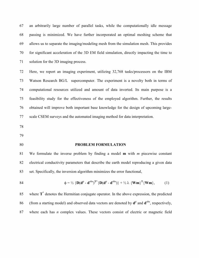
The 3D imaging experiment we present here demonstrates the above mentioned points. 238
The data were acquired offshore of South America. The sail lines and 23 detector locations 239
on a 40×40 km2 grid used for subsurface conductivity mapping are shown in Figure 2. 240
Data was collected from nearly 1 million binned transmitter sites along the shown sail 241
lines. Obviously, this amount of data cannot be treated with the current inversion 242
methodology even with a massively parallel implementation. Every source treated by the 243
imaging algorithm requires a forward simulation, an adjoint computation, and two or more 244
additional simulations for step control for each non-linear inversion update. To efficiently 245
deal with this data volume, we employ reciprocity. The positions of the real CSEM 246
transmitter along the sail line become the computational receiver profiles, and the real 247
CSEM detectors on the seafloor become computational sources, referred to as sources in 248
the following. 249

The equivalent reciprocal problem involves 951,423 data points and 207 effective sources, 250
since there are 23 source locations with three polarizations and each operating at the three 251
discrete excitation frequencies 0.125, 0.25, and 0.5 Hz. Each effective transmitter is 252
polarized according to the antenna orientation of its corresponding detector. The exact 253
seafloor detector orientations were determined by analyzing the data polarizations and 254
phase reversals with respect to the source sail lines. Data processing involves binning in 255
time, followed by spectral decomposition and spatial filtering. Timing errors were 256
removed by forcing the data phases to match the frequency-offset scaling behavior 257
appropriate to solutions of Maxwell's equations. 258
The survey layout in Figure 2 contains different transmitter-receiver configurations to be 259
considered, as is illustrated in the upper Figure 2. For the transmitter sail line position with 260
respect to a given detector on the sea bottom, we consider the so-called overflight (a) 261
configuration, where the sail line is directly over the detector. In the broadside 262
configuration (b), the towed transmitter passes at an offset ∆y to one side of the detector. 263
Three components are recorded by the detector’s receiver antennas: inline horizontal (Ex), 264
perpendicular horizontal (Ey), and vertical (Ez) electric fields. 265
A starting model is necessary to launch the inversion process and resolve some final issues 266
associated with phase components in the data. It is obviously favorable to achieve 267
minimum data misfits with the starting model. Therefore, the model used has been 268
constructed from knowledge of the sea bottom bathymetry, the seawater electrical 269
conductivity-versus-depth profile, and 1D inversion of the amplitude components of the 270
common-receiver gathers, based on the inline overflight measurement configuration (Exi). 271

The resulting 1D models were then refined by comparing selected simulation results with 272
field observations. To accommodate all sail lines and detector sites in the model, a large 273
parameterization was required for Ωm. To model bathymetry, the minimum required 274
spatial grid sampling interval ∆ is kept constant with ∆=125 m for the horizontal, x and y, 275
coordinates, while it ranges from 50 to 200 m in z. This amounts to 403 nodes along x and 276
y, and 173 nodes vertically, and thus approximately 27.8 million model cells. 277
To restrict the size of the simulation grid for each source activation, we have assigned each 278
a separate mesh. Both mesh size and spatial grid sampling rate are based on skin depth 279
estimations. The skin depth δ, a commonly used constant in EM applications, is defined as 280
the depth below the surface of a conductor (in our case at the transmitter location) at which 281
the current density decays to 1/e (about 0.37) of the surface current density. Using the 282
approximation, 283
fbσδ /503= , 284
mesh intervals depend on the source excitation frequency f and the background 285
conductivity σb of the employed starting model. Horizontal mesh size is based on ten skin 286
depths from the source midpoint, assuming σb=0.5 S/m; the resulting mesh ranges were of 287
sufficient size to accommodate the specific sail lines of data assigned to the effective 288
sources. The horizontal spatial grid sampling intervals vary with frequency, ∆=250, 200, 289
and 125 m, for the frequencies f=0.125, 0.25, and 0.5 Hz, respectively. The vertical 290
meshing was identical to that employed in the modeling mesh in order to honor the 291
bathymetry. With these considerations, we were able to reduce the size of the simulation 292

meshes significantly; the number of x and y grid nodes both ranged from 128 to 162. 293
Solution accuracy was verified against solutions where Ωs=Ωm. 294
A maximum of 256 Mbytes of memory per task was available on BG/L. The largest 295
memory requirement results from temporary storage of the forward solutions within one 296
inversion iteration. To stay within the machine limits each simulation grid was distributed 297
across a local communicator size of 512 processors, relying on the inter-processor 298
bandwidth to support the BiCG/QMR solves. Sixty-four local communicators were then 299
used to distribute the 207 effective sources and its associated data. Thus the total number 300
of tasks employed in the imaging experiment was 32,768. Disk IO and file system 301
performance were minor concerns, as the generated image output was relatively modest, 302
approximately 2.5 Gbytes per inversion update, which was written to disk in parallel using 303
512 tasks. Data output at each inversion iteration consisted of predicted and observed 304
measurements with a total file size of 170 Mbytes. A lead task within the global 305
communicator was assigned to dump the data output after each inversion update. 306
Prior to the actual imaging experiment, performance tests were carried out. Base line 307
evaluation involved an inversion where the large model grid (size 403×403×173 nodes) 308
represented the simulation grid for each source. 309
1) The job performance using 32 MPI tasks completed on BG/L (CPU speed 700 310
MHz) and an Intel (Pentium 4, CPU speed 2.6 GHz) cluster with Gigabit Ethernet 311
fabric was compared. A forward solution used 25 sec per 100 QMR iterations on 312
BG/L, compared to 23 sec on the Intel P4 platform. The computational burden of 313
the QMR solver is dominated by complex double precision matrix-vector 314

multiplications with indexed memory access. BG/L’s 64-bit IBM Power 315
architecture is designed for floating point operations achieving an efficient memory 316
access. Profiling shows that for our application the architecture compensates for 317
BG/L’s lower processor speed. 318
2) Workload scalability tests revealed a linear QMR solution time decrease up to a 319
number of 4096 tasks. 320
3) A 1024-task job on BG/L showed that the communication averaged to about 25 % 321
of the total solution time per inversion iteration. The distribution of the 322
communication overhead is as follows. Collective communications within GC are 323
mainly global reduction operations, and amount to about 50% with typical message 324
sizes of 16 Bytes. Point-to-point blocking message passing within LC: 20 % with 325
30 Kbytes average message size. Barrier synchronization: 30%. 326
327
The relatively long idle time due to global barrier synchronization, which is done after 328
each inversion iteration, indicates the importance of a balanced workload distribution 329
among all LCs. The QMR solver convergence behavior depends on the condition number 330
of the FD stiffness matrix K in equation (3), which in turn is governed by the aspect ratio 331
and conductivity contrasts within Ωs. Because the latter changes dynamically with the 332
model updates during an inversion, a faster barrier synchronization would require an 333
adequate sophisticated scheme for dynamically adapting the LC size. 334
Over a 24-hour period, 72 inversion model updates were realized on BG/L and the relative 335
squared error misfit measure was reduced by nearly 67%. Exemplified in Figure 3, good 336

fits, to within the anticipated noise, were obtained for the horizontal and vertical inline 337
electric field overflight data, Exi (a) and Ez
i (b), as well for the horizontal perpendicular and 338
vertical broadside electric fields, Eyb (c) and Ez
b (d). We observed that the major residual 339
misfits originate from the broadside inline components, Exb (e,f). 340
The average resistivity computed over three depth ranges for solution 72 is shown in 341
Figure 4. The sea bottom defines the depth z=0. Inspection of the images shows enhanced 342
resistivity in the southern model section for depths below 1500 m. Such is also observed 343
broadside of the sail lines, for the depth range 0-1500 m. Along the sail lines, however, 344
little to no resistivity enhancement is observed and the imaged resistivity volume contains 345
an unacceptable acquisition overprint. A possible explanation for this outcome is the 346
inconsistencies observed in fitting the in-line component of the broadside data compared 347
to other data components. This is particularly true of inline overflight data. Clearly, the 348
overflight data will be most sensitive to resistivity variations along the sail lines, while 349
broadside data are more sensitive to resistivity variations off the sail lines. One possibility 350
for the enhanced resistivity observed off the sail lines arises from the inversion algorithm’s 351
attempt to fit the inline broadside data. Enhanced resistivity amplifies the broadside inline 352
model data, reducing the mismatch between observed and predicted data. Nevertheless, it 353
was still not possible to achieve acceptable data fits indicating a systematic bias in the 354
underlying assumptions employed in the inversion processing. 355
One critical assumption in this inversion was that the conductivity is isotropic; 356
conductivity within a cell does not vary with direction. However, it is well known within 357
sedimentary rocks that fine grain bedding planes can induce the rocks to exhibit transverse 358

electrical anisotropy [13 and 14]. In addition, parallel interbedding of rocks with different 359
conductivities can lead to anisotropic behavior. Thus, the conductivity can be expected to 360
depend strongly on directions, parallel and perpendicular to the bedding planes. In the 361
context of marine CSEM, [15] showed that the effects of electrical anisotropy can produce 362
significant anomalies, even as large as target reservoir responses, and a consensus is now 363
emerging that electrical anisotropy plays a bigger factor in influencing marine CSEM 364
measurement than previously believed. 365
Two tests were carried out to verify the importance of anisotropy. First, to test the degree 366
to which electrical anisotropy is affecting the broadside inline data, and to what lesser 367
extent it influences the overflight and broadside perpendicular and vertical data, we 368
repeated the initial stage of the inversion process. This involved an anisotropic model with 369
the vertical conductivity fixed at the conductivity used in the initial isotropic inversion and 370
the horizontal conductivity set to three times the vertical conductivity below the water 371
bottom. A sampling of the results is shown in Figure 5, confirming that the data are very 372
likely significantly more consistent with an anisotropic conductivity model than with an 373
isotropic one. Furthermore, we rerun two inversions with a subset of the data, comprising 374
36 effective transmitters. Using the same isotropic starting model, the inversions differed 375
by using an isotropic and anisotropic model parameterization. After 62 iterations, the 376
anisotropic model achieved a final data fit, which was by 27 % lower, compared to the 377
isotropic result. A complete anisotropic inversion of these data has yet to be carried out. 378
379
380

CONCLUSIONS 381
We have made significant progress in reducing the computational demands of large-scale 382
3D EM imaging problems. Exploiting multiple levels of parallelism over the data and 383
model spaces and utilizing different meshing for field simulation and imaging provides a 384
capability to solve large 3D imaging problems that cannot be addressed otherwise in a 385
timely manner. 386
Results of the Blue Gene/L experiment for this offshore data showed that the broadside 387
inline component data displays a systematic bias that is most likely attributable to 388
conductivity anisotropy between the vertical and horizontal directions. The other field 389
components were satisfactorily fit by an isotropic model, showing that these field 390
components are significantly less sensitive to this kind of anisotropy. The speed at which 391
the Blue Gene/L supercomputer delivered this result is essential to the time frame in which 392
the exploration process is conducted. This work provides motivation to extend the 3D 393
conductivity imaging methodology to the anisotropic situation. 394
395
ACKNOWLEDGMENTS 396
The authors gratefully acknowledge donation of Blue Gene/L computing resources by the 397
IBM Corporation. Base funding for this work was provided by the ExxonMobil 398
Corporation and the United States Department of Energy, Office of Basic Energy 399
Sciences, under contract DE-AC02-05CH11231. We also wish to thank the German 400
Alexander-von-Humboldt Foundation for support of Michael Commer through a Feodor-401
Lynen research fellowship. We wish to acknowledge the contributions of our colleague 402

Dr. Xinyou Lu, who provided the 1D inversion code and the contributions of our 403
colleagues Dr. Dmitriy A. Pavlov and Dr. Charlie Jing of ExxonMobil who contributed 404
many useful insights into the behavior of CSEM data in anisotropic conductivity models. 405
406
407
REFERENCES 408
1. T. Eidesmo, S. Ellingsgrud, L. M. MacGregor, S. Constable, M. C. Sinha, S. Johansen, 409
F. N. Kong, and H. Westerdahl, “Sea Bed Logging (SBL), a new method for remote 410
and direct identification of hydrocarbon filled layers in deepwater,” First Break, 20, No. 3, 411
144-152 (March 2002). 412
413
2. S. Ellingsrud, T. Eidesmo, S. Johansen, M. C. Sinha, L. M. MacGregor, and S. 414
Constable, “Remote sensing of hydrocarbon layers by seabed logging (SBL): Results from 415
a cruise offshore Angola,” The Leading Edge, 21, No. 10, 972-982 (October 2002). 416
417
3. L. M. MacGregor and M. C. Sinha, “Use of marine controlled source electromagnetic 418
sounding for sub-basalt exploration,” Geophysical Prospecting, 48, No. 6, 1091-1106 419
(November 2000). 420
4. L. J. Srnka, J. J. Carazzone, M. S. Ephron, and E. A. Eriksen, “Remote reservoir 421
resistivity mapping,” The Leading Edge, 25, No. 8, 972-975 (August 2006). 422
423

5. S. Constable, “Marine electromagnetic methods – A new tool for offshore exploration,” 424
The Leading Edge, 25, No. 4, 438-444 (April 2006). 425
426
6. D. L. Alumbaugh, G. A. Newman, L. Prevost, and J. Shadid, “Three-dimensional, 427
wideband electromagnetic modeling on massively parallel computers,” Radio Science. 31, 428
No. 1, 1-23 (January-February 1996). 429
430
7. G. A. Newman and P. T. Boggs, “Solution accelerators for large-scale three-431
dimensional electromagnetic inverse problems,” Inverse Problems, 20, doi:10.1088/0266-432
5611/20/6/S10, S151-S171 (2004). 433
8. M. Commer and G. A. Newman, “Large scale 3D EM inversion using optimized 434
simulation grids non-conformal to the model space,” Exp. Abstr. Soc. Expl. Geophys., 25, 435
760-764 (2006). 436
9. G. A. Newman and D. L. Alumbaugh, “Three-dimensional massively parallel 437
electromagnetic inversion - Part I. Theory,” Geophys. J. Int., 128, No. 2, 345-354 438
(February 1997). 439
440
10. S. Moskow, V. Druskin, T. Habashy, P. Lee, and S. Davdychewa, “A finite difference 441
scheme for elliptic equations with rough coefficients using a Cartesian grid nonconforming 442
to interfaces,” SIAM J. Number. Anal., 36, No. 2, 442-464 (February 1999). 443

11. J. J. Carazzone, O. M. Burtz, K. E. Green, and D. A. Pavlov, “Three dimensional 444
imaging of marine CSEM data,” Exp. Abstr. Soc. Expl. Geophys., 24, 575-578 (2005). 445
12. K. E. Green, O. M. Burtz, L. A. Wahrmund, T. Clee, I. Gallegos, C. Xia, G. Zelewski, 446
A. A. Martinez, M. J. Stiver, C. M. Rodriguez, and J. Zhang, “R3M Case studies: 447
detecting reservoir resistivity in complex settings,” Exp. Abstr. Soc. Expl. Geophys., 24, 448
572-574 (2005). 449
13. J. D. Klein, P. R. Martin, and D. F. Allen, “The petrophysics of electrically anisotropic 450
reservoirs,” Trans. Soc. Petrol. Well-Log Analysts (SPWLA); 36th Ann. Logging Symp., 451
(1995). 452
453
14. J. Zhao, D. Zhou, X. Li, R. Chen, and C. Yang, “Laboratory measurements and 454
applications of anisotropy parameters of rocks,” Trans. Soc. Petrol. Well-Log Analysts 455
(SPWLA); 35th Ann. Logging Symp., (1994). 456
15. G. M. Hoversten, G. A. Newman, N. Geier, and G. Flanagan, G., “3D modeling of a 457
deepwater EM exploration survey,” Geophysics, 71, No. 5, G239-G248 (September-458
October 2006) . 459
460
461
462

463
Figure captions 464
Figure 1. Illustration of the conductivity averaging scheme of equation (4) in two 465
dimensions. 466
Figure 2. Layout of the sail lines (red and blue) and 23 detector locations (crosses) on the 467
sea bottom for the offshore CSEM survey. Contained survey configurations are illustrated 468
in the upper figure. Bathymetry is given in meters below sea level. The example data 469
shown in this paper corresponds to the transmitter-detector arrays marked in blue. 470
Figure 3. Six selected plots of overflight and broadside electric field data amplitudes 471
(black curves) versus the transmitter offset projected onto the profile lines shown in Figure 472
2. Shown are data fits produced by the starting model (red) and for iteration 72 (blue). 473
Figure 4. Average resistivity computed over three depth ranges for solution 72: a) Water 474
bottom to 500 m below mud line (BML), b) interval 500 to 1500 m BML, c) interval 1500 475
to 2500 m BML. Resistivity is rendered on a base 10 log scale. 476
Figure 5. Six selected plots of overflight and broadside electric field data amplitudes 477
(black curves) versus the transmitter offset projected onto the profile. Shown are data fits 478
produced by a starting model with isotropic (red) and anisotropic (blue) electrical 479
conductivity. 480
481

482
483
484
Fig. 1 485
486
Fig. 2 487

488
Fig. 3 489
490
491
492

a) 493
494
b) 495
496
c) 497
498
Fig. 4 499
1 2 log ρ (Ω.m)

500
Fig. 5 501
502
503
504

Michael Commer 505
Lawrence Berkeley National Laboratories, Berkeley, CA 94720 ([email protected]). 506
M. Commer received his Ph.D. degree in Geophysics from the University of Cologne, 507
Germany. His research focused on transient electromagnetic modeling and inversion and 508
was awarded the German Klaus-Liebrecht prize for outstanding dissertations. Current 509
research areas include large-scale time- and frequency domain modeling and data 510
inversion using massively parallel computers. Since 2004, Dr. Commer has been 511
employed with LBNL, where he initially started as a post-doctoral fellow supported by the 512
German Alexander-von-Humboldt foundation. 513
514
Gregory A. Newman 515
Lawrence Berkeley National Laboratories, Berkeley, CA 94720 ([email protected]). 516
Gregory Newman received his Ph.D. degree in Geophysics from the University of Utah in 517
1987. He is an expert in large scale electromagnetic field modeling and inversion, with an 518
emphasis on massively parallel implementations. In 2004, Dr. Newman accepted a Senior 519
Scientist appointment within the Earth Sciences Division at Lawrence Berkeley National 520
Laboratory. Previously he has been associated with Sandia National Laboratories and 521
Institute of Geophysics and Meteorology, Cologne Germany. 522
523
James J. Carazzone 524
ExxonMobil Upstream Research Company, Houston, TX 77252 525

([email protected]). James Carazzone received his Ph.D. degree in 526
Physics from Harvard University in 1975 and had two post-doctoral appointments in the 527
areas of elementary particle physics and quantum field theory at the Fermi National 528
Accelerator Laboratory and at the Institute for Advanced Study at Princeton. In 1978 he 529
joined Exxon’s upstream research organization where he has worked ever since in the 530
areas of seismic and electromagnetic modeling and inversion applied to hydrocarbon 531
exploration. Dr. Carazzone is a member of the Society of Exploration Geophysicists and of 532
the European Association of Geophysicists and Engineers. 533
534
Thomas A. Dickens 535
ExxonMobil Upstream Research Company, Houston, TX 77252 536
([email protected]). Thomas Dickens received a B.S. in Physics from the 537
University of Virginia (1981) and a Ph.D. in Physics from Princeton University in 1987, 538
where he was awarded the Joseph Henry Prize. From 1987-1990 he was employed by MIT 539
Lincoln Laboratory, where he worked on synthetic aperture radar and infrared imaging 540
techniques. He joined Exxon Production Research (now ExxonMobil Upstream Research) 541
in 1990, and has performed research in the areas of tomography, parallel computing, and 542
imaging of complex structures, anisotropic depth migration, and electromagnetic 543
inversion. His current research interests include seismic and electromagnetic imaging, 544
signal processing, and modeling. He is a member of SEG, APS, and SIAM. 545
546
547

548
549
Kenneth E. Green 550
ExxonMobil Upstream Research Company, Houston, TX 77252 551
([email protected]). Ken Green received his undergraduate degree in 552
Geophysics from MIT in 1974 and a doctorate in Oceanography from the MIT - Woods 553
Hole Oceanographic Institution in 1980. He joined the Geoscience function at Exxon 554
Production Research Company in 1980. His work at ExxonMobil has covered many 555
aspects of exploration in basin hydrocarbon systems including the subsurface visualization 556
of earth resistivity volumes applied to oil and gas migration, entrapment and production. 557
Ken is a member of the Society of Exploration Geophysicists. 558
559
Leslie A. Wahrmund 560
ExxonMobil Upstream Research Company, Houston, TX 77252 561
([email protected]). Leslie Wahrmund received her B.A. degree in 562
Geological Sciences from the University of California at Santa Barbara, and her Ph.D in 563
Geology from the University of Texas at Austin. She has worked at Exxon Production 564
Research (now ExxonMobil Upstream Research) since 1991, primarily in seismic 565
interpretation and seismic attribute analysis. She has worked on integration and 566
interpretation of CSEM data since 2003. 567
568
Dennis E. Willen 569

ExxonMobil Upstream Research Company, Houston, TX 77252 570
([email protected]). Dr. Willen joined Exxon Production Research 571
Company in 1980, after receiving his Ph.D. in Physics from the University of Illinois. 572
Since then he has worked in several areas of exploration geophysics including seismic 573
imaging, near-surface effects, converted waves, well logging, parallel computing, and 574
electromagnetic methods. He is a member of the Society of Exploration Geophysicists 575
and the International Trumpet Guild. 576
577
Janet Shiu 578
IBM Deep Computing, Two Riverway, Houston, Texas 77056 579
([email protected]). Dr. Shiu received her Ph.D. degree in Physics from University of 580
Pittsburgh. Dr. Shiu was an assistant professor at Old Dominion University, and a 581
principal investigator of research grants from NASA Langley Research Center where her 582
research focus were in the area of high power lasers for space application. Since 1985, Dr. 583
Shiu has been employed with Cray Research Inc., SGI, and Exxon Upstream Technical 584
Company in technical support of High Performance Computing. Dr. Shiu joined IBM in 585
1999, and is a member of IBM Deep Computing Technical Team. 586
587