AcceptedPreprint typeset using LATEX style AASTeX6 v. 1.0

SUB-CHANDRASEKHAR-MASS WHITE DWARF DETONATIONS REVISITED

Ken J. Shen1,2, Daniel Kasen1,2,3, Broxton J. Miles4, and Dean M. Townsley4

1Department of Astronomy and Theoretical Astrophysics Center, University of California, Berkeley, CA, USA; kenshen@astro.berkeley.edu2Lawrence Berkeley National Laboratory, Berkeley, CA, USA3Department of Physics, University of California, Berkeley, CA, USA4Department of Physics and Astronomy, University of Alabama, Tuscaloosa, AL, USA

ABSTRACT

The detonation of a sub-Chandrasekhar-mass white dwarf (WD) has emerged as one of the most

promising Type Ia supernova (SN Ia) progenitor scenarios. Recent studies have suggested that the

rapid transfer of a very small amount of helium from one WD to another is sufficient to ignite a

helium shell detonation that subsequently triggers a carbon core detonation, yielding a “dynamically

driven double degenerate double detonation” SN Ia. Because the helium shell that surrounds the core

explosion is so minimal, this scenario approaches the limiting case of a bare C/O WD detonation.

Motivated by discrepancies in previous literature and by a recent need for detailed nucleosynthetic

data, we revisit simulations of naked C/O WD detonations in this paper. We disagree to some extent

with the nucleosynthetic results of previous work on sub-Chandrasekhar-mass bare C/O WD detona-

tions; e.g., we find that a median-brightness SN Ia is produced by the detonation of a 1.0M� WD

instead of a more massive and rarer 1.1M� WD. The neutron-rich nucleosynthesis in our simulations

agrees broadly with some observational constraints, although tensions remain with others. There are

also discrepancies related to the velocities of the outer ejecta and light curve shapes, but overall our

synthetic light curves and spectra are roughly consistent with observations. We are hopeful that fu-

ture multi-dimensional simulations will resolve these issues and further bolster the dynamically driven

double degenerate double detonation scenario’s potential to explain most SNe Ia.

Keywords: binaries: close— nuclear reactions, nucleosynthesis, abundances— radiative transfer—

supernovae: general— white dwarfs

1. INTRODUCTION

The nature of Type Ia supernova (SN Ia) progeni-

tors remains one of the enduring mysteries of astro-

physics (for recent reviews, see Hillebrandt et al. 2013

and Maoz et al. 2014). For decades, many researchers

favored a scenario involving a C/O white dwarf (WD)

whose mass approaches the Chandrasekhar limit via sta-

ble hydrogen-rich accretion from a non-degenerate com-

panion (Whelan & Iben 1973; Nomoto 1982b) or in an

unstable merger with another C/O WD (Iben & Tu-

tukov 1984; Webbink 1984). Carbon fusion at the cen-

ter of the WD would then lead to a phase of convective

simmering, followed by the birth of a deflagration, a

transition to a detonation, and subsequently, a SN Ia

explosion (e.g., Khokhlov et al. 1997; Plewa et al. 2004;

Seitenzahl et al. 2013b).

However, growing constraints from recent theoretical

and observational work have increased persisting doubts

that the Chandrasekhar-mass (MCh) scenario is respon-

sible for the bulk of SNe Ia (e.g., Leonard 2007; Shen

& Bildsten 2007; Kerzendorf et al. 2009; Ruiter et al.

2009; Kasen 2010; Bloom et al. 2012; Schaefer & Pag-

notta 2012; Woods & Gilfanov 2013; Scalzo et al. 2014;

Johansson et al. 2016; Dhawan et al. 2017). Increased

attention is being paid to alternative solutions, chief

among them the double detonation scenario. In its ear-

liest incarnations (Woosley et al. 1986; Nomoto 1982a;

Livne 1990), this scenario invoked accretion from a non-

degenerate helium-burning star onto a C/O WD, which

leads to a ∼ 0.1M� helium shell that ignites, begins to

convect, and then detonates. The helium shell detona-

tion then triggers a detonation in the sub-MCh C/O core

via a direct edge-lit detonation or via shock convergence

near the center. However, the helium detonation in the

massive shells of these early models produced 56Ni and

other iron-group elements in the outer regions of the

SN ejecta, which presented problems when compared to

observations (Hoflich & Khokhlov 1996; Nugent et al.

1997).

In recent years, the realization that stable accretion

from helium WD donors yields much smaller helium

shells at ignition due to the higher accretion rates (Bild-

arX

iv:1

706.

0189

8v3

[as

tro-

ph.H

E]

30

Jan

2018

2 SHEN ET AL.

sten et al. 2007; Shen & Bildsten 2009), coupled with the

problems besetting MCh scenarios, motivated a resur-

gence of double detonation studies focused on the explo-

sion of sub-MCh WDs (Fink et al. 2007, 2010; Kromer

et al. 2010; Woosley & Kasen 2011; Shen & Bildsten

2014). In parallel work, studies of unstable double WD

mergers uncovered the possibility that helium could det-

onate as it was transferred during the dynamical phase

of the merger (Guillochon et al. 2010; Raskin et al. 2012;

Pakmor et al. 2013; Moll et al. 2014; Tanikawa et al.

2015). This scenario was made even more attractive due

to work that showed that including a large nuclear reac-

tion network and realistic C/O pollution in the helium

shell drastically reduces the minimum hotspot size and

shell mass for helium detonation initiation and propa-

gation (Shen & Moore 2014).

Observational studies have begun to narrow the highly

uncertain double WD interaction rate, finding rough

agreement with binary population synthesis calculations

(e.g., Ruiter et al. 2011; Toonen et al. 2017). A recent

observational estimate (Maoz & Hallakoun 2017) finds

that the rate of double WDs coming into mass transfer

contact is ∼ 10 times the SN Ia rate. Not all of these bi-

naries necessarily lead to double WD mergers, but Shen

(2015) introduced the possibility that all double WD

systems do indeed merge unstably due to dynamical fric-

tion during the initial phases of stable hydrogen- and

helium-rich mass transfer. Thus, double WD binaries

have the potential to explain all SNe Ia if just ∼ 10% of

double WD mergers lead to SNe Ia via double detona-

tions (or via direct carbon ignition; Pakmor et al. 2010,

2011, 2012; Kashyap et al. 2015). Furthermore, prompt

detonations in merging double WD binaries also have

the capacity to explain the evolution of the SN Ia lumi-

nosity function (Shen et al. 2017).

Sim et al. (2010) provided a baseline for radiative

transfer simulations of double detonation SNe Ia by cal-

culating the explosion and appearance of a bare C/O

WD core with no overlying helium shell. They found

reasonable agreement with observations of SNe Ia, both

in terms of light curves and spectra. However, recent

work by Moll et al. (2014) included a set of hydrodynam-

ical explosions of bare C/O WDs that disagreed with the

nucleosynthetic results of Sim et al. (2010). Moreover,

recent observational results concerning neutron-rich iso-

topes in SNe Ia (e.g., Seitenzahl et al. 2013a; Yamaguchi

et al. 2015; Dimitriadis et al. 2017) have been claimed

as evidence against sub-MCh explosions, but compre-

hensive in-depth studies of nucleosynthetic abundances

in sub-MCh detonations do not yet exist in the literature

for comparison to these observations.

Motivated by the disagreement in previous work and

by the need for detailed nucleosynthetic data, we re-

visit simplified simulations of spherically symmetric bare

C/O WD detonations in this paper. While recent stud-

ies have performed hydrodynamical and radiative trans-

fer simulations with multi-dimensional helium shell ig-

nitions (e.g., Fink et al. 2007, 2010; Kromer et al. 2010;

Sim et al. 2012; Moll & Woosley 2013), their use of rela-

tively massive helium shells yielded significant amounts

of iron-group elements in the helium detonation ashes,

which continues to be a vexing issue for obtaining spec-

troscopically normal SNe Ia from these models. The

much smaller helium shells at ignition found by Shen &

Moore (2014) suggest that the study of one-dimensional

baseline bare WD core detonations with no helium shell

is still informative. Future work will continue the devel-

opment of double detonation models by including these

very low mass helium shells in multi-dimensional simu-

lations.

We begin in §2 by describing our method for artifi-

cially broadening detonations in WDs into structures

that are spatially resolved on our numerical grid. In

§3, we detail our nucleosynthetic results for a suite of

80 post-processed simulations, focusing on bulk yields

in §3.1 and on neutron-rich nucleosynthesis in §3.2. We

perform radiative transfer simulations and demonstrate

qualitative agreement with light curves (§4.1) and spec-

tra (§4.2) of observed SNe Ia, and we conclude with

avenues for future research in §5.

2. SIMULATION DETAILS

In this section, we describe our procedure for setting

up, running, and post-processing our reactive hydrody-

namic simulations. We begin by calculating the initial

conditions for our white dwarfs (WDs) with the stellar

evolution code MESA1 (Paxton et al. 2011, 2013, 2015).

We construct WDs with masses of 0.8, 0.85, 0.9, 1.0,

and 1.1M� and uniform compositions of 50/50 or 30/70C/O by mass. The WDs are initially hot and are allowed

to cool until their central temperatures reach 3× 107 K.

The density profiles of these 10 models are then used

as initial conditions for our FLASH2 simulations (Fryxell

et al. 2000; Dubey et al. 2009). FLASH and MESA use

the same equation of state for most of the relevant pa-

rameter space (Timmes & Swesty 2000), but there is

still a small deviation from hydrostatic balance in the

outer regions of the WD after mapping to FLASH. How-

ever, any spurious velocities are erased after the deto-

nation passes. Each one-dimensional spherically sym-

metric simulation has a domain size of 1011 cm and 19

levels of adaptive mesh refinement for a minimum cell

1 http://mesa.sourceforge.net, version 8845; default optionsused unless otherwise noted.

2 http://flash.uchicago.edu, version 4.2.2; default optionsused unless otherwise noted.

Sub-MCh WD detonations 3

size of 4.8 × 104 cm within the WD. The criteria for

refinement are based on the gradients of pressure, den-

sity, and temperature using FLASH’s default thresholds.

At a radius initially just outside the WD’s surface, the

minimum allowed cell size increases by a factor of two

and continues to increase linearly with radius beyond

this location. This limits the amount of computational

time spent following the shock that propagates outwards

into the ambient medium after the detonation passes

through the WD. Additionally, the maximum level of

refinement in the innermost 107 cm is reduced by four

levels so that inwardly propagating shocks do not limit

the global timestep as they converge towards the center

and increase their velocity.

The C/O ratio of the WD in FLASH is set to match

the MESA model from which it came. Furthermore, we

include four different metallicities for our initial models:

0, 0.5, 1, and 2Z�, which we approximate by includ-

ing 22Ne, the stopping point for CNO isotopes following

helium-burning, and 56Fe at mass fractions of X22Ne =

0, 0.005, 0.01, and 0.02 with X56Fe = 0.1X22Ne. The

ambient medium surrounding the WD is initialized with

a density and temperature of 10−3 g cm−3 and 106 K.

We enable monopole gravity and nuclear burning. Burn-

ing in physical detonations occurs behind the nearly in-

finitesimally thin shock front, so reactions in FLASH are

disabled within shocks by default to avoid unphysical

detonation structures. Fryxell et al. (1989) showed that

an Eulerian piecewise parabolic method hydrodynam-

ics code with reactions disabled within shocks produces

the correct detonation speeds even for unresolved burn-

ing, as well as avoiding a potential artificial deflagration

caused by numerical mixing at the shock front. See Ap-

pendix A of Townsley et al. (2016) for a more detailed

discussion.

We have extended FLASH’s nuclear burning capabili-

ties by incorporating an interface to MESA’s nuclear burn-

ing module, which enables the ability to construct an

arbitrary nuclear reaction network. For our hydrody-

namic simulations, we use a 41-isotope network com-

prised of neutrons, 1H, 4He, 11B, 12C, 13−14N, 16−17O,20,22Ne, 23Na, 24−26Mg, 27Al, 28−30Si, 30−31P, 31−32S,35Cl, 36−39Ar, 39K, 40Ca, 43Sc, 44Ti, 47V, 48Cr, 51Mn,52,56Fe, 55Co, and 56,58−59Ni, with 190 interlinking re-

actions from JINA’s REACLIB (Cyburt et al. 2010). For

the relevant detonation conditions in C/O-rich mate-

rial, this network yields errors of at most a few per-

cent in the energy release. Note that the above net-

work is only tailored to track accurate energy release

but not accurate isotopic abundances. In order to more

precisely calculate abundances, we include tracer parti-

cles for post-processing, which track the radius, velocity,

density, and temperature and are evenly spaced every

5× 106 cm throughout the WD.

The detonation is ignited at the center of the WD by

initializing a hotspot of radius 4×107 cm that has a lin-

ear temperature gradient with a central temperature of

2× 109 K and an outer temperature of 1.2× 109 K. The

temperature just outside the hotspot and throughout

the rest of the WD is set to a constant 3 × 107 K; note

that the value of the initial WD temperature is unimpor-

tant because post-shock temperatures are ∼ 100 times

higher. The 4× 107 cm hotspot is much larger than the

minimum detonatable regions found by previous work

(Arnett & Livne 1994; Niemeyer & Woosley 1997; Ropke

et al. 2007; Seitenzahl et al. 2009a) but is necessary due

to the burning limiter we describe below. We have con-

firmed that our results are insensitive to the size of the

hotspot, which is reasonable because inaccurate nucle-

osynthesis due to the temperature perturbation will be

confined to the hotspot, which corresponds to a cen-

tral mass of just 0.0014, 0.0018, 0.0025, 0.0045, and

0.0088M� for our 0.8, 0.85, 0.9, 1.0, and 1.1M� 50/50

C/O WDs.

One goal of our work is to ensure that we are capturing

the relevant physics by spatially resolving the reaction

front structure in our simulations. However, C/O deto-

nations have lengthscales 10−104 cm at our densities of

interest and have thus been previously followed with a

level set or progress variable method (e.g., Calder et al.

2007; Sim et al. 2010; Seitenzahl et al. 2013b; Townsley

et al. 2016). We overcome this obstacle by artificially

broadening the detonation, similar in spirit to previ-

ous studies that thicken deflagration fronts (Khokhlov

1995; Calder et al. 2007; Townsley et al. 2016), and

subsequently testing our resolved simulations for con-

vergence. We broaden the detonation by introducing a

limit to the relative amount the temperature can change

within each cell in one timestep due to nuclear burning,

|∆ lnT |max, similar to the method employed by Kushnir

et al. (2013). For our primary simulations we choose

|∆ lnT |max = 0.04, motivated by the convergence stud-

ies detailed in §2.1.

Reactions and hydrodynamics in FLASH are computed

in an operator-split fashion. Between each computation

of the hydrodynamic evolution during a time ∆thydro,

the timestep determined by the Courant condition

(Fryxell et al. 2000), a temporally resolved integration

of the reactions is performed in each cell with an initial

integration time of ∆treact = ∆thydro. From the entropy

equation, the relative change in temperature is ∆ lnT ∼ε∆treact/cV T , where ε is the average energy generation

rate over the timestep ∆treact, and cV is the specific heat

at constant volume. If |∆ lnT | > |∆ lnT |max in a cell,

the burning integration time, ∆treact, is reduced to the

appropriate value via a Newton-Raphson iteration while

leaving ∆thydro unchanged. The burning integration is

re-run for each iteration in order to yield consistent ener-

4 SHEN ET AL.

getics and abundance changes. This limiting procedure

can also be thought of as integrating the reactions for

the full hydrodynamic timestep, ∆thydro, but with all

the reaction rates reduced by the multiplicative factor

∆treact/∆thydro.

Simulations are evolved for 10 s, after which the

tracer particles’ density and temperature histories are

post-processed with MESA’s one zone burner. We em-

ploy a 205-isotope network that includes neutrons,1−2H, 3−4He, 6−7Li, 7,9−10Be, 8,10−11B, 12−13C, 13−16N,15−19O, 17−20F, 19−23Ne, 21−24Na, 23−27Mg, 25−28Al,27−33Si, 30−34P, 31−37S, 35−38Cl, 35−41Ar, 39−44K,39−49Ca, 43−51Sc, 43−54Ti, 47−56V, 47−58Cr, 51−56Mn,51−62Fe, 54−62Co, 54−62Ni, 58−66Cu, 59−66Zn, 59−66Ga,

and 59−66Ge and interlinking reactions from JINA’s

REACLIB (Cyburt et al. 2010). We post-process each

of our 40 hydrodynamic simulations with two different

normalizations of the 12C+16O reaction rate (1 and 0.1

times the default rate; see §3.2.4 for the motivation be-

hind this variation) for a total of 80 post-processed re-

sults.

2.1. Convergence studies

In this section, we demonstrate the convergence of our

results as we increase the resolution in our simulations

for a set of 1.0M� 50/50 C/O solar metallicity WD

detonations. Note that since the physical burning scales

are not resolved by many orders of magnitude, conver-

gence does not imply correctness, only that our thick-

ening scheme is numerically consistent over the range

of grid scales used here. Verification of yields against

resolved calculations will be the topic of future work.

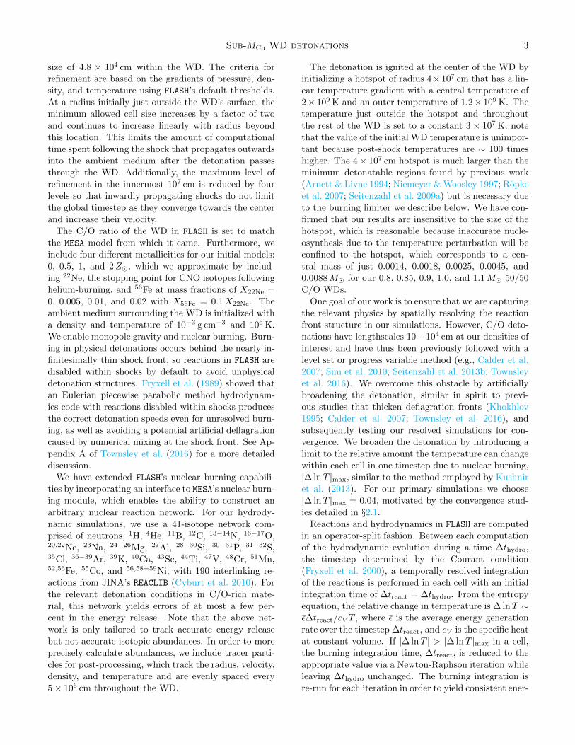
Figure 1 shows synthesized masses of 56Ni and

intermediate-mass elements (IMEs; defined as having

charges 11 ≤ Z ≤ 20) and the total nuclear energy re-

lease, Enuc, for three sets of hydrodynamic simulations

and three post-processed results vs. the minimum cell

size in the simulation. The dashed lines represent the

hydrodynamic results, which use a 41-isotope network,

and the solid lines show results from post-processing the

same hydrodynamic simulations using a 205-isotope net-

work.

As Figure 1 demonstrates, global values are con-

verged for minimum cell sizes . 105 cm for both the

|∆ lnT |max = 0.02 and 0.04 cases, with relevant quanti-

ties changing by < 1% with a factor of two increase in

resolution. Results for the |∆ lnT |max = 0.08 simulation

do not appear to be fully converged at our highest reso-

lution, which motivates our choice of |∆ lnT |max = 0.04

for all of the production runs in this work.

The bulk nucleosynthetic yields of the hydrodynamic

results without post-processing and the results after

post-processing are discrepant at a 3− 10% level. How-

ever, as previously discussed, the 41-isotope nuclear re-

●●●

0.34

0.36

0.38

MIM

E[M

�]

|∆ lnT |max = 0.02

|∆ lnT |max = 0.04 |∆ lnT |max = 0.080.52

0.54

0.56

M56Ni

[M�

]

Hydrodynamic, 41 isotopesPost-processed, 205 isotopes

5× 104 105 2× 105

1.37

1.38

Minimum cell size [cm]

Enuc

[105

1er

g]

Figure 1. Synthesized IME (top panel) and 56Ni (middlepanel) masses and total nuclear energy release (bottom panel)vs. minimum cell size allowed in the simulation for detona-tions of 1.0M� 50/50 C/O solar metallicity WDs. Dashedlines represent the results from our hydrodynamic simula-tions, which use a 41-isotope network, for a maximum rela-tive temperature change per timestep of |∆ lnT |max = 0.02(thin red dashed), 0.04 (medium blue dashed), and 0.08 (thickyellow dashed). Post-processed results using a 205-isotopenetwork are shown as solid lines for |∆ lnT |max = 0.02 (thinred solid), 0.04 (medium blue solid), and 0.08 (thick yellowsolid). Circles in the top panel show the minimum cell sizesof the convergence study for reference.

action network used in the hydrodynamics simulations

is designed to capture energetics, not isotopic abun-

dances. Thus, the agreement in energetics before and

after post-processing is much better, with only a ' 0.3%

difference. This gives confidence that the tracer parti-cles’ density and temperature histories used in the post-

processing calculation and the resulting nucleosynthetic

abundances are accurate.

2.2. Spatially resolved broadened detonation structure

Our burning limiter allows us to spatially resolve the

artificially broadened detonation structure in our hydro-

dynamic simulations, an example of which is shown in

Figure 2. The top panel shows thermodynamic variable

profiles, and the bottom panel shows profiles of the en-

ergy generation rate normalized to the maximum value,

ε/εmax, and the mass fractions of 11 isotopes as labeled.

The other 30 isotopes comprising the 41-isotope net-

work used in our hydrodynamical simulations do not

reach mass fractions above 10−2 in this plot at this time,

0.24 s after the simulation has begun. The time of the

snapshot is chosen to coincide with when the detonation

reaches the mass coordinate (0.64M� from the center)

Sub-MCh WD detonations 5

ε/εmax

12C

16O

20Ne

28Si

32S

36Ar

40Ca

52Fe

56Ni

55Co

58Ni

105 106 107

10−1

1

Distance behind shock [cm]

Massfraction

san

dε/ε m

ax

P/1024 dyne cm−2

T/109K

ρ/107 g cm−3

02

46

Thermodynam

icvariab

les

Figure 2. Top panel : The pressure, temperature, and den-sity, normalized as labeled, vs. distance behind the shockin a 1.0M� 50/50 C/O WD detonation 0.24 s after the be-ginning of the simulation. Bottom panel : Profiles of massfractions and the normalized energy generation rate, ε/εmax.The other isotopes that do not appear in the panel do notreach mass fractions > 10−2 at this stage of the detonation.

where the 56Ni fraction will equal the 28Si fraction after

the simulation ends.

The density upstream of the detonation at this time is

6.3 × 106 g cm−3. The carbon consumption lengthscale

for a steady state detonation at this density is ∼ 102 cm,

and the lengthscale for an overdriven detonation such

as this is even shorter (Khokhlov 1989; Townsley et al.

2016). Due to the use of our burning limiter, we achieve

a spatially resolved detonation by construction. The

broadened detonation in our simulation has a carbon

consumption lengthscale of ∼ 105 cm, > 10 times longer

than the true lengthscale, and the maximum of the en-

ergy generation rate is several zones behind the shock

front instead of just behind or inside the shock where it

would be located for an unresolved detonation. While

the detonation itself is not physically correct, the con-

vergence study in §2.1 gives us confidence that the major

yields will be relatively unchanged at higher resolutions.

These yields will be verified by comparison to resolved

calculations in future work.

2.3. Ejecta profiles

Figure 3 shows density vs. velocity profiles 10 s after

the simulation begins for our five WD masses with an

initial C/O mass fraction of 50/50. The profiles are all

relatively similar: a nearly constant density core sur-

rounded by an exponentially declining density beyond

∼ 104 km s−1.

0.8

0.85

0.9

1.0

1.1

1.0 exponential profile

W7 exponential profile

103 104

10−2

10−1

110

102

103

Velocity [km/s]

Den

sity

[g/c

m3]

Figure 3. Density vs. velocity profiles 10 s after the be-ginning of the simulation. Models for all five WD massesare shown as labeled for an initial 50/50 C/O mass frac-tion. Exponential parameterizations of our 1.0M� modeland Nomoto et al. (1984)’s W7 model are shown as yellowdotted and black dashed lines, respectively.

Studies of SN Ia ejecta interaction with surrounding

material often use an exponential parameterized approx-

imation to the ejecta profile (e.g., Dwarkadas & Cheva-

lier 1998):

ρ(v, t) =63/2

8π

M5/2e

E3/2kin

exp (−v/ve)t3

, (1)

where the kinetic energy is Ekin, the ejecta mass is Me,

and ve = (Ekin/6Me)1/2

. We plot this parameterization

for our 1.0M� model as a yellow dotted line. We also

plot the exponential parameterization of Nomoto et al.

(1984)’s MCh W7 model as a dashed line for comparison.

In the outer regions ≥ 104 km s−1, the exponential

approximation provides a reasonable fit to our model.

However, in the inner 0.2M�, the exponential param-

eterization of our model and of W7 yield substantially

higher densities with a steeper slope than found in our

simulations. These differences will have a significant im-

pact on modeling of the nebular and SN remnant phases,

when these inner regions become optically thin. Indeed,

Botyanszki & Kasen (2017) have recently found better

agreement with the nebular spectra of SN 2011fe when

using parameterized ejecta profiles with constant density

cores instead of exponential profiles. Future modeling of

nebular spectra and emission from SN remnants using

the ejecta profiles from our hydrodynamic simulations

will enable more quantitative comparisons to observa-

tions.

6 SHEN ET AL.

3. NUCLEOSYNTHETIC RESULTS

We now describe the nucleosynthetic products of our

post-processed models. After presenting the bulk yields

and comparing them to previous work, we will discuss

our trace abundances in the context of observations from

late-time SN Ia light curves, the solar Mn abundance,

and SN remnant abundances. These observations con-

strain the amount of neutron-rich nucleosynthesis in SNe

Ia, an important discriminant between MCh and sub-

MCh progenitors.

3.1. Bulk yields and comparison to literature

In this section, we report the yields of low-mass el-

ements (LMEs; Z ≤ 10), IMEs, high-mass elements

(HMEs; 21 ≤ Z), and 56Ni and compare our results

to previous work.

3.1.1. Yield profiles and integrated masses

In Figure 4, we show mass fractions of LMEs, IMEs,

HMEs excluding 56Ni, and 56Ni vs. mass coordinate.

The five panels represent the post-processing results of

different WD masses (0.8−1.1M� from top to bottom)

with initial compositions of 50/50 C/O and solar metal-

licity. Also marked are the mass coordinates of velocities

in increments of 5000 km s−1.

The profiles show stratified composition structures as

expected for one-dimensional pure detonations with no

mixing. 56Ni and other HMEs are produced in the center

of the WDs and extend out to varying mass coordinates

depending on the WD mass. This material is surrounded

by a layer of IMEs, which is in turn surrounded by a

LME cap primarily composed of 16O.

One interesting feature is the presence of 4He with a

mass fraction of ∼ 0.01 in the central few tenths of a so-

lar mass of the more massive 1.0 and 1.1M� WDs. This

is indicative of the α-rich freezeout from nuclear statis-

tical equilibrium (NSE) characteristic of nuclear burn-

ing at these temperatures and densities (Woosley et al.

1973; Seitenzahl et al. 2013a), which will have an effect

on the production of neutron-rich isotopes discussed in

§3.2. The presence of 4He in the core, mixed with 56Ni,

could result in an interesting signature in late-time neb-

ular spectra; we leave an analysis of its effect to future

work.

Figure 5 shows post-processed results for total syn-

thesized masses vs. WD mass for an initial C/O mass

fraction of 50/50 and four initial metallicities. Increas-

ing the metallicity increases the non-56Ni HME mass

but decreases the 56Ni mass; the LME and IME masses

are relatively constant with respect to the metallicity.

The 56Ni dependence on the metallicity for our high-

mass models is similar to that found for MCh explosions

(Timmes et al. 2003). We obtain a ∼ 10% decrease in56Ni mass for a 1.0M� WD detonation when the initial

❘ ❘ ❘ ❘

❘ ❘ ❘ ❘

❘ ❘ ❘ ❘

❘ ❘ ❘ ❘

❘ ❘ ❘ ❘

55× 103 km/s 10 15 20

LME

IME

HME − 56Ni56Ni

0.01

0.1

1

5× 103 km/s 10 15 20

0.01

0.1

1

5× 103 km/s 10 15 20

0.01

0.1

1

Massfraction

s

5× 103 km/s 10 15 20

0.01

0.1

1

5× 103 km/s 10 15 20

0.0 0.1 0.2 0.3 0.4 0.5 0.6 0.7 0.8 0.9 1.0 1.1

0.01

0.1

1

Mass coordinate [M�]

Figure 4. Mass fractions of LMEs (green), IMEs (red),HMEs excluding 56Ni (yellow), and 56Ni (blue) vs. mass co-ordinate. The five panels show post-processed results forWD masses of 0.8−1.1M�, from top to bottom. The initialcompositions of the simulations have C/O mass fractions of50/50 and solar metallicity. The top bar in each panel showsthe locations of velocities in increments of 5000 km s−1.

metallicity is changed from 0 to 2Z�. However, there is

a more drastic dependence for the low-mass models: a

zero metallicity 0.8M� WD detonation produces almost

a factor of two more 56Ni than a 2Z� explosion.

3.1.2. Comparison of bulk yields to other results

In Figure 6, we show a comparison of our hydrody-

namic and post-processed bulk yields to previous work.

The top, middle, and bottom panels show the ratios of

total synthesized masses of 56Ni, IMEs, and 16O, respec-

tively, to our post-processed results. Our hydrodynamic

results for an initial composition of 50/50 C/O and

zero metallicity are shown as thin lines, and the post-

processed results are shown as thick lines. Green cir-

cles represent zero metallicity synthesized masses from

Sub-MCh WD detonations 7

0Z �

2Z �

2Z�

0Z�

M56Ni

MHME−56Ni

MIME

MLME

0.8 0.9 1.0 1.1

10−2

10−1

1

MWD/M�

Synthesized

masses[M

�]

Figure 5. Bulk synthesized masses vs. WD mass. Shown areLME (green), IME (red), non-56Ni HME (yellow), and 56Ni(blue) masses for an initial C/O ratio of 50/50 by mass. Fourmetallicities for each C/O composition are shown: 0, 0.5, 1,and 2Z�. Decreasing the metallicity decreases the non-56NiHME mass but increases the 56Ni mass while leaving theLME and IME masses relatively unchanged.

Sim et al. (2010), yellow triangles demarcate Shigeyama

et al. (1992)’s 56Ni masses with an initial metallicity of

∼ 2Z�, blue crosses and plus signs are zero metallicity56Ni masses resulting from 19-isotope and 199-isotope

simulations by Moll et al. (2014), and magenta diamonds

are ∼ Z� results from Blondin et al. (2017), respectively.

The ratios are calculated using our post-processed yields

from models with the appropriate initial metallicity.

Red stars represent zero metallicity results from a pa-

rameterized model for burning in FLASH (Calder et al.

2007; Townsley et al. 2007, 2009, 2016), in which the

detonation front is tracked by progress variables that

measure the fractions of fuel, ash, quasi-NSE material,

and NSE material. This front tracking scheme is used

in a hydrodynamic FLASH simulation with minimum cell

size of 1.25× 104 cm and zero metallicity, whose results

are then post-processed with the same 205-isotope net-

work used throughout the rest of this work. A similar

procedure was also used in Martınez-Rodrıguez et al.

(2017).

The results of our hydrodynamic and post-processed

burning limiter simulations are very similar to the

parameterized model results using progress variables,

which has been verified against resolved calculations of

planar steady-state detonations (Townsley et al. 2016),

giving us further confidence that our results are con-

verged. The burning in both methods is systematically

✖✖

✖✖

✖

✖

✖✖

✚

✚ ✚ ✚

✚

✚ ✚ ✚★ ★ ★ ★

●●

●●

●

■ ■ ■ ■ ■■ ■ ■ ■ ■▲ ▲

▲

●

●

●

●

●

★★ ★ ★

●●

●

●

●

★ ★ ★★

56Ni

0.0

0.5

1.0

1.5

IME

1.0

1.5

Ratiosof

synthesized

masses

16OHydrodynamic, 41 isotopesPost-processed, 205 isotopes

0.8 0.9 1.0 1.1

1.0

2.0

3.0

MWD/M�

Figure 6. Ratios of synthesized 56Ni (top panel), IME (mid-dle panel), and 16O masses (bottom panel) to post-processedmasses vs. WD mass. Thin and thick lines represent our 41-isotope hydrodynamic results before post-processing and our205-isotope post-processed results, respectively, for an initialC/O ratio of 50/50 and zero metallicity. Symbols show re-sults from other studies: Sim et al. (2010, green circles),Shigeyama et al. (1992, yellow triangles), Moll et al. (2014,blue crosses and plus signs), Blondin et al. (2017, magentadiamonds), and results using the method described in Towns-ley et al. (2016, red stars). Post-processed models with theappropriate metallicities are used to calculate these ratios.

more complete (e.g., more 56Ni is produced) than all of

the other studies except for the large network results of

Moll et al. (2014) at low WD masses ≤ 0.9M�. For

a WD mass of 0.9 (1.0)M�, our post-processed model

yields a 56Ni mass of 0.30 (0.58)M�, while a quadratic

fit to Sim et al. (2010)’s results implies a mass of 0.11

(0.38)M�. These abundance differences will be reflected

in our radiative transfer predictions (§4), enabling typ-

ical SNe Ia to be produced by 1.0M� WDs instead of

1.1M� WDs as found by Sim et al. (2010). This will

imply, among other things, a higher predicted rate of

SNe Ia because less massive WDs are more numerous.

It is also apparent that the total mass burned in Sim

et al. (2010)’s simulations is more steeply dependent on

WD mass than we have found. This likely contributes

to the difference in the slope of the brightness-decline

rate relation that we show in §4.

It is unclear why Sim et al. (2010)’s nucleosynthetic

results differ so significantly from ours. We note that

Sim et al. (2010)’s 56Ni masses are in rough agreement

with those of Shigeyama et al. (1992) in their limited

mass range (yellow triangles in the top panel of Fig.

6), especially after adjusting for Sim et al. (2010)’s ini-

8 SHEN ET AL.

tial composition of zero metallicity and Shigeyama et al.

(1992)’s ∼ 2Z� initial composition. However, possi-

bly due to a neglect of Coulomb corrections, the central

densities reported by Shigeyama et al. (1992) are sys-

tematically lower than we, Sim et al. (2010), and others

calculate, and thus their derived 56Ni masses will also

be lower. Therefore, Sim et al. (2010)’s agreement with

Shigeyama et al. (1992) is consistent with both of their

reported 56Ni masses being too low.

The discrepancy between our results and those of

Blondin et al. (2017), and to a lesser extent the 19-

isotope calculations of Moll et al. (2014), is easier to ex-

plain. Smaller networks may neglect burning pathways

that become increasingly important for lower density,

low mass WDs. This is particularly true for the 4-stage

network used by Blondin et al. (2017). The discrepancy

is less severe for higher WD masses because much of the

IGE nucleosynthesis occurs in NSE, which erases de-

tails of the nuclear reaction network and the detonation

structure. However, their 0.88M� model produces just

1/3 of the 56Ni that our calculations imply. Such a large

difference in 56Ni abundance will have a significant im-

pact on radiative transfer calculations, particularly for

subluminous SNe Ia, an effect we will discuss in more

detail in §4.

3.2. Neutron-rich nucleosynthesis

While simulations of deflagrations, detonations, and

deflagration-to-detonation transitions of C/O WDs gen-

erally produce similar bulk nucleosynthetic results at

the order of magnitude level, the different explosion

mechanisms yield large differences in trace abundances.

This is especially true for neutron-rich isotopes. The

higher densities and longer timescales involved in MCh

deflagration-to-detonation transition explosions allow

for weak reactions that can significantly reduce the elec-

tron fraction from its initial value close to 0.5. Some

neutron-rich isotopes are produced in our pure detona-

tion simulations, particularly in regions that undergo

incomplete silicon-burning, but the overall abundances

are lower due to the α-rich freezeout from NSE that oc-

curs in the core.

Some models of nebular spectra have implied the pro-

duction of up to 0.2M� of neutron-rich stable IGEs in

the center of SN Ia ejecta (e.g., Mazzali et al. 2007,

2015). However, there is some disagreement about the

required amount of stable IGEs, in part due to uncer-

tainties in the ejecta density profile (§2.3). Liu et al.

(1997) found that the sub-MCh double detonation model

of Woosley & Weaver (1994) with 0.02M� of stable

IGEs provides the best density and composition pro-

file for a nebular spectrum of SN 1994D. More recently,

Botyanszki & Kasen (2017) arrive at the conclusion that

a stable IGE core is not required to match the nebular

spectra of SN 2011fe and may in fact be disfavored.

Deriving the amount of stable IGE from nebular spec-

tra is complicated by the fact that if there is a surviving

WD companion, it will capture some 56Ni from the SN

ejecta (Shen & Schwab 2017). Some of this accreted56Ni will be hot enough to be fully ionized and will have

a slower rate of decay due to its inability to capture elec-

trons. Thus, there may be an additional source of heat-

ing that is currently unaccounted for in nebular phase

studies, which will change the masses inferred from ob-

servations.

We leave a detailed study of the nebular spectra ex-

pected from our pure detonation models to future work.

In the following sections, we explore other probes of

neutron-rich nucleosynthesis: late-time light curve ob-

servations, the solar abundance of Mn, and abundance

estimates from SN remnant observations.

3.2.1. Late-time light curve observations

Several of the neutron-rich isotopes produced in SNe

Ia have a significant impact on the late-time light curves

after 800 d. At these late phases, γ-ray trapping is

inefficient, and the predominant energy source is the

thermalization of positron and electron kinetic energy.

These leptons arise from the decay of 56Co (half-life of

77 d, produced primarily as 56Ni) and the neutron-rich

isotopes 57Co (half-life of 272 d, produced primarily as57Ni) and 55Fe (half-life of 1000 d, produced primarily

as 55Co) (Seitenzahl et al. 2009b; Ropke et al. 2012).

Several recent nearby SNe Ia (SN 2011fe, SN 2012cg,

and SN 2014J) have been observed to late enough phases

to estimate the abundances of these neutron-rich iso-

topes from their contribution to the light curve. The

implied mass ratio of 57Co to 56Co at these late times

ranges from 0.02 to 0.09 (Graur et al. 2016; Dimitriadis

et al. 2017; Shappee et al. 2017; Yang et al. 2018), while

the 55Fe to 57Co mass ratio has been estimated to be

< 0.2 (Shappee et al. 2017), albeit with large error bars.

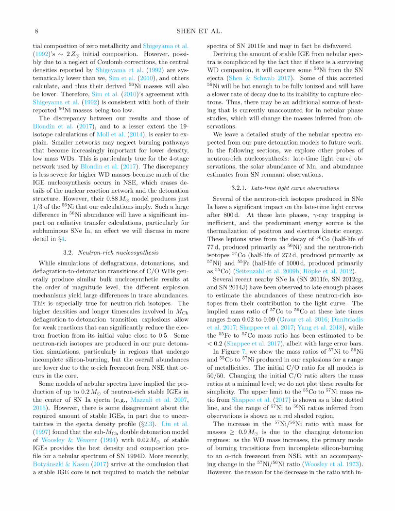
In Figure 7, we show the mass ratios of 57Ni to 56Ni

and 55Co to 57Ni produced in our explosions for a range

of metallicities. The initial C/O ratio for all models is

50/50. Changing the initial C/O ratio alters the mass

ratios at a minimal level; we do not plot these results for

simplicity. The upper limit to the 55Co to 57Ni mass ra-

tio from Shappee et al. (2017) is shown as a blue dotted

line, and the range of 57Ni to 56Ni ratios inferred from

observations is shown as a red shaded region.

The increase in the 57Ni/56Ni ratio with mass for

masses ≥ 0.9M� is due to the changing detonation

regimes: as the WD mass increases, the primary mode

of burning transitions from incomplete silicon-burning

to an α-rich freezeout from NSE, with an accompany-

ing change in the 57Ni/56Ni ratio (Woosley et al. 1973).

However, the reason for the decrease in the ratio with in-

Sub-MCh WD detonations 9

➜

2Z�0Z� 55Co/57Ni mass ratio

57Ni/56Ni mass ratio

2Z�

0Z�

0.8 0.9 1.0 1.1

10−2

10−1

1

MWD/M�

57Ni/

56Nian

d55Co/

57Nimassratios

Figure 7. Mass ratios of 57Ni to 56Ni (red) and 55Co to 57Ni(blue) vs. WD mass from our post-processed nucleosyntheticresults for an initial C/O ratio of 50/50. Four metallicitiesare shown, increasing from bottom to top for each mass ratio:0, 0.5, 1, and 2Z�. The blue dotted line shows an upper limitto the 55Co to 57Ni ratio in SN 2011fe (Shappee et al. 2017),and the red shaded region shows a range of estimated 57Ni to56Ni ratios for SN 2011fe (Dimitriadis et al. 2017; Shappeeet al. 2017), SN 2012cg (Graur et al. 2016), and SN 2014J(Yang et al. 2018).

creasing mass below 0.9M� is uncertain. Similarly, the

origin of the large gap in the 55Co/57Ni ratio between

zero and half solar metallicity models is unknown. This

gap is driven by the metallicity dependence of the 55Co

yield, which is also displayed in Figure 8, but the reason

for this dependence is unclear. We leave exploration of

these trends to future work.

Our 1.1M� results agree broadly with Pakmor et al.

(2012)’s values for a 0.9 + 1.1M� violent merger of two

WDs, whose nucleosynthesis is primarily determined by

the explosion of the more massive WD. Our results for

the range of masses and metallicities do not alter the ten-

sion between the low 57Ni masses produced in sub-MCh

detonation models and the higher masses inferred from

late-time observations. However, the 57Ni and 55Co

masses derived from observations have very large error

bars due to the possible contribution of light echoes and

uncertainties in the γ-ray and lepton trapping efficien-

cies.

Furthermore, the possibility of a surviving compan-

ion WD that complicates nebular spectra modeling will

also have an influence here (Shen & Schwab 2017). If

a companion WD survives the SN Ia explosion, it will

capture a small amount of 56Ni. The radioactive de-

cay of this accreted ejecta will be delayed due to the

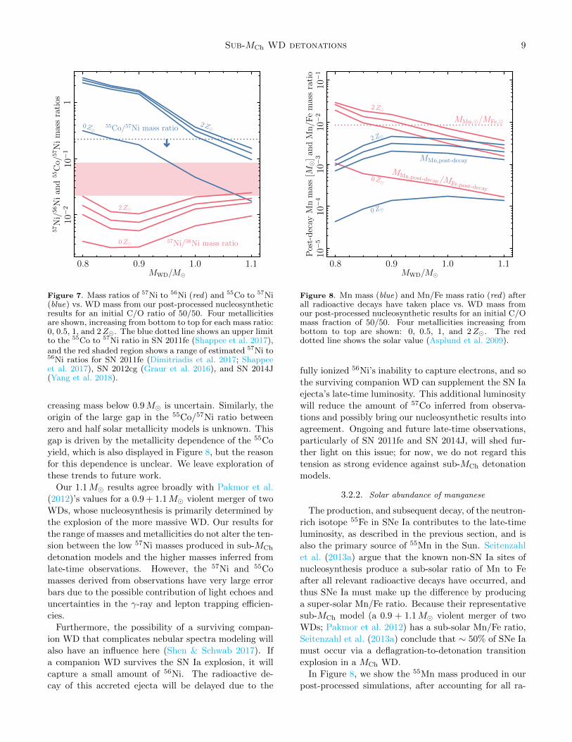
MMn,post-decay

MMn,post-decay/MFe,post-decay

MMn,�/MFe,�

2Z�

0Z�

2Z�

0Z�

0.8 0.9 1.0 1.1

10−5

10−4

10−3

10−2

10−1

MWD/M�

Post-decay

Mnmass[M

�]an

dMn/F

emassratio

Figure 8. Mn mass (blue) and Mn/Fe mass ratio (red) afterall radioactive decays have taken place vs. WD mass fromour post-processed nucleosynthetic results for an initial C/Omass fraction of 50/50. Four metallicities increasing frombottom to top are shown: 0, 0.5, 1, and 2Z�. The reddotted line shows the solar value (Asplund et al. 2009).

fully ionized 56Ni’s inability to capture electrons, and so

the surviving companion WD can supplement the SN Ia

ejecta’s late-time luminosity. This additional luminosity

will reduce the amount of 57Co inferred from observa-

tions and possibly bring our nucleosynthetic results into

agreement. Ongoing and future late-time observations,

particularly of SN 2011fe and SN 2014J, will shed fur-

ther light on this issue; for now, we do not regard this

tension as strong evidence against sub-MCh detonation

models.

3.2.2. Solar abundance of manganese

The production, and subsequent decay, of the neutron-

rich isotope 55Fe in SNe Ia contributes to the late-time

luminosity, as described in the previous section, and is

also the primary source of 55Mn in the Sun. Seitenzahl

et al. (2013a) argue that the known non-SN Ia sites of

nucleosynthesis produce a sub-solar ratio of Mn to Fe

after all relevant radioactive decays have occurred, and

thus SNe Ia must make up the difference by producing

a super-solar Mn/Fe ratio. Because their representative

sub-MCh model (a 0.9 + 1.1M� violent merger of two

WDs; Pakmor et al. 2012) has a sub-solar Mn/Fe ratio,

Seitenzahl et al. (2013a) conclude that ∼ 50% of SNe Ia

must occur via a deflagration-to-detonation transition

explosion in a MCh WD.

In Figure 8, we show the 55Mn mass produced in our

post-processed simulations, after accounting for all ra-

10 SHEN ET AL.

dioactive decays, vs. WD mass for an initial C/O mass

ratio of 50/50. Red lines show the mass ratio of Mn

to Fe, again after all decays have occurred. As before,

changing the initial C/O ratio has a minimal effect on

these results, so these models are omitted for simplicity.

For our lowest mass models, 55Co, which eventually

decays to 55Mn, is produced via incomplete silicon-

burning. As the WD mass and central density are in-

creased, more of the WD core undergoes incomplete

silicon-burning, so the final 55Mn yield increases. How-

ever, the 56Ni yield increases more strongly with WD

mass, so the overall final Mn/Fe ratio decreases. As the

WD mass increases past ∼ 0.9M�, some of the det-

onated material enters the regime of α-rich freezeout

from NSE, which reduces the yield of 55Co (Woosley

et al. 1973; Seitenzahl et al. 2013a) and the Mn/Fe ra-

tio. Presumably, for even higher mass pure detonation

models, the detonated material will reach conditions for

a “normal” freezeout from NSE, and the 55Co yield will

again increase with mass, but our highest mass WD ex-

plosions are not yet in this regime.

The solar value of the Mn/Fe mass ratio is shown as

a red dotted line (Asplund et al. 2009). In agreement

with Pakmor et al. (2012)’s 1.1M� WD detonation, our

higher-mass ≥ 1.0M� models yield sub-solar Mn/Fe

mass ratios. However, a super-solar value is achieved for

lower-mass ≤ 0.9M� detonations at an initial metallic-

ity of 0.5Z�.

Thus, at least part of the discrepancy found by Seiten-

zahl et al. (2013a) between the solar Mn/Fe ratio and nu-

cleosynthesis in sub-MCh detonations can be alleviated

by including pure detonations of lower-mass WDs. How-

ever, unless lower-mass detonations significantly out-

number higher-mass explosions, it is not clear that only

including core collapse SNe and sub-MCh WD detona-

tions will yield the solar Mn/Fe value. The possibility

remains that a combination of core collapse SNe, sub-

MCh WD detonations, and the class of peculiar Type

Iax SNe (Foley et al. 2013; Fink et al. 2014) may yield

the correct solar value, or that MCh explosions do indeed

contribute to Mn production but at a lower fraction of

all SNe Ia; further work is still required to solve this

issue.

3.2.3. SN remnant observations: Mn/Fe vs. Ni/Fe

SN remnants serve as another probe of detailed nu-

cleosynthesis in SN Ia explosions. As the ejecta sweeps

up the surrounding interstellar medium, a reverse shock

propagates into the ejecta, exciting it to X-ray-emitting

temperatures. The resulting emission can be used to in-

fer nucleosynthetic yields, although the process is com-

plicated by noisy spectra, non-equilibrium ionization ef-

fects, asymmetric and inhomogeneous density distribu-

tions, and incomplete propagation of the reverse shock

▲

■★

●

■

▲

■

★

●

■

▲

■★

●

■

▲

■★

●

■

▲

■

★

●

■

3C 397

Tycho

Kepler

0.8M�0.85M�0.9M�1.0M�1.1M�

0Z�

0.5Z�

1Z�

2Z�

10−4 10−3 10−2 10−1

10−3

10−2

10−1

MNi/MFe in SN remnant

MMn/M

Fein

SN

remnan

t

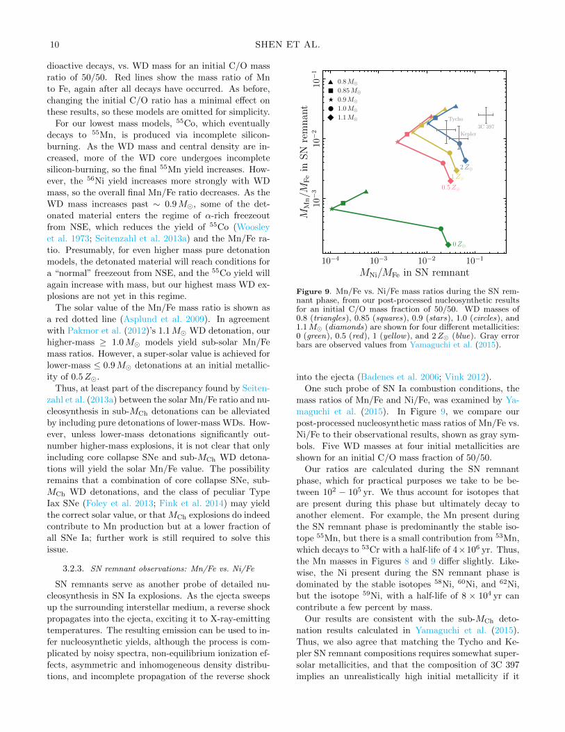
Figure 9. Mn/Fe vs. Ni/Fe mass ratios during the SN rem-nant phase, from our post-processed nucleosynthetic resultsfor an initial C/O mass fraction of 50/50. WD masses of0.8 (triangles), 0.85 (squares), 0.9 (stars), 1.0 (circles), and1.1M� (diamonds) are shown for four different metallicities:0 (green), 0.5 (red), 1 (yellow), and 2Z� (blue). Gray errorbars are observed values from Yamaguchi et al. (2015).

into the ejecta (Badenes et al. 2006; Vink 2012).

One such probe of SN Ia combustion conditions, the

mass ratios of Mn/Fe and Ni/Fe, was examined by Ya-

maguchi et al. (2015). In Figure 9, we compare our

post-processed nucleosynthetic mass ratios of Mn/Fe vs.

Ni/Fe to their observational results, shown as gray sym-

bols. Five WD masses at four initial metallicities are

shown for an initial C/O mass fraction of 50/50.

Our ratios are calculated during the SN remnant

phase, which for practical purposes we take to be be-

tween 102 − 105 yr. We thus account for isotopes that

are present during this phase but ultimately decay to

another element. For example, the Mn present during

the SN remnant phase is predominantly the stable iso-

tope 55Mn, but there is a small contribution from 53Mn,

which decays to 53Cr with a half-life of 4×106 yr. Thus,

the Mn masses in Figures 8 and 9 differ slightly. Like-

wise, the Ni present during the SN remnant phase is

dominated by the stable isotopes 58Ni, 60Ni, and 62Ni,

but the isotope 59Ni, with a half-life of 8 × 104 yr can

contribute a few percent by mass.

Our results are consistent with the sub-MCh deto-

nation results calculated in Yamaguchi et al. (2015).

Thus, we also agree that matching the Tycho and Ke-

pler SN remnant compositions requires somewhat super-

solar metallicities, and that the composition of 3C 397

implies an unrealistically high initial metallicity if it

Sub-MCh WD detonations 11

▲

■

★

●

▲

■

★●

▲

■

★●

▲

■

★●

▲

■

★

●

100% reverse-shocked

75% reverse-shocked

50% reverse-shocked

25% reverse-shocked

0Z�

0.5Z�

1Z�

2Z�

M = 0.9M�

3C 397

Tycho

Kepler

10−4 10−3 10−2 10−1

10−3

10−2

10−1

MNi/MFe in SN remnant

MMn/M

Fein

SN

remnan

t

Figure 10. Mn/Fe mass ratio vs. Ni/Fe mass ratio forour 0.9M� models with varying metallicities and varyingamounts of reverse-shocked ejecta. Green, red, yellow, andblue curves represent models with initial metallicities of 0,0.5, 1.0, and 2.0Z�, respectively. The fraction of the ejectathat has been reverse-shocked decreases from 100% on theleft (triangles) to 25% on the right (circles).

was the product of a sub-MCh explosion. Yamaguchi

et al. (2015) claim that this mismatch is evidence for a

MCh explosion, but we emphasize that a MCh explana-

tion also requires an extremely high metallicity, a com-

plicated ejecta geometry, an unexpectedly high central

density (Dave et al. 2017), or a combination of all three.

Thus, the abundances in SN remnant 3C 397 continue

to present a nucleosynthetic puzzle for any standard sce-

nario.

The implication that Tycho and Kepler’s exploding

WDs had super-solar metallicities is also somewhat

problematic, given the solar or slightly sub-solar metal-

licities of the stellar environments at their Galactocen-

tric radii (Martınez-Rodrıguez et al. 2017). However,

this discrepancy can be at least partially explained by

the fact that these remnants are young and their reverse

shocks have not fully traversed the SN ejecta. Thus, the

inferred mass ratios may not be representative of the

ejecta’s total nucleosynthesis.

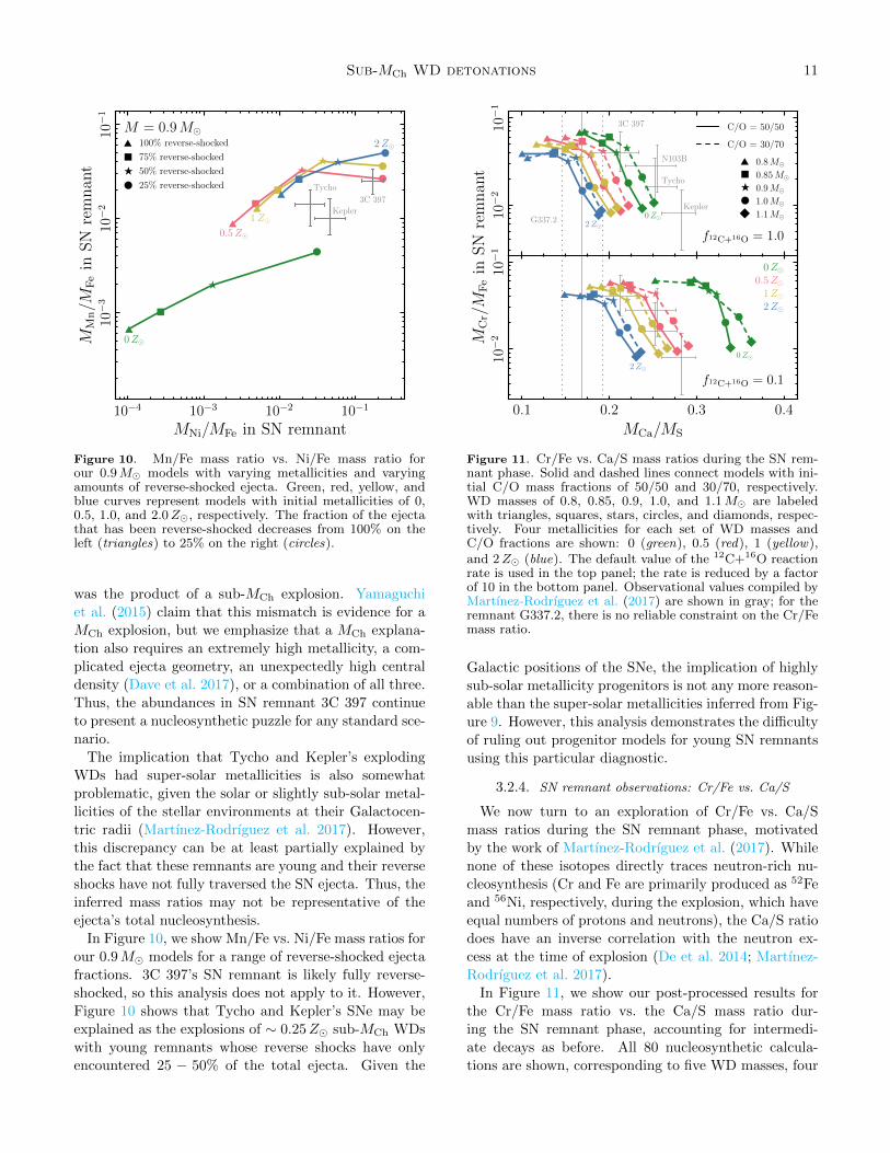
In Figure 10, we show Mn/Fe vs. Ni/Fe mass ratios for

our 0.9M� models for a range of reverse-shocked ejecta

fractions. 3C 397’s SN remnant is likely fully reverse-

shocked, so this analysis does not apply to it. However,

Figure 10 shows that Tycho and Kepler’s SNe may be

explained as the explosions of ∼ 0.25Z� sub-MCh WDs

with young remnants whose reverse shocks have only

encountered 25 − 50% of the total ejecta. Given the

▲■

★

●

■

▲■

★

●

■

▲■

★

●

■

▲ ■★

●

■

▲■

★

●

■

▲ ■★

●

■

▲ ■★

●

■

▲■

★

●

■

▲

■

★

●

■

▲■

★

●

■

▲■

★

●

■

▲■

★

●

■

▲ ■★

●

■

▲ ■★

●

■

▲■★

●

■

▲ ■★

●

■

▲ ■★

●

■

G337.2

3C 397

N103B

Tycho

Kepler

C/O = 50/50

C/O = 30/70

0.8M�0.85M�0.9M�1.0M�1.1M�

f12C+16O = 1.0

0Z�2Z�

10−2

10−1

f12C+16O = 0.1

0Z�0.5Z�1Z�2Z�

0Z�2Z�

0.1 0.2 0.3 0.4

10−2

10−1

MCa/MS

MCr/M

Fein

SN

remnan

t

Figure 11. Cr/Fe vs. Ca/S mass ratios during the SN rem-nant phase. Solid and dashed lines connect models with ini-tial C/O mass fractions of 50/50 and 30/70, respectively.WD masses of 0.8, 0.85, 0.9, 1.0, and 1.1M� are labeledwith triangles, squares, stars, circles, and diamonds, respec-tively. Four metallicities for each set of WD masses andC/O fractions are shown: 0 (green), 0.5 (red), 1 (yellow),and 2Z� (blue). The default value of the 12C+16O reactionrate is used in the top panel; the rate is reduced by a factorof 10 in the bottom panel. Observational values compiled byMartınez-Rodrıguez et al. (2017) are shown in gray; for theremnant G337.2, there is no reliable constraint on the Cr/Femass ratio.

Galactic positions of the SNe, the implication of highly

sub-solar metallicity progenitors is not any more reason-

able than the super-solar metallicities inferred from Fig-

ure 9. However, this analysis demonstrates the difficulty

of ruling out progenitor models for young SN remnantsusing this particular diagnostic.

3.2.4. SN remnant observations: Cr/Fe vs. Ca/S

We now turn to an exploration of Cr/Fe vs. Ca/S

mass ratios during the SN remnant phase, motivated

by the work of Martınez-Rodrıguez et al. (2017). While

none of these isotopes directly traces neutron-rich nu-

cleosynthesis (Cr and Fe are primarily produced as 52Fe

and 56Ni, respectively, during the explosion, which have

equal numbers of protons and neutrons), the Ca/S ratio

does have an inverse correlation with the neutron ex-

cess at the time of explosion (De et al. 2014; Martınez-

Rodrıguez et al. 2017).

In Figure 11, we show our post-processed results for

the Cr/Fe mass ratio vs. the Ca/S mass ratio dur-

ing the SN remnant phase, accounting for intermedi-

ate decays as before. All 80 nucleosynthetic calcula-

tions are shown, corresponding to five WD masses, four

12 SHEN ET AL.

metallicities, initial C/O mass fractions of 50/50 and

30/70, and two choices for the 12C+16O reaction rate:

the default REACLIB reaction rate (Caughlan & Fowler

1988) and the rate scaled by a multiplicative factor,

f12C+16O = 0.1, as motivated by Martınez-Rodrıguez

et al. (2017). Observational values for five Galactic and

LMC remnants from Martınez-Rodrıguez et al. (2017)

are shown in gray. The remnant G337.2 does not have

constraints on its Cr/Fe mass ratio, so it is shown as a

vertical band.

It is clear that only very low metallicity 30/70 C/O

explosions in the top panel are consistent with the ob-

served SN remnants. As previously mentioned, there is

some uncertainty in the fact that some of these rem-

nants may not be old enough to have their entire ejecta

traversed by the reverse shock, so that the mass ratios

inferred from observations may not be representative of

the entire ejecta. However, the primary discrepancy lies

in the Ca/S ratio, and since these IMEs are located in

the outer parts of the ejecta, they have likely already

been excited by the reverse shock.

Much better agreement is found in the bottom panel,

for which the 12C+16O reaction rate is reduced by a

factor of 10. Here, solar and sub-solar metallicities

and C/O ratios of both 50/50 and 30/70 match val-

ues for observed SN remnants. Our results are consis-

tent with Martınez-Rodrıguez et al. (2017)’s findings; as

they explain, a slower 12C+16O reaction rate increases

the abundance of 4He nuclei, which favors the produc-

tion of isotopes higher in the α-chain, and thus a higher

Ca/S ratio.

However, the 12C+16O is not actually uncertain to a

factor of 10. Unlike for the typical relatively low-energy

stellar case, reaction rates at energies relevant to stel-

lar detonations can be probed in the laboratory. The

burning temperature ∼ 4 × 109 K of the carbon det-

onation yields a Gamow peak of 7.7 MeV with width

3.8 MeV, an energy range at which the cross-section of

the 12C+16O reaction has been directly measured. The

S factor at the Gamow peak has an experimental uncer-

tainty of only ∼ 50%, and its median is actually ∼ 20%

higher than the Caughlan & Fowler (1988) value used in

REACLIB (Patterson et al. 1971; Cujec & Barnes 1976;

Christensen et al. 1977; Jiang et al. 2007). The un-

certainty at lower energies within the peak is higher, a

factor of ∼ 2, but since the rate is dominated by the

cross-section near the peak’s maximum, the rate is only

uncertain by ∼ 50% at our temperatures of interest.

Thus, while we do find good agreement with the ob-

served Ca/S ratio in the Tycho and Kepler SN remnants

for near-solar metallicities and a reduced 12C+16O re-

action rate, this is not a likely explanation. Using the

default REACLIB Caughlan & Fowler (1988) rate, our

sub-MCh models imply low metallicity progenitors for

these remnants. However, we note that the MCh mod-

els in Martınez-Rodrıguez et al. (2017) yield a similar

conclusion when the default 12C+16O reaction rate is

used.

4. RADIATIVE TRANSFER CALCULATIONS

A stringent test of the validity of our sub-MCh WD

detonation models is a comparison to the rich SN Ia ob-

servational data sets collected in the past few decades.

To this end, we employ the Monte Carlo radiative trans-

fer code SEDONA (Kasen et al. 2006) to produce syn-

thetic light curves and spectra, which we discuss and

compare to observations in the following sections. These

calculations assume the level populations are in local

thermodynamic equilibrium (LTE) and that lines are

purely absorbing. Note that we only consider compar-

isons to “normal” SNe Ia, ranging from SN 1991bg-likes

to SN 1991T-likes, and not to the peculiar classes of Ca-

rich transients (e.g., Kasliwal et al. 2012) and SNe Iax

(e.g., Foley et al. 2013).

4.1. Light curves

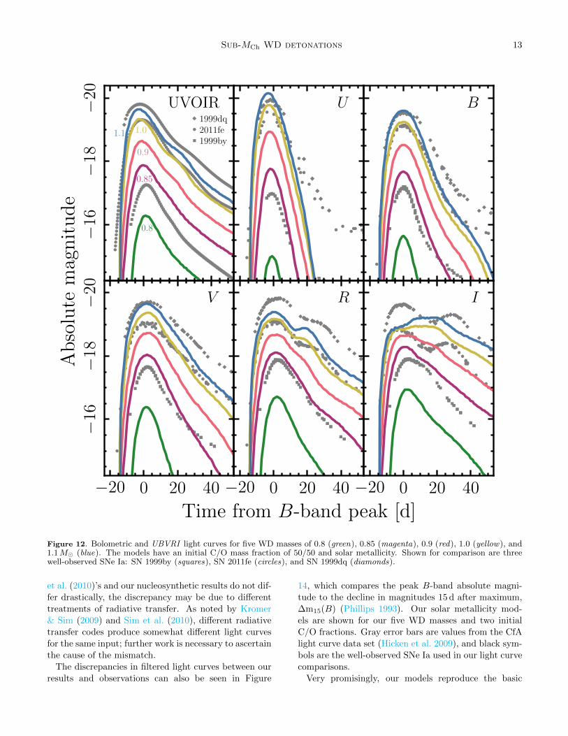
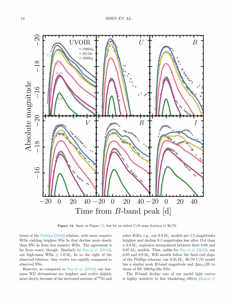
Figures 12 and 13 show bolometric and broad-band

light curves for post-processed models with solar metal-

licity and initial C/O mass fractions of 50/50 and 30/70,

respectively. Vega magnitudes are used here and in the

following. Also overlaid for comparison in gray are three

well-observed SNe Ia: the subluminous 1991bg-like SN

1999by (Garnavich et al. 2004; Stritzinger 2005; Gane-

shalingam et al. 2010), the normal SN 2011fe (Munari

et al. 2013; Pereira et al. 2013; Tsvetkov et al. 2013), and

the over-luminous 1991T-like SN 1999dq (Stritzinger

2005; Jha et al. 2006; Ganeshalingam et al. 2010).3

The general shapes of our synthetic bolometric light

curves show good agreement with observed SNe Ia. Thesubluminous SN 1999by is reasonably well fit by our

0.85M� 30/70 C/O model, the normal SN 2011fe agrees

with the 1.0M� models, and the over-luminous SN

1999dq is somewhat brighter than our 1.1M� models.

However, there are some discrepancies in the filtered

light curves. In particular, our synthetic light curves

generally fall too rapidly in the U and B bands and

remain too bright in the R and I bands.

Our results are in broad agreement with those of Sim

et al. (2010), although our different nucleosynthetic out-

put precludes an exact comparison. One notable differ-

ence is obvious after 30 d, when our bluer light curves de-

viate from observations, whereas Sim et al. (2010)’s flat-

ten and provide a better match to observations. Since

this difference persists for higher WD masses, where Sim

3 Much of the data used in this work was obtained throughhttps://sne.space (Guillochon et al. 2017).

Sub-MCh WD detonations 13

■

■■■■■

■■■■■■■■■■■■■■■■■■

■■■■■■■■■■■■■■■■■■■■■■■■■■■■■■■■■■■■■■■■■■■■■■■■■■■■■■■■■■■■■■■■■■■■■■■■■■■■■■■■■■■■■■■■■■■■■■■■■■■■■■■■■■■■■■■■■■■■■■■■■■■■■■■■■■■■■■■■■■■■■■■■■■■■■■■■■■■■■■■■■■■■■■■■■■■■■■■

●●●●●●●●●●●●●●●●●●●●●●●●●●●●●●●●●●●●●●●

●●●●●●●●●●●●●●●●●●●●●●●●●●●●●●●●●●●●●●●●●●●●●●●●●●●●●●●●●●●●●●●●●●●●●●●●●●●●●●●●●●●●●●●●●●●●●●●●●●●●●●●●●●●●●●●●●●●●●●●●●

■

■■■■■■■■■■■■■■■■■■■■■■■■■

■■■■■■■■■■■■■■■■■■■■■■■■■■■■■■■■■■■■■■■■■■■■■■■■■■■■■■■■■■■■■■■■■■■■■■■■■■■■■■■■■■■■■■■■■■■■■■■■■■■■■■■■■■■■■■■■■■■■■■■■■■■■■■■■■■■■■■■■■■■■■■■■■■■■■■■■■■■■■■■■■■■■■■■■■■■■■

■

●

■

■■

■■

■■■■■■■■■■■■■■

■■■■■■■■

■■

■■

■■

■■

■■

■■

■■

■■

■■

●

●

●

●

●

●●

●●

●●

●●

●●●

●●●

●●

●●●●

●

●

●

●

●

●

●

●

●●

●●● ●

● ●●

●

●

●

●● ●

●

●

●

●●

●

●

●

●

●

●

■■■■■■■■■■■■

■■■■

■■

■■

■■

■■

■■

■■

■■■■■■

■■ ■■■■

■■

■

■

■■■

■■■■■■■■■■■■■■■■■■■■■■■■■■■■■■■■■ ■■ ■

■

■

■■■

■

■■■■

■■■

■■■

■

■■■

■■■ ■■

■■

■■

■■

■■

■■

■■

■■

●

●

●

●●

●●

●●●●

●●●

●

●●●●●●●●●●●●●

●●●●●●●●

●●●●●●

●●●●●●●●●●●●●●●●●●●●●●●●

●●●●●●

●●●●●● ●

●● ● ●● ●●●●●●●●●●●●●●●●●●●●●●●

●●●●● ●●●●●●●●●●●●

●●

●● ●● ●●●●●●●

●●●●

●●●● ●●●

●●●●●●●●●●●● ● ●

●●●●●●●●●●●●●

●●●●●●●●●●●

●●●●●● ●●

●●●

●●●●●●

●●●●●●

●●

●●●

●

● ●●

● ●●

●●● ●

● ●●●

●●

●●

■

■■■■■■■■■■■■■■■■■■■■■■■■■■■■■■■

■■■

■■■

■■■

■

■■■

■■

■■■

■■■

■■■■

■■■■■■

■■■■

■■

■■

■

■

■■■■■■■■■■■■■■■■■■■■■■■■■■■

■■■■■■■■■ ■■ ■■

■■■■■■■

■■■■■■■

■■■■■■■■■■

■■

■■

■■

■■■■

■■

■■■■

■■■■

●

●

●

●●

●

●

●●●

●

●●

●●

●●

●●●●●●

●●●●●●●●

●●●●●

●●●●●●●●●●●●●●●●●●●●●●●●●

●●●●●

●●●●●

●●

●●●●●

●●

●●

●●●●●●●●●

●●●●●●●●●●●●●●●

●

●●●●●

●●●●●●●●●●●

●●

●

●●●

●●●●●●

●●●●●●●●

●●●

●●●●●●●●●●●●

●●● ● ●●●●●●●●●●

●

●●● ●●●●●●●●●●●●●●●●●

●● ●●

●●●●●●

●●●●●●● ●

●●●●●

● ●●●

●

●● ●

●

●● ●

●●●●

●

●●

●

■

■

■■■■■■■■■■■■■■■■■■

■■■■■■■■■■■■■■■■■■■■■■■■■■■

■■■

■■■

■■■■

■■■■■

■■

■■■■

■■

■■

■

■

■■■

■■■■■■■■■■■■■■■■■■■■■■■■

■■■■■■■■■■■ ■■■

■

■ ■■■■■■ ■■■■ ■■■ ■■■ ■■■■■■■

■■

■■

■■

■■

■■

■■

■■

■■

■■

●

●

●

●●

●●

●●●

●●●●

●●●●●●●●●●●

●●●●●●

●●●●●

●●●●●●

●●●●●●●●●●●●●●●●●●●●●●●

●●●●●

●●

●●●●●

●

●●

●●●

●●●●●●●●●●●●

●●●●●●●●●●

●

●●●

●● ●●●●

●●●●●●●●

●●●

●● ●●

●●●●●●●●●●●

●●●●

●●●●●●●●●●●●●●●● ●

●●●●●●●●●●

●●● ●

●●●●●●●●●

●●●●●●●

●● ●●

●

●

●●●●

●●

●

●

●●●

●●●●

●●●●

●

●

●●

●

●●●

●●● ●

●●●

■

■■■■■■■■■■■■■■■■■■■■■■■■■■■■■■■■■■

■■■■■■■

■■■■■

■■■

■■■

■■■■■■■

■■■■

■■■■

■■

■■

■

■

■■■■■■■■■■■■■■■■■■■■■■■■■■■■■■■■■■■ ■■

■

■ ■■■■■■

■■■ ■■■ ■■■ ■■■■■■■■

■

■

■

■■

■■

■■■■

■■

■■■■

●

●

●

●●

●●●

●●●

●●●●

●●●●●●

●●●●●●●●●●●●●

●●●●●●

●●●●●●●●●

●●●●●●●●●●●●

●● ●●●●●

●●

●●●●●

●

●●

●

●●

●●●●●●●●

●●●●●●●●●

●●●●●

●

●●●●

●●●●●

●●●●●●●●●

●●

●● ●●

●●●●●●●●●●●

● ●●●●●●●●●

●●●●●●●●● ● ●

●●●●●●●●●●

●●●

●●●

●●●

●●●●●●●●●●

● ●● ●●

●●●●●●●

●●

●●●● ●

● ●●

●●

●●

●●

●

●●●

●●

●●●

●●

●

●

■

■■■■■■■■■■■■■■■■■■■■■■■■■■■■■■■■■■■■■■■■■

■■■■■■■

■

■■■

■■■■

■■■■■

■■

■■■■

■■

■■

UVOIR

1.1 1.0

0.9

0.85

0.8

1999dq2011fe1999by

−20

−18

−16

U B

V

−20 0 20 40

−20

−18

−16

Absolute

magnitude

R

−20 0 20 40

Time from B-band peak [d]

I

−20 0 20 40

Figure 12. Bolometric and UBVRI light curves for five WD masses of 0.8 (green), 0.85 (magenta), 0.9 (red), 1.0 (yellow), and1.1M� (blue). The models have an initial C/O mass fraction of 50/50 and solar metallicity. Shown for comparison are threewell-observed SNe Ia: SN 1999by (squares), SN 2011fe (circles), and SN 1999dq (diamonds).

et al. (2010)’s and our nucleosynthetic results do not dif-

fer drastically, the discrepancy may be due to different

treatments of radiative transfer. As noted by Kromer

& Sim (2009) and Sim et al. (2010), different radiative

transfer codes produce somewhat different light curves

for the same input; further work is necessary to ascertain

the cause of the mismatch.

The discrepancies in filtered light curves between our

results and observations can also be seen in Figure

14, which compares the peak B-band absolute magni-

tude to the decline in magnitudes 15 d after maximum,

∆m15(B) (Phillips 1993). Our solar metallicity mod-

els are shown for our five WD masses and two initial

C/O fractions. Gray error bars are values from the CfA

light curve data set (Hicken et al. 2009), and black sym-

bols are the well-observed SNe Ia used in our light curve

comparisons.

Very promisingly, our models reproduce the basic

14 SHEN ET AL.

■

■■■■■

■■■■■■■■■■■■■■■■■■

■■■■■■■■■■■■■■■■■■■■■■■■■■■■■■■■■■■■■■■■■■■■■■■■■■■■■■■■■■■■■■■■■■■■■■■■■■■■■■■■■■■■■■■■■■■■■■■■■■■■■■■■■■■■■■■■■■■■■■■■■■■■■■■■■■■■■■■■■■■■■■■■■■■■■■■■■■■■■■■■■■■■■■■■■■■■■■■

●●●●●●●●●●●●●●●●●●●●●●●●●●●●●●●●●●●●●●●

●●●●●●●●●●●●●●●●●●●●●●●●●●●●●●●●●●●●●●●●●●●●●●●●●●●●●●●●●●●●●●●●●●●●●●●●●●●●●●●●●●●●●●●●●●●●●●●●●●●●●●●●●●●●●●●●●●●●●●●●●

■

■■■■■■■■■■■■■■■■■■■■■■■■■

■■■■■■■■■■■■■■■■■■■■■■■■■■■■■■■■■■■■■■■■■■■■■■■■■■■■■■■■■■■■■■■■■■■■■■■■■■■■■■■■■■■■■■■■■■■■■■■■■■■■■■■■■■■■■■■■■■■■■■■■■■■■■■■■■■■■■■■■■■■■■■■■■■■■■■■■■■■■■■■■■■■■■■■■■■■■■

■

●

■

■■

■■

■■■■■■■■■■■■■■

■■■■■■■■

■■

■■

■■

■■

■■

■■

■■

■■

■■

●

●

●

●

●

●●

●●

●●

●●

●●●

●●●

●●

●●●●

●

●

●

●

●

●

●

●

●●

●●● ●

● ●●

●

●

●

●● ●

●

●

●

●●

●

●

●

●

●

●

■■■■■■■■■■■■

■■■■

■■

■■

■■

■■

■■

■■

■■■■■■

■■ ■■■■

■■

■

■

■■■

■■■■■■■■■■■■■■■■■■■■■■■■■■■■■■■■■ ■■ ■

■

■

■■■

■

■■■■

■■■

■■■

■

■■■

■■■ ■■

■■

■■

■■

■■

■■

■■

■■

●

●

●

●●

●●

●●●●

●●●

●

●●●●●●●●●●●●●

●●●●●●●●

●●●●●●

●●●●●●●●●●●●●●●●●●●●●●●●

●●●●●●

●●●●●● ●

●● ● ●● ●●●●●●●●●●●●●●●●●●●●●●●

●●●●● ●●●●●●●●●●●●

●●

●● ●● ●●●●●●●

●●●●

●●●● ●●●

●●●●●●●●●●●● ● ●

●●●●●●●●●●●●●

●●●●●●●●●●●

●●●●●● ●●

●●●

●●●●●●

●●●●●●

●●

●●●

●

● ●●

● ●●

●●● ●

● ●●●

●●

●●

■

■■■■■■■■■■■■■■■■■■■■■■■■■■■■■■■

■■■

■■■

■■■

■

■■■

■■

■■■

■■■

■■■■

■■■■■■

■■■■

■■

■■

■

■

■■■■■■■■■■■■■■■■■■■■■■■■■■■

■■■■■■■■■ ■■ ■■

■■■■■■■

■■■■■■■

■■■■■■■■■■

■■

■■

■■

■■■■

■■

■■■■

■■■■

●

●

●

●●

●

●

●●●

●

●●

●●

●●

●●●●●●

●●●●●●●●

●●●●●

●●●●●●●●●●●●●●●●●●●●●●●●●

●●●●●

●●●●●

●●

●●●●●

●●

●●

●●●●●●●●●

●●●●●●●●●●●●●●●

●

●●●●●

●●●●●●●●●●●

●●

●

●●●

●●●●●●

●●●●●●●●

●●●

●●●●●●●●●●●●

●●● ● ●●●●●●●●●●

●

●●● ●●●●●●●●●●●●●●●●●

●● ●●

●●●●●●

●●●●●●● ●

●●●●●

● ●●●

●

●● ●

●

●● ●

●●●●

●

●●

●

■

■

■■■■■■■■■■■■■■■■■■

■■■■■■■■■■■■■■■■■■■■■■■■■■■

■■■

■■■

■■■■

■■■■■

■■

■■■■

■■

■■

■

■

■■■

■■■■■■■■■■■■■■■■■■■■■■■■

■■■■■■■■■■■ ■■■

■

■ ■■■■■■ ■■■■ ■■■ ■■■ ■■■■■■■

■■

■■

■■

■■

■■

■■

■■

■■

■■

●

●

●

●●

●●

●●●

●●●●

●●●●●●●●●●●

●●●●●●

●●●●●

●●●●●●

●●●●●●●●●●●●●●●●●●●●●●●

●●●●●

●●

●●●●●

●

●●

●●●

●●●●●●●●●●●●

●●●●●●●●●●

●

●●●

●● ●●●●

●●●●●●●●

●●●

●● ●●

●●●●●●●●●●●

●●●●

●●●●●●●●●●●●●●●● ●

●●●●●●●●●●

●●● ●

●●●●●●●●●

●●●●●●●

●● ●●

●

●

●●●●

●●

●

●

●●●

●●●●

●●●●

●

●

●●

●

●●●

●●● ●

●●●

■

■■■■■■■■■■■■■■■■■■■■■■■■■■■■■■■■■■

■■■■■■■

■■■■■

■■■

■■■

■■■■■■■

■■■■

■■■■

■■

■■

■

■

■■■■■■■■■■■■■■■■■■■■■■■■■■■■■■■■■■■ ■■

■

■ ■■■■■■

■■■ ■■■ ■■■ ■■■■■■■■

■

■

■

■■

■■

■■■■

■■

■■■■

●

●

●

●●

●●●

●●●

●●●●

●●●●●●

●●●●●●●●●●●●●

●●●●●●

●●●●●●●●●

●●●●●●●●●●●●

●● ●●●●●

●●

●●●●●

●

●●

●

●●

●●●●●●●●

●●●●●●●●●

●●●●●

●

●●●●

●●●●●

●●●●●●●●●

●●

●● ●●

●●●●●●●●●●●

● ●●●●●●●●●

●●●●●●●●● ● ●

●●●●●●●●●●

●●●

●●●

●●●

●●●●●●●●●●

● ●● ●●

●●●●●●●

●●

●●●● ●

● ●●

●●

●●

●●

●

●●●

●●

●●●

●●

●

●

■

■■■■■■■■■■■■■■■■■■■■■■■■■■■■■■■■■■■■■■■■■

■■■■■■■

■

■■■

■■■■

■■■■■

■■

■■■■

■■

■■

UVOIR

1.1 1.0

0.9

0.85

0.8

1999dq2011fe1999by

−20

−18

−16

U B

V

−20 0 20 40

−20

−18

−16

Absolute

magnitude

R

−20 0 20 40

Time from B-band peak [d]

I

−20 0 20 40

Figure 13. Same as Figure 12, but for an initial C/O mass fraction of 30/70.

trend of the Phillips (1993) relation, with more massive

WDs yielding brighter SNe Ia that decline more slowly

than SNe Ia from less massive WDs. The agreement is

far from exact, though. Similarly to Sim et al. (2010),

our high-mass WDs ≥ 1.0M� lie to the right of the

observed relation: they evolve too rapidly compared to

observed SNe.

However, as compared to Sim et al. (2010), our low-

mass WD detonations are brighter and evolve slightly

more slowly because of the increased amount of 56Ni and

other IGEs; e.g., our 0.9M� models are 1.5 magnitudes

brighter and decline 0.1 magnitudes less after 15 d than

a 0.9M� explosion interpolated between their 0.88 and

0.97M� models. Thus, unlike for Sim et al. (2010), our

0.85 and 0.9M� WD models follow the faint-end slope

of the Phillips relation; our 0.85M� 30/70 C/O model

has a similar peak B-band magnitude and ∆m15(B) to

those of SN 1991bg-like SNe.

The B-band decline rate of our model light curvesis highly sensitive to line blanketing effects (Kasen &

Sub-MCh WD detonations 15

●▲

●

▲

●

▲

●▲

●▲

●

▲ 0.8

0.85

0.9

1.0

1.1

C/O= 50/50

C/O= 30/70

1999dq

2011fe

1999by

0.5 1.0 1.5 2.0 2.5 3.0

−20

−19

−18

−17

−16

∆m15(B)

Pea

kB

-ban

dab

solu

tem

agn

itu

de

Figure 14. Peak B-band absolute magnitude vs. ∆m15(B).Green, magenta, red, yellow, and blue triangles and circlesare results from solar metallicity post-processed models, aslabeled. Gray symbols are values taken from the CfA lightcurve data set (Hicken et al. 2009), and black error bars arevalues for SN 1999by, SN 2011fe, and SN 1999dq.

Woosley 2007). The fact that our 1.0 and 1.1M� mod-

els predict too rapid a decline could be related to limi-

tations in the transport calculations. In particular, the

LTE assumption adopted here, which only approximates

the more complex redistribution of photons to longer

wavelengths due to fluorescence, may overestimate the

rate of light curve reddening. As mentioned above, Sim

et al. (2010)’s U - and B-band light curves show some

late-time flattening, which ours do not. This difference

may be related to their use of a method intended to

mimic non-LTE effects.

The importance of these effects is supported by

Blondin et al. (2017)’s non-LTE radiative transfer cal-

culations. The light curves of their ≥ 1.0M� models

decline more slowly than ours and those of Sim et al.

(2010), and they are able to much more closely match

the bright end of the Phillips relation. As discussed in

§3.1.2, the 56Ni yields do not differ significantly among

the various studies at these relatively high masses, and

thus the differences in the light curves of the high mass

explosions may be attributed to their inclusion of non-

LTE effects.

At the low-mass end, Blondin et al. (2017)’s non-

LTE radiative transfer calculations do not reproduce the

Phillips relation, instead yielding light curves that are

too dim. However, our 56Ni yields are several times

higher than theirs in this regime. It is thus possible that

a combination of the nucleosynthesis from our large net-

1999dq+2 d

2011fe

+0 d

1999by−2 d

0.8−2 d

0.85−2 d

0.9−1 d

1.0+1 d

1.1+2 d

2000 3000 4000 5000 6000 7000 8000 9000 10000

01

23

45

6

Wavelength [A]

log10

(Fλ)

+co

nst

ant

Figure 15. Synthetic and observed spectra near maximumB-band magnitude, offset by arbitrary constants. Green,magenta, red, yellow, and blue lines represent solar metallic-ity, 50/50 C/O WDs with masses of 0.8, 0.85, 0.9, 1.0, and1.1M� at −2, −2, −1, +1, and +2 d from B-band maxi-mum, respectively. Observed spectra for SN 1999by at −2 d,SN 2011fe at +0 d, and SN 1999dq at +2 d are shown in gray.Vertical lines are located in the Si ii λ6355 and Ca ii H&Kand near-IR triplet regions to help guide the eye.

work, broadened detonation simulations and non-LTE

radiation transport calculations will reproduce the en-

tirety of the Phillips relation; such a study is currently

underway.

We note that our 0.8M� models do not appear to

match any observed SNe Ia. As argued by Shen & Bild-

sten (2014), this may be due to a physical minimum

WD mass and associated central density that can be

ignited via a converging shock: WDs that are too low

in mass cannot explode as double detonation SNe Ia.

Given the qualitative agreement between our 0.85M�models and SN 1991bg-like SNe, the minimum detonat-

able WD mass may be ' 0.85M�.

4.2. Spectra

Figures 15 and 16 compare synthetic near-maximum

spectra of our five solar metallicity WD models with ini-

tial C/O mass fractions of 50/50 and 30/70, respectively,

to spectra of SN 1999by, SN 2011fe, and SN1999dq at

−2, +0, and +2 d from B-band maximum. While de-

tailed features are not matched precisely, the overall

agreement is promising. Our synthetic spectra show the

hallmark attributes of SNe Ia – strong Si, S, Ca, and Fe

features – with reasonable correspondence to observed

line strengths. The 4000−4500 A Ti ii trough character-

istic of subluminous SNe Ia is also partially reproduced

16 SHEN ET AL.

1999dq+2 d

2011fe

+0 d

1999by−2 d0.8

−2 d

0.85−2 d

0.9−1 d

1.0+1 d

1.1+2 d

2000 3000 4000 5000 6000 7000 8000 9000 10000

01

23

45

6

Wavelength [A]

log10

(Fλ)

+co

nst

ant

Figure 16. Same as Figure 15, but for an initial C/O massfraction of 30/70.

in our least massive 0.8 and 0.85M� models.

One of the most significant discrepancies between our

synthetic spectra and observations are the IME veloci-

ties, particularly for the more massive WDs ≥ 1.0M�and brighter observed SNe. At B-band maximum, the

Si and Ca velocities of our 1.0 and 1.1M� explosions

are several thousand km s−1 higher than observed. It

is possible that non-LTE calculations will alleviate this

discrepancy, as Blondin et al. (2017)’s sub-MCh spectra

possess appropriate line velocities.

A resolution to this issue may also lie in future multi-

dimensional explosion studies of the double detonation

scenario. In the converging shock variant of the double

detonation, a helium shell detonation propagates around

the WD’s surface and launches an oblique shock into the

core that focuses its energy near the center and ignites

the carbon detonation (Livne 1990; Fink et al. 2007,

2010; Shen & Bildsten 2014). This inwardly propagating

shock may tamp the outgoing core detonation somewhat

and reduce the velocities of the outermost ejecta where

the IME features form.

In the edge-lit double detonation variation, the helium

shell detonation transitions into a carbon-powered det-

onation as soon as it encounters the WD core (Taam

1980a,b; Nomoto 1982a; Woosley et al. 1986). Thus,

for one hemisphere of the WD, the carbon detonation

actually moves inwards initially, so that when pressure

forces cause the ejecta to rebound outwards, the outer-

most ejecta velocity will be similarly limited. For the

opposite hemisphere, tamping of the outer ejecta may

still occur if the helium shell detonation races ahead and

reaches the opposite pole before the carbon detonation

traverses the WD core.

Kromer et al. (2010) performed multi-dimensional

converging shock double detonation simulations that are

similar to our planned future calculations. They found

that standard SN Ia light curves and spectra are only

produced if the helium shells are heavily polluted by12C (∼ 30% by mass). However, the minimum deto-

natable helium shell masses found by Shen & Moore

(2014) are an order of magnitude smaller than those

used by Kromer et al. (2010). We remain hopeful that

these much smaller realistic helium shells will still lead to

tamping of the bulk ejecta’s velocities without adversely

affecting the light curves and overall spectra. There is

also the intriguing possibility that these minimal helium

shells, which only produce Si and Ca ashes (Moore et al.

2013; Shen & Moore 2014), will also explain the high-

velocity (& 2 × 104 km s−1) features seen in most SNe

Ia (Childress et al. 2014; Maguire et al. 2014; Silverman

et al. 2015).

5. CONCLUSIONS

Motivated by discrepancies in the literature and a

need for detailed nucleosynthetic data, we have revis-

ited simulations of bare sub-MCh C/O WD detonations.

We use a detonation-broadening scheme in a 41-isotope

hydrodynamical simulation to spatially resolve the det-

onation structure and show convergence of the results

with increasing resolution. These results are then post-

processed with a 205-isotope nuclear reaction network.

Our bulk nucleosynthetic results confirm recent work by

Moll et al. (2014) and disagree with the studies by Sim

et al. (2010) and Blondin et al. (2017), especially for

low-mass WDs. Our examination of neutron-rich nucle-

osynthesis counters some of the previous claims for MCh

explosions from the solar abundance of Mn and from ob-

servations of SN remnants, but future work is necessary

to resolve remaining tensions.

The synthetic light curves and spectra of our simu-

lations show promising similarities to observations. We

find that typical SN 2011fe-like SNe Ia can be produced

by the detonations of 1.0M� WDs, which are more nu-

merous than the 1.1M� WDs required by Sim et al.

(2010) to produce typical SNe Ia. This lower mass

requirement will increase binary population synthesis

rates of SNe Ia from the dynamically driven double de-

generate double detonation scenario as well as from vi-

olent double WD mergers that directly ignite carbon

(Pakmor et al. 2010; Kashyap et al. 2015; Tanikawa et al.

2015; Sato et al. 2015). This revision of the mapping of

detonating WD mass to SN Ia luminosity is a necessary

input to recent work on the evolution of the SN Ia lu-

minosity function (Shen et al. 2017), another piece of

evidence that the bulk of SNe Ia arise from sub-MCh

Sub-MCh WD detonations 17

WD explosions.

The peak luminosities and evolutionary timescales of

our radiative transfer results are correlated in a similar

way to the observed Phillips (1993) relation, and the

spectral features and line ratios are in general agree-

ment with observed spectra. However, there is signifi-

cant disagreement in the line centers of the IMEs and in

the evolutionary timescales for the high-mass WD explo-

sions. We are hopeful that future calculations building

on this work, including more precise treatments of radi-

ation transport, will resolve these discrepancies. We will

also verify the yields produced by this front-broadening

scheme using comparisons to fully-resolved calculations

of the microscopic structure of steady-state detonations.

Future work will also include multi-dimensional simu-

lations with the very low-mass detonatable helium shells

found by Shen & Moore (2014). We will employ a similar

detonation-broadening scheme, which provides an arti-

ficial but numerically resolved model that we expect to

give resolution-independent results for modest grid res-

olutions. The inward shock from the helium detonation

has the potential to tamp the IME velocities and bring

our radiative transfer results into agreement with obser-

vations, and the ashes from the helium-burning may also

provide a satisfying explanation for the high-velocity

features observed in most SNe Ia.

While much future work remains to be done, this

study has bolstered the potential for sub-MCh WD det-

onations in double WD binaries to explain most SNe Ia.

Theoretical and observational studies are beginning to

converge, and we are hopeful that the solution to the

SN Ia progenitor mystery now lies within reach.

We thank Tony Piro for his encouragement, Ste-

fan Taubenberger for providing access to data, and

Carles Badenes, Stephane Blondin, Hector Martınez-

Rodrıguez, Alison Miller, Rudiger Pakmor, Stuart Sim,

and Frank Timmes for helpful discussions. KJS, DMT,

and BJM received support from the NASA Astrophysics

Theory Program (NNX15AB16G and NNX17AG28G).

DK is supported in part by a DOE Office of Nuclear

Physics Early Career Award, and by the Director, Of-

fice of Energy Research, Office of High Energy and Nu-

clear Physics, Divisions of Nuclear Physics, of the US

DOE under Contract No. DE-AC02-05CH11231. This

research used the Savio computational cluster resource

provided by the Berkeley Research Computing program

at the University of California, Berkeley (supported by

the UC Berkeley Chancellor, Vice Chancellor of Re-

search, and Office of the CIO), high-performance com-

puting resources provided by the University of Alabama,

and resources of the National Energy Research Scientific

Computing Center, a DOE Office of Science User Facil-

ity supported by the Office of Science of the US DOE

under Contract No. DE-AC02-05CH11231.

Software: MESA (v8845; Paxton et al. 2011, 2013,

2015), FLASH (v4.2.2; Fryxell et al. 2000; Dubey et al.

2009), SEDONA (Kasen et al. 2006)

REFERENCES

Arnett, D., & Livne, E. 1994, ApJ, 427, 330

Asplund, M., Grevesse, N., Sauval, A. J., & Scott, P. 2009,

ARA&A, 47, 481

Badenes, C., Borkowski, K. J., Hughes, J. P., Hwang, U., &

Bravo, E. 2006, ApJ, 645, 1373

Bildsten, L., Shen, K. J., Weinberg, N. N., & Nelemans, G. 2007,

ApJL, 662, L95

Blondin, S., Dessart, L., Hillier, D. J., & Khokhlov, A. M. 2017,

MNRAS, 470, 157

Bloom, J. S., Kasen, D., Shen, K. J., et al. 2012, ApJL, 744, L17

Botyanszki, J., & Kasen, D. 2017, ApJ, 845, 176

Calder, A. C., Townsley, D. M., Seitenzahl, I. R., et al. 2007,

ApJ, 656, 313

Caughlan, G. R., & Fowler, W. A. 1988, Atomic Data and

Nuclear Data Tables, 40, 283

Childress, M. J., Filippenko, A. V., Ganeshalingam, M., &

Schmidt, B. P. 2014, MNRAS, 437, 338

Christensen, P. R., Switkowskiw, Z. E., & Dayras, R. A. 1977,

Nuclear Physics A, 280, 189

Cyburt, R. H., Amthor, A. M., Ferguson, R., et al. 2010, ApJS,

189, 240

Dave, P., Kashyap, R., Fisher, R., et al. 2017, ApJ, 841, 58

De, S., Timmes, F. X., Brown, E. F., et al. 2014, ApJ, 787, 149

Dhawan, S., Leibundgut, B., Spyromilio, J., & Blondin, S. 2017,

A&A, 602, A118

Dimitriadis, G., Sullivan, M., Kerzendorf, W., et al. 2017,

MNRAS, 468, 3798

Dubey, A., Reid, L. B., Weide, K., et al. 2009, Parallel

Computing, 35, 512

Dwarkadas, V. V., & Chevalier, R. A. 1998, ApJ, 497, 807

Fink, M., Hillebrandt, W., & Ropke, F. K. 2007, A&A, 476, 1133

Fink, M., Ropke, F. K., Hillebrandt, W., et al. 2010, A&A, 514,

A53

Fink, M., Kromer, M., Seitenzahl, I. R., et al. 2014, MNRAS,

438, 1762

Foley, R. J., Challis, P. J., Chornock, R., et al. 2013, ApJ, 767,

57

Fryxell, B., Olson, K., Ricker, P., et al. 2000, ApJS, 131, 273

Fryxell, B. A., Muller, E., & Arnett, D. 1989, Hydrodynamics

and Nuclear Burning (MPI Astrophys. Rep. 449 ; Garching :

MPI Astrophys.)

Ganeshalingam, M., Li, W., Filippenko, A. V., et al. 2010, ApJS,

190, 418

Garnavich, P. M., Bonanos, A. Z., Krisciunas, K., et al. 2004,

ApJ, 613, 1120

Graur, O., Zurek, D., Shara, M. M., et al. 2016, ApJ, 819, 31

Guillochon, J., Dan, M., Ramirez-Ruiz, E., & Rosswog, S. 2010,

ApJL, 709, L64

Guillochon, J., Parrent, J., Kelley, L. Z., & Margutti, R. 2017,

ApJ, 835, 64

Hicken, M., Challis, P., Jha, S., et al. 2009, ApJ, 700, 331

18 SHEN ET AL.

Hillebrandt, W., Kromer, M., Ropke, F. K., & Ruiter, A. J.

2013, Frontiers of Physics, 8, 116

Hoflich, P., & Khokhlov, A. 1996, ApJ, 457, 500

Iben, Jr., I., & Tutukov, A. V. 1984, ApJS, 54, 335

Jha, S., Kirshner, R. P., Challis, P., et al. 2006, AJ, 131, 527

Jiang, C. L., Rehm, K. E., Back, B. B., & Janssens, R. V. F.

2007, PhRvC, 75, 015803

Johansson, J., Woods, T. E., Gilfanov, M., et al. 2016, MNRAS,

461, 4505

Kasen, D. 2010, ApJ, 708, 1025

Kasen, D., Thomas, R. C., & Nugent, P. 2006, ApJ, 651, 366

Kasen, D., & Woosley, S. E. 2007, ApJ, 656, 661

Kashyap, R., Fisher, R., Garcıa-Berro, E., et al. 2015, ApJL,

800, L7

Kasliwal, M. M., Kulkarni, S. R., Gal-Yam, A., et al. 2012, ApJ,

755, 161

Kerzendorf, W. E., Schmidt, B. P., Asplund, M., et al. 2009,

ApJ, 701, 1665

Khokhlov, A. M. 1989, MNRAS, 239, 785

—. 1995, ApJ, 449, 695

Khokhlov, A. M., Oran, E. S., & Wheeler, J. C. 1997, ApJ, 478,

678

Kromer, M., & Sim, S. A. 2009, MNRAS, 398, 1809

Kromer, M., Sim, S. A., Fink, M., et al. 2010, ApJ, 719, 1067

Kushnir, D., Katz, B., Dong, S., Livne, E., & Fernandez, R.

2013, ApJL, 778, L37

Leonard, D. C. 2007, ApJ, 670, 1275

Liu, W., Jeffery, D. J., & Schultz, D. R. 1997, ApJL, 483, L107

Livne, E. 1990, ApJL, 354, L53

Maguire, K., Sullivan, M., Pan, Y.-C., et al. 2014, MNRAS, 444,

3258

Maoz, D., & Hallakoun, N. 2017, MNRAS, 467, 1414

Maoz, D., Mannucci, F., & Nelemans, G. 2014, ARA&A, 52, 107

Martınez-Rodrıguez, H., Badenes, C., Yamaguchi, H., et al. 2017,

ApJ, 843, 35

Mazzali, P. A., Ropke, F. K., Benetti, S., & Hillebrandt, W.

2007, Science, 315, 825

Mazzali, P. A., Sullivan, M., Filippenko, A. V., et al. 2015,

MNRAS, 450, 2631

Moll, R., Raskin, C., Kasen, D., & Woosley, S. E. 2014, ApJ,

785, 105

Moll, R., & Woosley, S. E. 2013, ApJ, 774, 137

Moore, K., Townsley, D. M., & Bildsten, L. 2013, ApJ, 776, 97

Munari, U., Henden, A., Belligoli, R., et al. 2013, NewA, 20, 30

Niemeyer, J. C., & Woosley, S. E. 1997, ApJ, 475, 740

Nomoto, K. 1982a, ApJ, 257, 780

—. 1982b, ApJ, 253, 798

Nomoto, K., Thielemann, F.-K., & Yokoi, K. 1984, ApJ, 286, 644

Nugent, P., Baron, E., Branch, D., Fisher, A., & Hauschildt,

P. H. 1997, ApJ, 485, 812

Pakmor, R., Hachinger, S., Ropke, F. K., & Hillebrandt, W.

2011, A&A, 528, A117

Pakmor, R., Kromer, M., Ropke, F. K., et al. 2010, Nature, 463,

61

Pakmor, R., Kromer, M., Taubenberger, S., et al. 2012, ApJL,

747, L10

Pakmor, R., Kromer, M., Taubenberger, S., & Springel, V. 2013,

ApJL, 770, L8

Patterson, J. R., Nagorcka, B. N., Symons, G. D., & Zuk, W. M.

1971, Nuclear Physics A, 165, 545

Paxton, B., Bildsten, L., Dotter, A., et al. 2011, ApJS, 192, 3

Paxton, B., Cantiello, M., Arras, P., et al. 2013, ApJS, 208, 4

Paxton, B., Marchant, P., Schwab, J., et al. 2015, ApJS, 220, 15

Pereira, R., Thomas, R. C., Aldering, G., et al. 2013, A&A, 554,

A27

Phillips, M. M. 1993, ApJL, 413, L105

Plewa, T., Calder, A. C., & Lamb, D. Q. 2004, ApJL, 612, L37

Raskin, C., Scannapieco, E., Fryer, C., Rockefeller, G., &

Timmes, F. X. 2012, ApJ, 746, 62

Ropke, F. K., Woosley, S. E., & Hillebrandt, W. 2007, ApJ, 660,

1344

Ropke, F. K., Kromer, M., Seitenzahl, I. R., et al. 2012, ApJL,

750, L19

Ruiter, A. J., Belczynski, K., & Fryer, C. 2009, ApJ, 699, 2026

Ruiter, A. J., Belczynski, K., Sim, S. A., et al. 2011, MNRAS,

417, 408

Sato, Y., Nakasato, N., Tanikawa, A., et al. 2015, ApJ, 807, 105

Scalzo, R., Aldering, G., Antilogus, P., et al. 2014, MNRAS, 440,

1498

Schaefer, B. E., & Pagnotta, A. 2012, Nature, 481, 164

Seitenzahl, I. R., Cescutti, G., Ropke, F. K., Ruiter, A. J., &

Pakmor, R. 2013a, A&A, 559, L5

Seitenzahl, I. R., Meakin, C. A., Townsley, D. M., Lamb, D. Q.,

& Truran, J. W. 2009a, ApJ, 696, 515

Seitenzahl, I. R., Taubenberger, S., & Sim, S. A. 2009b,

MNRAS, 400, 531

Seitenzahl, I. R., Ciaraldi-Schoolmann, F., Ropke, F. K., et al.

2013b, MNRAS, 429, 1156

Shappee, B. J., Stanek, K. Z., Kochanek, C. S., & Garnavich,

P. M. 2017, ApJ, 841, 48

Shen, K. J. 2015, ApJL, 805, L6

Shen, K. J., & Bildsten, L. 2007, ApJ, 660, 1444

—. 2009, ApJ, 699, 1365

—. 2014, ApJ, 785, 61

Shen, K. J., & Moore, K. 2014, ApJ, 797, 46

Shen, K. J., & Schwab, J. 2017, ApJ, 834, 180

Shen, K. J., Toonen, S., & Graur, O. 2017, ApJL, 851, L50

Shigeyama, T., Nomoto, K., Yamaoka, H., & Thielemann, F.

1992, ApJL, 386, L13

Silverman, J. M., Vinko, J., Marion, G. H., et al. 2015, MNRAS,

451, 1973

Sim, S. A., Fink, M., Kromer, M., et al. 2012, MNRAS, 420, 3003

Sim, S. A., Ropke, F. K., Hillebrandt, W., et al. 2010, ApJL,

714, L52

Stritzinger, M. D. 2005, PhD thesis, Technischen Universitat

Munchen

Taam, R. E. 1980a, ApJ, 237, 142

—. 1980b, ApJ, 242, 749

Tanikawa, A., Nakasato, N., Sato, Y., et al. 2015, ApJ, 807, 40

Timmes, F. X., Brown, E. F., & Truran, J. W. 2003, ApJL, 590,

L83

Timmes, F. X., & Swesty, F. D. 2000, ApJS, 126, 501

Toonen, S., Hollands, M., Gansicke, B. T., & Boekholt, T. 2017,

A&A, 602, A16

Townsley, D. M., Calder, A. C., Asida, S. M., et al. 2007, ApJ,

668, 1118

Townsley, D. M., Jackson, A. P., Calder, A. C., et al. 2009, ApJ,

701, 1582

Townsley, D. M., Miles, B. J., Timmes, F. X., Calder, A. C., &

Brown, E. F. 2016, ApJS, 225, 3

Tsvetkov, D. Y., Shugarov, S. Y., Volkov, I. M., et al. 2013,

Contributions of the Astronomical Observatory Skalnate

Pleso, 43, 94

Cujec, B., & Barnes, C. A. 1976, Nuclear Physics A, 266, 461

Vink, J. 2012, A&A Rv, 20, 49

Webbink, R. F. 1984, ApJ, 277, 355

Whelan, J., & Iben, I. J. 1973, ApJ, 186, 1007

Woods, T. E., & Gilfanov, M. 2013, MNRAS, 432, 1640

Woosley, S. E., Arnett, W. D., & Clayton, D. D. 1973, ApJS, 26,

231

Woosley, S. E., & Kasen, D. 2011, ApJ, 734, 38

Woosley, S. E., Taam, R. E., & Weaver, T. A. 1986, ApJ, 301,

601

Woosley, S. E., & Weaver, T. A. 1994, ApJ, 423, 371

Sub-MCh WD detonations 19

Yamaguchi, H., Badenes, C., Foster, A. R., et al. 2015, ApJL,

801, L31

Yang, Y., Wang, L., Baade, D., et al. 2018, ApJ, 852, 89