Lattice element method

Vincent Topin, Jean-Yves Delenne and Farhang Radjai

Laboratoire de Mecanique et Genie Civil, CNRS - Universite Montpellier 2, Place

Eugene Bataillon, 34095 Montpellier cedex 05

1 Introduction

For about thirty years, discrete element methods (DEM) of granular mate-rials have been largely developed and they present today high potentialityboth in academic research and for industrial applications. In most methods,the particle movements are computed by means the equations of dynamicsand pair-wise contact interactions. They can easily be extended to accountfor cohesive interactions which are often simply supplemented to the repul-sive elastic and frictional interactions of cohesionless materials. But, cohesivebehavior may also arise from the action of a binding matrix partially fillingthe space between particles as in cemented granular materials. The effect of abinding matrix occurring in high volume fraction cannot be reduced to a pair-wise interaction law. A sub-particle discretization of both the particles andthe matrix is therefore the only viable approach in this limit. We introducehere the lattice element method (LEM), which relies on 1D-element meshingof both the particles and binding matrix. Several simple rheological modelscan be used to describe the behavior of each phase. Moreover, the behaviorof the different interfaces between the phases can be accounted for. In thisway, the model gives access to the behavior and failure of cohesive bonds butalso to that of particles and matrix. The LEM may be considered to be ageneralization of DEM in which the discrete elements are the material pointsbelonging to each phase instead of the particles as rigid bodies. We brieflypresent this approach in a 2D framework.

2 Network connectivity

The triangular lattice used for the discretization can either be regular or irreg-ular. Each node has a fixed number of neighbors unlike in the DEM appliedto the particles where we need to update frequently the neighborhood list.

1

(a) (b)

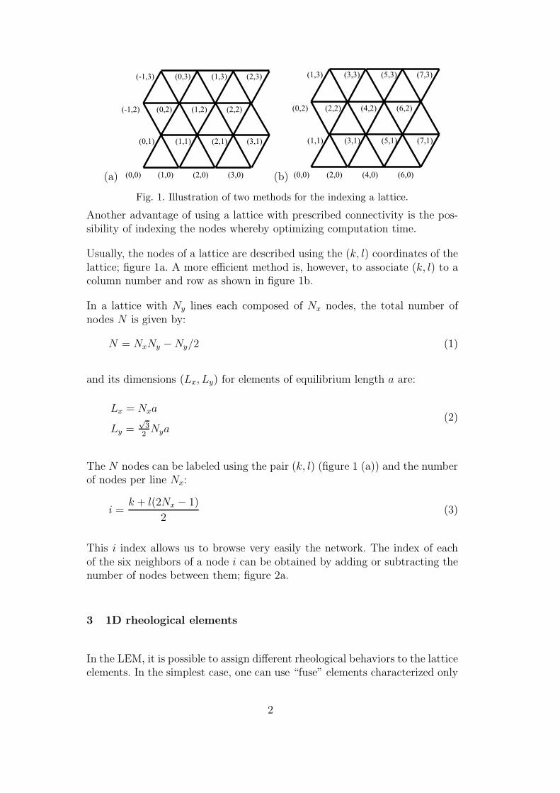
Fig. 1. Illustration of two methods for the indexing a lattice.

Another advantage of using a lattice with prescribed connectivity is the pos-sibility of indexing the nodes whereby optimizing computation time.

Usually, the nodes of a lattice are described using the (k, l) coordinates of thelattice; figure 1a. A more efficient method is, however, to associate (k, l) to acolumn number and row as shown in figure 1b.

In a lattice with Ny lines each composed of Nx nodes, the total number ofnodes N is given by:

N = NxNy −Ny/2 (1)

and its dimensions (Lx, Ly) for elements of equilibrium length a are:

Lx = Nxa

Ly =√

3

2Nya

(2)

The N nodes can be labeled using the pair (k, l) (figure 1 (a)) and the numberof nodes per line Nx:

i =k + l(2Nx − 1)

2(3)

This i index allows us to browse very easily the network. The index of eachof the six neighbors of a node i can be obtained by adding or subtracting thenumber of nodes between them; figure 2a.

3 1D rheological elements

In the LEM, it is possible to assign different rheological behaviors to the latticeelements. In the simplest case, one can use “fuse” elements characterized only

2

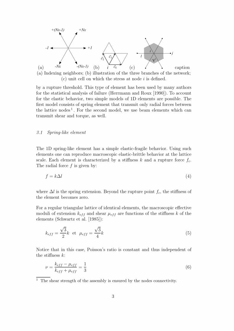
(a) (b) (c) caption(a) Indexing neighbors; (b) illustration of the three branches of the network;

(c) unit cell on which the stress at node i is defined.

by a rupture threshold. This type of element has been used by many authorsfor the statistical analysis of failure (Herrmann and Roux [1990]). To accountfor the elastic behavior, two simple models of 1D elements are possible. Thefirst model consists of spring element that transmit only radial forces betweenthe lattice nodes 1 . For the second model, we use beam elements which cantransmit shear and torque, as well.

3.1 Spring-like element

The 1D spring-like element has a simple elastic-fragile behavior. Using suchelements one can reproduce macroscopic elastic-brittle behavior at the latticescale. Each element is characterized by a stiffness k and a rupture force fc.The radial force f is given by:

f = k∆l (4)

where ∆l is the spring extension. Beyond the rupture point fc, the stiffness ofthe element becomes zero.

For a regular triangular lattice of identical elements, the macroscopic effectivemoduli of extension keff and shear µeff are functions of the stiffness k of theelements (Schwartz et al. [1985]):

keff =

√3

2k et µeff =

√3

4k (5)

Notice that in this case, Poisson’s ratio is constant and thus independent ofthe stiffness k:

ν =keff − µeff

keff + µeff

=1

3(6)

1 The shear strength of the assembly is ensured by the nodes connectivity.

3

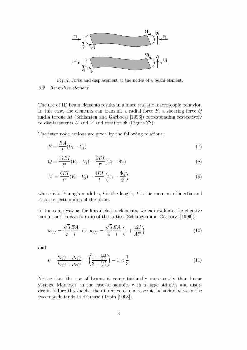
Fig. 2. Force and displacement at the nodes of a beam element.

3.2 Beam-like element

The use of 1D beam elements results in a more realistic macroscopic behavior.In this case, the elements can transmit a radial force F , a shearing force Qand a torque M (Schlangen and Garboczi [1996]) corresponding respectivelyto displacements U and V and rotation Ψ (Figure ??):

The inter-node actions are given by the following relations:

F =EA

l(Ui − Uj) (7)

Q =12EI

l3(Vi − Vj)−

6EI

l2(Ψi −Ψj) (8)

M =6EI

l2(Vi − Vj)−

4EI

l

(

Ψi −Ψj

2

)

(9)

where E is Young’s modulus, l is the length, I is the moment of inertia andA is the section area of the beam.

In the same way as for linear elastic elements, we can evaluate the effectivemoduli and Poisson’s ratio of the lattice (Schlangen and Garboczi [1996]):

keff =

√3

2

EA

let µeff =

√3

4

EA

l

(

1 +12I

Al2

)

(10)

and

ν =keff − µeff

keff + µeff

=

(

1− 12IAl2

3 + 12IAl2

)

− 1 <1

3(11)

Notice that the use of beams is computationally more costly than linearsprings. Moreover, in the case of samples with a large stiffness and disor-der in failure thresholds, the difference of macroscopic behavior between thetwo models tends to decrease (Topin [2008]).

4

4 Numerical resolution

For the numerical resolution, the initial state is considered as the referencestate. Forces and/or displacements can be applied to the boundary of thenumerical sample. We assume that the displacements are small compared tothe initial length of the elements. Different algorithms can be used to determinethe equilibrium position of all nodes, e.g. by assigning a mass to the nodesone can use dynamic algorithms as in DEM.

In this section, an alternative quasistatic approach is presented. This approachis based on a minimization of the total potential energy of the system. Theminimization is achieved through a conjugate gradient algorithm which has theadvantage of being stable and fast. The first resolution step is to calculate thetotal potential energy of the system and its gradient. The sum of the energies iscalculated along the three axes (~e0,~e1,~e2) of the lattice using i index, see figure2b. In the following, we consider both cases of spring and beam elements.

4.1 Spring elements

The degrees of freedom of the system are the node displacements ~ri. Denotingthe initial position by ~Ri, the relative displacements are:

~∆i = ~ri − ~Ri (12)

At equilibrium, we define the square distance l2ij between a node i and itsneighbor j:

l2ij + qij ≡ (~rj − ~ri)2 = (∆xj −∆xi + lxij)

2 + (∆yj −∆yi + lyij)2 (13)

with ∆ix ≡ ~∆i.~ex, ∆iy ≡ ~∆k,l.~ey and where√

l2ij + qij is the Euclidean distancebetween i and j.

To simplify the notations, we consider the case of an element between twonodes i and j. For a linear elastic stiffness k undergoing an extension ∆l, theelastic energy U is:

U =1

2k∆l2 (14)

The potential energy is given by:

Uij =1

2k(√

l2 + q − l)2

(15)

5

The gradient of energy in the orthonormal global frame (0, x, y) is given by:

~∇Uij =

δUij/δx

δUij/δy

(16)

The new equilibrium can then be determined by minimizing the total potentialenergy:

Utot =∑

i,j,

Uij (17)

4.2 Beam element

The potential energy U of a beam is given by the energies associated withradial F and transverse Q forces and momentum M (Timoshenko [1968]):

U = UF + UQ + UM =1

2

l∫

0

(

F 2

AE+

Q2

kcGA+M2

EI

)

dx (18)

where G = E/2(1 + ν) is the shear modulus, ν the Poisson ratio of the beamand kc = (10 + 10ν)/(12 + 11ν) the Timoshenko’s coefficient of transverseshear modified by (Cowper [1966]) for a beam of rectangular section.

Assuming that F ,Q andM are constant and do not depend on the longitudinalaxis x, we have:

UF =F 2

2AEl , UQ =

Q2

2kcGAl and UM =

M2

2EIl (19)

We define the axial ∆l = Ui − Uj and transversal ∆h = Vi − Vj extensions aswell as the angular variations ∆Ψ = Ψi −Ψj and ∆Ψ2 = Ψi −Ψj/2 from thenode displacements.

For beams of square section of thickness b, we introduce a coefficient Cr definedas the ratio of the beam’s thickness to its length:

Cr =b

let C2

r =A

l2(20)

6

Thus, the potential energy of a beam element can be written as the sum ofthe three following terms:

UF =1

2ElC2

r∆l2 (21)

UQ =(12 + 11ν)EC6

r l3

40

(

2

l∆h−∆Ψ

)2

(22)

UM =EC4

r l3

6

(

3

l∆h− 2∆Ψ2

)2

(23)

In the cylindrical global frame (0, x, y, φ), the gradient is given by:

~∇Uij =

δUij/δx

δUij/δy

δUij/δφ

(24)

From these equations we obtain the total potential energy of the system bysumming all the potential energies of different elements.

4.3 Failure

An advantage of the LEM is to allow for the computation of the crack pathin a simple way. Indeed, cracking is directly implemented at the level of theelements through a rupture threshold. Consider, for example, a failure criterionbased on the radial force F . During the simulation, for each strain step, theradial forces are calculated in all elements after balancing the system (byminimizing the potential energy). In principle, the strain step should be smallenough so that only one element will reach its threshold at a time (F > Fc).Since this would require very small strain increments, one of the followingtechniques can be used instead:

• when there are several critical elements with F > Fc, only the most criticalelement (with the largest force) is broken,

• All elements exceeding the force threshold Fc are broken.

To reduce the computation time, the second choice is more relevant. However,relaxation cycles should be performed at each increment to reach equilibriumbefore applying the next load increment. These relaxation cycles allow for thepropagation of a crack within a single strain step. This physically correspondsto instantaneous propagation of cracks at imposed strain rate.

7

0 50 100 150 200 250 300 350N

x

0.5

0.6

0.7

0.8

0.9

1.0

E

(a)0 50 100 150 200 250 300 350

Nx

6

8

10

12

σ Y (

.10-3

)

(b)

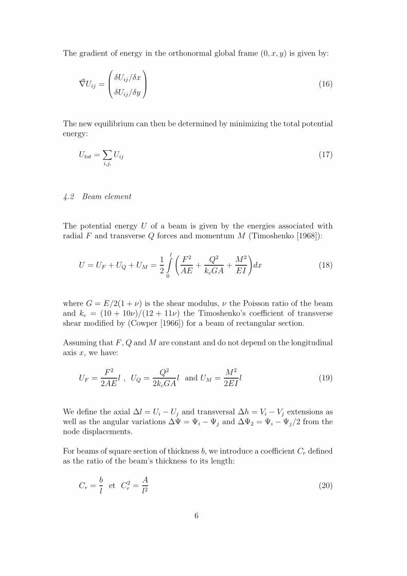
Fig. 3. Young modulus (a) and failure stress (b) as a function of the size Nx ofsample.

5 Influence of meshing

We study here the influence of the mesh on the Young modulus and tensilestrength of the lattice. This influence affects not only the number of cells thatare involved in the simulation but also the geometrical disorder and stiffnessintroduced at the level of the elements.

5.1 Finite size effects

Figure 3 shows the Young modulus E and the failure stress σY of a homoge-neous square sample (Nx = Ny) loaded in uniaxial tension as a function ofsample size. We use a regular triangular lattice of spring elements (stiffnessk = 1, initial length l = 1).

We see that E and σY rapidly converge to a constant. This value equals to√3/2 for the Young modulus. The failure threshold σY is well defined for

Nx > 50. In practice, for a system composed of many particles, it is thereforenecessary to use approximately 502 = 2500 nodes in each particle.

5.2 Disordered mesh

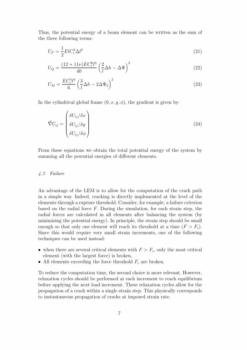
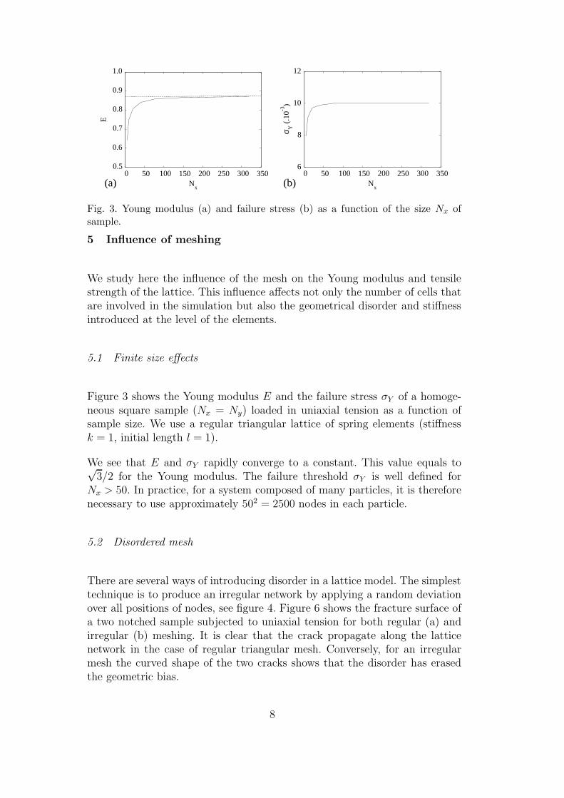
There are several ways of introducing disorder in a lattice model. The simplesttechnique is to produce an irregular network by applying a random deviationover all positions of nodes, see figure 4. Figure 6 shows the fracture surface ofa two notched sample subjected to uniaxial tension for both regular (a) andirregular (b) meshing. It is clear that the crack propagate along the latticenetwork in the case of regular triangular mesh. Conversely, for an irregularmesh the curved shape of the two cracks shows that the disorder has erasedthe geometric bias.

8

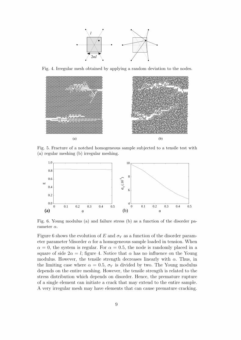
Fig. 4. Irregular mesh obtained by applying a random deviation to the nodes.

Fig. 5. Fracture of a notched homogeneous sample subjected to a tensile test with(a) regular meshing (b) irregular meshing.

0 0.1 0.2 0.3 0.4 0.5

α

0.0

0.2

0.4

0.6

0.8

1.0

E

(a)(a)0 0.1 0.2 0.3 0.4 0.5

α

4

6

8

10

σ Y (.

10-3

)

(b)

Fig. 6. Young modulus (a) and failure stress (b) as a function of the disorder pa-rameter α.

Figure 6 shows the evolution of E and σY as a function of the disorder param-eter parameter !disorder α for a homogeneous sample loaded in tension. Whenα = 0, the system is regular. For α = 0.5, the node is randomly placed in asquare of side 2α = l; figure 4. Notice that α has no influence on the Youngmodulus. However, the tensile strength decreases linearly with α. Thus, inthe limiting case where α = 0.5, σY is divided by two. The Young modulusdepends on the entire meshing. However, the tensile strength is related to thestress distribution which depends on disorder. Hence, the premature ruptureof a single element can initiate a crack that may extend to the entire sample.A very irregular mesh may have elements that can cause premature cracking.

9

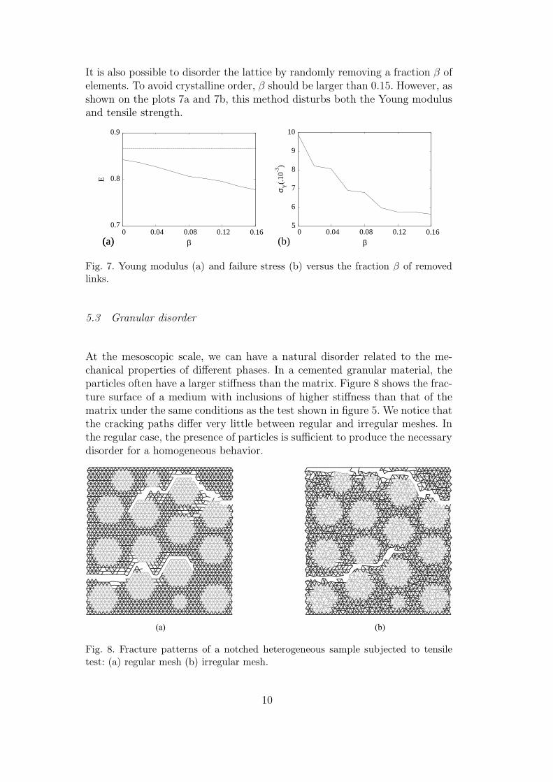
It is also possible to disorder the lattice by randomly removing a fraction β ofelements. To avoid crystalline order, β should be larger than 0.15. However, asshown on the plots 7a and 7b, this method disturbs both the Young modulusand tensile strength.

0 0.04 0.08 0.12 0.16

β

0.7

0.8

0.9

E

(a)(a)0 0.04 0.08 0.12 0.16

β

5

6

7

8

9

10

σ Y(.

10-3

)

(b)

Fig. 7. Young modulus (a) and failure stress (b) versus the fraction β of removedlinks.

5.3 Granular disorder

At the mesoscopic scale, we can have a natural disorder related to the me-chanical properties of different phases. In a cemented granular material, theparticles often have a larger stiffness than the matrix. Figure 8 shows the frac-ture surface of a medium with inclusions of higher stiffness than that of thematrix under the same conditions as the test shown in figure 5. We notice thatthe cracking paths differ very little between regular and irregular meshes. Inthe regular case, the presence of particles is sufficient to produce the necessarydisorder for a homogeneous behavior.

Fig. 8. Fracture patterns of a notched heterogeneous sample subjected to tensiletest: (a) regular mesh (b) irregular mesh.

10

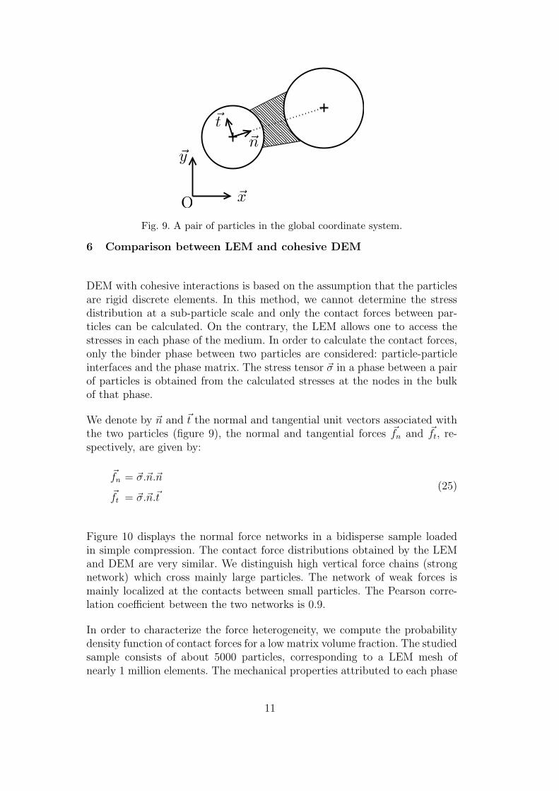
Fig. 9. A pair of particles in the global coordinate system.

6 Comparison between LEM and cohesive DEM

DEM with cohesive interactions is based on the assumption that the particlesare rigid discrete elements. In this method, we cannot determine the stressdistribution at a sub-particle scale and only the contact forces between par-ticles can be calculated. On the contrary, the LEM allows one to access thestresses in each phase of the medium. In order to calculate the contact forces,only the binder phase between two particles are considered: particle-particleinterfaces and the phase matrix. The stress tensor ~σ in a phase between a pairof particles is obtained from the calculated stresses at the nodes in the bulkof that phase.

We denote by ~n and ~t the normal and tangential unit vectors associated withthe two particles (figure 9), the normal and tangential forces ~fn and ~ft, re-spectively, are given by:

~fn = ~σ.~n.~n

~ft = ~σ.~n.~t(25)

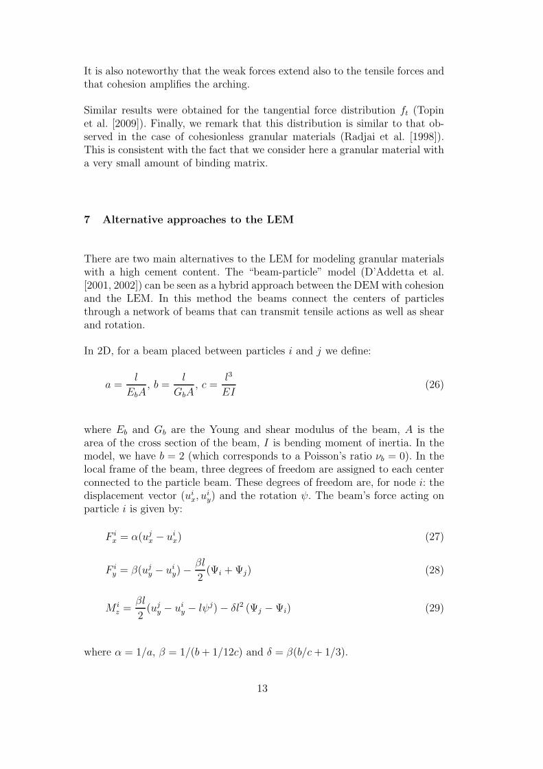
Figure 10 displays the normal force networks in a bidisperse sample loadedin simple compression. The contact force distributions obtained by the LEMand DEM are very similar. We distinguish high vertical force chains (strongnetwork) which cross mainly large particles. The network of weak forces ismainly localized at the contacts between small particles. The Pearson corre-lation coefficient between the two networks is 0.9.

In order to characterize the force heterogeneity, we compute the probabilitydensity function of contact forces for a low matrix volume fraction. The studiedsample consists of about 5000 particles, corresponding to a LEM mesh ofnearly 1 million elements. The mechanical properties attributed to each phase

11

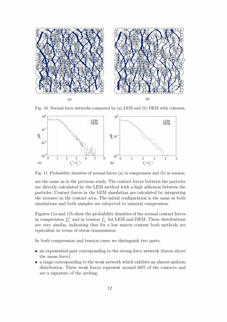
Fig. 10. Normal force networks computed by (a) LEM and (b) DEM with cohesion.

0 1 2 3 4 5 6

fn

+/<f

n

+>

10-3

10-2

10-1

100

pdf

LEMDEM

(a)0 1 2 3 4 5

fn

-/<f

n

->

10-2

10-1

100

pdf

LEMDEM

(b)

Fig. 11. Probability densities of normal forces (a) in compression and (b) in tension.

are the same as in the previous study. The contact forces between the particlesare directly calculated by the LEM method with a high adhesion between theparticles. Contact forces in the LEM simulation are calculated by integratingthe stresses on the contact area. The initial configuration is the same in bothsimulations and both samples are subjected to uniaxial compression.

Figures 11a and 11b show the probability densities of the normal contact forcesin compression f+

n and in tension f−

n for LEM and DEM. These distributionsare very similar, indicating that for a low matrix content both methods areequivalent in terms of stress transmission.

In both compression and tension cases we distinguish two parts:

• an exponential part corresponding to the strong force network (forces abovethe mean force)

• a range corresponding to the weak network which exhibits an almost uniformdistribution. These weak forces represent around 60% of the contacts andare a signature of the arching.

12

It is also noteworthy that the weak forces extend also to the tensile forces andthat cohesion amplifies the arching.

Similar results were obtained for the tangential force distribution ft (Topinet al. [2009]). Finally, we remark that this distribution is similar to that ob-served in the case of cohesionless granular materials (Radjai et al. [1998]).This is consistent with the fact that we consider here a granular material witha very small amount of binding matrix.

7 Alternative approaches to the LEM

There are two main alternatives to the LEM for modeling granular materialswith a high cement content. The “beam-particle” model (D’Addetta et al.[2001, 2002]) can be seen as a hybrid approach between the DEM with cohesionand the LEM. In this method the beams connect the centers of particlesthrough a network of beams that can transmit tensile actions as well as shearand rotation.

In 2D, for a beam placed between particles i and j we define:

a =l

EbA, b =

l

GbA, c =

l3

EI(26)

where Eb and Gb are the Young and shear modulus of the beam, A is thearea of the cross section of the beam, I is bending moment of inertia. In themodel, we have b = 2 (which corresponds to a Poisson’s ratio νb = 0). In thelocal frame of the beam, three degrees of freedom are assigned to each centerconnected to the particle beam. These degrees of freedom are, for node i: thedisplacement vector (uix, u

iy) and the rotation ψ. The beam’s force acting on

particle i is given by:

F ix = α(ujx − uix) (27)

F iy = β(ujy − uiy)−

βl

2(Ψi +Ψj) (28)

M iz =

βl

2(ujy − uiy − lψj)− δl2 (Ψj −Ψi) (29)

where α = 1/a, β = 1/(b+ 1/12c) and δ = β(b/c+ 1/3).

13

In this model, the failure is taken into account using the criterion:

pb =

(

ǫbǫb,max

)2

+max (|ψi| , |ψj|)

ψmax

≥ 1 (30)

where ǫb =∆llis the longitudinal deformation of the beam and ǫb,max and ψmax

are the failure thresholds.

A second alternative model is to use a “cohesive zone” approach (Raous et al.[1999]) associated with a discrete element method (Pelissou et al. [2009]).In this approach, it is possible to integrate a complex behavior at interfacesbetween particles. A major drawback of this type of methods is that the com-putation time greatly depends on the number of cohesive zones taken intoaccount and that these zones have predefined crack paths. Moreover, thismethod can not easily simulate the case of materials with strong gradients ofproperties.

References

G.R. Cowper. The shear coefficient in timoshenko’s beam theory. ASME

Journal of Applied Mechanics, 33:335–340, 1966.G. A. D’Addetta, F. Kun, E. Ramm, and H. J. Herrmann. Continuous and

discontinuous modelling of cohesive frictional materials, chapter From solidsto granulates – Discrete element simulations of fracture and fragmentationprocesses in geomaterials, pages 231–258. Springer, 2001.

G. A. D’Addetta, F. Kun, and E. Ramm. On the application of a discretemodel to the fracture process of cohesive granular materials. Granular Mat-

ter, 4:77–90, 2002.H. J. Herrmann and S. Roux, editors. Statistical Models for Fracture in Dis-

ordered Media. North Holland, Amsterdam, 1990.C. Pelissou, J. Baccou, Y. Monerie, and F. Perales. Determination of the sizeof the representative volume element for random quasi-brittle composites.International Journal of Solids and Structures, 46(14-15):2842–2855, 2009.

F. Radjai, D. E. Wolf, M. Jean, and J. J. Moreau. Bimodal character of stresstransmission in granular packings. Phys. Rev. Lett., 80(1):61–64, 1998.

M. Raous, L. Cangemi, and M. Cocu. A consistent model coupling adhesion,friction, and unilateral contact. Computer Methods in Applied Mechanics

and Engineering, 177(3-4):383–399, 1999.E. Schlangen and E. J. Garboczi. New method for simulating fracture usingan elastically uniform random geometry lattice. International Journal of

Engineering Science, 34(10):1131–1144, 1996.Lawrence M. Schwartz, Shechao Feng, M. F. Thorpe, and Pabitra N. Sen.

14

Behavior of depleted elastic networks: Comparison of effective-medium andnumerical calculations. Phys. Rev. B, 32(7):4607–, 1985.

S.P. Timoshenko. Resistance des materiaux. Dunod, Paris, 1968.V. Topin. Materiaux granulaires cimentes : modelisation et application a

l’albumen de ble. PhD thesis, Universite Montpellier 2, 2008.V. Topin, F. Radjai, and J. Y. Delenne. Subparticle stress fields in granularsolids. Physical Review E, 79(5), 2009.

15