Embed Size (px)
Citation preview
Latin – Laplace Inversion Tool
User Guide
B Snowball
QRS-4007A-T2-9
Version 1.0
July 2014
Quintessa Limited Tel: +44 (0) 1491 636246 The Hub, 14 Station Road Fax: +44 (0) 1491 636247 Henley-on-Thames [email protected] Oxfordshire RG9 1AY www.quintessa.org United Kingdom www.quintessa-online.com
Document History
Title: Latin – Laplace Inversion Tool
Subtitle: User Guide
Client: Quintessa Limited
Document Number: QRS-4007A-T2-9
Version Number: Version 1.0 Date: July 2014
Notes:
Prepared by: B Snowball
Reviewed by: Thomas Williams, Paul Suckling
Approved by: Paul Suckling
Latin User Guide
i
Summary
This is the user guide for Version 1.0 of Latin, a graphical user interface for numerically
inverting Laplace transforms and viewing results in a tabular or graphical format. The
numerical inversion is carried out using the Talbot algorithm.
Latin is designed to allow both quick inversion of simple one-line transforms, and
inversion of more complex expressions with units and units checking.

Latin User Guide
iii
Contents
1 Introduction 1
2 The Algorithm 1
2.1 The Talbot Method 1
2.1.1 Constraints 2
2.1.2 Limitations 2
3 Starting with Latin 7
4 Quick Inversions 7
4.1 Preparing a Laplace Transform to Invert 8
4.1.1 The Laplace Transform 8
4.1.2 Time over which to Plot 9
4.1.3 Advanced Controls 9
4.2 Calculating 10
4.2.1 Unsuccessful Calculation 10
5 Successful Calculation 11
5.1.1 Results Table 11
5.1.2 Graphs 12
6 Advanced Latin 13
6.1 Writing a New File 13
6.1.1 Parameters 14
6.1.2 Laplace Inversions 20
6.1.3 Report Times 20
6.1.4 Report Parameters 23
6.1.5 Controls 23
6.2 Saving a file 24
6.3 Loading a file with Latin 24
6.4 Running a file 25
6.4.1 Unsuccessful Calculation 26
6.5 Enabling Dimensions/Units (turning off the default “Dimensionless” mode) 27
6.5.1 Laplace Transform Inversions with Units 28
6.5.2 Output Time Unit 28
6.5.3 Syntax for Units 28
6.5.4 Parameter Procedures 31
6.6 Loading and Running Externally Created Input Files 32
6.7 Output files 33
References 33

Latin User Guide
1
1 Introduction
This is the user guide for Version 1.0 of Latin, a graphical user interface for numerically
inverting Laplace transforms and viewing results in a tabular or graphical format. The
numerical inversion is carried out using the Talbot algorithm.
Latin is designed to allow both quick inversion of simple one-line transforms, and
inversion of more complex expressions with units and units checking.
2 The Algorithm
Currently, Latin only uses one Laplace Transform inversion method, the method
proposed by Talbot (1979), and also detailed and discussed in Robinson and Maul
(1991).
2.1 The Talbot Method
The inversion formula for the inverse Laplace Transform of 𝑓̅(𝑠) is given by
𝑓(𝑡) = 1
2𝜋𝑖∫ 𝑒𝑠𝑡𝑓(̅𝑠) 𝑑𝑠
𝐵
,
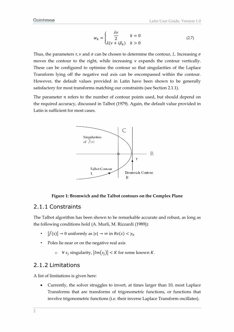
where 𝐵 is the Bromwich contour from 𝛾 − 𝑖∞ to 𝛾 + 𝑖∞ with 𝛾 > 𝛾0 (see Figure 1). The
Talbot method involves deforming the contour, and using a trapezoidal approximation
for the integral. This new contour is shown also in Figure 1 as the curve L.
The Talbot inversion formula used in Latin’s solver is defined as follows:
𝑓(𝑡) ≈
1
𝑛∑ ℜ[𝑤𝑘𝑒𝑠𝑘𝑡𝑓(̅𝑠𝑘) ]
𝑛−1
𝑘=0
(2.1)
where ℜ denotes the real part of, and
𝜃𝑘 =
𝑘𝜋
𝑛 (2.2)
𝜆 =𝜏
𝑡 (2.3)
𝛼𝑘 = 𝜃𝑘 cot(𝜃𝑘) (2.4)
𝛽𝑘 = 𝜃𝑘 +
𝛼𝑘(𝛼𝑘 − 1)
𝜃𝑘 (2.5)
𝑠𝑘 = 𝜆(𝛼𝑘 + 𝑖𝜈𝜃𝑘) + 𝜎 (2.6)
Latin User Guide, Version 1.0
2
𝑤𝑘 = {
𝜆𝜈
2𝑘 = 0
𝜆(𝜈 + 𝑖𝛽𝑘) 𝑘 > 0 (2.7)
Thus, the parameters 𝜏, 𝜈 and 𝜎 can be chosen to determine the contour, L. Increasing 𝜎
moves the contour to the right, while increasing 𝜈 expands the contour vertically.
These can be configured to optimise the contour so that singularities of the Laplace
Transform lying off the negative real axis can be encompassed within the contour.
However, the default values provided in Latin have been shown to be generally
satisfactory for most transforms matching our constraints (see Section 2.1.1).
The parameter 𝑛 refers to the number of contour points used, but should depend on
the required accuracy, discussed in Talbot (1979). Again, the default value provided in
Latin is sufficient for most cases.
Figure 1: Bromwich and the Talbot contours on the Complex Plane
2.1.1 Constraints
The Talbot algorithm has been shown to be remarkable accurate and robust, as long as
the following conditions hold (A. Murli, M. Rizzardi (1989)):
• |𝑓̅(s)| → 0 uniformly as |𝑠| → ∞ in 𝑅𝑒(𝑠) < 𝛾0
• Poles lie near or on the negative real axis
o ∀ 𝑠𝑗 singularity, |𝐼𝑚(𝑠𝑗)| < 𝐾 for some known 𝐾.
2.1.2 Limitations
A list of limitations is given here:
Currently, the solver struggles to invert, at times larger than 10, most Laplace
Transforms that are transforms of trigonometric functions, or functions that
involve trigonometric functions (i.e. their inverse Laplace Transform oscillates).
Latin User Guide
3
Occasionally, when the solver is trying to calculate a value that is close to 0, it
will struggle to deduce this answer since its own inner error checks will
produce an error larger than its allowed tolerance (since any percentage
difference between a number close to zero and zero is large). When this occurs,
Latin will produce “***” as the output at these times, which in graphs is taken
as 0.
If a Laplace Transform inverts to an exponentially growing function, then the
solver may struggle to deal with the speed of the growth.
Latin cannot invert the Dirac delta function successfully.
Latin can detect the Heaviside function if it is not used to premulitply another
function. When it is used to premulitply a function, the time delay is recognised
but output for times less than the critical time contain “***” instead of 0.
Effects of Varying Talbot Parameters
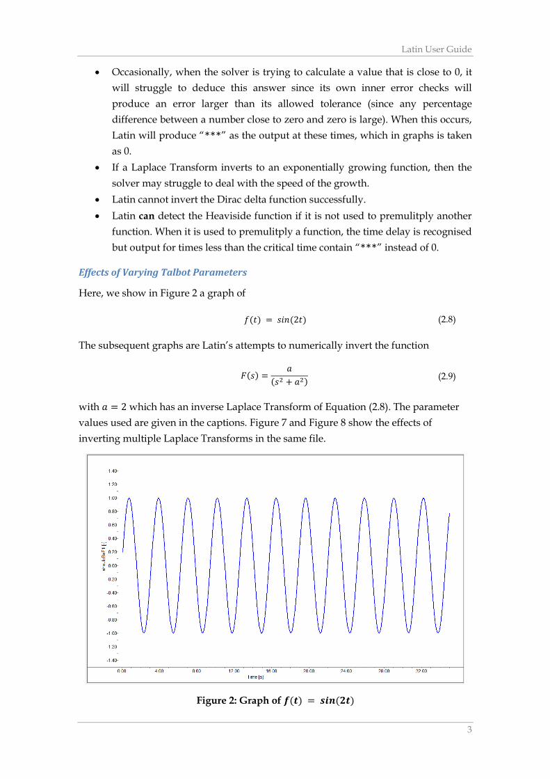
Here, we show in Figure 2 a graph of
𝑓(𝑡) = 𝑠𝑖𝑛(2𝑡) (2.8)
The subsequent graphs are Latin’s attempts to numerically invert the function
𝐹(𝑠) =𝑎
(𝑠2 + 𝑎2) (2.9)
with 𝑎 = 2 which has an inverse Laplace Transform of Equation (2.8). The parameter
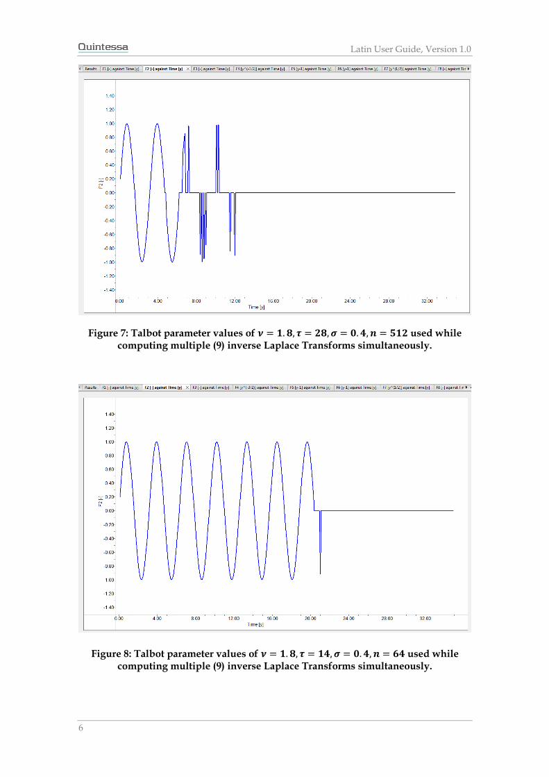
values used are given in the captions. Figure 7 and Figure 8 show the effects of
inverting multiple Laplace Transforms in the same file.
Figure 2: Graph of 𝒇(𝒕) = 𝒔𝒊𝒏(𝟐𝒕)
Latin User Guide, Version 1.0
4
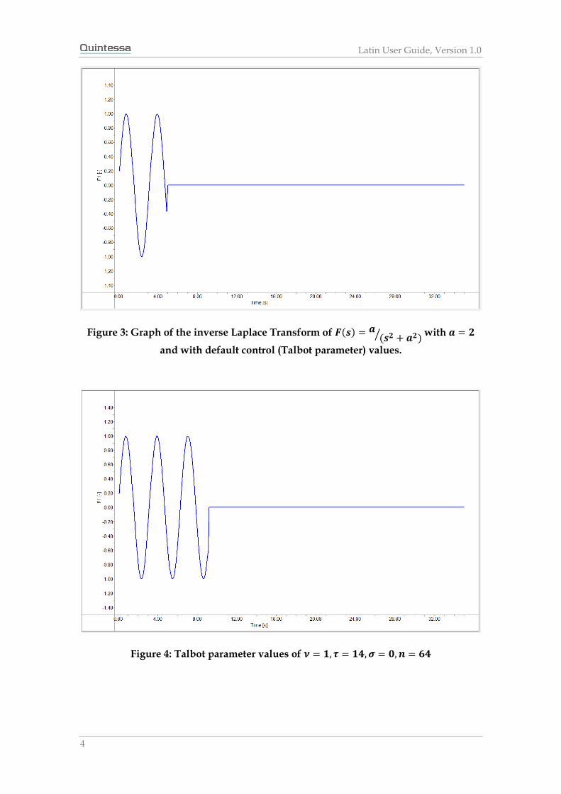
Figure 3: Graph of the inverse Laplace Transform of 𝑭(𝒔) = 𝒂(𝒔𝟐 + 𝒂𝟐)⁄ with 𝒂 = 𝟐
and with default control (Talbot parameter) values.
Figure 4: Talbot parameter values of 𝝂 = 𝟏, 𝝉 = 𝟏𝟒, 𝝈 = 𝟎, 𝒏 = 𝟔𝟒
Latin User Guide
5
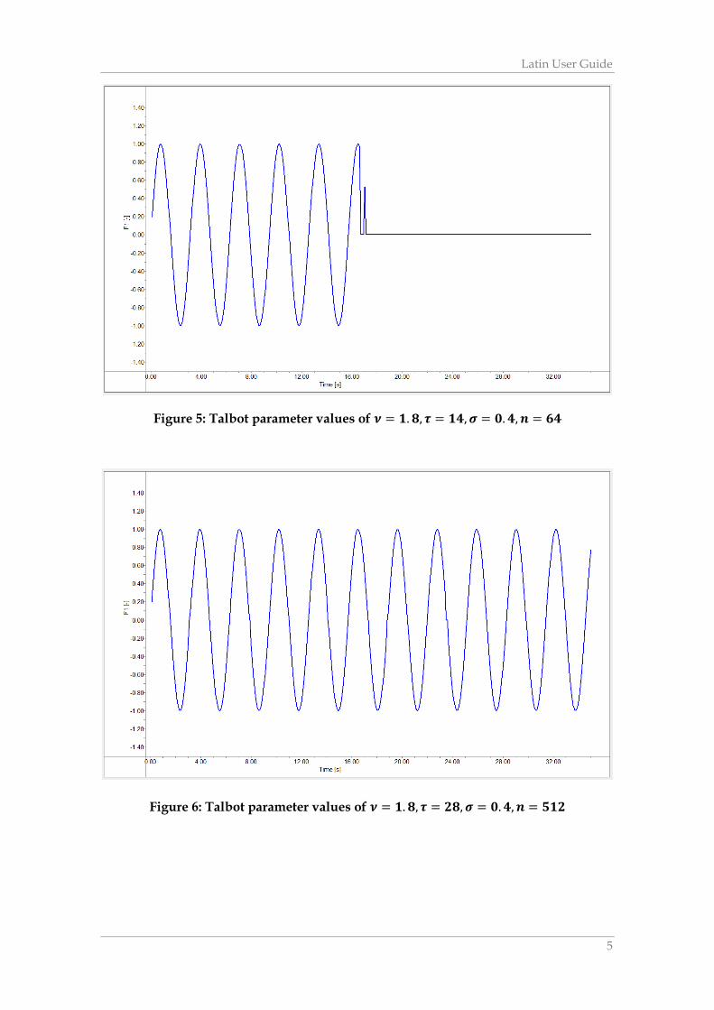
Figure 5: Talbot parameter values of 𝝂 = 𝟏. 𝟖, 𝝉 = 𝟏𝟒, 𝝈 = 𝟎. 𝟒, 𝒏 = 𝟔𝟒
Figure 6: Talbot parameter values of 𝝂 = 𝟏. 𝟖, 𝝉 = 𝟐𝟖, 𝝈 = 𝟎. 𝟒, 𝒏 = 𝟓𝟏𝟐
Latin User Guide, Version 1.0
6
Figure 7: Talbot parameter values of 𝝂 = 𝟏. 𝟖, 𝝉 = 𝟐𝟖, 𝝈 = 𝟎. 𝟒, 𝒏 = 𝟓𝟏𝟐 used while computing multiple (9) inverse Laplace Transforms simultaneously.
Figure 8: Talbot parameter values of 𝝂 = 𝟏. 𝟖, 𝝉 = 𝟏𝟒, 𝝈 = 𝟎. 𝟒, 𝒏 = 𝟔𝟒 used while computing multiple (9) inverse Laplace Transforms simultaneously.
Latin User Guide
7
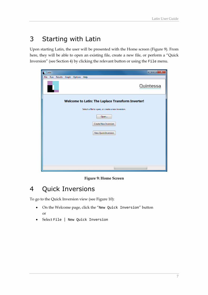
3 Starting with Latin
Upon starting Latin, the user will be presented with the Home screen (Figure 9). From
here, they will be able to open an existing file, create a new file, or perform a “Quick
Inversion” (see Section 4) by clicking the relevant button or using the File menu.
Figure 9: Home Screen
4 Quick Inversions
To go to the Quick Inversion view (see Figure 10):
On the Welcome page, click the “New Quick Inversion” button
or
Select File | New Quick Inversion
Latin User Guide, Version 1.0
8
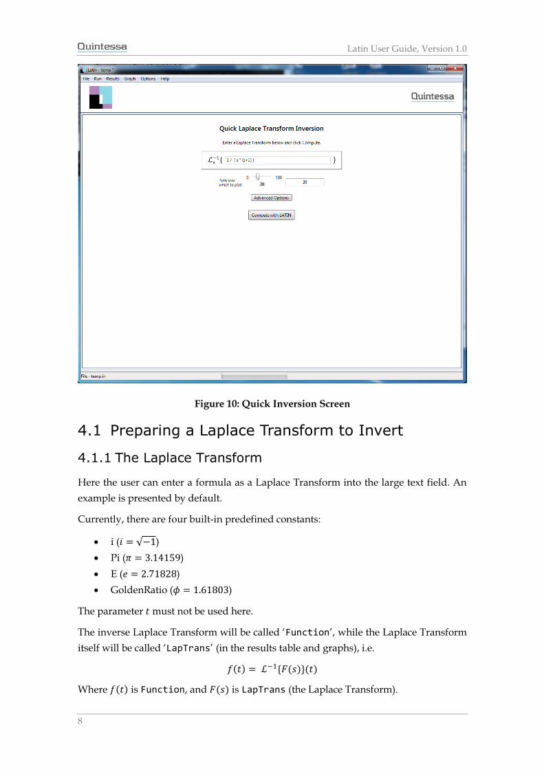
Figure 10: Quick Inversion Screen
4.1 Preparing a Laplace Transform to Invert
4.1.1 The Laplace Transform
Here the user can enter a formula as a Laplace Transform into the large text field. An
example is presented by default.
Currently, there are four built-in predefined constants:
i (𝑖 = √−1)
Pi (𝜋 = 3.14159)
E (𝑒 = 2.71828)
GoldenRatio (𝜙 = 1.61803)
The parameter 𝑡 must not be used here.
The inverse Laplace Transform will be called ‘Function’, while the Laplace Transform
itself will be called ‘LapTrans’ (in the results table and graphs), i.e.
𝑓(𝑡) = ℒ−1{𝐹(𝑠)}(𝑡)
Where 𝑓(𝑡) is Function, and 𝐹(𝑠) is LapTrans (the Laplace Transform).
Latin User Guide
9
4.1.2 Time over which to Plot
Below the Laplace Transform, the user can choose to specify the time over which to
plot. This will run the calculation and produce output at a range of times between 0
and the time entered here. While the slider will allow integer values between 0 and
100, any positive number can be entered into the text box field – however the user
should not enter a large number here (>100) since Latin will take a long time to
compute and may have to be manually terminated.
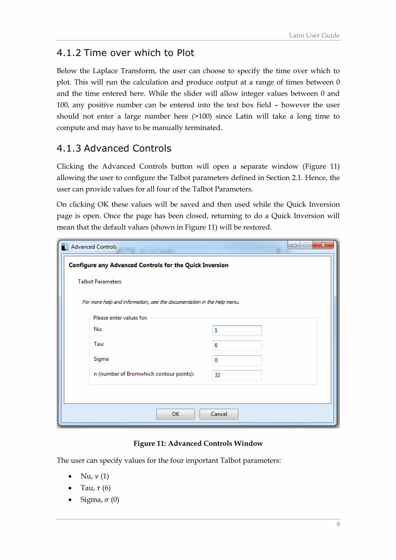
4.1.3 Advanced Controls
Clicking the Advanced Controls button will open a separate window (Figure 11)
allowing the user to configure the Talbot parameters defined in Section 2.1. Hence, the
user can provide values for all four of the Talbot Parameters.
On clicking OK these values will be saved and then used while the Quick Inversion
page is open. Once the page has been closed, returning to do a Quick Inversion will
mean that the default values (shown in Figure 11) will be restored.
Figure 11: Advanced Controls Window
The user can specify values for the four important Talbot parameters:
Nu, 𝜈 (1)
Tau, 𝜏 (6)
Sigma, 𝜎 (0)
Latin User Guide, Version 1.0
10
Number of Bromwich contour points, 𝑛 (32)
Nu, Tau and Sigma can be any real number, whereas n must be an integer. The default
values given are in brackets above, and provide suitable values for the parameters for
most inversions. However, expert users are welcome to alter these values in order to
increase accuracy or reduce the number of failed report values.
4.2 Calculating
Pressing the “Compute with LATIN” button will tell Latin to start inverting the
Laplace Transform given and produce output for a range of times between 0 and the
end time specified.
Latin does this by saving the input given as a .in file in a directory inside the user’s
AppData directory called Latin. This file should not be edited or moved while the
Latin is calculating but the files will be automatically deleted upon completion.
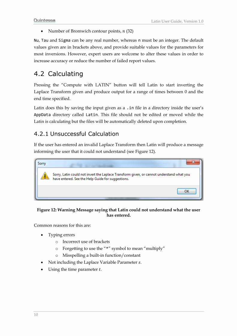
4.2.1 Unsuccessful Calculation
If the user has entered an invalid Laplace Transform then Latin will produce a message
informing the user that it could not understand (see Figure 12).
Figure 12: Warning Message saying that Latin could not understand what the user has entered.
Common reasons for this are:
Typing errors
o Incorrect use of brackets
o Forgetting to use the “*” symbol to mean “multiply”
o Misspelling a built-in function/constant
Not including the Laplace Variable Parameter 𝑠.
Using the time parameter 𝑡.
Latin User Guide
11
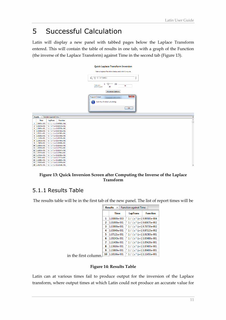
5 Successful Calculation
Latin will display a new panel with tabbed pages below the Laplace Transform
entered. This will contain the table of results in one tab, with a graph of the Function
(the inverse of the Laplace Transform) against Time in the second tab (Figure 13).
Figure 13: Quick Inversion Screen after Computing the Inverse of the Laplace Transform
5.1.1 Results Table
The results table will be in the first tab of the new panel. The list of report times will be
in the first column.
Figure 14: Results Table
Latin can at various times fail to produce output for the inversion of the Laplace
transform, where output times at which Latin could not produce an accurate value for
Latin User Guide, Version 1.0
12
the inversion will be replaced by “***”. Currently known limitations are listed in
Section 2.1.2.
Any parameter noted to contain the parameter s will just be displayed in quotes as the
formula that would give its value, since s cannot be evaluated.
There are various options in the Results menu, such as toggling whether to display the
table lines and copying the result to the computer clipboard.
Right clicking on any column heading will allow the user to create a graph of that
function against time (if applicable).
Multiple rows or multiple columns can be selected by clicking and dragging the labels
(in bold), or by using ctrl + click. A block of cells can be copied by clicking and
dragging on the desired cells. The selected cells can then be copied by right clicking the
selection and pressing Copy selection. Note that only blocks of cells can be copied, that
is, all cells must be touching and form a rectangle. All cells in the table can be copied
by right clicking and pressing Copy all.
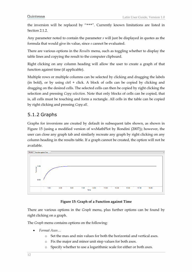
5.1.2 Graphs
Graphs for inversions are created by default in subsequent tabs shown, as shown in
Figure 15 (using a modified version of wxMathPlot by Rondini (2007)); however, the
user can close any graph tab and similarly recreate any graph by right clicking on any
column heading in the results table. If a graph cannot be created, the option will not be
available.
Figure 15: Graph of a Function against Time
There are various options in the Graph menu, plus further options can be found by
right clicking on a graph.
The Graph menu contains options on the following:
Format Axes…
o Set the max and min values for both the horizontal and vertical axes.
o Fix the major and minor unit step values for both axes.
o Specify whether to use a logarithmic scale for either or both axes.
Latin User Guide
13
Zoom In,Zoom Out and Reset Zoom
Show Grid Lines
Show Coordinate info box
o The box updates with the coordinates of the point at which the mouse is
hovering when on the graph.
Disable Mouse Controls
The pop-up menu found by right clicking on a graph contains:
Format Axes…
o Set the max and min values for both the horizontal and vertical axes.
o Fix the major and minor unit step values for both axes.
o Specify whether to use a logarithmic scale for either or both axes.
Reset the view
Centre on this point
Zoom In and Zoom Out
Lock aspect
Disable Mouse Controls
Show mouse commands…
Scrolling and zooming can also be done with the mouse and keyboard; for a list of
mouse controls, right click on a graph and select Show mouse commands…. However the
user can disable mouse controls by choosing Disable mouse controls or selecting Graph |
Disable mouse controls in the menu bar.
Each graph has its own local state, and so changing any of the options available for a
graph does so just for that single graph concerned.
To save the graph as an image, simply go to File | Save Graph Screenshot As… where the
user can save the current view of the current graph in a variety of image formats.
6 Advanced Latin
6.1 Writing a New File
To create a new file:
Go to File | New
or
Click the Create New Inversion button when at the Home screen.
Selecting to create a new file will take the user to the Latin File Editor screen. Here the
user will be presented with five pages split into different tabs that the user can toggle
between. Notice also that the “Run File” button now becomes active. Once the user
Latin User Guide, Version 1.0
14
has finished editing their file, they can run the file by pressing this button (see
Section 6.4).
Each tab allows the user to specify different items and options to create a file to run.
The pages are:
Parameters
Laplace Inversions
Report Times
Report Parameters
Controls
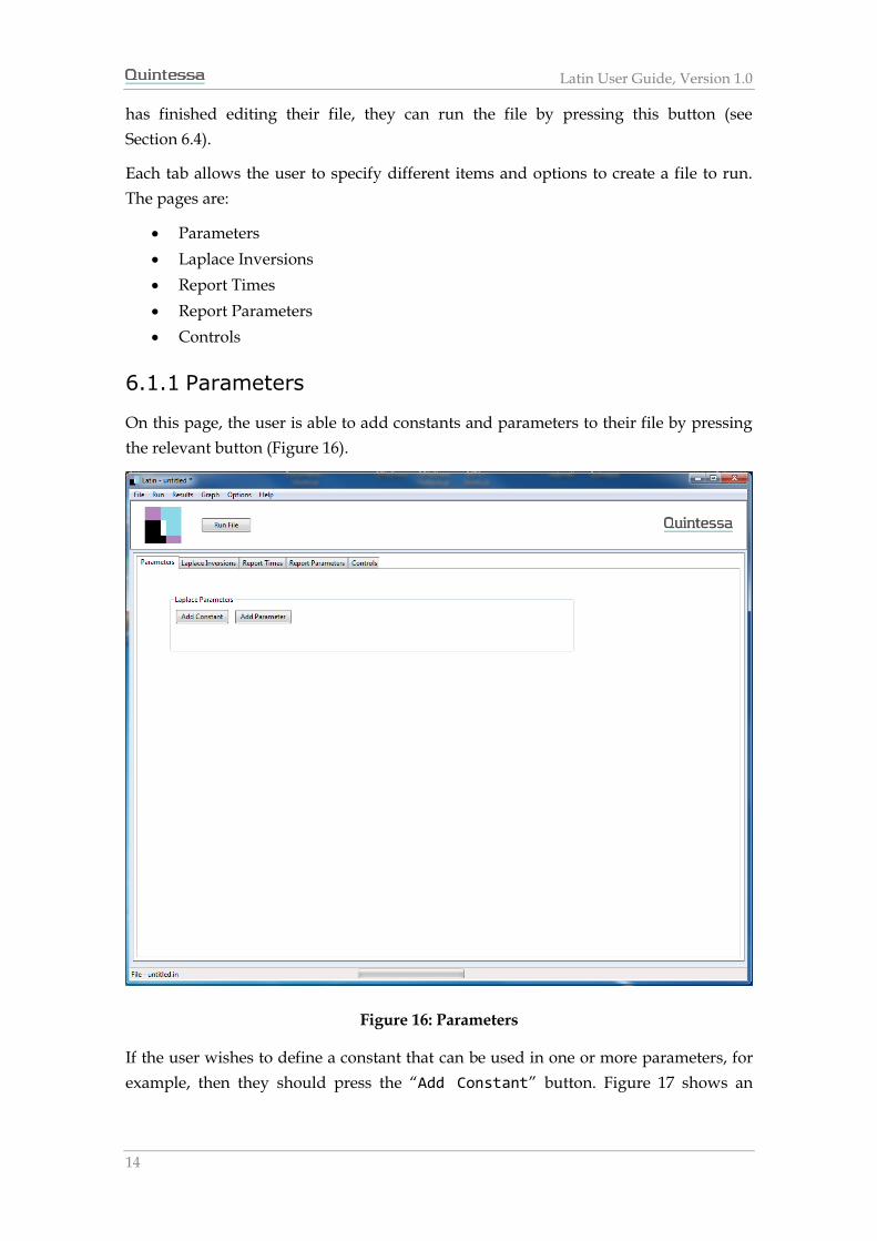
6.1.1 Parameters
On this page, the user is able to add constants and parameters to their file by pressing
the relevant button (Figure 16).
Figure 16: Parameters
If the user wishes to define a constant that can be used in one or more parameters, for
example, then they should press the “Add Constant” button. Figure 17 shows an
Latin User Guide
15
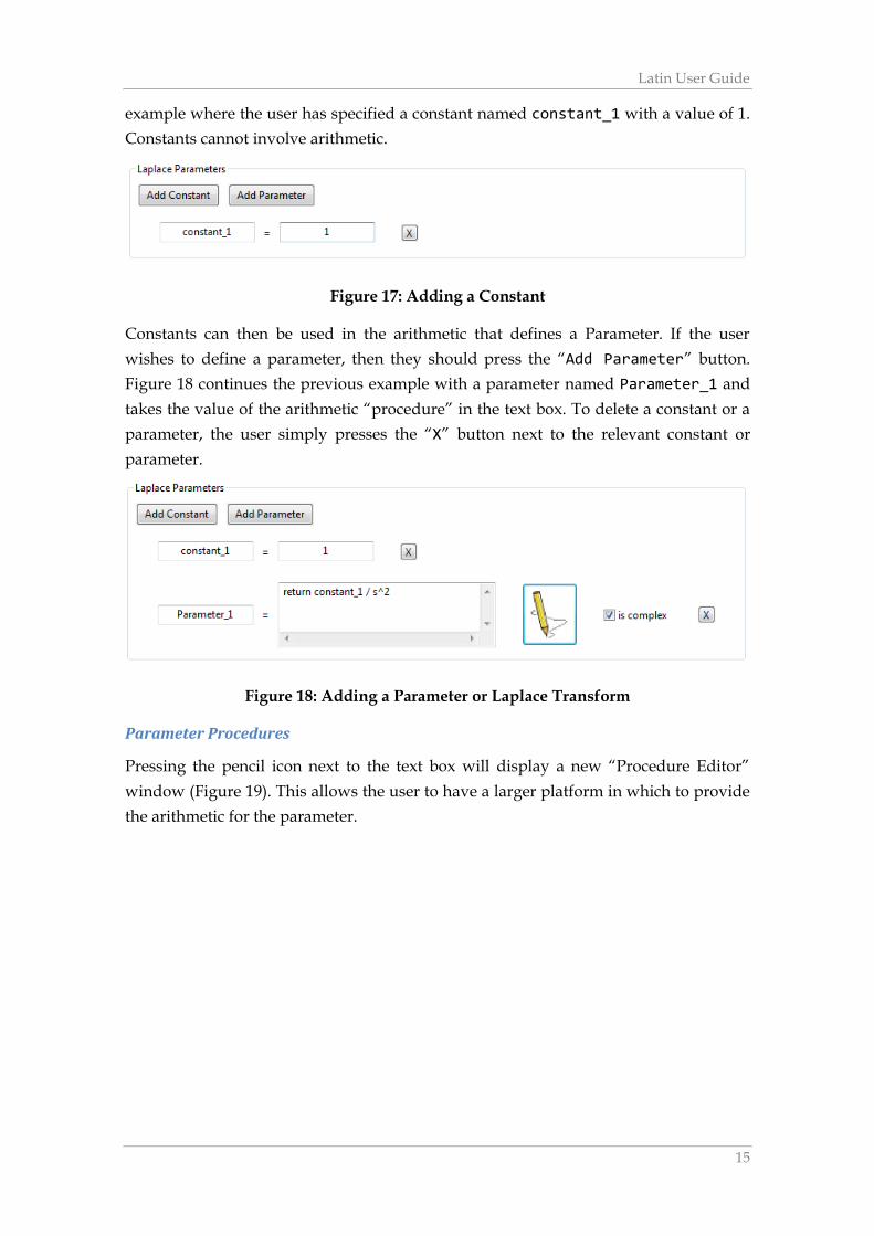
example where the user has specified a constant named constant_1 with a value of 1.
Constants cannot involve arithmetic.
Figure 17: Adding a Constant
Constants can then be used in the arithmetic that defines a Parameter. If the user
wishes to define a parameter, then they should press the “Add Parameter” button.
Figure 18 continues the previous example with a parameter named Parameter_1 and
takes the value of the arithmetic “procedure” in the text box. To delete a constant or a
parameter, the user simply presses the “X” button next to the relevant constant or
parameter.
Figure 18: Adding a Parameter or Laplace Transform
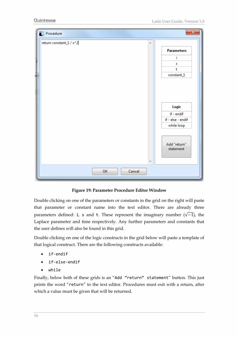
Parameter Procedures
Pressing the pencil icon next to the text box will display a new “Procedure Editor”
window (Figure 19). This allows the user to have a larger platform in which to provide
the arithmetic for the parameter.
Latin User Guide, Version 1.0
16
Figure 19: Parameter Procedure Editor Window
Double clicking on one of the parameters or constants in the grid on the right will paste
that parameter or constant name into the text editor. There are already three
parameters defined: i, s and t. These represent the imaginary number (√−1), the
Laplace parameter and time respectively. Any further parameters and constants that
the user defines will also be found in this grid.
Double clicking on one of the logic constructs in the grid below will paste a template of
that logical construct. There are the following constructs available:
if-endif
if-else-endif
while
Finally, below both of these grids is an “Add “return” statement” button. This just
prints the word “return” to the text editor. Procedures must exit with a return, after
which a value must be given that will be returned.
Latin User Guide
17
Syntax for Procedures
Procedures can involve arithmetic in order to build up to the final “return” value. For
example:
a = constant * 2
b = a / 4
The right hand side expression can use local quantities or refer to global properties or
variables defined outside of the procedure (i.e. constants and parameters).
Increment and decrement lines in a procedure modify the value of a local parameter
using the expression given, e.g.
a += 2
adds 2 to the value of a. Similarly,
a -= b * (c + d)
subtracts the value of the expression b * (c + d) from a.
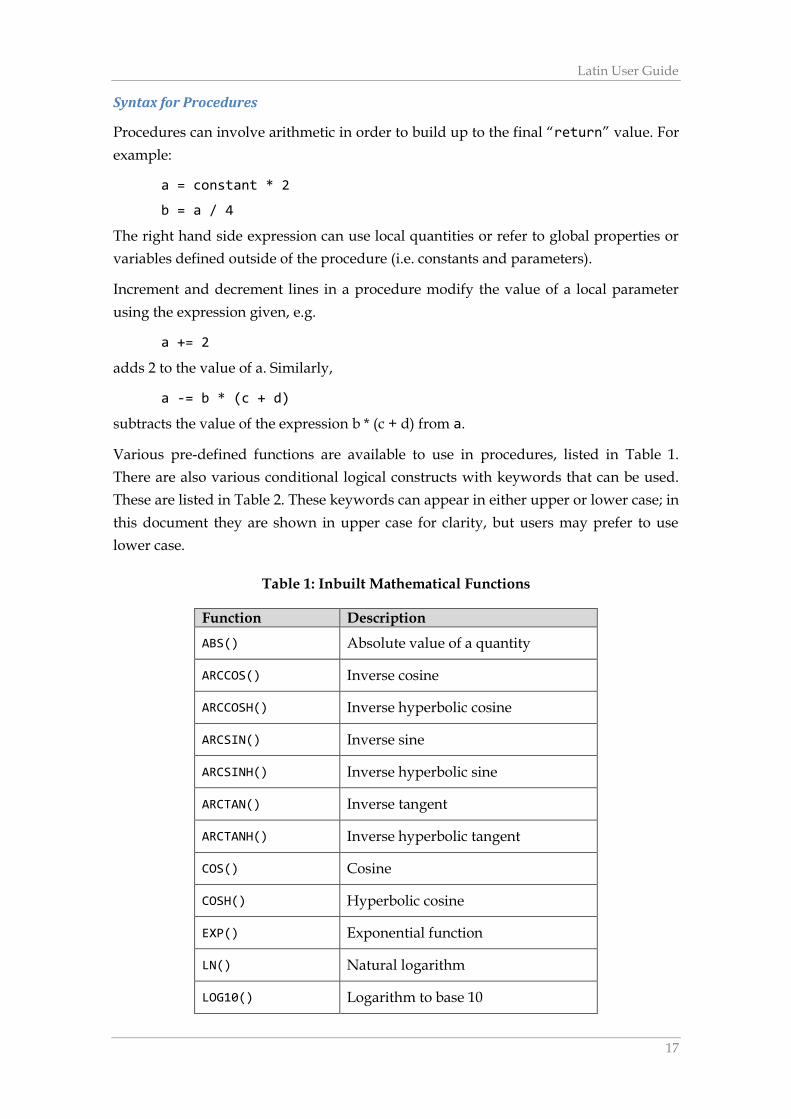
Various pre-defined functions are available to use in procedures, listed in Table 1.
There are also various conditional logical constructs with keywords that can be used.
These are listed in Table 2. These keywords can appear in either upper or lower case; in
this document they are shown in upper case for clarity, but users may prefer to use
lower case.
Table 1: Inbuilt Mathematical Functions
Function Description
ABS() Absolute value of a quantity
ARCCOS() Inverse cosine
ARCCOSH() Inverse hyperbolic cosine
ARCSIN() Inverse sine
ARCSINH() Inverse hyperbolic sine
ARCTAN() Inverse tangent
ARCTANH() Inverse hyperbolic tangent
COS() Cosine
COSH() Hyperbolic cosine
EXP() Exponential function
LN() Natural logarithm
LOG10() Logarithm to base 10
Latin User Guide, Version 1.0
18
Function Description
MIN() Minimum of a comma separated list
MAX() Maximum of a comma separated list
SIN() Sine
SINH() Hyperbolic sine
SQRT() Square root
TAN() Tangent
TANH() Hyperbolic tangent
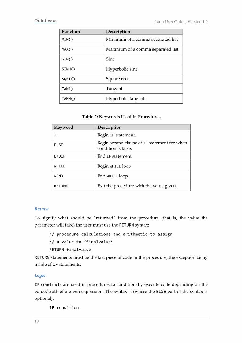
Table 2: Keywords Used in Procedures
Keyword Description
IF Begin IF statement.
ELSE Begin second clause of IF statement for when condition is false.
ENDIF End IF statement
WHILE Begin WHILE loop
WEND End WHILE loop
RETURN Exit the procedure with the value given.
Return
To signify what should be “returned” from the procedure (that is, the value the
parameter will take) the user must use the RETURN syntax:
// procedure calculations and arithmetic to assign
// a value to ‘finalvalue’
RETURN finalvalue
RETURN statements must be the last piece of code in the procedure, the exception being
inside of IF statements.
Logic
IF constructs are used in procedures to conditionally execute code depending on the
value/truth of a given expression. The syntax is (where the ELSE part of the syntax is
optional):
IF condition
Latin User Guide
19
// code to execute if expression is true
ELSE
// code to execute if expression is false
ENDIF
WHILE loops can be used in procedures to execute a block of code repeatedly while a
specific condition holds. The syntax is:
WHILE condition
// code to execute while statement is true
WEND
The conditions here can depend on local parameter values (those defined inside the
procedure) and global parameter values (those defined outside of the procedure). It
should not depend on time.
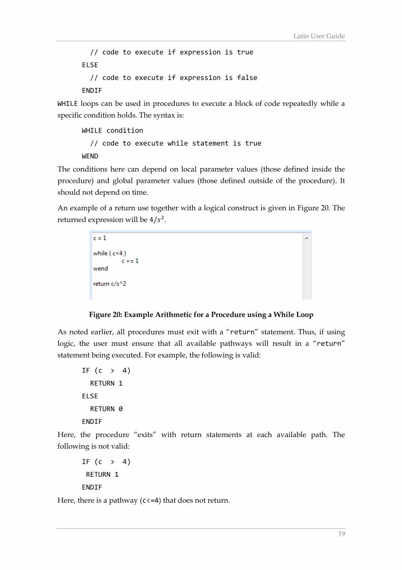
An example of a return use together with a logical construct is given in Figure 20. The
returned expression will be 4/𝑠2.
Figure 20: Example Arithmetic for a Procedure using a While Loop
As noted earlier, all procedures must exit with a “return” statement. Thus, if using
logic, the user must ensure that all available pathways will result in a “return”
statement being executed. For example, the following is valid:
IF (c > 4)
RETURN 1
ELSE
RETURN 0
ENDIF
Here, the procedure “exits” with return statements at each available path. The
following is not valid:
IF (c > 4)
RETURN 1
ENDIF
Here, there is a pathway (c<=4) that does not return.
Latin User Guide, Version 1.0
20
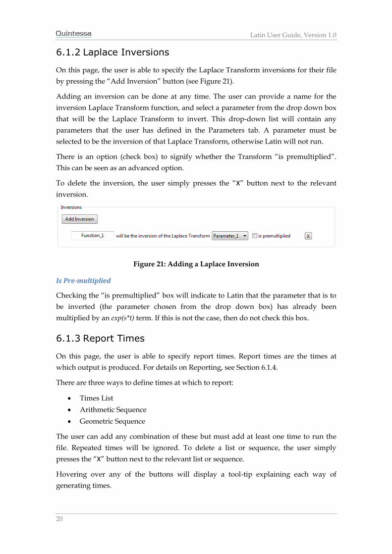
6.1.2 Laplace Inversions
On this page, the user is able to specify the Laplace Transform inversions for their file
by pressing the “Add Inversion” button (see Figure 21).
Adding an inversion can be done at any time. The user can provide a name for the
inversion Laplace Transform function, and select a parameter from the drop down box
that will be the Laplace Transform to invert. This drop-down list will contain any
parameters that the user has defined in the Parameters tab. A parameter must be
selected to be the inversion of that Laplace Transform, otherwise Latin will not run.
There is an option (check box) to signify whether the Transform “is premultiplied”.
This can be seen as an advanced option.
To delete the inversion, the user simply presses the “X” button next to the relevant
inversion.
Figure 21: Adding a Laplace Inversion
Is Pre-multiplied
Checking the “is premultiplied” box will indicate to Latin that the parameter that is to
be inverted (the parameter chosen from the drop down box) has already been
multiplied by an exp(s*t) term. If this is not the case, then do not check this box.
6.1.3 Report Times
On this page, the user is able to specify report times. Report times are the times at
which output is produced. For details on Reporting, see Section 6.1.4.
There are three ways to define times at which to report:
Times List
Arithmetic Sequence
Geometric Sequence
The user can add any combination of these but must add at least one time to run the
file. Repeated times will be ignored. To delete a list or sequence, the user simply
presses the “X” button next to the relevant list or sequence.
Hovering over any of the buttons will display a tool-tip explaining each way of
generating times.
Latin User Guide
21
When at least one valid time has been specified, pressing the “refresh” button next to
the ‘List of Report Times’ heading will generate a grid list of the currently
specified valid times. Any time that a sequence/list is changed or added, the user will
need to refresh the gird to see each individual time.
Times List
To add a times list, the user simply presses the “Add Times List” button (see Figure
22). This will display a long text box for the list of times together with a short text box
for the units. By default, the times 1 2 3 4 5 are given as an example. The list of times
should be space separated within the text box.
Figure 22: Adding a Times List
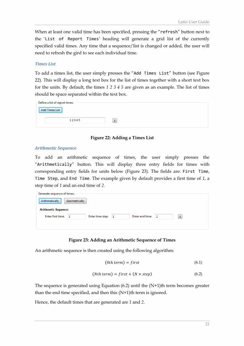
Arithmetic Sequence
To add an arithmetic sequence of times, the user simply presses the
“Arithmetically” button. This will display three entry fields for times with
corresponding entry fields for units below (Figure 23). The fields are: First Time,
Time Step, and End Time. The example given by default provides a first time of 1, a
step time of 1 and an end time of 2.
Figure 23: Adding an Arithmetic Sequence of Times
An arithmetic sequence is then created using the following algorithm:
(0𝑡ℎ 𝑡𝑒𝑟𝑚) = 𝑓𝑖𝑟𝑠𝑡 (6.1)
(𝑁𝑡ℎ 𝑡𝑒𝑟𝑚) = 𝑓𝑖𝑟𝑠𝑡 + (𝑁 × 𝑠𝑡𝑒𝑝) (6.2)
The sequence is generated using Equation (6.2) until the (N+1)th term becomes greater
than the end time specified, and then this (N+1)th term is ignored.
Hence, the default times that are generated are 1 and 2.
Latin User Guide, Version 1.0
22
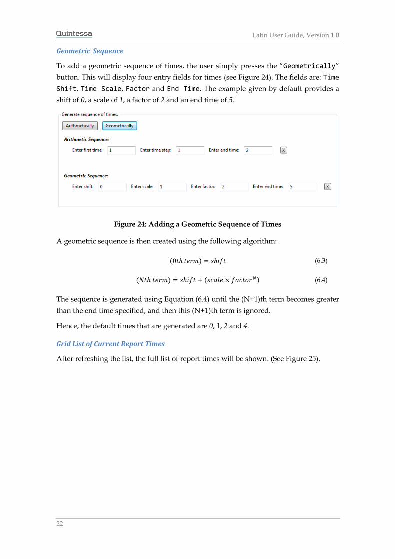
Geometric Sequence
To add a geometric sequence of times, the user simply presses the “Geometrically”
button. This will display four entry fields for times (see Figure 24). The fields are: Time
Shift, Time Scale, Factor and End Time. The example given by default provides a
shift of 0, a scale of 1, a factor of 2 and an end time of 5.
Figure 24: Adding a Geometric Sequence of Times
A geometric sequence is then created using the following algorithm:
(0𝑡ℎ 𝑡𝑒𝑟𝑚) = 𝑠ℎ𝑖𝑓𝑡 (6.3)
(𝑁𝑡ℎ 𝑡𝑒𝑟𝑚) = 𝑠ℎ𝑖𝑓𝑡 + (𝑠𝑐𝑎𝑙𝑒 × 𝑓𝑎𝑐𝑡𝑜𝑟𝑁) (6.4)
The sequence is generated using Equation (6.4) until the (N+1)th term becomes greater
than the end time specified, and then this (N+1)th term is ignored.
Hence, the default times that are generated are 0, 1, 2 and 4.
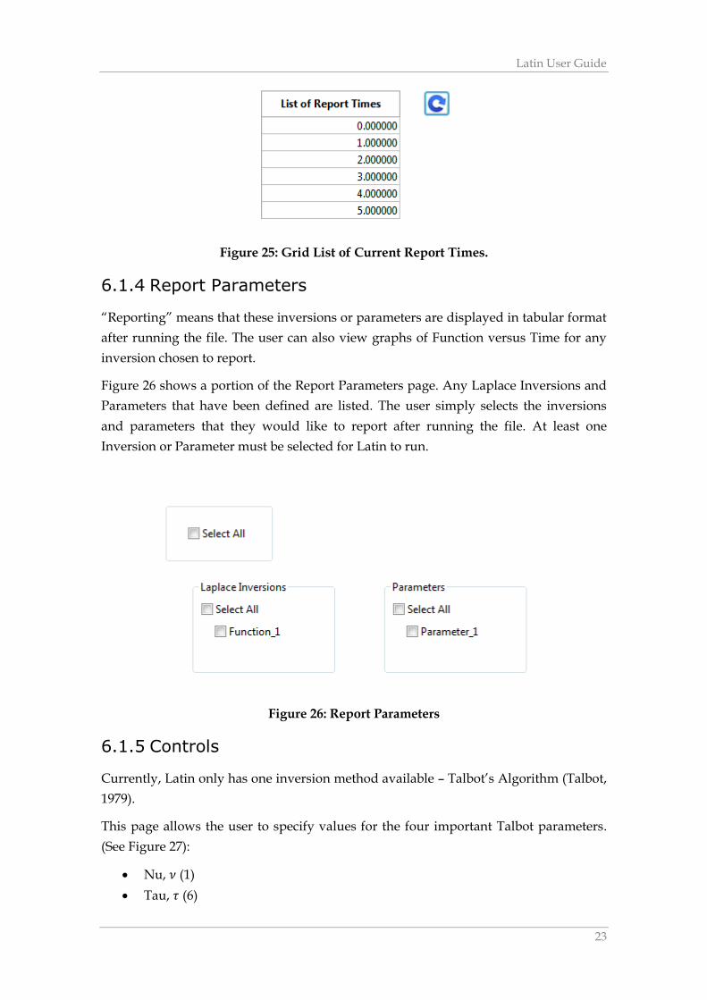
Grid List of Current Report Times
After refreshing the list, the full list of report times will be shown. (See Figure 25).
Latin User Guide
23
Figure 25: Grid List of Current Report Times.
6.1.4 Report Parameters
“Reporting” means that these inversions or parameters are displayed in tabular format
after running the file. The user can also view graphs of Function versus Time for any
inversion chosen to report.
Figure 26 shows a portion of the Report Parameters page. Any Laplace Inversions and
Parameters that have been defined are listed. The user simply selects the inversions
and parameters that they would like to report after running the file. At least one
Inversion or Parameter must be selected for Latin to run.
Figure 26: Report Parameters
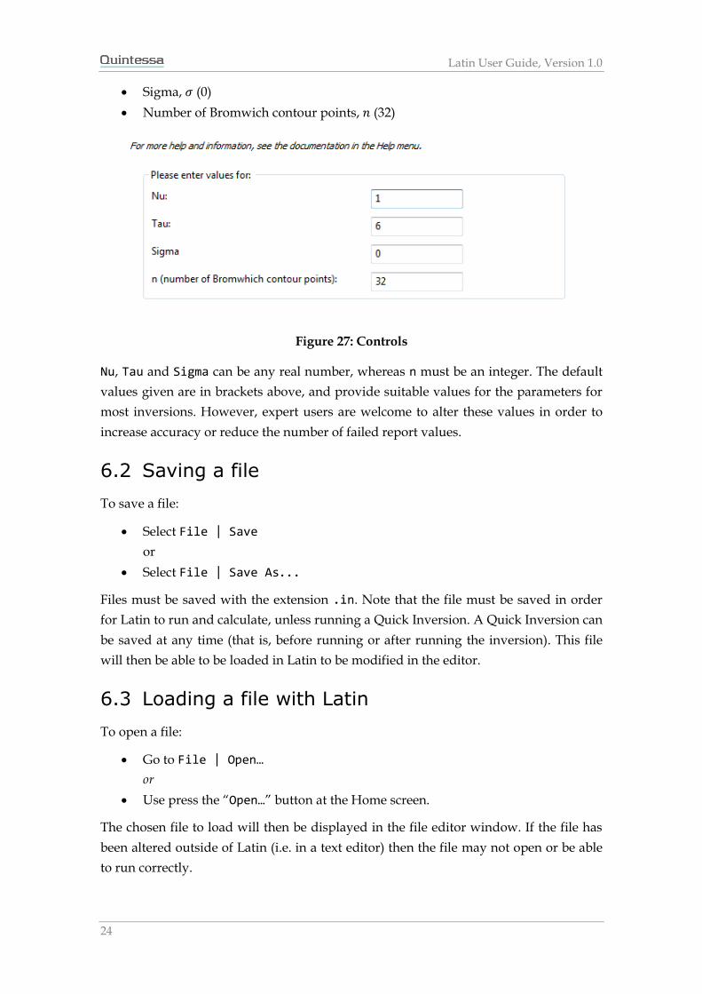
6.1.5 Controls
Currently, Latin only has one inversion method available – Talbot’s Algorithm (Talbot,
1979).
This page allows the user to specify values for the four important Talbot parameters.
(See Figure 27):
Nu, 𝜈 (1)
Tau, 𝜏 (6)
Latin User Guide, Version 1.0
24
Sigma, 𝜎 (0)
Number of Bromwich contour points, 𝑛 (32)
Figure 27: Controls
Nu, Tau and Sigma can be any real number, whereas n must be an integer. The default
values given are in brackets above, and provide suitable values for the parameters for
most inversions. However, expert users are welcome to alter these values in order to
increase accuracy or reduce the number of failed report values.
6.2 Saving a file
To save a file:
Select File | Save
or
Select File | Save As...
Files must be saved with the extension .in. Note that the file must be saved in order
for Latin to run and calculate, unless running a Quick Inversion. A Quick Inversion can
be saved at any time (that is, before running or after running the inversion). This file
will then be able to be loaded in Latin to be modified in the editor.
6.3 Loading a file with Latin
To open a file:
Go to File | Open…
or
Use press the “Open…” button at the Home screen.
The chosen file to load will then be displayed in the file editor window. If the file has
been altered outside of Latin (i.e. in a text editor) then the file may not open or be able
to run correctly.
Latin User Guide
25
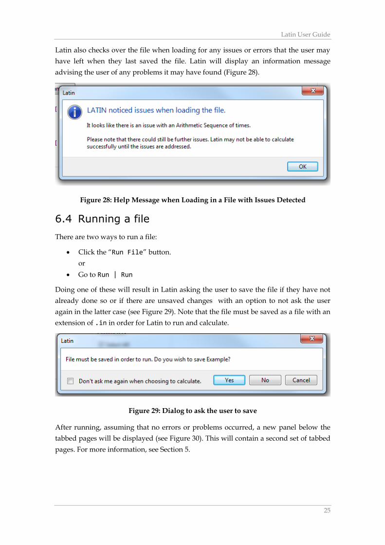
Latin also checks over the file when loading for any issues or errors that the user may
have left when they last saved the file. Latin will display an information message
advising the user of any problems it may have found (Figure 28).
Figure 28: Help Message when Loading in a File with Issues Detected
6.4 Running a file
There are two ways to run a file:
Click the “Run File” button.
or
Go to Run | Run
Doing one of these will result in Latin asking the user to save the file if they have not
already done so or if there are unsaved changes with an option to not ask the user
again in the latter case (see Figure 29). Note that the file must be saved as a file with an
extension of .in in order for Latin to run and calculate.
Figure 29: Dialog to ask the user to save
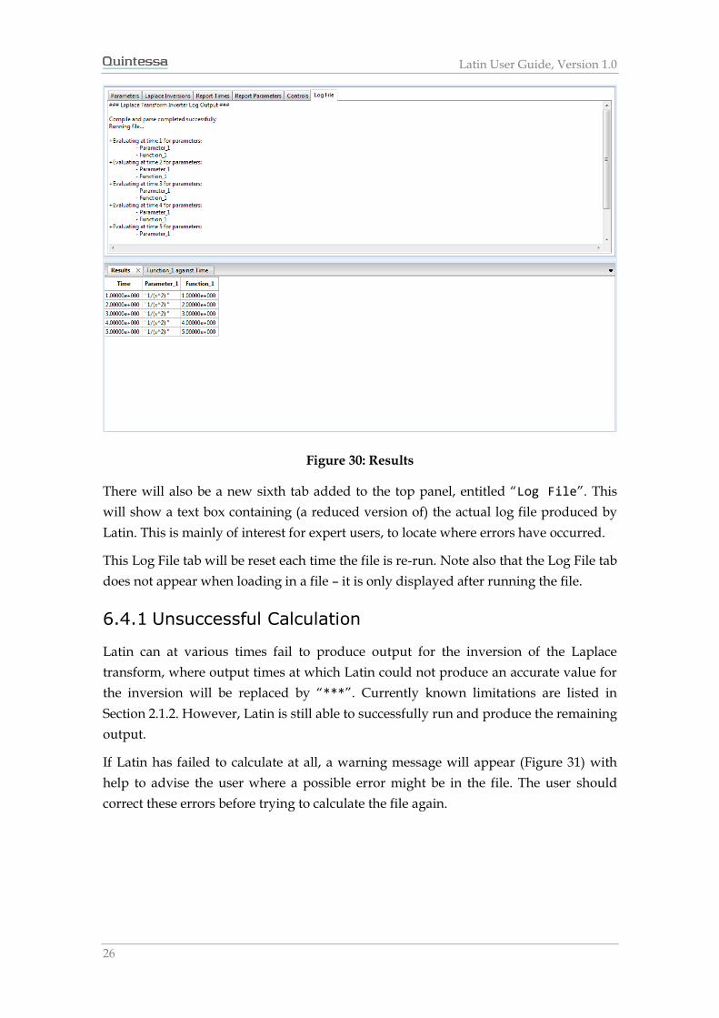
After running, assuming that no errors or problems occurred, a new panel below the
tabbed pages will be displayed (see Figure 30). This will contain a second set of tabbed
pages. For more information, see Section 5.
Latin User Guide, Version 1.0
26
Figure 30: Results
There will also be a new sixth tab added to the top panel, entitled “Log File”. This
will show a text box containing (a reduced version of) the actual log file produced by
Latin. This is mainly of interest for expert users, to locate where errors have occurred.
This Log File tab will be reset each time the file is re-run. Note also that the Log File tab
does not appear when loading in a file – it is only displayed after running the file.
6.4.1 Unsuccessful Calculation
Latin can at various times fail to produce output for the inversion of the Laplace
transform, where output times at which Latin could not produce an accurate value for
the inversion will be replaced by “***”. Currently known limitations are listed in
Section 2.1.2. However, Latin is still able to successfully run and produce the remaining
output.
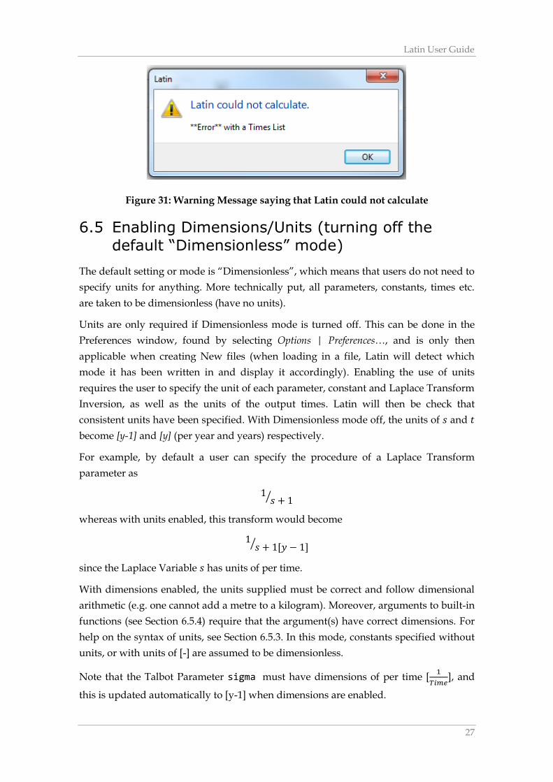
If Latin has failed to calculate at all, a warning message will appear (Figure 31) with
help to advise the user where a possible error might be in the file. The user should
correct these errors before trying to calculate the file again.
Latin User Guide
27
Figure 31: Warning Message saying that Latin could not calculate
6.5 Enabling Dimensions/Units (turning off the
default “Dimensionless” mode)
The default setting or mode is “Dimensionless”, which means that users do not need to
specify units for anything. More technically put, all parameters, constants, times etc.
are taken to be dimensionless (have no units).
Units are only required if Dimensionless mode is turned off. This can be done in the
Preferences window, found by selecting Options | Preferences…, and is only then
applicable when creating New files (when loading in a file, Latin will detect which
mode it has been written in and display it accordingly). Enabling the use of units
requires the user to specify the unit of each parameter, constant and Laplace Transform
Inversion, as well as the units of the output times. Latin will then be check that
consistent units have been specified. With Dimensionless mode off, the units of 𝑠 and 𝑡
become [y-1] and [y] (per year and years) respectively.
For example, by default a user can specify the procedure of a Laplace Transform
parameter as
1𝑠 + 1⁄
whereas with units enabled, this transform would become
1𝑠 + 1[𝑦 − 1]⁄
since the Laplace Variable 𝑠 has units of per time.
With dimensions enabled, the units supplied must be correct and follow dimensional
arithmetic (e.g. one cannot add a metre to a kilogram). Moreover, arguments to built-in
functions (see Section 6.5.4) require that the argument(s) have correct dimensions. For
help on the syntax of units, see Section 6.5.3. In this mode, constants specified without
units, or with units of [-] are assumed to be dimensionless.
Note that the Talbot Parameter sigma must have dimensions of per time [1
𝑇𝑖𝑚𝑒], and
this is updated automatically to [y-1] when dimensions are enabled.
Latin User Guide, Version 1.0
28
6.5.1 Laplace Transform Inversions with Units
As mentioned, the user will also have to specify units for the Inverse Laplace
Transform as well. As a guide, since a Laplace Transform of a function is an integral i.e.
ℒ{𝑓(𝑡)}(𝑠) = 𝐹(𝑠) = ∫ 𝑓(𝑡) exp(−𝑠𝑡) 𝑑𝑡∞
0,
𝑓(𝑡) must have dimensions of [{𝐷𝑖𝑚𝑒𝑠𝑛𝑖𝑜𝑛 𝑜𝑓 𝐹(𝑠)
𝑇] where [𝑇] represents the dimensions of
time.
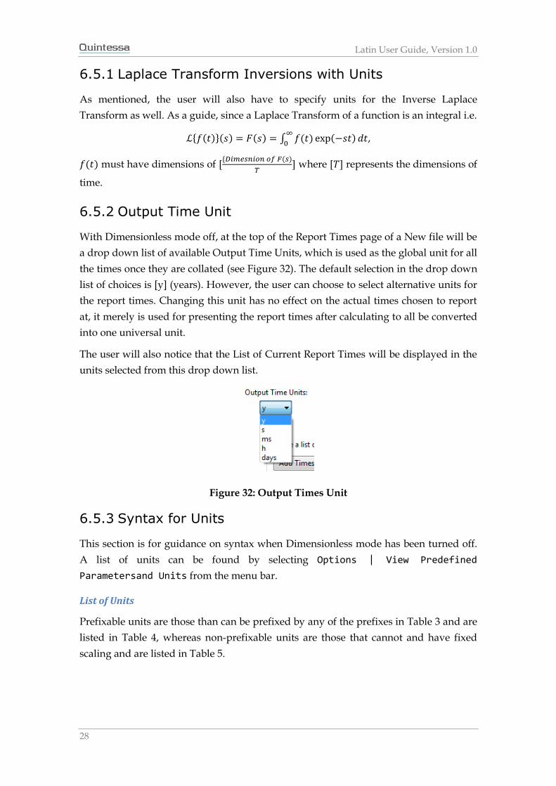
6.5.2 Output Time Unit
With Dimensionless mode off, at the top of the Report Times page of a New file will be
a drop down list of available Output Time Units, which is used as the global unit for all
the times once they are collated (see Figure 32). The default selection in the drop down
list of choices is [y] (years). However, the user can choose to select alternative units for
the report times. Changing this unit has no effect on the actual times chosen to report
at, it merely is used for presenting the report times after calculating to all be converted
into one universal unit.
The user will also notice that the List of Current Report Times will be displayed in the
units selected from this drop down list.
Figure 32: Output Times Unit
6.5.3 Syntax for Units
This section is for guidance on syntax when Dimensionless mode has been turned off.
A list of units can be found by selecting Options | View Predefined
Parametersand Units from the menu bar.
List of Units
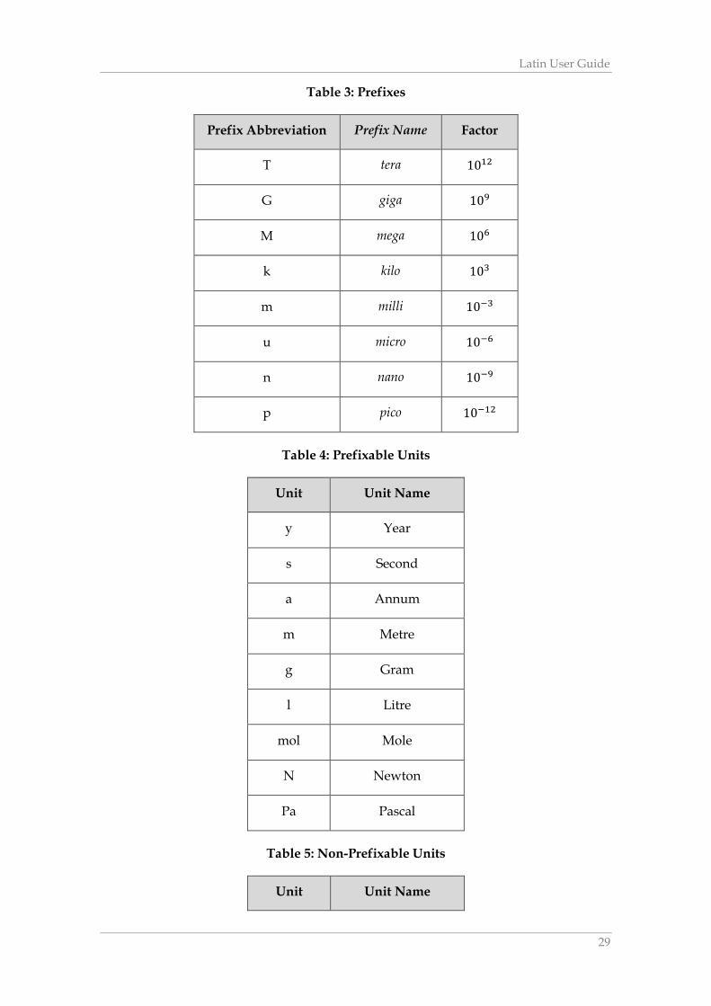
Prefixable units are those than can be prefixed by any of the prefixes in Table 3 and are
listed in Table 4, whereas non-prefixable units are those that cannot and have fixed
scaling and are listed in Table 5.
Latin User Guide
29
Table 3: Prefixes
Prefix Abbreviation Prefix Name Factor
T tera 1012
G giga 109
M mega 106
k kilo 103
m milli 10−3
u micro 10−6
n nano 10−9
p pico 10−12
Table 4: Prefixable Units
Unit Unit Name
y Year
s Second
a Annum
m Metre
g Gram
l Litre
mol Mole
N Newton
Pa Pascal
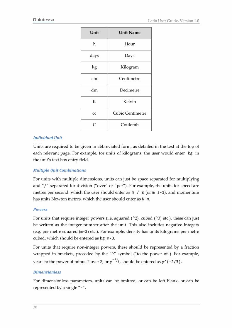
Table 5: Non-Prefixable Units
Unit Unit Name
Latin User Guide, Version 1.0
30
Unit Unit Name
h Hour
days Days
kg Kilogram
cm Centimetre
dm Decimetre
K Kelvin
cc Cubic Centimetre
C Coulomb
Individual Unit
Units are required to be given in abbreviated form, as detailed in the text at the top of
each relevant page. For example, for units of kilograms, the user would enter kg in
the unit’s text box entry field.
Multiple Unit Combinations
For units with multiple dimensions, units can just be space separated for multiplying
and “/” separated for division (“over” or “per”). For example, the units for speed are
metres per second, which the user should enter as m / s (or m s-1), and momentum
has units Newton metres, which the user should enter as N m.
Powers
For units that require integer powers (i.e. squared (^2), cubed (^3) etc.), these can just
be written as the integer number after the unit. This also includes negative integers
(e.g. per metre squared (m-2) etc.). For example, density has units kilograms per metre
cubed, which should be entered as kg m-3.
For units that require non-integer powers, these should be represented by a fraction
wrapped in brackets, preceded by the “^” symbol (“to the power of”). For example,
years to the power of minus 2 over 3, or 𝑦−2
3⁄ , should be entered as y^(-2/3).
Dimensionless
For dimensionless parameters, units can be omitted, or can be left blank, or can be
represented by a single “-“.
Latin User Guide
31
6.5.4 Parameter Procedures
Assignment lines in a procedure must have consistent units, and simply set the value
of a local parameter (defined in the procedure) to the expression given. For example:
a = b + 2 [m]
The units of local parameters are deduced when they are first used and subsequent
uses must be consistent with this.
The right hand side expression can use local quantities or refer to global properties or
variables (defined outside the procedure).
Increment and decrement lines in a procedure modify the value of a local parameter
using the expression given, e.g.
a += 2 [m]
adds 2 metres to the value of a. Similarly
a -= b * (c + d)
subtracts the value of the expression b * (c + d) from a, provided that the dimensions of
both sides of the equation are consistent.
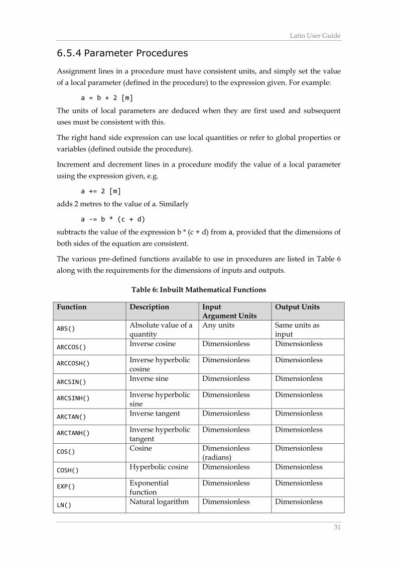
The various pre-defined functions available to use in procedures are listed in Table 6
along with the requirements for the dimensions of inputs and outputs.
Table 6: Inbuilt Mathematical Functions
Function Description Input Argument Units
Output Units
ABS() Absolute value of a quantity
Any units Same units as input
ARCCOS() Inverse cosine Dimensionless Dimensionless
ARCCOSH() Inverse hyperbolic cosine
Dimensionless Dimensionless
ARCSIN() Inverse sine Dimensionless Dimensionless
ARCSINH() Inverse hyperbolic sine
Dimensionless Dimensionless
ARCTAN() Inverse tangent Dimensionless Dimensionless
ARCTANH() Inverse hyperbolic tangent
Dimensionless Dimensionless
COS() Cosine Dimensionless (radians)
Dimensionless
COSH() Hyperbolic cosine Dimensionless Dimensionless
EXP() Exponential function
Dimensionless Dimensionless
LN() Natural logarithm Dimensionless Dimensionless
Latin User Guide, Version 1.0
32
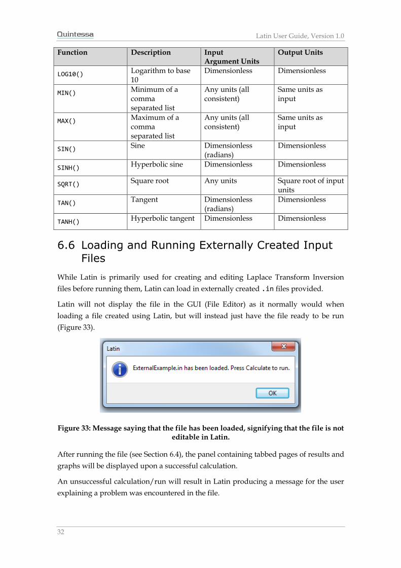
Function Description Input Argument Units
Output Units
LOG10() Logarithm to base 10
Dimensionless Dimensionless
MIN() Minimum of a comma separated list
Any units (all consistent)
Same units as input
MAX() Maximum of a comma separated list
Any units (all consistent)
Same units as input
SIN() Sine Dimensionless (radians)
Dimensionless
SINH() Hyperbolic sine Dimensionless Dimensionless
SQRT() Square root Any units Square root of input units
TAN() Tangent Dimensionless (radians)
Dimensionless
TANH() Hyperbolic tangent Dimensionless Dimensionless
6.6 Loading and Running Externally Created Input
Files
While Latin is primarily used for creating and editing Laplace Transform Inversion
files before running them, Latin can load in externally created .in files provided.
Latin will not display the file in the GUI (File Editor) as it normally would when
loading a file created using Latin, but will instead just have the file ready to be run
(Figure 33).
Figure 33: Message saying that the file has been loaded, signifying that the file is not editable in Latin.
After running the file (see Section 6.4), the panel containing tabbed pages of results and
graphs will be displayed upon a successful calculation.
An unsuccessful calculation/run will result in Latin producing a message for the user
explaining a problem was encountered in the file.
Latin User Guide
33
6.7 Output files
Once a file has been run, certain output files are produced in the same directory of the
input file. These are:
A log file – named filename.log
A CSV (comma separated values) results file – named filename_results.csv
These files can be ignored, however some users may find the contents useful.
The log file can be opened in any text editor (like Notepad) and contains information
about how the file was parsed before calculating, and contains any messages regarding
issues and errors that the solver produces.
The CSV file can be opened in programs like Microsoft Excel, and contains the same
information stored in the Results Table from Section 5.1.1.
References
Robinson P and Maul P (1991) Some experience with the numerical inversion of
Laplace transforms, Math. Engng. Ind., Vol. 3, No. 2, pp. 111-131
Rondini (2007) wxMathPlot: Scientific plotting for wxWidgets website
http://wxmathplot.sourceforge.net/index.shtml
Talbot A (1979) The Accurate Numerical Inversion of Laplace Transforms. J. Inst. Math.
Appl. 23.