Embed Size (px)
Citation preview

Johannes Stoerkle
Lateral Dynamics ofMultiaxle Vehicles
Master Thesis
Institute for Dynamic Systems and ControlSwiss Federal Institute of Technology (ETH) Zurich
Supervision
M. Alberding (ETH Zurich)Prof. Dr. L. Guzzella (ETH Zurich)
Prof. Dr. W. Schiehlen (University of Stuttgart)Prof. Dr. P. Eberhard (University of Stuttgart)
– THE CONFIDENTIAL CONTENT IS RESTRICTED –
July 2013
IDSC-LG-MA-05


Diploma Thesis DIPL-MSC-196
Lateral Dynamics of
Multiaxle Vehicles
of
Johannes Stoerkle
Betreuer: M. Alberding (ETH Zurich)Prof. Dr. L. Guzzella (ETH Zurich)Prof. Dr. W. Schiehlen (University of Stuttgart)Prof. Dr. P. Eberhard (University of Stuttgart)
– THE CONFIDENTIAL CONTENT IS RESTRICTED –
University of StuttgartInstitute of Engineering and Computational Mechanics
Prof. Dr.–Ing. Prof. E.h. P. Eberhard
July 2013


Abstract
Since standard European semitrailers usually utilize an unsteered rear tri-axle group they areproduced with low financial efforts but have a high tire wear (especially at the rearmost axle)and a reduced maneuverability. This work shows that an actively steered rearmost axle at asemitrailer can improve the performance during low-speed turning maneuvers, high-speed corneringand could intervene during critical situations such as rollover. After some general fundamentals ofvehicle dynamics are summarized, the current state of art with respect to steered semitrailers isdiscussed. Linear and nonlinear tractor-semitrailer single-track models are derived, which take thelateral and yaw motion of the coupled vehicles into account and can be used for the developmentof different steering strategies for an enhanced maneuverability. In this scope a steady-state andfeedback control strategy is developed. In addition, a 2-degree of freedom controller combines bothstrategies. Furthermore, the models are extended in order to account for the roll motions of thesystem at high-speed. A simple “active rollover damping control law” is proposed and investigated,which intervenes with the trailer steering and aims to reduce the risk of a rollover. In conclusion, the2-degree of freedom control law improves the maneuverability of a whole tractor-semitrailer systemand the active rollover damping strategy decreases the risk of a rollover significantly during criticalmaneuvers. The derived models and strategies provide different chances for further optimizations,improvments and implementations on real tractor-semitrailer prototypes.
i

Contents
Contents ii
1 Introduction 11.1 Motivation . . . . . . . . . . . . . . . . . . . . . . . . . . . . . . . . . . . . . . . . . 11.2 Structure and Scope . . . . . . . . . . . . . . . . . . . . . . . . . . . . . . . . . . . . 3
2 Fundamentals and State of the Art 52.1 Basics of Vehicle Dynamics . . . . . . . . . . . . . . . . . . . . . . . . . . . . . . . . 5
2.1.1 Tire Mechanics . . . . . . . . . . . . . . . . . . . . . . . . . . . . . . . . . . . 52.1.2 Bicycle Model . . . . . . . . . . . . . . . . . . . . . . . . . . . . . . . . . . . . 72.1.3 Multiple Non-Steered Axles . . . . . . . . . . . . . . . . . . . . . . . . . . . . 112.1.4 Trailer Combinations . . . . . . . . . . . . . . . . . . . . . . . . . . . . . . . . 13
2.2 State of the Art: Steering of Semitrailer’s Rearmost Axle . . . . . . . . . . . . . . . 152.2.1 Horizontal Tracking Control Strategies . . . . . . . . . . . . . . . . . . . . . . 152.2.2 Rollover Prevention Control . . . . . . . . . . . . . . . . . . . . . . . . . . . . 17
2.3 Basics of Applied Mechanics and System Dynamics . . . . . . . . . . . . . . . . . . . 17
3 Modelling 193.1 Nonlinear Single-Track Model . . . . . . . . . . . . . . . . . . . . . . . . . . . . . . . 19
3.1.1 Equations of motion according to the Newton-Euler Approach . . . . . . . . 203.1.2 Transformation to trailer-fixed reference frame . . . . . . . . . . . . . . . . . 22
3.2 Model Extensions and Background Analysis . . . . . . . . . . . . . . . . . . . . . . . 243.2.1 Trajectories with respect to the Initial Reference Frame . . . . . . . . . . . . 243.2.2 Tire Forces and Kinematic Constraints . . . . . . . . . . . . . . . . . . . . . . 25
3.3 Linear Single-Track Model . . . . . . . . . . . . . . . . . . . . . . . . . . . . . . . . . 293.3.1 Fully Linear Equations of Motions . . . . . . . . . . . . . . . . . . . . . . . . 303.3.2 Linear Equations of Motion with saturated Tire Forces . . . . . . . . . . . . . 32
3.4 Roll-extended Single-Track Models . . . . . . . . . . . . . . . . . . . . . . . . . . . . 323.4.1 Nonlinear Lateral-Yaw-Roll Model . . . . . . . . . . . . . . . . . . . . . . . . 323.4.2 Linear Lateral-Yaw-Roll Model . . . . . . . . . . . . . . . . . . . . . . . . . . 353.4.3 Load Transfer Ratio (LTR) . . . . . . . . . . . . . . . . . . . . . . . . . . . . 37
3.5 SimPack Model . . . . . . . . . . . . . . . . . . . . . . . . . . . . . . . . . . . . . . . 40
4 Control Strategies 414.1 Virtual Driver . . . . . . . . . . . . . . . . . . . . . . . . . . . . . . . . . . . . . . . . 41
4.1.1 Cruise Control . . . . . . . . . . . . . . . . . . . . . . . . . . . . . . . . . . . 414.1.2 Tractors Steering Control . . . . . . . . . . . . . . . . . . . . . . . . . . . . . 42
4.2 Steering Strategies for the Track-Tracing of a Semitrailer . . . . . . . . . . . . . . . . 444.2.1 Feedforward Controller for a Steady-State Turn . . . . . . . . . . . . . . . . . 444.2.2 Feed-Back Controller for a Path-Following . . . . . . . . . . . . . . . . . . . . 454.2.3 Feedforward-Feedback Control (FFFB) . . . . . . . . . . . . . . . . . . . . . 45
ii

4.2.4 FFFB with Reset & Patch-Strategy . . . . . . . . . . . . . . . . . . . . . . . 454.2.5 FFFB with Reset & Shift-Strategy . . . . . . . . . . . . . . . . . . . . . . . . 454.2.6 FFFB with Relative Coordinates . . . . . . . . . . . . . . . . . . . . . . . . . 45
4.3 Steering Strategies for Active Rollover Avoidance . . . . . . . . . . . . . . . . . . . . 454.3.1 Rollover of a Single-Unit Vehicle . . . . . . . . . . . . . . . . . . . . . . . . . 454.3.2 Active Roll Damping of a Tractor-Semitrailer . . . . . . . . . . . . . . . . . . 45
5 Simulation 475.1 Simulation Structure . . . . . . . . . . . . . . . . . . . . . . . . . . . . . . . . . . . . 47
5.1.1 Global Process Chain . . . . . . . . . . . . . . . . . . . . . . . . . . . . . . . 475.1.2 Structure of the Simulation Models . . . . . . . . . . . . . . . . . . . . . . . . 47
5.2 Results and Analysis . . . . . . . . . . . . . . . . . . . . . . . . . . . . . . . . . . . . 495.2.1 Response Characteristics of the linear Models . . . . . . . . . . . . . . . . . . 495.2.2 Validation of the TST-Models . . . . . . . . . . . . . . . . . . . . . . . . . . . 505.2.3 Track-Following Analysis with the Horizontal Planar Models . . . . . . . . . 525.2.4 Active-Roll-Damping Analysis with the Roll-extended Models . . . . . . . . . 52
5.3 Figures . . . . . . . . . . . . . . . . . . . . . . . . . . . . . . . . . . . . . . . . . . . 52
6 Summary and Outlook 57
A Model Parameters and Additional Derivations 59A.1 Vehicle Parameters . . . . . . . . . . . . . . . . . . . . . . . . . . . . . . . . . . . . . 59A.2 Math Notations . . . . . . . . . . . . . . . . . . . . . . . . . . . . . . . . . . . . . . . 59A.3 Equations of Motion according to the Lagrangian Approach . . . . . . . . . . . . . . 59A.4 Validation with the Bicycle Model . . . . . . . . . . . . . . . . . . . . . . . . . . . . 62A.5 Alternative Derivation of the linear TST Model . . . . . . . . . . . . . . . . . . . . . 64A.6 Symbolic derivation of the equations of motion using MATLAB . . . . . . . . . . . . 67
B Vehicle Animation with MatCarAnim 72
List of Figures 75
Bibliography 78

Chapter 1
Introduction
1.1 Motivation
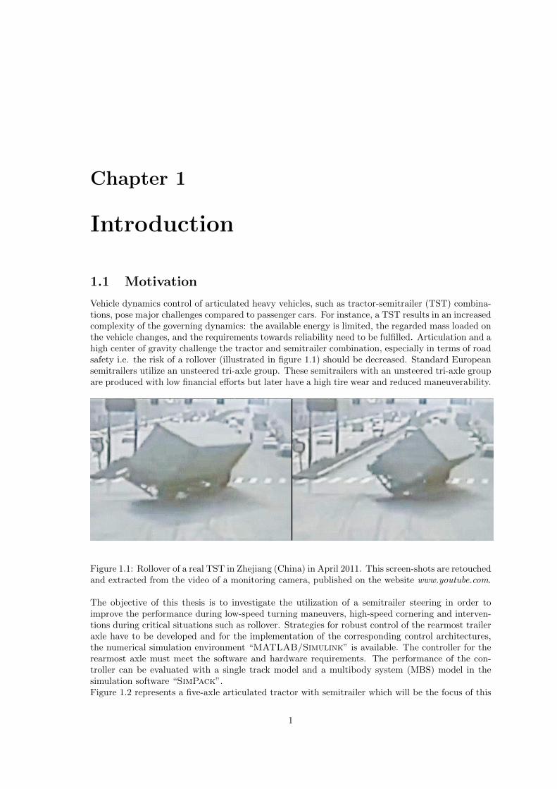
Vehicle dynamics control of articulated heavy vehicles, such as tractor-semitrailer (TST) combina-tions, pose major challenges compared to passenger cars. For instance, a TST results in an increasedcomplexity of the governing dynamics: the available energy is limited, the regarded mass loaded onthe vehicle changes, and the requirements towards reliability need to be fulfilled. Articulation and ahigh center of gravity challenge the tractor and semitrailer combination, especially in terms of roadsafety i.e. the risk of a rollover (illustrated in figure 1.1) should be decreased. Standard Europeansemitrailers utilize an unsteered tri-axle group. These semitrailers with an unsteered tri-axle groupare produced with low financial efforts but later have a high tire wear and reduced maneuverability.
Figure 1.1: Rollover of a real TST in Zhejiang (China) in April 2011. This screen-shots are retouchedand extracted from the video of a monitoring camera, published on the website www.youtube.com.
The objective of this thesis is to investigate the utilization of a semitrailer steering in order toimprove the performance during low-speed turning maneuvers, high-speed cornering and interven-tions during critical situations such as rollover. Strategies for robust control of the rearmost traileraxle have to be developed and for the implementation of the corresponding control architectures,the numerical simulation environment “MATLAB/Simulink” is available. The controller for therearmost axle must meet the software and hardware requirements. The performance of the con-troller can be evaluated with a single track model and a multibody system (MBS) model in thesimulation software “SimPack”.Figure 1.2 represents a five-axle articulated tractor with semitrailer which will be the focus of this
1
2 1.1. Motivation
TractorSemitrailer
5th-WheelActive Steered Rearmost Axle
Human Driver
Human Steered Front AxleHitch
Additional Cargo
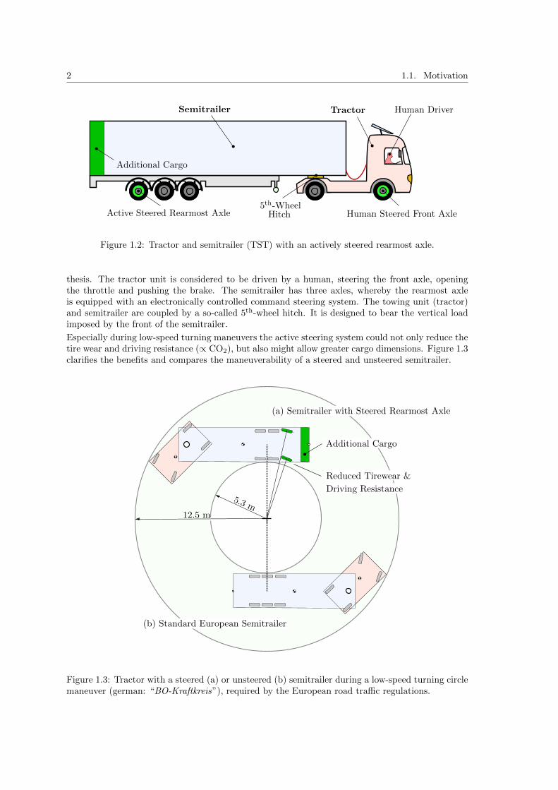
Figure 1.2: Tractor and semitrailer (TST) with an actively steered rearmost axle.
thesis. The tractor unit is considered to be driven by a human, steering the front axle, openingthe throttle and pushing the brake. The semitrailer has three axles, whereby the rearmost axleis equipped with an electronically controlled command steering system. The towing unit (tractor)and semitrailer are coupled by a so-called 5th-wheel hitch. It is designed to bear the vertical loadimposed by the front of the semitrailer.
Especially during low-speed turning maneuvers the active steering system could not only reduce thetire wear and driving resistance (∝ CO2), but also might allow greater cargo dimensions. Figure 1.3clarifies the benefits and compares the maneuverability of a steered and unsteered semitrailer.
12.5 m
5.3 m
(b) Standard European Semitrailer
(a) Semitrailer with Steered Rearmost Axle
Additional Cargo
Reduced Tirewear &
Driving Resistance
Figure 1.3: Tractor with a steered (a) or unsteered (b) semitrailer during a low-speed turning circlemaneuver (german: “BO-Kraftkreis”), required by the European road traffic regulations.

Chapter 1. Introduction 3
Since the steered axle improves the maneuverability, the semitrailer can be increased and additionalcargo can be transported. This leads to a higher efficiency, saves costs and resources.
1.2 Structure and Scope
This thesis is structured as follows:
• Chapter 2 Introduction of fundamentals of vehicle dynamics with respect to the characteri-zation of the tires, basic vehicle modeling and TST specific approaches. Furthermore, insightsof previous research are given.
• Chapter 3 Derivation of a linear and nonlinear horizontal TST model to describe the lateralvehicle dynamics at low-speed. In addition, the derived models will be extended in order toaccount for the roll motions of the system at high-speed. Finally, an existing SimPack modelwill be introduced.
• Chapter 4 Development of control strategies for the tractor front axle steering and thesemitrailer rearmost axle steering. A controller will be proposed, which aims to reduce therisk of a trailer rollover.
• Chapter 5 Implementation of the derived models and controllers in the simulation envi-ronments. The influences and improvements of the steering strategies will be investigated,analyzing the simulation results of the horizontal and vertical roll-extended models duringcertain maneuvers.
• Chapter 6 Summary of main aspects are given, including conclusion and future researchtopics.

4 1.2. Structure and Scope

Chapter 2
Fundamentals and State of the Art
2.1 Basics of Vehicle Dynamics
This chapter is meant to serve as an introduction to ground vehicle dynamics in order to presentthe characteristics of tires, development of vehicle models and explaining related technical terms.The focus is laid on the description of lateral dynamics during cornering at low and high velocity.
2.1.1 Tire Mechanics
The performance of a ground vehicle is mainly influenced by the tires. The tires interact betweenthe road and the vehicle and their properties are important for the dynamic behavior. This sectionbriefly gives the basic aspects of the force and moment generating properties of a pneumatic tire.Normal and friction forces are transmitted at the point of contact between a tire and the roadsurface. In figure 2.1 the SAE-standard for axis system [SAE76] is shown. The tire is centered inthe wheel plane perpendicular to the axis of rotation. Since it moves with the velocity v in the
x
v
z
y
Ω
γ
α
Wheelplane
inclination
slip
Direction ofwheel heading
Direction ofwheel travel
Spin axis
Angular velocity
Mx
My
Mz
Normal force (Fz)
Lateral force (Fy)
v
Rolling resistance
Overturning moment
Aligning
torque
Longitudialforce (Fx)
Figure 2.1: Tire axis system and terminology according to SAE-standards [SAE76].
5

6 2.1. Basics of Vehicle Dynamics
Fy
Fy
(b) Tire deformation in y-direction(a) Tire deformation on ground surface
Direction ofwheel heading Direction of
wheel travelα
contact patch
FyMz
slip
Figure 2.2: Origin of lateral forces.
direction of travel, side slip occurs. The lateral component of the slip is described by the tire sideslip angle α which effects a lateral force Fy. Because of this slip angle, the material in the contactpatch of the elastic tire is drifting to the side, explained in [Gil92] and illustrated in figure 2.2 (a).The deformation of the tire is also indicated in the cross-sectional view of figure 2.2 (b). Since thisthesis mainly considers simplified tire behavior of trucks in planar motions, the inclination of thewheels can be neglected. Full details about tire dynamics like e.g. the force and stress distributionat the contact patch are discussed in [Jaz09].Different tire models are proposed for the calculation of the lateral force during a simulation inthe literature of vehicle dynamics. One of the most common tire models is defined by the so-called“magic formula” in [Pac02]. According to this formula, the lateral force Fy can be calculated independency of the slip angle α and vertical force Fz,
Fy = D sin [arctanBα− E(Bα− arctan(Bα))] (2.1)
with the stiffness factor B =CαCD
, (2.2)
the peak factor D = µFz, (2.3)
and cornering stiffness Cα = c1 sin(2 arctan
(Fzc2
)) (SAE: Cα < 0). (2.4)
The shape factors C and E as well as the parameters c1 and c2 together with the friction coefficient µare depending on the tire material and design. They can be determined by experiments or empiricalvalues from the literature. The lateral force obtained by the ”magic formula” is schematically shownin figure 2.3 with respect to the slip angle. The relation is linear for small slip angles and can beapproximated by the function
Fy,lin(α) = Cα α (SAE: Cα < 0). (2.5)
As proposed in [Viv12] a saturated tire-force-law can be used in order to characterize the forcebehavior for larger slip angles,
Fy,sat(α) =
Cα α for |α| < αsat
Fy,max else, where Cα < 0. (2.6)

Chapter 2. Fundamentals and State of the Art 7
linear approximation
linear-saturated
”magic formula”
Lateral force Fy
slip angle α
approximation
CFα
Figure 2.3: Approximation of the lateral force in dependence of the slip angle according to Pacejka’stire model [Pac02] (SAE: Cα < 0).
The approximated tire-law also prevents the transgression of the linear range, which may causeexcessive lateral forces during a simulation process.
2.1.2 Bicycle Model
This section intends to introduce a simplified model of a four-wheeled vehicle with Ackermannsteering according to Riekert and Schunck (1940). Their linear theories of vehicle modeling hasalso been published by e.g. [Zom83]. As the two wheels on each axle are modeled by a centeredsubstitute wheel, their models are also known as ”bicycle models” or ”single-track models”. Thesubstitute wheel represents the tire and suspension characteristics of the related axle. Figure 2.4displays the so-called bicycle model during a steady state cornering of the vehicle at low velocity.The distance between the steered wheels of the front axle is defined by w, and the distance of
β0
lr
lf
c.g.
δ
i.c.r.
vr
v
vf
β0
δ
Ω0
Rr0
δi δo
w
Inner wheel Outer wheel
Rcg0
Figure 2.4: Conception of a single-track-model (Bicycle Model) based on an Ackermann steering.

8 2.1. Basics of Vehicle Dynamics
the center of gravity (c.g.) to the front axle respectively to the rear axle is denoted by lf and lr.The center of the reared axle moves with the velocity vr along a circle track with the radius Rr0.So the vehicle is turning with a constant angular velocity Ω0 around the instantaneous center ofrotation (i.c.r.). In analogy, the c.g. and the center of the front axle are moving with v and vf . Withthe assumption of low velocity, the centrifugal force can be neglected which leads to the followinggeometric conditions for the inner and outer steer angles
tan δi =l
Rr0 − w2
tan δo =l
Rr0 + w2
(2.7)
⇒ cot δo − cot δi =w
l. (2.8)
This is called the Ackermann condition, where l = lr+lf describes the wheelbase. The steer angle δof the single track model relates to the geometric lengths with
tan δ =l
Rr0. (2.9)
This equation can be used to eliminate the radius Rr0 in (2.7),
cot δi = cot δ − w
2lcot δo = cot δ +
w
2l. (2.10)
The bicycle steer angle is the cot-average of the inner and outer steer angles of the four-wheeledvehicle
cot δ =cot δo + cot δi
2, (2.11)
as it is also derived in [Jaz09]. Including the equation (2.9) it can be shown that the mass centerof the vehicle turns with the radius
Rcg0 =√l2r + l2 cot2 δ (2.12)
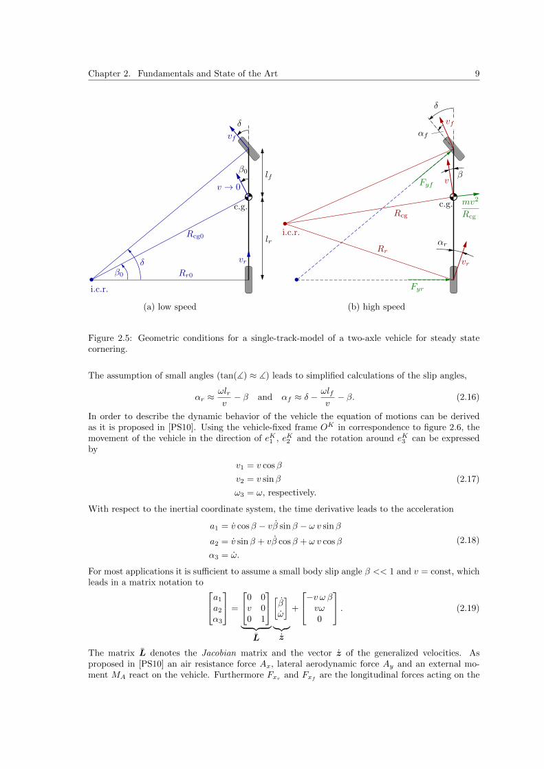
on the circle. The introduced relations are only valid for a small steady state cornering velocity v,as already mentioned.In case of the steady state cornering at high velocity, lateral accelerations must be taken intoaccount. In order to react against the centrifugal forces the tires develop the slip angles causinglateral forces. Figure 2.5 shows the difference between steady state cornering of a bicycle model atlow (a) and high (b) velocity. Due to the slip, the position of the i.c.r changes in dependency of thevehicle and the road conditions. According to the equation (2.5), the front and rear tire forces Fyfand Fyr are linear related to the front and rear slip angles αf and αr with
Fyf = Cαf αf and Fyr = Cαr αr, (2.13)
whereby Cαf and Cαr are the effective cornering stiffness at the front and rear axle. For thedetermination of the slip angles, it is necessary to consider the explicit wheel velocities more detailedas shown in figure 2.6. Since the vehicle is turning with the angular velocity (or yaw angularvelocity) ω around the c.g. and for a small body slip (β << 1), the rear and front wheel velocitiescan be approximately calculated with
vr ≈√v2 + (ωlr)2 and vf ≈
√v2 + (ωlf )2, (2.14)
where the absolute velocity of the vehicle is denoted by v. Furthermore, the following relationshipscan be derived for the body slip angle β,
tan(αr + β) ≈ ωlrv
and tan(δ − αf − β) ≈ ωlfv
. (2.15)
Chapter 2. Fundamentals and State of the Art 9
β0
lr
lf
c.g.
δ
i.c.r.
vr
v → 0
vf
β0
δ
β
c.g.
δ
i.c.r.
vr
v
vfαf
αr
(a) low speed (b) high speed
Rcg0
Rcg
Rr
Rr0
mv2
Rcg
Fyr
Fyf
Figure 2.5: Geometric conditions for a single-track-model of a two-axle vehicle for steady statecornering.
The assumption of small angles (tan(]) ≈ ]) leads to simplified calculations of the slip angles,
αr ≈ωlrv− β and αf ≈ δ −
ωlfv− β. (2.16)
In order to describe the dynamic behavior of the vehicle the equation of motions can be derivedas it is proposed in [PS10]. Using the vehicle-fixed frame OK in correspondence to figure 2.6, themovement of the vehicle in the direction of eK1 , eK2 and the rotation around eK3 can be expressedby
v1 = v cosβ
v2 = v sinβ
ω3 = ω, respectively.
(2.17)
With respect to the inertial coordinate system, the time derivative leads to the acceleration
a1 = v cosβ − vβ sinβ − ω v sinβ
a2 = v sinβ + vβ cosβ + ω v cosβ
α3 = ω.
(2.18)
For most applications it is sufficient to assume a small body slip angle β << 1 and v = const, whichleads in a matrix notation to a1
a2
α3
=
0 0v 00 1
︸ ︷︷ ︸L
[βω
]︸︷︷︸z
+
−v ω βvω0
. (2.19)
The matrix L denotes the Jacobian matrix and the vector z of the generalized velocities. Asproposed in [PS10] an air resistance force Ax, lateral aerodynamic force Ay and an external mo-ment MA react on the vehicle. Furthermore Fxr and Fxf are the longitudinal forces acting on the

10 2.1. Basics of Vehicle Dynamics
β
m , I
δ
i.c.r.
vr
v
vf
αf
αr
Rcg
Rr
mv2
Rcg
Fyr
Fyf
π2 − αr
π2 − β
αr + β
δ − αf− β
δ − αf + αrω
v
ωlr
ωlr
ωlf
v
ωlf
eK1eK2
OK
Fxr
Fxf
Ax
AyMA
Figure 2.6: Single-track-model of a two-axle vehicle at high velocity.
tires in the direction of the wheel heading. Neglecting small quadratically terms, the Newton-Eulerequations for the vehicle with the mass m and moment of inertia I results in 0 0
mv 00 I
[βω
]+
−mv ω βmvω0
=
Fxf + Fxr −Ax−Fyf − Fyr +AyFyrlr − Fyf lf +MA
. (2.20)
Applying the Jourdain’s principle, the equations of motion followed by a left multiplication with
the transposed Jacobian matrix LT
,[mv2 0
0 I
] [βω
]+
[mv2ω
0
] [v(−Fyf − Fyr +Ay)Fyrlr − Fyf lf +MA
]. (2.21)
With the linear tire model from (2.13), it leads to[mv2 0
0 I
] [βω
]+
[mv2ω
0
]=
[v(−Cαf αf − Cαr αr +Ay)Cαr αr lr − Cαf αf lf +MA
]. (2.22)
Using (2.16) it yields the Riekert and Schunck’s equations, also mentioned in [Zom83],
mvβ − (Cαf + Cαr)β +
(mv − lfCαf − lrCαr
v
)ω = Ay − Cαf δ (2.23)
Iω − 1
v(Cαr l
2r + Cαf l
2f )ω − (Cαf lf − Cαr lr)β = Ma − Cαf δ lf . (2.24)

Chapter 2. Fundamentals and State of the Art 11
Condition Case Required Driver Intervention
|Cαr| lr > |Cαf | lf understeering increasing required
|Cαr| lr = |Cαf | lf neutral steering -
|Cαr| lr < |Cαf | lf oversteering decreasing required
Table 2.1: Cases of vehicle steer behavior
Remark 2.1. The sign of the cornering stiffness differs, since the SAE-terminology is used in thiswork.
The derived equations can also be used to explain the oversteer and understeer phenomena. Inconsideration of a steady-state cornering (β = 0) and with the neglection of the aerodynamicforce (Ay = 0), the equation (2.23) can be rearranged to
δ =lω
v
(1 +
Cαf lf − CαrlrCαfCαrl2
mv2
), where Cαf , Cαr < 0. (2.25)
This means that the driver has to steer in relation to the velocity and the cornering stiffness ofthe front and rear axle in order to follow a constant cornering path. The steering behavior can besummarized with the cases specified in table 2.1.
2.1.3 Multiple Non-Steered Axles
Non-steered multiple-axle suspensions are typically used to sustain the weighty cargo, especiallywithin the scope of heavy vehicles. The two- and three-axle varieties are the most common types ofmultiple-axle running gear for trucks or semitrailers. They are generally called tandem and tridemsuspensions, respectively. Non-steered multiple-axle suspensions not only increase tire wear partic-ular during cornering maneuvers, but also influence the directional response with the developmentof large tire slip angles [FW07].Figure 2.7 (a) illustrates the bicycle model of a three-axle truck with the constant steer angle δat low-speed steady-state turning. It is assumed that the tires of the non steering rear axles havethe same cornering stiffness and that kinematic and compliant steering effects are ignored. Thegeometric wheelbase lg is the distance between the tandem center and front axle. In contrast tothe two-axle vehicle of figure 2.5 (a), a truck tire can not operate with a zero slip angle, whichgenerates lateral forces in a low-speed turn. The lateral force balance requires that the lateraltire force at the center axle is equal in magnitude to the sum of the front and rear lateral forces,clarified in figure 2.7 (a). Since the cornering stiffness of the two rear axles are identical, the centerof the low-speed turn lies on a line perpendicular to the vehicle’s longitudinal axis, but differs tothe geometric center. As it is proposed in [FW07] an equivalent wheelbase leq can be calculated.It characterizes the ideal cornering of an equivalent two-axle vehicle without slip. In particular,figure 2.7 (b) illustrates that both vehicles have the same steer angle δ. If all non-steering axles ofthe vehicle have the same cornering stiffness, the equivalent wheelbase of the correspond ing twoaxle vehicle can be calculated with
leq = lg +T
lg+T
lg
CαrCαf
where T =
∑Ni=1 ∆2
i
N. (2.26)
The sum of the cornering stiffness of all front and rear tires are denoted by Cαr and Cαf . Re-spectively, N is the number of non-steering axles and ∆i is the distance of the i th non-steeredaxle to the geometric center of the rear axle group. The detailed derivation of this equation wasdocumented by Winkler in [Win98] and will be explained for a three-axle truck in the following.

12 2.1. Basics of Vehicle Dynamics
lglg
leq
δ δ
Fyr2Fyr1 Fyf
i.c.r. i.c.r.
Tlg
(a) three-axle truck with slip (b) equivalent, two-axle vehicle without slip
∆ ∆
Figure 2.7: Single-track-model of a three-axle truck in a steady-state, very low-speed turn.
Consider the three-axle vehicle illustrated in figure 2.8, which is in a steady-state turn at very lowvelocity such that the centrifugal forces are neglect-able. The requirements of static equilibrium oflateral forces and yaw moment lead to∑
Fy = 0 = −Fyf + Fyr1 − Fyr2 and (2.27)∑Mr1 = 0 = −Fyf (lg −∆) + 2Fyr2∆, (2.28)
whereby ∆ is the distance from the axles to the geometric center of the group. The tire forces inthe direction of y are linear related to the slip angles αf , αr1 and αr2. Assuming small angles, ityields
δ = tan
(leqR
)≈ leq
R(2.29)
δ − αf = tan
(leq − aR
)≈ leq − a
R⇒ αf ≈
a
R(2.30)
αr1 = tan
(∆ + b
R
)≈ ∆ + b
R(2.31)
αr2 = tan
(∆− bR
)≈ ∆− b
R. (2.32)
The geometric distances a, b and R are defined in figure 2.8. According to [Win98] it can beassumed, that the complete front tire force Fyf acts in the direction of y. This leads to the resultthat (2.27) and (2.28) end up in
−Cfαf + Cr1αr1 − Cr2αr2 = 0 and (2.33)
−Cfαf (lg −∆) + 2Cr2αr2∆ = 0, (2.34)
where Cf , Cr1 and Cr2 are the related cornering stiffnesses. Furthermore, the rear cornering stiffnesscan be simplified to
Cr = Cr1 + Cr2 and Cr1 = Cr2. (2.35)

Chapter 2. Fundamentals and State of the Art 13
lg
leq
δ
Fyr2 Fyr1 Fyf
i.c.r.
b a
∆∆
δ
δ − αf
αr1αr2
vr1
vr2
vf
αr2
αr1
αf
R
yx
CfCr
Figure 2.8: Derivation of the equivalent wheelbase leq of a three-axle truck in a steady-state low-speed turn.
Substituting equations (2.30)-(2.32) into equations (2.33)-(2.34) and the usage of (2.35) yields
−Cfa
R+ Cr
∆ + b
R− Cr
∆− bR
= 0 ⇒ Cfa = Crb and (2.36)
−Cfa
R(lg −∆) + 2Cr
∆− bR
∆ = 0 ⇒ Cfa(lg −∆) = Cr(∆− b)∆. (2.37)
The factors a and b can be declared after some calculation with
a =CrCf
∆2
lgand b =
∆2
lg. (2.38)
In conclusion, the equivalent wheelbase can be evaluated with
leq = lg + b+ a = lg +∆2
lg+CrCf
∆2
lg. (2.39)
This formula displays the same equation as mentioned in (2.26), if one regards the case of two rearaxles (N = 2). Eventually is should be noted, that the equivalent wheelbase can also be obtainedfor trailers with multiple non-steering axles on a similar manner.
2.1.4 Trailer Combinations
Nowadays most trucks carry one or more trailers in order to improve cost effectiveness. At low speedtractor-trailer combinations with non-steering rear axles offtrack to the inside during a turn. Simi-larly, non-steering trailer axles offtrack relative to the path of their forward hitch point, see [FW07].
14 2.1. Basics of Vehicle Dynamics
Unit 1
Unit 2
l1
w2
l2
R1
R2
R3
w3
wi < li
l1
w3
(a) wheelbases are greater than hich distances (b) wheelbases are smaller than hich distances
off-tracking
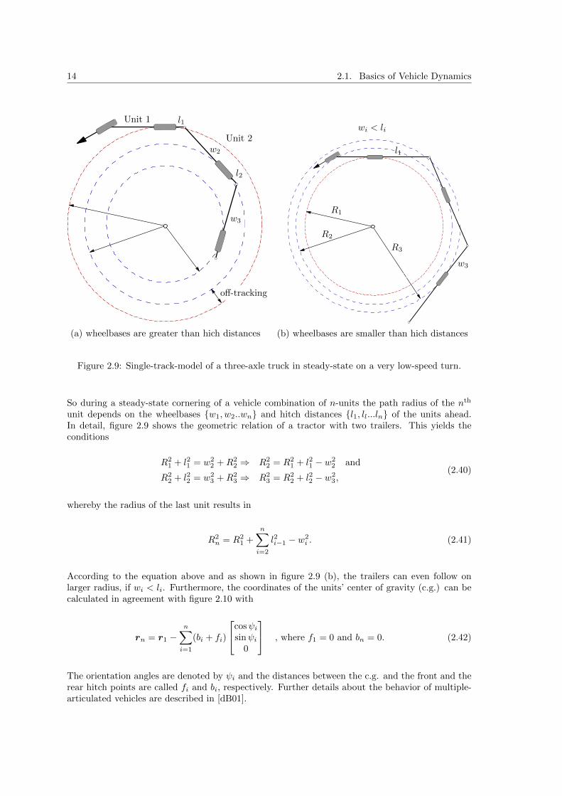
Figure 2.9: Single-track-model of a three-axle truck in steady-state on a very low-speed turn.
So during a steady-state cornering of a vehicle combination of n-units the path radius of the nth
unit depends on the wheelbases w1, w2..wn and hitch distances l1, ll...ln of the units ahead.In detail, figure 2.9 shows the geometric relation of a tractor with two trailers. This yields theconditions
R21 + l21 = w2
2 +R22 ⇒ R2
2 = R21 + l21 − w2
2 and
R22 + l22 = w2
3 +R23 ⇒ R2
3 = R22 + l22 − w2
3,(2.40)
whereby the radius of the last unit results in
R2n = R2
1 +
n∑i=2
l2i−1 − w2i . (2.41)
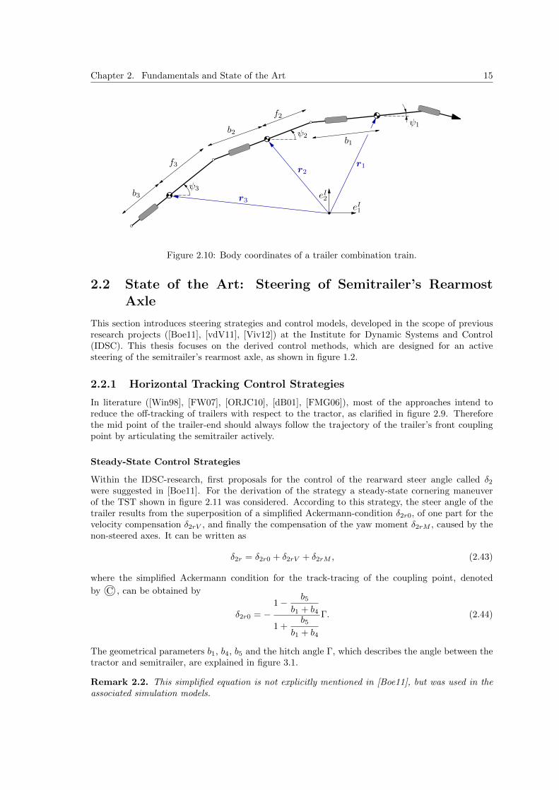
According to the equation above and as shown in figure 2.9 (b), the trailers can even follow onlarger radius, if wi < li. Furthermore, the coordinates of the units’ center of gravity (c.g.) can becalculated in agreement with figure 2.10 with
rn = r1 −n∑i=1
(bi + fi)
cosψisinψi
0
, where f1 = 0 and bn = 0. (2.42)
The orientation angles are denoted by ψi and the distances between the c.g. and the front and therear hitch points are called fi and bi, respectively. Further details about the behavior of multiple-articulated vehicles are described in [dB01].
Chapter 2. Fundamentals and State of the Art 15
f2
b2
b3
f3
b1
ψ1
ψ2
ψ3
eI1
eI2r3
r2r1
Figure 2.10: Body coordinates of a trailer combination train.
2.2 State of the Art: Steering of Semitrailer’s RearmostAxle
This section introduces steering strategies and control models, developed in the scope of previousresearch projects ([Boe11], [vdV11], [Viv12]) at the Institute for Dynamic Systems and Control(IDSC). This thesis focuses on the derived control methods, which are designed for an activesteering of the semitrailer’s rearmost axle, as shown in figure 1.2.
2.2.1 Horizontal Tracking Control Strategies
In literature ([Win98], [FW07], [ORJC10], [dB01], [FMG06]), most of the approaches intend toreduce the off-tracking of trailers with respect to the tractor, as clarified in figure 2.9. Thereforethe mid point of the trailer-end should always follow the trajectory of the trailer’s front couplingpoint by articulating the semitrailer actively.
Steady-State Control Strategies
Within the IDSC-research, first proposals for the control of the rearward steer angle called δ2were suggested in [Boe11]. For the derivation of the strategy a steady-state cornering maneuverof the TST shown in figure 2.11 was considered. According to this strategy, the steer angle of thetrailer results from the superposition of a simplified Ackermann-condition δ2r0, of one part for thevelocity compensation δ2rV , and finally the compensation of the yaw moment δ2rM , caused by thenon-steered axes. It can be written as
δ2r = δ2r0 + δ2rV + δ2rM , (2.43)
where the simplified Ackermann condition for the track-tracing of the coupling point, denoted
by jC , can be obtained by
δ2r0 = −1− b5
b1 + b4
1 +b5
b1 + b4
Γ. (2.44)
The geometrical parameters b1, b4, b5 and the hitch angle Γ, which describes the angle between thetractor and semitrailer, are explained in figure 3.1.
Remark 2.2. This simplified equation is not explicitly mentioned in [Boe11], but was used in theassociated simulation models.

16 2.2. State of the Art: Steering of Semitrailer’s Rearmost Axle
Mfm
αm2
Cαr2
ay
Cαm2
Cαf2Cαf1
Cαr1
αf2
αr2
top view
jC
jE
Figure 2.11: Steady-state control strategy according to [vdV11].
The part of the velocity compensation in (2.43) results in
δ2rV = (m1 +m2)b1(Cαf1 + Cαr1)− b4Cαr2
(b1 + b4)(Cαf1 + Cαr2)Cαr2ay, (2.45)
whereby the centrifugal acceleration is characterized by ay. The mass of the tractor and trailerare denoted with m1 and m2. The quantities Cαf1, Cαr1, Cαf2, Cαm2 and Cαr2 characterize thecornering stiffness at the tractor’s front, rear and the trailer’s front, mid and rear axle. In [Boe11]it is also proposed, that the compensation of the yaw moment can be determined with
δ2rM =αm2Cαm2(b1 + b3) + αf2Cαf2(b1 + b2)
Cαr2(b1 + b4), (2.46)
whereby the slip angles can be approximated with
αf2 = −2(b1 + b2)− (b5 + b1 + b3 + l3 − l2)
b5 + b1 + b3 − (l3 − l2)Γ and (2.47)
αm2 = −2(b1 + b3)− (b5 + b1 + b3 + l3 − l2)
b5 + b1 + b3 − (l3 − l2)Γ. (2.48)
In the following this steady-state control strategies will be named as “feed-forward-controller”,since they don’t compensate any measured error or feedback but just react proportional to thehitch angle Γ.
Path-Following Control Strategies
Moreover, a linear quadratic regulator (LQR)-controller is designed in [vdV11] in order to minimizethe transient off-tracking for the three-axle trailer with a feedback control system.Similarly, in [CC08] a virtual driver steering controller is proposed to control the steering angles oftrailer wheels, so as to make the trailer rear end follow the trajectory of 5th-wheel. The “virtual

Chapter 2. Fundamentals and State of the Art 17
trailer-driver” is assumed to “sit” at the rear end of the semi-trailer and to use preview informationconsisting of path-tracking deviations of the trailer body relative to the trajectory of 5th-wheel. The“virtual driver” model for the trailer steering control is introduced to minimise the path-trackingdeviation of the trailer’s rear end by using a LQR-method. This linear quadratic regulator-approachoptimize a cost function which contains weighted input and output states. For the same purposea PID-Controller with a “reference trailer” is used in [ORJC10]. Thereby the controlled system isinvestigated for low and high velocity.
At last, in the context of the IDSC-research project an additional thesis [Viv12] exists. It analyzeshow the usage of a steerable trailer axle can be beneficial during reversing maneuvers. In conclusion,different feed-forward controllers, feedback controllers, observers and switching strategies particularfor the reverse driving problem are developed and tested. In the following this path-following controlstrategies will be named as “feed-back-controller”, since they compensate a measured deviation,which is returned by a feedback.
2.2.2 Rollover Prevention Control
Since a few years, researchers of different institutions are developing a variety of steering strategiesfor the rollover avoidance of single-unit trucks or tractor-semitrailers. Usually the main challengeis to influence and improve the roll dynamics of these vehicles using the tractor-front or / and asemitrailer rear axle steering.
Roll-Controller for Single-Unit Trucks
In [AO98], [AO99] and [OBA99] control laws for an rollover avoidance of trucks are introduced.Thereby a small auxiliary steering angle is set by an actuator, in addition to the driver’s steeringangle. The control law is based on proportional feedback of the roll rate and the roll acceleration,so that the vehicle’s roll damping is robustly improved for a wide range of speed and height of thecenter of gravity. Furthermore a rollover coefficient (or so-called load transfer ratio LTR) is definedthat basically depends on the lateral acceleration at the center of gravity of the vehicle’s sprungmass. For critical values of this variable an emergency steering and braking system is activated.
Roll-Controller for Tractor-Semitrailer
In [KS88] it was found that the stability of tractor-semitrailer systems at high speeds can besignificantly improved by the usage of a LQR-controller acting on the tractor-front and trailer-rearaxle. Furthermore, some extended LQR-control strategies are designed and investigated, whichreduce the rollover occurrence [Sam00].
In order to minimise a combination of the path-tracking deviation of the trailer rear end relative tothe path of the hitch point (5th-wheel) and the lateral acceleration of trailer c.g. a LQR-controlleris introduced in [CC08]. Thereby the lateral acceleration of trailer c.g. is included as an additionalobjective of the optimal controller in order to improve roll stability. In [ORJC10] this strategiesare extended and investigated for low and high velocities. Finally a similar approach which uses anoptimal controller is introduced and tested in [vdV11].
2.3 Basics of Applied Mechanics and System Dynamics
This section gives an overview of the basic model representations which are important in the scopeof this work. The theory and formulations are extracted from [PS10] and [Lun08].
Usually, the dynamics of a mechanical system can be described by ordinary differential equations.They can be derived applying the principle laws of the physics and mechanics. In considerationof a holonomic rigid MultiBody System (MBS), the motion behavior is completely described by
18 2.3. Basics of Applied Mechanics and System Dynamics
f -generalized coordinates q, whereby f is the number number of degrees of freedom [PS10]. Thenonlinear equations of motion of an ordinary MBS can be read as
M(q, t) q + k(q, q, t) = qe(q, q,u, t), (2.49)
where M is the f × f symmetric inertia matrix, k is a f × 1-vector of generalized gyroscopic forcesincluding the Coriolis and centrifugal forces as well as the gyroscopic torques, and the f×1-vector qe
represents generalized applied forces. Furthermore, equation (2.49) can be rearranged to
⇒ q = M−1(qe − k) (2.50)
and consequently transformed into the nonlinear state-space representation
[q
q
]︸︷︷︸xNonLin
=
[q
M−1(qe − k)
]︸ ︷︷ ︸f (xNonLin,u,t)
, (2.51)
where xNonLin is called the state vector and u denominates the input vector of the nonlinear system.In contrast, equation (2.49) can be linearized to
M(t) qlin + P (t) qlin + Q(t) qlin = H(t)u, (2.52)
where M is the symmetric, positive definite inertia matrix. The matrices P and Q characterize thevelocity and position dependent forces and the matrix H applied by the input vector u representsthe external excitation. The super-scripted “∼” marks the linearity of the matrices. Moreover, thislinear representation can also be rearranged and transformed to a linear state-space representationqlin
qlin
︸ ︷︷ ︸x
=
0 I
−M−1Q −M−1
P
︸ ︷︷ ︸
A
qlin
qlin
︸ ︷︷ ︸x
+
0
M−1H
︸ ︷︷ ︸
B
u, (2.53)
where x is the state vector of the linear model. According to [Lun08] the linear state-space repre-sentation of a system with multiple inputs and multiple outputs (MiMo) generally results in
x = Ax+Bu
y = Cx+Du,(2.54)
where A is called the “system matrix”, B is named as “input matrix”, C is denoted as “outputmatrix” and D is the“feedthrough matrix” according to the system theories.In the case of a system with a single input and a single output (SISO) the linear state-spacerepresentation can be simplified to
x = Ax+ bu
y = cx+ du,(2.55)
where b is a column vector and c is a row vector. The scalar feedthrough is named d. In orderto consider the system in the frequency domain, the transfer function can be calculated from theSISO-state-space model (2.55) by
G(s) = cT (sI −A)−1b+ d. (2.56)

Chapter 3
Modelling
In order to simulate the behaviour of a tractor-semitrailer vehicle (TST) and develop control strate-gies for various driving manoeuvres, mathematical models based on physical laws are required. Thedynamic motion of these models are characterized by the so-called equations of motions. This chap-ter derives a nonlinear and linear horizontal planar model to describe the lateral and yaw motionof the vehicle at low-speed. In addition, the derived models will be extended in order to take alsothe roll motions of the system at high-speed into account. Thereby the TST is always consideredas a rigid Multibody System (MBS).
3.1 Nonlinear Single-Track Model
This section deals with the derivation of a nonlinear horizontal planar model according to the theoryof MBS [PS10]. In previous student theses [Boe11]&[Viv12] within the same research project atthe IDSC, the regarding nonlinear equations were derived on the one hand with the Newton-Euler approach and on the other hand with the Lagrangian approach. This thesis presents thedetailed derivation of the nonlinear equations of motions according to the Newton-Euler approachin subsection 3.1.1. In addition to this, the Lagrangian approach is represented in the subsection A.3with the same result.
The assumptions and simplifications for the nonlinear model are:
• The tires on each axle are combined into one single tire, which is considered to be at thecenter of the axle (single-track model).
• Only the lateral forces of the tires are taken into account: Ftire = Fy (There are no brakingor accelerating forces on the wheels.)
• The lateral tire behavior is considered fully-linear (or linear-saturated) to the related slipangles: Fy ∝ α (and Fy ≤ Fy,max).
• An auxiliary force Faux is used in order to drive the vehicle at constant velocity. It is assumedthat this force is known, since it will later be realized with a subordinate control loop and itis necessary for a later comparison of the different models.
• Pitch and bounce motions have small effects on the vehicle and therefore they are neglected.
• Crosswind and road camber effects are neglected.
• The coupling point (5th-wheel) is considered as a rigid connection and both vehicles as rigidbodies.
19

20 3.1. Nonlinear Single-Track Model
ψ1
ψ2
l1
l3
b1 l2b2
b3
b4
m2
m1
I1
I2
r2
r1
δ1
δ2
Fyf1
Fyr1
Fyr2
Fym2
Fyf2
Faux
x
y
OI
b5
E
CΓ
Figure 3.1: Top view of the Single Track Model of a Tractor and Semitrailer(TST) with a steeredrearmost axle.
In the first step the planar motion of the TST in the inertial frame OI will be described. As shown
in figure 3.1, the distance from the tractor’s front wheel, 5th-wheel jC and rear wheel to the centerof gravity is denoted as l1, l2 and l3. The distance of the 5th-wheel, front wheel, middle wheel andrear wheel of the trailer to it’s center of gravity is named as b1, b2, b3 and b4. The spacing between
the rear wheel and the end of the trailer jE is denoted by b5. The position of the centers of gravityof the tractor and semitrailer are
r1 =
[x2 + b1 cosψ2 + l2 cosψ1
y2 + b1 sinψ2 + l2 sinψ1
]and r2 =
[x2
y2
], (3.1)
where the coordinate tuples x2 and y2 define the position of the tractor. The yaw angle of thesemitrailer and tractor is called ψ2 and ψ1. The tractor has the mass m1, moment of inertia I1 andsteer angle δ1 at the front wheel. In analogy, the semitrailer has the mass m2, moment of inertia I2and steer angle δ2 at the rearward wheel. The tire cornering forces Fyf1 and Fyr1 act at the frontand rear wheel of the tractor, whereby the forces Fyf2, Fym2 and Fyr1 appear at the position ofthe front, middle and rear axle of the semitrailer.
3.1.1 Equations of motion according to the Newton-Euler Approach
In this section the nonlinear model is derived systematically with the Newton-Euler approach asstated in [SW99]. The proposed method is structured in a certain way and the MBS will now beconsidered as a three-dimensional system in order to explain the structure generally. Therefore theposition vectors to the centers of gravity will be redefined to
r1 =
x2 + b1 cosψ2 + l2 cosψ1
y2 + b1 sinψ2 + l2 sinψ1
0
and r2 =
x2
y2
0
. (3.2)

Chapter 3. Modelling 21
With the generalized coordinates q =[x2 y2 ψ2 ψ1
]T, the translational Jacobian matrices JT1
and JT2 for the tractor and semitrailer can be evaluated with
JT1 =∂r1
∂q=
1 0 −b1 sinψ2 −l2 sinψ1
0 1 b1 cosψ2 l2 cosψ1
0 0 0 0
and JT2 =∂r2
∂q=
1 0 0 00 1 0 00 0 0 0
. (3.3)
This leads to the conclusion that the velocity and acceleration of the kth body are
vk = JTkq +∂rk
∂t︸︷︷︸vk
and ak = JTkq + JTkq +∂vk
∂t︸ ︷︷ ︸ak
, (3.4)
whereby vk and ak are declared as the local velocity and local acceleration. Due to the fact that anybody rotation is not explicit time dependent, the vector of the corresponding angular velocity ωkcan be described by the rotational Jacobian matrix JRk and the time derivative of the generalizedcoordinates,
ω1 =
00
ψ1
=
0 0 0 00 0 0 00 0 0 1
︸ ︷︷ ︸
JR1
q and ω2 =
00
ψ2
=
0 0 0 00 0 0 00 0 1 0
︸ ︷︷ ︸
JR2
q. (3.5)
As reported by [SW99], the equations of motions can be expressed in block matrices,m1E sym.
0 m1E0 0 I1
0 0 0 I2
︸ ︷︷ ︸
M
JT1
JT2
JR1
JR2
︸ ︷︷ ︸J
q +
m1a1
m2a2
I1α1 + ω1I1ω1
I2α2 + ω2I2ω2
︸ ︷︷ ︸
k
=
fe1fe2le1le2
︸ ︷︷ ︸qe
+
fr1fr2lr1lr2
︸ ︷︷ ︸qr
. (3.6)
Each line characterize the force balance in the direction of a Cartesian coordinate of one body. Thesymmetrical matrix M contains the mass and the inertia tensors
I1 =
Ixx1 Ixy1 Ixz1Ixy1 Iyy1 Iyz1Ixz1 Iyz1 I1
and I2 =
Ixx2 Ixy2 Ixz2Ixy2 Iyy2 Iyz2Ixz2 Iyz2 I2
. (3.7)
Besides the specified Jacobian matrices are composed to the global Jacobian matrix J . Further-more k denotes the vector of Coriolis and gyroscopic forces and torques, where ak and αk denomi-nate the local acceleration and local angular acceleration. The rotation of the bodies is not explicitlytime dependent and they spin around their mass centroid axis, so the terms Ikαk + ωkIkωk dis-appear. The vector qe presents the applied forces and moments which results from the tires. Inaddition qr contains the reaction forces and moments. The 12 equations stated in (3.6) can bereduced to the minimal number of four ordinary differential equations by a left pre-multiplicationwith the transposed global Jacobian matrix JT ,
JTMJ︸ ︷︷ ︸M
q + JT k︸︷︷︸k
= JT qe︸ ︷︷ ︸qe
+
JT Qg︸ ︷︷ ︸qr
. (3.8)
With that step the reaction forces disappear because of the generalized orthogonality betweenmotion and constraint, i.e. vanishing virtual work of the reaction forces (JT Q = 0) [PS10]. Forthe current MBS the only challenge is to evaluate the local accelerations
a1 =
−l2cψ1ψ21 − b1cψ2 ψ
22
−l2sψ1ψ21 − b1sψ2
ψ22
0
and a2 =
000
(3.9)

22 3.1. Nonlinear Single-Track Model
and take the applied forces of the tires acting on the centers of gravity into account. They can beexpressed in Cartesian coordinates with
qe =
Fyf1sψ1+δ1 + Fyr1sψ1+ Fauxcψ1
−Fyf1cψ1+δ1 − Fyr1cψ1 + Fauxsψ1
0Fyf2sψ2
+ Fym2sψ2+ Fyr2sψ2+δ2
−Fyf2cψ2− Fym2cψ2
− Fyr2cψ2+δ2
000
−Fyf1l1cδ1 + Fyr1l300
Fyf2b2 + Fym2b3 + Fyr2b4cδ2
. (3.10)
The trigonometric functions are notated according to (A.1). In conclusion, after some calculationthe equations of motion in matrix-form and conform to (2.49) results inm1 +m2 0 −m1b1sψ2
−m1l2sψ1
0 m1 +m2 m1b1cψ2 m1l2cψ1
−m1b1sψ2 m1b1cψ2 m1b21 + I2 m1l2b1cψ1−ψ2
−m1l2sψ1m1l2cψ1
m1l2b1cψ1−ψ2m1l
22 + I1
q +
−m1l2cψ1
ψ21 −m1b1cψ2
ψ22
−m1l2sψ1 ψ21 −m1b1sψ2 ψ
22
−m1ψ21l2b1sψ1−ψ2
m1ψ22l2b1sψ1−ψ2
...
=
Fyf1sδ1+ψ1 + Fyr2sδ2+ψ2 + Fyf2sψ2 + Fym2sψ2 + Fyr1sψ1 + Fauxcψ1
−Fyf1cδ1+ψ1 − Fyr2cδ2+ψ2 − Fyf2cψ2 − Fym2cψ2 − Fyr1cψ1 + Fauxsψ1
Fyf2b2 + Fym2b3 − Fyr1b1cψ1−ψ2− Fyf1b1cδ1+ψ1−ψ2
+ Fyr2b4cδ2 + Fauxb1sψ1−ψ2
Fyr1(l3 − l2)− Fyf1cδ1(l1 + l2)
.
(3.11)
In comparison with (A.24), these derived equations of motions are identical.
3.1.2 Transformation to trailer-fixed reference frame
Up to this point, a full non-linear model for the planar motion in the inertial frame is derived.Nevertheless, for the purpose of creating a controller, it is necessary to have all the equationsexpressed in a frame fixed to one of the two truck units. Since this work mainly focus on thesemitrailer, a trailer-fixed reference frame is used. The new vector of generalized coordinates is
Sq =
[Sx2 S
y2 ψ2 ψ1
]T, (3.12)
whereSx2 and
Sy2 denotes the trailer position with respect to the semitrailer coordinate system OS ,
which is fixed to its center of gravity. Figure 3.2 shows the model description at two points oftime (t(k) and t(k+1)) during a simulation process. Consequently the position of the semitrailerwith respect to the initial frame OI at t(k+1) can be expressed by
r(k+1)2 =
[x2
y2
]= r
(k)2 +
[cosψ
(k)2 − sinψ
(k)2
sinψ(k)2 cosψ
(k)2
]︸ ︷︷ ︸
IφSψ(k)2
[S∆x2
S∆y2
]︸ ︷︷ ︸S
∆r2
, (3.13)
where r(k)2 is the previous position at t(k) and IφS the rotational matrix of the semitrailer. More-
overS∆r2 is the relative displacement after the time-step ∆t. With the velocity
Sr2 =
[Sx2 S
y2
]Tit yields
S∆r2 =
Sr2 ∆t. (3.14)

Chapter 3. Modelling 23
ψ(k)1
ψ(k)2
r(k)2
r(k)1
xy
Sx
Sy
Ty
TxOI
OS
OT
r(k+1)2
r(k+1)1
ψ(k+1)1
ψ(k+1)2
Timepoint: t = t(k)
Timepoint: t(k+1) = t(k) + ∆t
S∆x2 , S x2
S∆y2 , S y2
Coordinate tuples & velocities
with respect to OS
Γ = hitch angle
S∆r2,
Sr2
Figure 3.2: Coordinate transformation of the TST-Single Track Model.
Since theS∆r2 and
Sr2 have the same direction, the velocity with respect to OI and OS are also
related to the rotational matrix of the semitrailer IφS ,
[x2
y2
]︸︷︷ ︸v2
=
[cosψ2 − sinψ2
sinψ2 cosψ2
]︸ ︷︷ ︸
IφS(ψ2)
[Sx2
Sy2
]︸ ︷︷ ︸Sv2
. (3.15)
When considering the angle velocities it is obvious, that they are independent of the referenceframe (ψ1 =
Sψ1 and ψ2 =
Sψ2). This leads to the transformation matrix IΦS , which describes
the relation between the previous and current generalized velocities,
x2
y2
ψ2
ψ1
︸ ︷︷ ︸q
=
cosψ2 − sinψ2 0 0sinψ2 cosψ2 0 0
0 0 1 00 0 0 1
︸ ︷︷ ︸
IΦS
Sx2
Sy2
ψ2
ψ1
︸ ︷︷ ︸Sq
. (3.16)
Furthermore it yields SΦI = IΦS−1 = IΦS
T , since the linear transformation IΦS is orthogonal.Applying (3.16) to (3.8) it is possible to obtain the equations of motion expressed in the trailer-fixedreference frame in matrix form,
SΦIM IΦS︸ ︷︷ ︸SM
Sq + SΦIM IΦS S
q + SΦI k︸ ︷︷ ︸Sk
= SΦI qe︸ ︷︷ ︸
Sqe
. (3.17)

24 3.2. Model Extensions and Background Analysis
After some calculations the equations of motions with reference to the trailer-fixed frame results inm1 +m2 0 0 −m1l2sΓ
0 m1 +m2 m1b1 m1l2cΓ
0 m1b1 m1b21 + I2 m1l2b1cΓ
−m1l2sΓ m1l2cΓ m1l2b1cΓ m1l22 + I1
S q +
−m1ψ
22b1 −m1ψ
21l2cΓ−(m1+m2)ψ2 S y2
−m1ψ21l2sΓ + ψ2 (m1 +m2)S x2
m1b1(ψ2 S x2 − ψ21l2sΓ)
m1ψ2l2(S x2 cΓ + (S y2 + ψ2b1)sΓ)
...
=
Fyf1sδ1+Γ + Fyr2sδ2 + FauxcΓ + Fyr1sΓ
FauxsΓ − Fyf2 − Fym2 − Fyf1cδ1+Γ − Fyr2cδ2 − Fyr1cΓ
Fyf2b2 + Fym2b3 − Fyr1b1cΓ + Fauxb1sΓ − Fyf1b1cδ1+Γ + Fyr2b4cδ2Fyr1(l3 − l2) − Fyf1cδ1(l1 + l2)
, where
(3.18)
Γ = ψ1 − ψ2 (3.19)
denotes the hitch angle and the trigonometric functions are notated in agreement with (A.1).
3.2 Model Extensions and Background Analysis
3.2.1 Trajectories with respect to the Initial Reference Frame
The model equations according to (3.18) are formulated with respect to the semitrailer-fixed refer-ence frame OS . In order to identify the positions of the semitrailer and tractor units, the trajectoriesin the inertial reference frame OI must be obtained by the generalized coordinates of the simulationresults. Additionally, the following back transformation method is also needed for the determinationof the tire forces, at each simulation time-step.Given are the generalized positions in line with (3.12)and along a simulated time line t(1)...t(k)...t(n),
Sqresult =
Sx
(1)2 S
x(2)2 ...
Sx
(k)2 S
x(k+1)2 ...
Sx
(n)2
Sy
(1)2 S
y(2)2 ...
Sy
(k)2 S
y(k+1)2 ...
Sy
(n)2
ψ(1)2 ψ
(2)2 ... ψ
(k)2 ψ
(k+1)2 ... ψ
(n)2
ψ(1)1 ψ
(2)1 ... ψ
(k)1 ψ
(k+1)1 ... ψ
(n)1
. (3.20)
The kth displacement vector of the semitrailer unit relative to OS can be evaluated by
S∆r
(k)2 =
[Sx
(k+1)2 −
Sx
(k)2
Sy
(k+1)2 −
Sy
(k)2
], for k = 1(1)n− 1. (3.21)
In consideration of the initial condition r02 and (3.13), the trailer position with respect to the initialreference frame can be calculated,
r(k)2 =
r02 for k = 1
r(k−1)2 + IφS(ψ
(k−1)2 )
S∆r
(k−1)2 for k = 2(1)n,
(3.22)
where IφS(ψ(k−1)2 ) denotes the rotation matrix of the semitrailer with the applied angle ψ
(k−1)2 .
Figure 3.2 clarifies the relations again. The trailer position can be alternatively obtained by trans-forming the relative trailer velocity
Sv2 to the velocity in the initial reference frame v2 using
equation (3.15) and applying an integration in the form of
r2 =
∫v2 dt, (3.23)
or for discrete values:
r(k)2 =
r02 for k = 1
r(k−1)2 + v
(k−1)2 ∆t(k−1) for k = 2(1)n.
(3.24)

Chapter 3. Modelling 25
This thesis also treats a linear model with the generalized coordinates
qlin =[Γ ψ1 β2 ψ2
]T. (3.25)
Since this model assumes a constant body velocity v, the semitrailer velocity in the initial referenceframe results in
v2 =
[x2
y2
]=
[v cos(β2 + ψ2)v sin(β2 + ψ2)
]. (3.26)
The semitrailer position can be calculated afterwards, using equation (3.23), for discrete val-ues (3.24) respectively.In conclusion, the trajectory of the tractor’s c.g. can be obtained by (3.1), in detail it results
r(k)1 = r
(k)2 +
[b1 cosψ
(k)2 + l2 cosψ
(k)1
b1 sinψ(k)2 + l2 sinψ
(k)1
], for k = 1(1)n. (3.27)
3.2.2 Tire Forces and Kinematic Constraints
In order to determine the tire forces during the simulation process, some kinematic relations haveto be taken into account. As already discussed in section 2.1.1, the tire forces Fαi of the modeledTST linearly depend on the corresponding slip angles αi,
Fyf1 = Cαf1 αf1 Fyr1 = Cαr1 αr1 (3.28)
Fyf2 = Cαf2 αf2 Fym2 = Cαm2 αm2 Fyr2 = Cαr2 αr2 (3.29)
for the tractor and for the semitrailer, where Cαi is the cornering stiffness for the single axles.
Remark 3.1. The tire forces can be either regarded fully linear as stated in (2.5) or saturatedaccording to (2.6). This distinction is especially important for the derivative of the linear modelreported by section 3.3. Conveniently, it will treated as fully linear during this section.
In analogy to (2.16), the resulting slip angles are
αf1 = δ1 −ψ1l1|Tv1|− β1 αr1 =
ψ1l3|Tv1|− β1 (3.30)
αf2 =ψ2b2|Sv2|− β2 αm2 =
ψ2b3|Sv2|− β2 αr2 = δ2 +
ψ2b4|Sv2|− β2, (3.31)
where the constant distances are depicted in figure 3.1,Tv1 = [
Tx1 T
y1]T andSv2 = [
Sx2 S
y2]T
are the body velocities and β1 (]Tx1, T y1) and β2 (]
Sx2, S y2) are the body slip angles. Since
Sx2
andSy2 are generalized coordinates, the vector norm and body slip angle of the semitrailer are also
known as
|Sv2| =
√Sx2
2 +Sy2
2 (= v2) and β2 = arctan
(Sy2
Sx2
). (3.32)
Before the calculation of the tractor’s body slip angle it is necessary to obtain the tractor velocity v1
represented in the initial reference frame. This can be done with the derivative of (3.27) with respectto the time,
r1︸︷︷︸v1
= r2︸︷︷︸v2
+
[−ψ2b1 sinψ2 − ψ1l2 sinψ1
ψ2b1 cosψ2 + ψl2 cosψ1
]︸ ︷︷ ︸
vψ
, (3.33)
26 3.2. Model Extensions and Background Analysis
r1
xy
OI
OS
OT
r2
ψ2
v2
v1
ψ1
v2
v1vψ
β1
β2
(a) Detail of TST hitch kinematic (b) Top view of Single-Track TST
b1
l2
OT
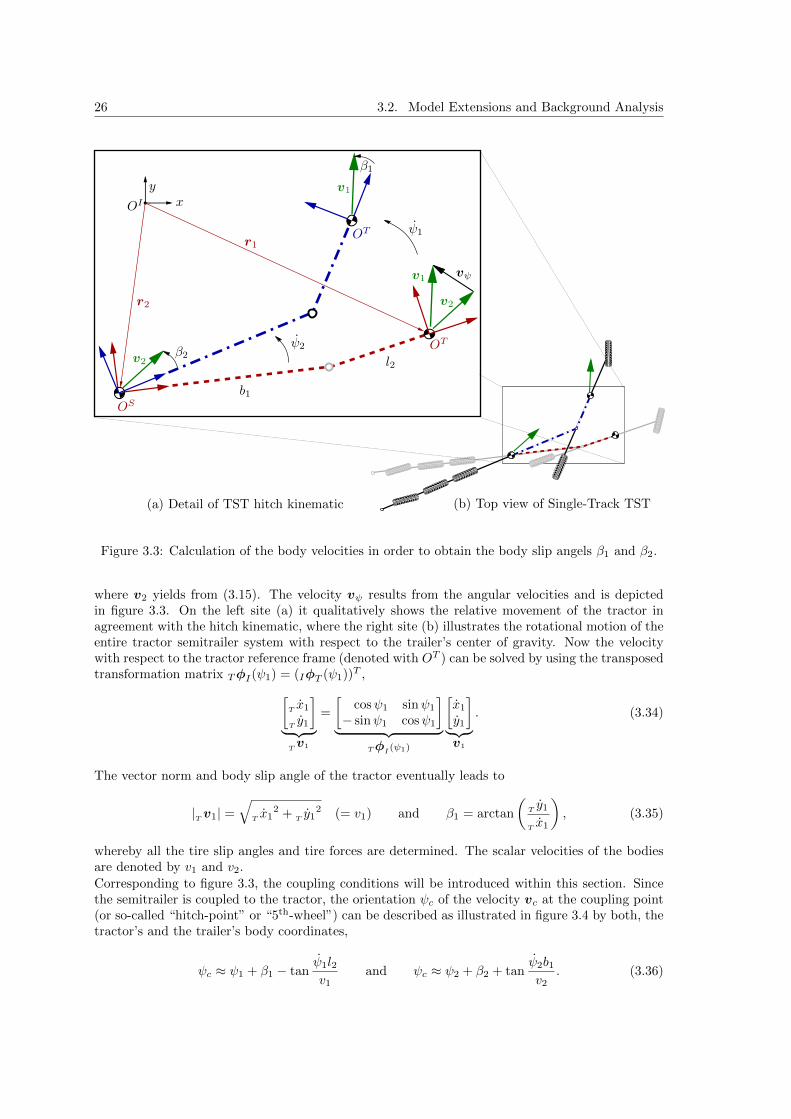
Figure 3.3: Calculation of the body velocities in order to obtain the body slip angels β1 and β2.
where v2 yields from (3.15). The velocity vψ results from the angular velocities and is depictedin figure 3.3. On the left site (a) it qualitatively shows the relative movement of the tractor inagreement with the hitch kinematic, where the right site (b) illustrates the rotational motion of theentire tractor semitrailer system with respect to the trailer’s center of gravity. Now the velocitywith respect to the tractor reference frame (denoted with OT ) can be solved by using the transposedtransformation matrix TφI(ψ1) = (IφT (ψ1))T ,[
Tx1
Ty1
]︸ ︷︷ ︸Tv1
=
[cosψ1 sinψ1
− sinψ1 cosψ1
]︸ ︷︷ ︸
TφI(ψ1)
[x1
y1
]︸︷︷ ︸v1
. (3.34)
The vector norm and body slip angle of the tractor eventually leads to
|Tv1| =
√Tx1
2 +Ty1
2 (= v1) and β1 = arctan
(Ty1
Tx1
), (3.35)
whereby all the tire slip angles and tire forces are determined. The scalar velocities of the bodiesare denoted by v1 and v2.Corresponding to figure 3.3, the coupling conditions will be introduced within this section. Sincethe semitrailer is coupled to the tractor, the orientation ψc of the velocity vc at the coupling point(or so-called “hitch-point” or “5th-wheel”) can be described as illustrated in figure 3.4 by both, thetractor’s and the trailer’s body coordinates,
ψc ≈ ψ1 + β1 − tanψ1l2v1
and ψc ≈ ψ2 + β2 + tanψ2b1v2
. (3.36)

Chapter 3. Modelling 27
OT
v1−ψ1
β1
l2
OS
ψ2
v2 β2b1ψ2
ψ1
v2
vc vc−ψ1l2
ψ2 b1
ψc ψc
(b) Tractor and 5th-wheel velocities(a) Semitrailer and 5th-wheel velocities
v1
Figure 3.4: Top view of the hitch kinematic for the derivation of the coupling condition.
With the simplification tan] ≈ ] and the elimination of the angle ψc, the kinematic constraintequation results equal to [SC98] with
ψ1 + β1 −ψ1l2v1≈ ψ2 + β2 +
ψ2b1v2
⇔ β1 ≈ −Γ + β2 +ψ2b1v2
+ψ1l2v1
, (3.37)
where Γ is defined in (3.19). The derivation with respect to the time and assuming v1 = 0 and v2 =0, yields
ψ1 + β1 −ψ1l2v1≈ ψ2 + β2 +
ψ2b1v2
⇔ β1 ≈ ψ2 − ψ1 + β2 +ψ2b1v2
+ψ1l2v1
. (3.38)
If the roll motion of the tractor semitrailer should also be taken into account, the model can beextend to a so-called “yaw-roll”-model. The 3D-position of the 5th-wheel can be described witheither
rc1 =
x1 − l2 cosψ1 + z1 sinφ1 sinψ1
y1 − l2 sinψ1 − z1 sinφ1 cosψ1
z1 cosφ1
or rc2 =
x2 + b1 cosψ2 + z2 sinφ2 sinψ2
y2 + b1 sinψ2 − z2 sinφ2 cosψ2
z2 cosφ2
, (3.39)
whereby φ1 and φ2 are the roll angle of the tractor and semitrailer. The distances from the rollaxis to the 5th-wheel is denoted by z1 and z2, respectively. Furthermore, it is assumed that theposition of the tractor’s c.g. is given with x1 and y1. The derivative with respect to the time leadsto the velocities
vc1 =
x1 + ψ1l2 sinψ1 + φ1z1 cosφ1 sinψ1 + ψ1z1 sinφ1 cosψ1
y1 − ψ1l2 cosψ1 − φ1z1 cosφ1 cosψ1 + ψ1z1 sinφ1 sinψ1
−φ1z1 sinφ1
and (3.40)
vc2 =
x2 − ψ2b1 sinψ2 + φ2z2 cosφ2 sinψ2 + ψ2z2 sinφ2 cosψ2
y2 + ψ2b1 cosψ2 − φ2z2 cosφ2 cosψ2 + ψ2z2 sinφ2 sinψ2
−φ2z2 sinφ2
. (3.41)
The velocity components of the c.g.’s of the tractor and semitrailer can also be written as
x1 = v1 cos(ψ1 + β1) y1 = v1 sin(ψ1 + β1) , and (3.42)
x2 = v2 cos(ψ2 + β2) y2 = v2 sin(ψ2 + β2). (3.43)

28 3.2. Model Extensions and Background Analysis
OTv1
−ψ1
β1
l2
OS
ψ2
v2 β2
b1ψ2
ψ1
v2vc
−ψ1l2ψ2 b1
ψcψc
(b) Tractor and 5th wheel velocities(a) Semitrailer and 5th wheel velocities
v1 vc
φ2 z2
φ2
OI
φ1φ1 z1
ψ2 b1 − φ2 z2 −ψ1l2 − φ1 z1
xyz
x2
y2
x1
y1
z2
z15th5th
Figure 3.5: 3D view of the hitch kinematic for the derivation of the coupling condition for a yaw-rollmodel.
Moreover, the velocities can be represented in the body-fixed reference frames (rotation with ψ1
or ψ2 around the z-axis), which leads to
Tvc1 = TφI vc1 =
v1 cosβ1 + ψ1z1 sinφ1
v1 sinβ1 − ψ1l2 − φ1z1 cosφ1
−φ1z1 sinφ1
and (3.44)
Svc2 = SφI vc2 =
v2 cosβ2 + ψ2z2 sinφ2
v2 sinβ2 + ψ2b1 − φ2z2 cosφ2
−φ2z2 sinφ2
. (3.45)
For the consideration of small angles (ψ1, ψ2, φ1, φ2 << 1) the lateral velocities results in
Tvc1y = v1β1 − ψ1l2 − φ1z1 and
Svc2y = v2β2 + ψ2b1 − φ2z2, (3.46)
This relations are clarified in figure 3.5 for the kinematic of the tractor in fig. 3.5(b) and thesemitrailer in fig. 3.5(a). The orientation of the velocities with respect to the body-fixed referenceframes and around the z-axis can be approximated with
Tψc1 = β1 −
ψ1l2v1− φ1z1
v1and
Sψc2 = β2 +
ψ2b1v2− φ2z2
v2. (3.47)
The representation with respect to the initial reference frame can be read as
ψc1 = ψ1 + β1 −ψ1l2v1− φ1z1
v1and ψc2 = ψ2 + β2 +
ψ2b1v2− φ2z2
v2. (3.48)
Since the both hitch description have the same velocity orientation (ψc1!= ψc1), the kinematic
constraint equation (also called algebraic loop) yields
ψ1 − ψ2 + β1 − β2 −l2v1ψ1 −
b1v2ψ2 −
z1
v1φ1 +
z2
v2φ2 = 0. (3.49)

Chapter 3. Modelling 29
In conclusion, the derivation with respect to the time and assuming v1 = 0 and v2 = 0, results in
ψ1 − ψ2 + β1 − β2 −l2v1ψ1 −
b1v2ψ2 −
z1
v1φ1 +
z2
v2φ2 = 0. (3.50)
This constrain equation is also used in e.g. [SC98], [CC08] or [vdV11].
3.3 Linear Single-Track Model
In order to reduce the simulation cost, to develop linear controllers and to use the methods of thelinear system theory, a linear model of the TST will be derived by the nonlinear equations withinthis section. On the one hand subsection 3.3.1 establishes fully linear equations of motion and onthe other hand subsection 3.3.2 introduce a linear model with the saturated tire-force-model. Analternative derivation of the fully linear system is described in section A.5.Assuming the angle between the tractor and semitrailer is very small Γ << 1, it yields
sin(Γ) ≈ Γ and cos(Γ) ≈ 1, (3.51)
it can also be simplified for small steering angles,
sin(δ1) ≈ δ1 and cos(δ1) ≈ 1, (3.52)
sin(δ2) ≈ δ2 and cos(δ2) ≈ 1. (3.53)
The addition theorems can be used in order to linearize the trigonometric functions,
sin(δ1 + Γ) ≈ δ1 + Γ and cos(δ1 + Γ) ≈ 1− Γδ1. (3.54)
With these approximations and neglecting the quadratic terms (ψ22 = 0, ψ2
1 = 0), the nonlinearsystem of equations (3.18) yields
m1 +m2 0 0 00 m1 +m2 m1b1 l2m1
0 m1b1 m1b21 + I2 l2b1m1
0 m1l2 m1l2b1 m1l22 + I1
S x2
S y2
ψ2
ψ1
+
−(m1 +m2)ψ2 S y2
(m1 +m2)ψ2 S x2
m1b1ψ2 S x2
m1ψ2l2(S x2 + (S y2 + ψ2b1) Γ)
...
=
Fyf1(δ1 + Γ) + Fyr2 δ2 + Faux + Fyr1Γ
FauxΓ − Fyf2 − Fym2 − Fyf1(1 − Γδ1) − Fyr2 − Fyr1Fyf2b2 + Fym2b3 − Fyr1b1 + Fauxb1Γ − Fyf1b1(1 − Γδ1) + Fyr2b4
Fyr1(l3 − l2) − Fyf1(l1 + l2)
.
(3.55)
From (A.35), the movement can approximately be expressed with the resulted body velocity v2 andthe body slip angle of semitrailer β2,
Sx2 ≈ v2 and
Sy2 ≈ v2β2, (3.56)
Sx2 ≈ v2 and
Sy2 ≈ v2β2 + v2β2. (3.57)
In the following it will be assumed, that the tractor and semitrailer approximately moves with thesame constant velocity called v, so it yields v1 = v2 = v and v = 0. As a consequence, the auxiliaryforce Faux will become a reaction force and it disappears (for more details go to section 3.1).Furthermore, the product of small angles and angle velocities can be neglected (Γδ1 = β2Γ =ψ2Γ = 0). So the equation (3.55) simplifies to
−(m1 +m2)ψ2 vβ2
(m1 +m2)v(β2 + ψ2) +m1b1ψ2 +m1l2ψ1
b1m1v(β2 + ψ2) + (m1b21 + I2)ψ2 +m1l2b1ψ1
m1l2v(β2 + ψ2) +m1l2b1ψ2 + (m1l22 + I1)ψ1
=
Fyf1(δ1 + Γ) + Fyr2 δ2 + Fyr1Γ−Fyf2 − Fym2 − Fyf1 − Fyr2 − Fyr1
Fyf2b2+Fym2b3+Fyr2b4−(Fyr1+Fyf1)b1Fyr1(l3 − l2)− Fyf1(l1 + l2)
. .(3.58)
In conclusion, the assumptions and simplifications for the linear model can be summarized by:

30 3.3. Linear Single-Track Model
• The tires on each axle are combined into one single tire, which is considered to be at thecenter of the axle (single-track model).
• Only the lateral forces of the tires are taken into account: Ftire = Fy. (There are no brakingor accelerating forces on the wheels.)
• The angle between the tractor and semitrailer is very small: Γ << 1.
• The steer angles of the tractor and semitrailer are very small: δ1 << 1 and δ2 << 1.
• The velocity of each unit is constant: v1 = v2 = v and v = 0.
• The yaw rates are small: ψ1 << 1 and ψ2 << 1.
• Pitch and bounce motions have small effects on the vehicle and are therefore neglected.
• Crosswind and road camber effects are neglected.
• The coupling point (5th-wheel) is considered as a rigid connection without compliance.
3.3.1 Fully Linear Equations of Motions
In the following, a fully linear model will be derived by using the additional assumption:
• The lateral tires behavior is considered fully-linear to the related slip angles: Fy ∝ α.
Since the first equation of (3.58) is of little importance, it can be neglected. The tire forces canbe substituted with (3.28) and (3.29), where the slip angles αi at the tires are explicitly definedin (3.30). Moreover, using the kinematic constraint equation (3.37) for the elimination of β1, theremaining equations of motion results for the second row in
m1l2ψ1 + (m1 +m2)vβ2 +m1b1ψ2 + (Cαf1 + Cαr1)Γ ...
+
(Cαr1
l3 − l2v− Cαf1
l1 + l2v
)ψ1 − (Cαf2 + Cαm2 + Cαr2 + Cαf1 + Cαr1)β2...
+
((m1 +m2)v + Cαf2
b2v
+ Cαm2b3v
+ Cαr2b4v− (Cαf1 + Cαr1)
b1v
)ψ2 = ...
−Cαf1δ1 − Cαr2δ2,
(3.59)
the third row it leads to
m1l2b1ψ1 +m1b1vβ2 + (m1b21 + I2)ψ2 + (Cαr1 + Cαf1)b1Γ ...
+
(Cαr1b1
l3 − l2v− Cαf1b1
l1 + l2v
)ψ1 + (Cαf2b2 + Cαm2b3 + Cαr2b4 − Cαr1b1 − Cαf1b1)β2...
+
(m1vb1 − Cαf2
b22v− Cαm2
b23v− Cαr2
b24v− Cαr1
b21v− Cαf1
b21v
)ψ2 = ...
−Cαf1b1δ1 + Cαr2b4δ2
(3.60)
and the fourth row can be formulated as
(m1l22 + I1)ψ1 +m1l2vβ2 +m1l2b1ψ2 + (Cαf1(l1 + l2)− Cαr1(l3 − l2))Γ ...
+
(−Cαr1
(l3 − l2)2
v− Cαf1
(l1 + l2)2
v
)ψ1 + (Cαr1(l3 − l2)− Cαf1(l1 + l2))β2...
+
(m1l2v + Cαr1b1
l3 − l2v− Cαf1b1
l1 + l2v
)ψ2 = ...
−Cαf1(l1 + l2)δ1.
(3.61)
Chapter 3. Modelling 31
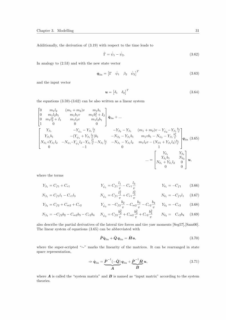
Additionally, the derivation of (3.19) with respect to the time leads to
Γ = ψ1 − ψ2. (3.62)
In analogy to (2.53) and with the new state vector
qlin =[Γ ψ1 β2 ψ2
]T(3.63)
and the input vector
u =[δ1 δ2
]T(3.64)
the equations (3.59)-(3.62) can be also written as a linear system0 m1l2 (m1 +m2)v m1b10 m1l2b1 m1b1v m1b
21 + I2
0 m1l22 + I1 m1l2v m1l2b1
1 0 0 0
qlin + ...
Yβ1
−Yψ1− Yβ1
l2v −Yβ2 − Yβ1 (m1 +m2)v − Yψ2
−Yβ1
b1v
Yβ1b1 −(Yψ1+ Yβ1
l2v )b1 −Nβ2 − Yβ1b1 m1vb1 −Nψ2 − Yβ1
b21v
Nβ1+Yβ1 l2 −Nψ1−Yψ1l2−Yβ1
l22v −Nβ1
l2v −Nβ1 − Yβ1 l2 m1l2v − (Nβ1 + Yβ1 l2) b1v
0 −1 0 1
qlin
... =
Yδ1 Yδ2Yδ1b1 Nδ2
Nδ1 + Yδ1 l2 00 0
u,
(3.65)
where the terms
Yβ1 = Cf1 + Cr1 Yψ1= Cf1
l1v− Cr1
l3v
Yδ1 = −Cf1 (3.66)
Nβ1= Cf1l1 − Cr1l3 Nψ1
= Cf1l21v
+ Cr1l23v
Nδ1 = −Cf1l1 (3.67)
Yβ2= Cf2 + Cm2 + Cr2 Yψ2
= −Cf2b2v− Cm2
b3v− Cr2
b4v
Yδ2 = −Cr2 (3.68)
Nβ2 = −Cf2b2 − Cm2b3 − Cr2b4 Nψ2= Cf2
b22v
+ Cm2b23v
+ Cr2b24v
Nδ2 = Cr2b4 (3.69)
also describe the partial derivatives of the lateral tire forces and tire yaw moments [Seg57],[Sam00].The linear system of equations (3.65) can be abbreviated with
P qlin + Q qlin = Hu, (3.70)
where the super-scripted “∼” marks the linearity of the matrices. It can be rearranged in statespace representation,
⇒ qlin = P−1
(−Q)︸ ︷︷ ︸A
qlin + P−1H︸ ︷︷ ︸
B
u, (3.71)
where A is called the “system matrix” and B is named as “input matrix” according to the systemtheories.

32 3.4. Roll-extended Single-Track Models
3.3.2 Linear Equations of Motion with saturated Tire Forces
In contrast to section 3.3.1, the following assumption yields:
• The lateral tires behavior is considered linear-saturated to the related slip angles: Fy ∝ αand Fy ≤ Fy,max.
This means, that a simplified and linear model is demanded, but the lateral tire forces must berestrictable to certain maximum and minimum values. This can be accomplished regarding thesecond, third and fourth equation of (3.58) and using (3.62). With the state vector
qlin,F =[Γ ψ1 β2 ψ2
]T(3.72)
and the vector of the saturated input forces stated in (2.6) and (3.28)-(3.31),
uF =[Fyf1,sat Fyr1,sat Fyf2,sat Fym2,sat Fyr2,sat
]T, (3.73)
the model equation results in0 m1l2 (m1 +m2)v m1b10 m1l2b1 m1b1v m1b
21 + I2
0 m1l22 + I1 m1l2v m1l2b1
1 0 0 0
︸ ︷︷ ︸
˜P F
qlin,F +
0 0 0 (m1 +m2)v1
0 0 0 m1v1b10 0 0 m1v1l20 −1 0 1
︸ ︷︷ ︸
˜QF
qlin,F ...
=
−1 −1 −1 −1 −1−b1 −b1 b2 b3 b4
−(l1 + l2) (l3 − l2) 0 0 00 0 0 0 0
︸ ︷︷ ︸
˜HF
uF .
(3.74)
This can also be rearranged in state space representation,
⇒ qlin,F = P−1
F (−QF )︸ ︷︷ ︸AF
qlin,F + P−1
F HF︸ ︷︷ ︸BF
uF . (3.75)
Remark 3.2. This model description requires to pre-calculate the tire forces from the current steerangles and generalized coordinates indeed, but also allows to use other tire models.
3.4 Roll-extended Single-Track Models
In order to improve the active safety of semitrailers with a steered rearmost axle, the roll stabilityhas to be investigated. Therefore a nonlinear and linear model will be derived within this section.
3.4.1 Nonlinear Lateral-Yaw-Roll Model
The equations of motion for a precise single-track model of the tractor-semitrailer will be derivedin the following, using the Newton-Euler approach from section 3.1. This model is intended for thevalidation of the linear roll-extended model, which will be introduced later in section 3.4.2.
According to figure 3.6 the position of the centers of gravity of the tractor and semitrailer can be

Chapter 3. Modelling 33
ψ1
ψ2
l1
l3
b1
l2
b2b3
b4
m2
m1I1
I2
r2
r1
δ1
δ2
Fyf1
Fyr1
Fyr2
Fym2
Fyf2
Faux
b5Γ
c1
d1
gm1
h1
lexy2
lexy1(a) Front view of tractor
(c) Top view of tractor and semitrailer
I1
c2
d2
φ2
m2
h2
(b) Front view of semitrailer
I2
cc
OS
x
y
OI
OS
jC
jE
x
z
OI
y
x
z
OI
y
dc
φ1φ1
h1 sinφ1
h1
cosφ
1
Figure 3.6: Roll-extended single track model of the TST with a steered rearmost axle
expressed by
r1 =
x2 + b1 cosψ2 + l2 cosψ1 + h1 sinφ1 sinψ1
y2 + b1 sinψ2 + l2 sinψ1 − h1 sinφ1 cosψ1
h1 cosφ1
and (3.76)
r2 =
x2 + h2 sinφ2 sinψ2
y2 − h2 sinφ2 cosψ2
h2 cosφ2
. (3.77)
With the generalized coordinates qr =[x2 y2 ψ2 ψ1 φ2 φ1
]T, the translational Jacobian
matrices JTr1 and JTr2 for the tractor and semitrailer can be evaluated with
JTr1 =∂r1
∂qr=
1 0 −b1 sinψ2 h1 cosψ1 sinφ1 − l2 sinψ1 0 h1 cosφ1 sinψ1
0 1 b1 cosψ2 h1 sinφ1 sinψ1 + l2 cosψ1 0 −h1 cosφ1 cosψ1
0 0 0 0 0 −h1 sinφ1
, (3.78)
JTr2 =∂r2
∂qr=
1 0 h2 cosψ2 sinφ2 0 h2 cosφ2 sinψ2 00 1 h2 sinφ2 sinψ2 0 −h2 cosφ2 cosψ2 00 0 0 0 −h2 sinφ2 0
. (3.79)

34 3.4. Roll-extended Single-Track Models
The local accelerations results from (3.4) with
ar1 =
2φ1ψ1h1 cosφ1 cosψ1 − ψ21(l2 cosψ1 + h1 sinφ1 sinψ1)− ψ2
2b1 cosψ2 − φ21h1 sinφ1 sinψ1
2φ1ψ1h1 cosφ1 sinψ1 − ψ21(l2 sinψ1 − h1 cosψ1 sinφ1)− ψ2
2b1 sinψ2 + φ21h1 cosψ1 sinφ1
−φ21h1 cosφ1
(3.80)
ar2 =
00
−φ2h2cφ2
. (3.81)
The angular accelerations can be read as
ωrk = JRrkqr + ωrk and αrk = JRrkqr + JRrkqr +∂ωrk
∂t︸ ︷︷ ︸αrk
. (3.82)
Due to the fact that any body rotation is not explicit time dependent (ωr1 = ωr2 = 0), the vectorof the corresponding angular velocity ωr1 and ωr2 can be described by the rotational Jacobianmatrices
ωr1 =
φ1 cosψ1
φ1 sinψ1
ψ1
=
0 0 0 0 0 cosψ1
0 0 0 0 0 sinψ1
0 0 0 1 0 0
︸ ︷︷ ︸
JRr1
qr and (3.83)
ωr2 =
φ2 cosψ2
φ2 sinψ2
ψ2
=
0 0 0 0 cosψ2 00 0 0 0 sinψ2 00 0 1 0 0 0
︸ ︷︷ ︸
JRr2
qr. (3.84)
The local angular accelerations yield
αr1 =
−φ1ψ1 sinψ1
φ1ψ1 cosψ1
0
and ar2 =
−φ2ψ2 sinψ2
φ2ψ2cosψ2
0
. (3.85)
Furthermore the applied moments caused by the spring-damping suspensions lead to
lexy1 =
−(d1φ1 + c1φ1 + dc(φ1 − φ2) + cc(φ1−φ2)) cosψ1
−(d1φ1 + c1φ1 + dc(φ1 − φ2) + cc(φ1−φ2)) sinψ1
0
and (3.86)
lexy2 =
−(d2φ2 + c2φ2 − dc(φ1 − φ2)− cc(φ1−φ2)) cosψ2
−(d2φ2 + c2φ2 − dc(φ1 − φ2)− cc(φ1−φ2)) sinψ2
0
, (3.87)
whereby the overall applied forces and moments of the tires and of the spring-damping suspensions

Chapter 3. Modelling 35
can be expressed in Cartesian coordinate with
qer =
Fyf1sψ1+δ1 + Fyr1sψ1 + Fauxcψ1
−Fyf1cψ1+δ1 − Fyr1cψ1+ Fauxsψ1
−m1gFyf2sψ2
+ Fym2sψ2+ Fyr2sψ2+δ2
−Fyf2cψ2− Fym2cψ2
− Fyr2cψ2+δ2
−m2g
−(d1φ1 + c1φ1 + dc(φ1 − φ2) + cc(φ1 − φ2))cψ1
−(d1φ1 + c1φ1 + dc(φ1 − φ2) + cc(φ1 − φ2))sψ1
−Fyf1l1cδ1 − Fyf1sδ1h1sφ1+ Fyr1l3
−(d2φ2 + c2φ2 − dc(φ1 − φ2)− cc(φ1 − φ2))cψ2
−(d2φ2 + c2φ2 − dc(φ1 − φ2)− cc(φ1 − φ2))sψ2
Fyf2b2 + Fym2b3 + Fyr2b4cδ2 − Fyr2sδ2h2sφ2
. (3.88)
After some calculations the equations of motion can be written in the structure
JTr M rJr︸ ︷︷ ︸M r
q + JTr kr︸ ︷︷ ︸kr
= JTr qer︸ ︷︷ ︸
qer
+
JTr Qrgr︸ ︷︷ ︸
qrr
. (3.89)
This representation describes the vehicle dynamics with respect to the initial reference frame. Itis not intended to use this equation for further derivations, so it is not necessary to transform itto a body-fixed reference frame. The only purpose is to validate the linear model, which will bedescribed in the following.
3.4.2 Linear Lateral-Yaw-Roll Model
A proposal for a linear model of a single vehicle considering the roll motion, was published bySegel (1956). His model takes the lateral, yaw and roll motion of a vehicle at a constant velocityinto account [Seg57]. Until today these equations of motion are important and they are revisitedof several authors who analyze the rollover behavior of vehicles and trucks e.g. [SC98], [OBA99] or[SMC99]. Furthermore these model approach can be extended for general multi-unit vehicles, asproposed in e.g. [Sam00], [SC03] or [CC08]. In the following a linear lateral-yaw-roll model for atractor-semitrailer (TST), based on the mentioned references will be explained and derived.
According to [Seg57] the “Dimensional Equations of Motion” describe the equilibrium of the forcesin the lateral direction (y), the yaw momentum (around z) and the roll momentum (around x) ofa tractor vehicle
m1v(ψ1 + β1)−m1φ1h1 = Yβ1β1 + Yψ1ψ1 + Yδ1δ1 + Fc (3.90)
I1ψ1 − Ixz1φ1 = Nβ1β1 +Nψ1
ψ1 +Nδ1δ1 − Fc l2 (3.91)
(Ixx1 +m1h21)φ1 −m1v(ψ1 + β1)h1 − Ixz1ψ1 = m1gh1φ1 − c1φ1 − d1φ1 − cc(φ1 − φ2)− Fcz1,
(3.92)
where Fc represents the internal force at the hitch. The tire forces at the front and rear axle (Fyf1
and Fyr1) can be linearly described by the terms Yβ1, Yψ1
and Yδ1 , the caused torsional momentby Nβ1 , Nψ1
and Nδ1 . They are defined in the equations (3.66)-(3.69). As a simplification thesprung and un-sprung masses are not distinguished. Figure 3.7(a) illustrates the nonlinear kinematicrelation between the tractor frame, the tractor’s center of gravity and the kinematic constraint tothe coupled semitrailer in consideration of the roll motion around the angle φ1. Since a linear modelhas to be derived, the trigonometric terms can be linearized as clarified in figure 3.7(b). The freebody diagram is shown in figure 3.8.

36 3.4. Roll-extended Single-Track Models
φ2
z
y
h2 sinφ2
hitch
TractorSemitrailer
h2
cosφ
2
φ1 z 2co
sφ
2
h1 sinφ1
h1
cosφ
1
z 1co
sφ
1
cc
m2
m1
Fc Fc
φ2
z
y
≈ h2φ2
≈h
2
φ1 ≈z 2
≈ h1φ1
≈h
1
≈z 1
cc
m2
m1
Fc Fc
(a) Nonlinear kinematic (b) Linearized kinematic
Figure 3.7: Kinematic of the tractor-semitrailer coupling-hitch in the horizontal and vertical direc-tion.
In analogy, the equations for the semitrailer can be written as
m2v(ψ2 + β2)−m2φ2h2 = Yβ2β2 + Yψ2
ψ2 + Yδ2δ2 − Fc (3.93)
I2ψ2 − Ixz2φ2 = Nβ2β2 +Nψ2
ψ2 +Nδ2δ2 − Fc b1 (3.94)
(Ixx2 +m2h22)φ2 −m2v(ψ2 + β2)h2 − Ixz2ψ2 = m2gh2φ2 − c2φ2 − d2φ2 + cc(φ1 − φ2) + Fcz2.
(3.95)
Remark 3.3. For the following derivatives, substitutions and rearrangements a Matlab-Code isprovided in A.3.
The body slip angle of the tractor β1 and the slip angular velocity β1 can be substituted using thekinematic coupling constraints (3.49) and (3.50).Furthermore the internal hitch force Fc can either be eliminated by using ...
... the lateral equations of the tractor and semitrailer (3.90)→(3.93)
m1l2ψ1 + (m2 +m1)vβ2 +m1b1ψ2 +m1(z1 − h1)φ1 − (m1z2 +m2h2)φ2 = ...
...− Yβ1Γ + (Yψ1
+ Yβ1
l2v
)ψ1 + (Yβ2+ Yβ1
)β2 + (Yψ2+ Yβ1
b1v− (m1 +m2)v)ψ2...
...+ Yβ1
z1
vφ1 − Yβ1
z2
vφ2 + Yδ1δ1 + Yδ2δ2,
(3.96)
... the lateral equation of the tractor and the yaw equation of the semitrailer (3.90)→(3.94)
m1b1l2ψ1 +m1b1vβ2 + (m1b21 + I2)ψ2 +m1b1(z1 − h1)φ1 − (Ixz2 +m1b1z2)φ2 =
−Yβ1b1Γ + (Yψ1
+ Yβ1
l2v
)b1ψ1 + (Nβ2+ Yβ1
b1)β2 + (Nψ2+ Yβ1
b21v−m1vb1)ψ2
+Yβ1b1z1
v1φ1 − Yβ1
b1z2
v2φ2 + Yδ1b1δ1 +Nδ2δ2,
(3.97)

Chapter 3. Modelling 37
... the lateral and the yaw equation of the tractor (3.90)→(3.91)
(m1l22 + I1)ψ1 +m1l2vβ2 +m1l2b1ψ2 + (m1l2(z1 − h1)− Ixz1)φ1 −m1l2z2φ2 =
−(Nβ1+ Yβ1
l2)Γ + (Nψ1+ Yψ1
l2 + Yβ1
l22v
+Nβ1
l2v
)ψ1 + (Nβ1+ Yβ1
l2)β2+
((Nβ1 + Yβ1 l2)b1v−m1vl2)ψ2 + (Yβ1 l2 +Nβ1)
z1
vφ1 − (Nβ1 + Yβ1 l2)
z2
vφ2
+(Nδ1 + Yδ1 l2)δ1,
(3.98)
... the lateral and the roll equation of the tractor (3.90)→(3.92)
(m1(z1 − h1)l2 − Ixz1)ψ1 +m1(z1 − h1)vβ2 +m1(z1 − h1)b1ψ2
+(Ixx1 +m1(h21 + z2
1)− 2m1h1z1)φ1 +m1z2(h1 − z1)φ2 =
−Yβ1z1Γ + z1(Yβ1
l2v
+ Yψ1)ψ1 + Yβ1
z1β2 + (m1v(h1 − z1) + Yβ1z1b1v
)ψ2
+(Yβ1
z21
v− d1)φ1 + (m1gh1 − c1 − cc)φ1 − Yβ1
z1z2
vφ2 + ccφ2 + Yδ1z1δ1,
(3.99)
... or the lateral equation of the tractor and the roll equation of the semitrailer (3.90)→(3.95)
−m1z2l2ψ1 − (m2h2 +m1z2)vβ2 − (m1z2b1 + Ixz2)ψ2
m1z2(h1 − z1)φ1 + (Ixx2 +m2h22 +m1z
22)φ2 =
Yβ1z2Γ− z2(Yβ1
l2v
+ Yψ1)ψ1 − Yβ1z2β2 + (m2h2v +m1vz2 − Yβ1z2
b1v
)ψ2
−Yβ1z2z1
vφ1 + ccφ1 + (Yβ1
z22
v− d2)φ2 + (m2gh2 − c2 − cc)φ2 − Yδ1z2δ1.
(3.100)
Moreover, the derivation of (3.19) with respect to the time leads to the additional equation
Γ = ψ1 − ψ2. (3.101)
The equations (3.96)-(3.101) can be rearranged in matrix form by using the state vector
qlin,r =[Γ ψ1 β2 ψ2 φ1 φ1 φ2 φ2
]T(3.102)
and the input vector
u =[δ1 δ2
]T. (3.103)
This results in equation (3.105) which is reproducible with the Matlab-Code of A.3. This modelequations can be used for the simulation-process, but the roll angles φ1 and φ2 does not directlyrepresent the risk of a tractor and Semitrailer rollover. Therefore a “Load Transfer Ratio” can beintroduced.
3.4.3 Load Transfer Ratio (LTR)
A performance index is needed in order to quantify the rollover risk. According to [AO98], [AO99]or [CP01] a rollover coefficient or so-called “Load Transfer Ratio (LTR)” can be used, which isdefined as
LTR =Fz,R − Fz,LFz,R + Fz,L
, (3.104)

383.
4.R
oll-
exte
nd
edS
ingl
e-T
rack
Mod
els
l1l3
b1
b2b3
b4
m2(ψ2 + β2)
I1
δ1
δ2
Fyr1Fyf1
Fyr2Fym2 Fyf2
x
y
I2ψ2
v
ψ1v
β2
β1
Fc
Fc
y
m1(ψ1 + β1)
φ2
m2φ2h2
h2
c2d2
≈ m2φ2h2
≈h
2φ
2
g
m2g
x
y
z
y
z
φ1
m1φ1h1
h1
c1d1
≈h
1φ
1
m1g
≈ m1φ1h1
(a) Front view of Semitrailer
l2
(b) Top view of Semitrailer
g
(c) Front view of Tractor (d) Top view of Tractor
m2(ψ2 + β2)
m1(ψ1 + β1)e 2
Fz,R
2Fz,L
2hr,2
hr,1
e 1Fz,R
1Fz,L
1
Figure 3.8: Five-DOF tractor-semitrailer model, which includes a rollover consideration.

Ch
apter
3.M
od
elling
39
0 m1l2 (m1 +m2)v m1b1 m1(z1 − h1) 0 −(m1z2 +m2h2) 00 m1l2b1 m1b1v m1b
21 + I2 m1b1(z1 − h1) 0 −(Ixz2 +m1b1z2) 0
0 m1l22 + I1 m1l2v m1l2b1 m1l2(z1 − h1) − Ixz1 0 −m1l2z2 0
1 0 0 0 0 0 0 00 m1(z1 − h1)l2 − Ixz1 m1v(z1 − h1) m1(z1 − h1)b1 Ixx1 +m1(h2
1 + z21) − 2m1h1z1 0 m1z2(h1 − z1) 0
0 −m1z2l2 −(m2h2 +m1z2)v −(m1z2b1 + Ixz2) m1z2(h1 − z1) 0 Ixx2 +m2h22 +m1z
22 0
0 0 0 0 0 1 0 00 0 0 0 0 0 0 1
︸ ︷︷ ︸
˜P r
Γ
ψ1
β2
ψ2
φ1
φ1
φ2
φ2
= ...
−Yβ1 Yψ1+ Yβ1
l2v
Yβ2 + Yβ1 Yψ2+ Yβ1
b1v− (m1+m2)v Yβ1
z1v
0 −Yβ1z2v
0
−Yβ1b1 (Yψ1+ Yβ1
l2v
)b1 Nβ2 + Yβ1b1 Nψ2 + Yβ1b21v−m1vb1 Yβ1b1
z1v
0 −Yβ1b1z2v
0
−(Nβ1+Yβ1 l2) Nψ1+Yψ1l2+Yβ1
l22v
+Nβ1l2v
Nβ1 + Yβ1 l2 (Nβ1 + Yβ1 l2) b1v−m1l2v (Nβ1 + Yβ1 l2) z1
v0 −(Nβ1 + Yβ1 l2) z2
v0
0 1 0 −1 0 0 0 0
−Yβ1z1 (Yβ1l2v
+ Yψ1)z1 Yβ1z1 m1v(h1 − z1) + Yβ1z1
b1v
Yβ1z21v
− d1 m1gh1−c1−cc −Yβ1z1z2v
cc
Yβ1z2 −(Yβ1l2v
+ Yψ1)z2 −Yβ1z2 m1vz2 +m2vh2 − Yβ1z2
b1v
−Yβ1z2z1v
cc Yβ1z22v
− d2 m2gh2−c2−cc0 0 0 0 1 0 0 00 0 0 0 0 0 1 0
︸ ︷︷ ︸
− ˜Qr
Γ
ψ1
β2
ψ2
φ1
φ1
φ2
φ2
...+
Yδ1 Yδ2Yδ1b1 Nδ2
Nδ1 + Yδ1 l2 00 0
−Yδ1z1 0−Yδ1z2 0
0 00 0
︸ ︷︷ ︸
˜Hr
u,
(3.105)
In analogy to equation (3.71) it can also be formulated in the state-space representation
⇒ qlin,r = P−1
r (−Qr)︸ ︷︷ ︸Ar
qlin,r + P−1
r Hr︸ ︷︷ ︸Br
u. (3.106)

40 3.5. SimPack Model
whereby Fz,R is the sum of the vertical forces on the right tires and Fz,L is the sum of the verticalforces on the left tires (with respect to the back view of the concerning vehicle). The LTR rangesfrom +1 to −1. In case of a wheel lift, the vertical tire force on that side will disappear and theLTR will become ±1. For driving straight, it will result in LTR = 0. As recommended in [vdV11],the vertical tire forces for the semitrailer can be estimated by
Fz,R2 =m2b1
e2(b1 + b3)
(e2 g
2+ ay,2
(hr,2 + h2 cosφ2
))(3.107)
Fz,L2 =m2b1
e2(b1 + b3)
(e2 g
2− ay,2
(hr,2 + h2 cosφ2
)), (3.108)
with the lateral acceleration of the semitrailer
ay,2 = v (β2 + ψ2)− h2φ2, (3.109)
the track width e2 and the height of the roll center hr,2 of the semitrailer. These relations re-sults from the force and the moments equilibrium. All the geometric distances are illustrated infigure 3.8(a).
3.5 SimPack Model
Since a real TST system with all the sensors and the actuator for the steerable rearmost axle isnot available for this work, the performance of the steering strategies controllers will be verifiedon a detailed and verified multi-body simulation model. As shown in figure 3.9, it is implementedin the numerical multibody simulation software “SimPack”. This model is provided by previousand related research projects. It takes all the relevant sub-systems into account, which form thevehicle structure and characterize several dynamics and forces, e.g. for braking forces, Ackermannsteering geometry, additional constraints etc. Moreover, the multibody model relies on a very precisetire model, which is based upon look-up tables identified experimentally. It also provides a “Co-Simulation Interface“ (simat 8904 r2010a.dll) to Simulink, which was tested with MATLAB 7.12.0(R2011a) and can be used to obtain the measurements from the system and to apply the controlactions, respectively. At the end of every simulation, all the data is available in the workspace,ready for post-processing and analyzing.
Figure 3.9: Screenshot of the multi-body simulation SimPack model.
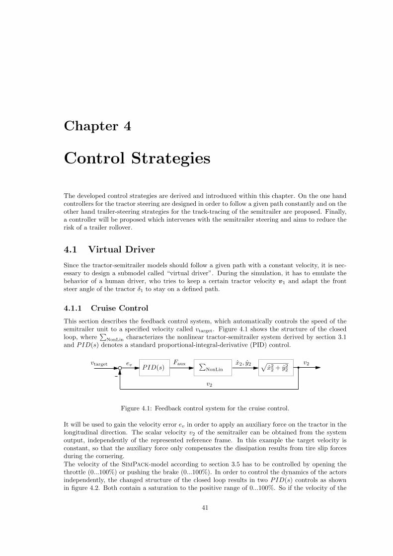
Chapter 4
Control Strategies
The developed control strategies are derived and introduced within this chapter. On the one handcontrollers for the tractor steering are designed in order to follow a given path constantly and on theother hand trailer-steering strategies for the track-tracing of the semitrailer are proposed. Finally,a controller will be proposed which intervenes with the semitrailer steering and aims to reduce therisk of a trailer rollover.
4.1 Virtual Driver
Since the tractor-semitrailer models should follow a given path with a constant velocity, it is nec-essary to design a submodel called “virtual driver”. During the simulation, it has to emulate thebehavior of a human driver, who tries to keep a certain tractor velocity v1 and adapt the frontsteer angle of the tractor δ1 to stay on a defined path.
4.1.1 Cruise Control
This section describes the feedback control system, which automatically controls the speed of thesemitrailer unit to a specified velocity called vtarget. Figure 4.1 shows the structure of the closedloop, where
∑NonLin characterizes the nonlinear tractor-semitrailer system derived by section 3.1
and PID(s) denotes a standard proportional-integral-derivative (PID) control.
vtarget v2PID(s)
∑NonLin
Faux √x2
2 + y22
x2, y2
v2
ev
Figure 4.1: Feedback control system for the cruise control.
It will be used to gain the velocity error ev in order to apply an auxiliary force on the tractor in thelongitudinal direction. The scalar velocity v2 of the semitrailer can be obtained from the systemoutput, independently of the represented reference frame. In this example the target velocity isconstant, so that the auxiliary force only compensates the dissipation results from tire slip forcesduring the cornering.The velocity of the SimPack-model according to section 3.5 has to be controlled by opening thethrottle (0...100%) or pushing the brake (0...100%). In order to control the dynamics of the actorsindependently, the changed structure of the closed loop results in two PID(s) controls as shownin figure 4.2. Both contain a saturation to the positive range of 0...100%. So if the velocity of the
41

42 4.1. Virtual Driver
vtarget v2PID(s)
∑SP
Throttle
√x2
2 + y22
x2, y2
v2
evBrake
PID(s)
−1
Figure 4.2: Feedback control system for the cruise control.
semitrailer is greater than the target velocity (ev < 0), the break will be pushed and the throttlewill be ignored.
Remark 4.1. Since the linear model derived in section 3.3 is derived with the assumption of aconstant body velocity, this control system is not necessary for simulating the linear system.
4.1.2 Tractors Steering Control
Before the design-process of a steering control for the front angle of the tractor, the definition ofthe target path has to be discussed. A path can be discretized by a number of path points. Theirinterconnection shapes a polygon, which describes a certain path. In order to generate varioustypes of paths, during this thesis the following functions are developed:
• pathAddStraight(...) → generate multiple points on a straight path;
• pathAddArc( radius,...) → generate multiple points on an arg path, specified by a given theradius;
• pathAddSin(...) → generate multiple points on a sine path.
A hypothetical created polygon of the so-called “target-path” is depicted in figure 4.3.The target steer angle of the tractor during each simulation time-step depends on the tractor’sposition, orientation and the given target path-polygon. So the strategy for the steering controlleris to detect and follow the path-polygon in the close environment of the tractor’s front, similarlyas it does a human.
-10 0 10 20 30 40 500
5
10
15
20
25
30
35
40
y/m
x/m
straight path
arc path
sine path
Figure 4.3: A hypothetical target-path polygon, defined by path points and created by developedthe functions.
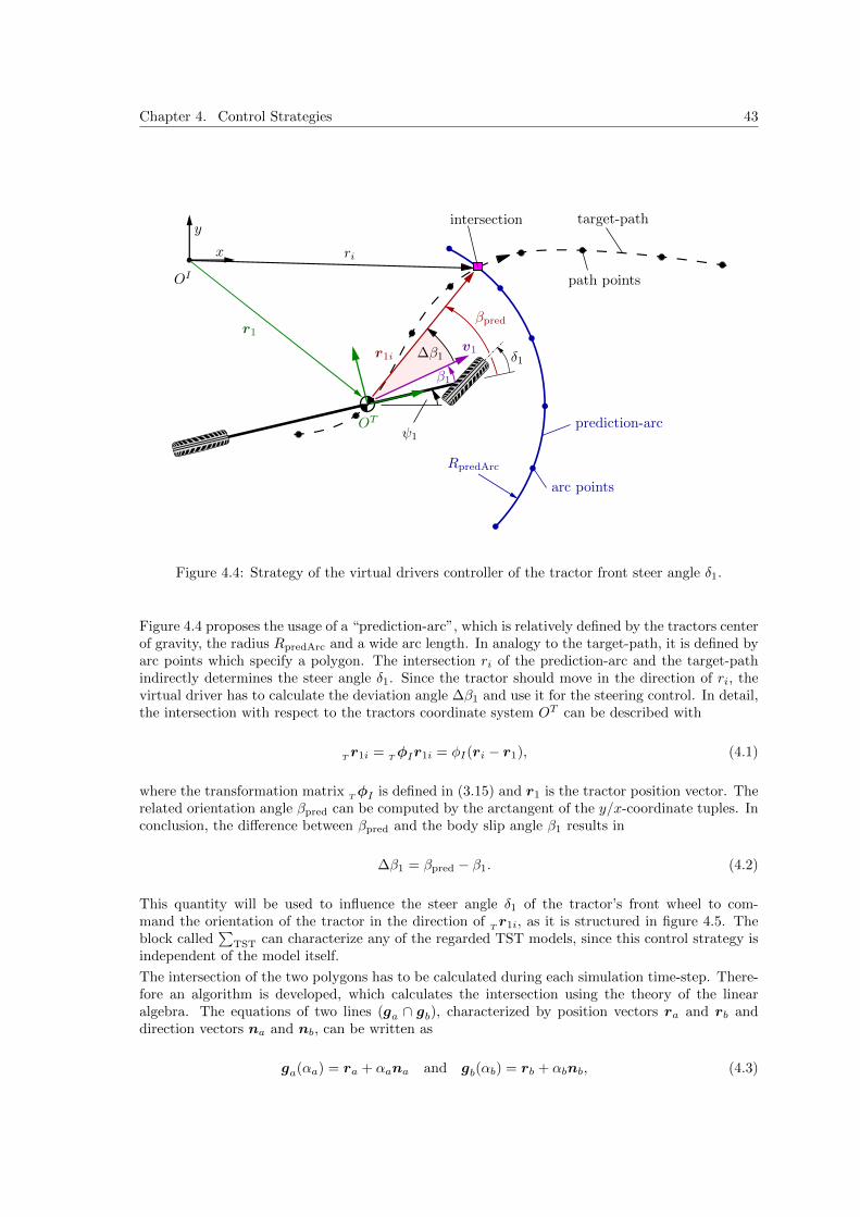
Chapter 4. Control Strategies 43
x
y
∆β1
OI
OT
r1
ψ1
β1
βpred
ri
v1r1i
prediction-arc
target-path
path points
arc points
RpredArc
intersection
δ1
Figure 4.4: Strategy of the virtual drivers controller of the tractor front steer angle δ1.
Figure 4.4 proposes the usage of a “prediction-arc”, which is relatively defined by the tractors centerof gravity, the radius RpredArc and a wide arc length. In analogy to the target-path, it is defined byarc points which specify a polygon. The intersection ri of the prediction-arc and the target-pathindirectly determines the steer angle δ1. Since the tractor should move in the direction of ri, thevirtual driver has to calculate the deviation angle ∆β1 and use it for the steering control. In detail,the intersection with respect to the tractors coordinate system OT can be described with
Tr1i =
TφIr1i = φI(ri − r1), (4.1)
where the transformation matrixTφI is defined in (3.15) and r1 is the tractor position vector. The
related orientation angle βpred can be computed by the arctangent of the y/x-coordinate tuples. Inconclusion, the difference between βpred and the body slip angle β1 results in
∆β1 = βpred − β1. (4.2)
This quantity will be used to influence the steer angle δ1 of the tractor’s front wheel to com-mand the orientation of the tractor in the direction of
Tr1i, as it is structured in figure 4.5. The
block called∑
TST can characterize any of the regarded TST models, since this control strategy isindependent of the model itself.
The intersection of the two polygons has to be calculated during each simulation time-step. There-fore an algorithm is developed, which calculates the intersection using the theory of the linearalgebra. The equations of two lines (ga ∩ gb), characterized by position vectors ra and rb anddirection vectors na and nb, can be written as
ga(αa) = ra + αana and gb(αb) = rb + αbnb, (4.3)

44 4.2. Steering Strategies for the Track-Tracing of a Semitrailer
target-path r1, ψ1∑TST
∆β1kPIntersection Trafo
Tri
arctan yx
βpred
prediction-arc
ri
β1
r1, ψ1
δ1
Figure 4.5: Feedback control system for the tractors steering control.
correct intersection
intersection will notbe taken into account
current consideredδ1path points (limited range)
Figure 4.6: Considered path point of the virtual driver are limited to a certain range.
where αa and αb are the line parameters. If the two lines intersect (ga!= gb), there will exist a
solution for the inhomogeneous linear system of equations in the form of[αaiαbi
]=[−na nb
]−1(ra − rb). (4.4)
Ensuring that the lines are only considered in the range between the polygon points, the position
vector r(k)a and direction vector n
(k)a has to be redefined for each intersection calculation at each
kth-polygon line part. If the parameters are in the range of
0 ≤ αai ≤ 1 and 0 ≤ αbi ≤ 1, (4.5)
the polygon intersection will result from (4.3) with
ri = r(k)a + αai n
(k)a . (4.6)
In some cases there exist additional intersections between the prediction-arc and previous or subse-quent target-path parts. This can be prevented with the consideration of path points in a limitedrange, starting at the recent path point, which took part for the previous calculation of the inter-section. Figure 4.6 shows these relations and also clarifies, that the paths are treated as a polygon.
4.2 Steering Strategies for the Track-Tracing of a Semitrailer
– THE CONFIDENTIAL CONTENT IS RESTRICTED –
4.2.1 Feedforward Controller for a Steady-State Turn
– THE CONFIDENTIAL CONTENT IS RESTRICTED –

Chapter 4. Control Strategies 45
4.2.2 Feed-Back Controller for a Path-Following
– THE CONFIDENTIAL CONTENT IS RESTRICTED –
4.2.3 Feedforward-Feedback Control (FFFB)
– THE CONFIDENTIAL CONTENT IS RESTRICTED –
4.2.4 FFFB with Reset & Patch-Strategy
– THE CONFIDENTIAL CONTENT IS RESTRICTED –
4.2.5 FFFB with Reset & Shift-Strategy
– THE CONFIDENTIAL CONTENT IS RESTRICTED –
4.2.6 FFFB with Relative Coordinates
– THE CONFIDENTIAL CONTENT IS RESTRICTED –
4.3 Steering Strategies for Active Rollover Avoidance
– THE CONFIDENTIAL CONTENT IS RESTRICTED –
4.3.1 Rollover of a Single-Unit Vehicle
– THE CONFIDENTIAL CONTENT IS RESTRICTED –
4.3.2 Active Roll Damping of a Tractor-Semitrailer
– THE CONFIDENTIAL CONTENT IS RESTRICTED –
46 4.3. Steering Strategies for Active Rollover Avoidance

Chapter 5
Simulation
The derived tractor-semitrailer (TST) models and steering strategies are implemented in differentsimulation software in order to analyze the system behavior for different drive maneuvers. Thischapter describes the simulation structures and results of the designed models and steering strate-gies.
5.1 Simulation Structure
Within the scope of this work various models and strategies are developed. This section gives abrief overview of the process chain and introduces the structures of the different simulation models.
5.1.1 Global Process Chain
Figure 5.1 shows the generalized process chain for the tractor-semitrailer simulation. The constantmodel parameters, simulation settings, controller parameters and initial conditions are definedduring the “Pre-Processing”. Furthermore the model inputs i.e. the tractor steer angle δ1 or targetpath are determined. The next step includes the calculation of the simulation results. On one hand,the derived nonlinear and linear TST-model equations are completely implemented in Simulinkand on the other hand the complex validation model runs in a “Co-Simulation dll-Interface” withSimPack. Afterwards the simulation results can be red and the trajectories can be calculated withrespect to the initial reference frame OI . The summary of the results is plotted in several figuresand a 3D-animation of the moving tractor-semitrailer can be generated. This animation is createdby the MATLAB-Toolbox “MatCarAnim”, which was developed in the scope of this thesis andis documented in the appendix B.
5.1.2 Structure of the Simulation Models
The following TST-models introduced in chapter 3 are considered and investigated in the scope ofthis thesis:
• Nonlinear Lateral-Yaw Model∑
TST
• Linear Lateral-Yaw Model∑
TST,lin
• SimPack-Model∑
TST,SP
• Nonlinear Lateral-Yaw-Roll Model∑
TST,Roll
• Linear Lateral-Yaw-Roll Model∑
TST,lin,Roll
At first the steering strategies for the track-tracing of the semitrailer will be analyzed using the“Lateral-Yaw Models” and the system structure according to figure 5.2. The equations of motionare implemented in the subsystem “Tractor-Semitrailer-Model” which is involved in the integra-tion loop. The state vector x includes the generalized coordinates q in state-space representation
47

48 5.1. Simulation Structure
conforming to equations (2.51) and (3.63), respectively. The model parameters are provided in astructure variable. Normally a human driver steers the tractor, opens the throttle and pushes thebrake. So during the simulation these tasks are managed by the “Virtual Driver” which needs thecurrent tractor position with respect to the initial reference frame and the system states. The cruisecontrol ensures that the TST drives with a target velocity. On one hand, it is possible to give atarget path which should be followed by the tractor and on the other hand the steer angle of thetractor can be directly defined. The track-tracing strategy of the semitrailer is implemented in theblock “Semitrailer Ctr (FFFB)” which contains the steady-state law and one of the path-followingcontrollers of the sections 4.2.2-4.2.6.
– THE CONFIDENTIAL CONTENT IS RESTRICTED –
The state vector xr includes the generalized coordinates qr in state-space representation again.The different constellation are analysed in the following section.
addPath(common used Functions & Toolboxes)
Initialize Struct with Model Parameters: par = set par(..)
Initialize Flags, Controller Parameters and Initial Conditions
Create “Target Path” or define the Tractor Steer Angle δ1 / Plot
Simulation / Integration of the Simulink-Modelsimat 8904 r2010a.dll SimPack-Model
Only for the Simulation of the SimPack-Model
MATLAB
Pre-P
rocessing
Read Simulink-Simulation Results
Calc & Plot Trajectories with respect to OI
3D-Animation with the developed Toolbox: MatCarAnim
MATLAB
Post-P
rocessing
Figure 5.1: Structure of the global process chain for the tractor-semitrailer simulation.

Chapter 5. Simulation 49
vtarget
∑TST
x
δ1
δ2
Throttle/
x
Integration Loop
∫Brake
Ftires
Tractor-Semitrailer-Model
Virtual Driver
Cruise-Ctr
δ1-Ctr
User-def. δ1
x
∑FB
∑FF
δ2
dmeasurement: Γ,˙ψ2, S v2
Ftires
noise
mea
sura
ble
state
s
Semitrailer Ctr (FFFB)
δ1
x Faux
Tractor Position
r1 = [x1; y1]T[x1 y1] = f(x)
Target Path
state vector x
ModelParameters
par
Figure 5.2: Simulation structure of the lateral-yaw models for the investigation of the track-tracing.
5.2 Results and Analysis
This chapter presents and analysis the simulation results of the concerning simulation models andstrategies. Beside the validation of the various TST-models, the impacts of steering strategies andthe behaviors of the dynamic systems are analyzed. The explicit values of the model parametersand control gains are given in the appendix A.1.
5.2.1 Response Characteristics of the linear Models
The system-dynamics of the linear “Lateral-Yaw Model” (∑
TST,lin) and “Lateral-Yaw-Roll Model”(∑
TST,lin,Roll) can be characterized by multiple transfer functions. They can be formulated fromeach input to each output and are defined by a single regarded Laplace transferred input U(s) andoutput Y (s). In general it results in
Gyu(s) :=Y (s)
U(s). (5.1)
For a system in state-space representation it can be calculated according to (2.56). Initially themodel
∑TST,lin has to be taken into account. One consideration is the influence of the semitrailer
steer angle δ2 on the yaw dynamics (i.e. ψ2) of the trailer. According to (3.71) the previous transferfunction results in
Gψ2δ2(s) = cT
ψ2(sI −A)−1bδ2 . (5.2)
The input matrix bδ2 is the second column of B from equation (3.71) and the output matrix is therow vector cψ2
=[0 0 0 1
], which is used to select the semitrailer yaw velocity ψ2. Figure 5.3
depicts the Bode-diagram for various TST velocities. It shows that the magnitude of the responseexponentially increases with velocity and that a velocity of more than 120km/h leads to highamplifications(|Gψ2δ2
| > 1) at frequencies between 1rad/s and 10rad/s.

50 5.2. Results and Analysis
The transfer function from the semitrailer steer angle δ2 to the roll angular velocity (i.e. φ2) ofthe trailer can be calculated in order to investigate the roll dynamics of the semitrailer. It can bederived from equation (3.106) with
Gφ2δ2(s) = cT
rφ2(sI −Ar)
−1brδ2 . (5.3)
Similarly the input matrix brδ2 is the second column of Br from equation (3.106) and the outputmatrix is the row vector cφ2
=[0 0 0 0 0 0 1 0
], which is used to select the semitrailer
roll velocity φ2. Figure 5.4 illustrates the Bode-diagram of the roll transfer function for differentTST velocities. It also shows that the magnitude of the response exponentially increases with thevelocity and that a velocity of more than 120km/h leads to high roll amplifications(|Gφ2δ2
| > 1) atfrequencies between 2rad/s and 8rad/s.
5.2.2 Validation of the TST-Models
The various TST-models must be validated and compared before they can be used for the assessmentof the steering strategies. For the general validation of the models the steering the semitrailer isignored which means δ2 = 0. Figure 5.5 depicts the animation screen-shots of a TST entering aroundabout. The simulation results were calculated with the “Nonlinear Lateral-Yaw Model”
∑TST
and the animation was created with the Toolbox MatCarAnim. Figure 5.5(a) clarifies the single-track model in a 3D-view and figure 5.5(b) shows it from a top-view. Furthermore, the trajectoriesof the 5th-wheel and the rearmost trailer end are illustrated. Since the trailer is unsteered it offtracksto the inside of the turns, which results in a deviation of the both trajectories. Within this drivingmaneuver the different models are compared and validated in the following.
-40
-30
-20
-10
0
10
|Gψ
2δ2(jω
)|/
dB
10−290
180
270
360
Ph
ase
/d
eg
Frequency ω (rad/s)
v = 15km/h
v = 30km/h
v = 60km/h
v = 120km/h
10−1 100 101 102 103
Figure 5.3: Bode diagram of the amplitude frequency response Gψ2δ2(jω) of the yaw transfer
function at different TST velocities.
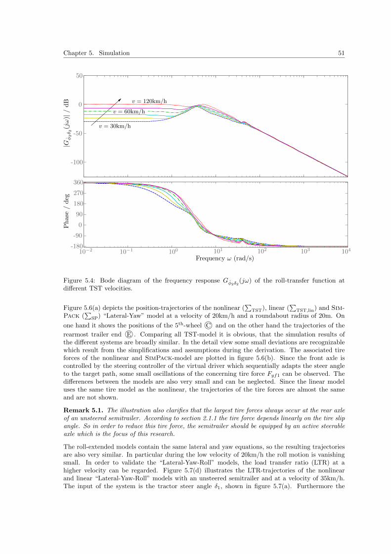
Chapter 5. Simulation 51
-100
-50
0
50
|Gφ2δ2(jω
)|/
dB
v = 30km/h
v = 60km/h
-180
-90
0
90
180
270
360
Ph
ase
/d
eg
10−2
Frequency ω (rad/s)10−1 100 101 102 103 104
v = 120km/h
Figure 5.4: Bode diagram of the frequency response Gφ2δ2(jω) of the roll-transfer function at
different TST velocities.
Figure 5.6(a) depicts the position-trajectories of the nonlinear (∑
TST), linear (∑
TST,lin) and Sim-Pack (
∑SP) “Lateral-Yaw” model at a velocity of 20km/h and a roundabout radius of 20m. On
one hand it shows the positions of the 5th-wheel jC and on the other hand the trajectories of the
rearmost trailer end jE . Comparing all TST-model it is obvious, that the simulation results ofthe different systems are broadly similar. In the detail view some small deviations are recognizablewhich result from the simplifications and assumptions during the derivation. The associated tireforces of the nonlinear and SimPack-model are plotted in figure 5.6(b). Since the front axle iscontrolled by the steering controller of the virtual driver which sequentially adapts the steer angleto the target path, some small oscillations of the concerning tire force Fyf1 can be observed. Thedifferences between the models are also very small and can be neglected. Since the linear modeluses the same tire model as the nonlinear, the trajectories of the tire forces are almost the sameand are not shown.
Remark 5.1. The illustration also clarifies that the largest tire forces always occur at the rear axleof an unsteered semitrailer. According to section 2.1.1 the tire force depends linearly on the tire slipangle. So in order to reduce this tire force, the semitrailer should be equipped by an active steerableaxle which is the focus of this research.
The roll-extended models contain the same lateral and yaw equations, so the resulting trajectoriesare also very similar. In particular during the low velocity of 20km/h the roll motion is vanishingsmall. In order to validate the “Lateral-Yaw-Roll” models, the load transfer ratio (LTR) at ahigher velocity can be regarded. Figure 5.7(d) illustrates the LTR-trajectories of the nonlinearand linear “Lateral-Yaw-Roll” models with an unsteered semitrailer and at a velocity of 35km/h.The input of the system is the tractor steer angle δ1, shown in figure 5.7(a). Furthermore the
52 5.3. Figures
tire forces (calculated by a saturated tire force law) are depicted in figure 5.7(b). Finally theposition-trajectories are shown in figure 5.7(c). Since the TST drives with a high velocity and arelatively large tractor steer angle is applied, the rear tire force of the semitrailer is saturated andthe semitrailer is close to a rollover (LTR2 → 1). The difference between the nonlinear (
∑TST,Roll)
and linear (∑
TST,lin,Roll) roll-extended model is very small, so it can be assumed that the linearmodel is valid and accurate for the roll investigations.
5.2.3 Track-Following Analysis with the Horizontal Planar Models
– THE CONFIDENTIAL CONTENT IS RESTRICTED –
5.2.4 Active-Roll-Damping Analysis with the Roll-extended Models
– THE CONFIDENTIAL CONTENT IS RESTRICTED –
5.3 Figures
This section contains the essential figures of the simulation results. For simulating a time of 20sec,the calculation times approximately resulted:
• Nonlinear-models: about 20 sec
• Linear-model: about 10 sec
• SimPack-model: about 2 min
– THE CONFIDENTIAL CONTENT IS RESTRICTED –

Chapter 5. Simulation 53
(a) 3D view of the TST
(b) Top view of the TST
x/m
−x/m
y/m
y/m
5th-wheel: jCreasmost trailer end: jE
Trajectory of the road
Trajectory
of the road
Figure 5.5: Animation of a tractor with an unsteered semitrailer entering a roundabout. The sim-ulation results were calculated with the “Nonlinear Lateral-Yaw Model”
∑TST and the animation
was created with the Toolbox MatCarAnim.

54 5.3. Figures
30 40 50 60 70 80
0
5
10
15
20
25
30
35
40
x / m
y/
m
4 6 8 10 12 14 16 18 20
-4
-3
-2
-1
0
1
2
3
4
×104
t/s
Fti
res
/m
∑TST∑SP
Fyr2
Fyf2
Fyr1
Fym2Fyf1
∑TST∑TST,lin∑SP
rearmost trailer end: jE
5th-wheel: jC
(b) Tire forces of the tractor with the unsteered semitrailer (Nonlinear & SimPack-model).
(a) Trajectories of 5th-wheel and rear trailer end position (Nonlinear, Linear & SimPack-model).
jE
jC
Detail
Figure 5.6: Position-trajectories of the different models with an unsteered semitrailer and at avelocity of 20km/h.

Chapter 5. Simulation 55
0 2 4 6 8 10 12 14 16 18-10
0
10
t / s
δ 1/
deg
0 2 4 6 8 10 12 14 16 18-8
-6
-4
-2
0
2
4
6
8×10⁴
t / s
Fti
res
/N
-20 0 20 40 60 800
20
40
60
80
x /m
y/m
0 2 4 6 8 10 12 14 16 18-1
-0.8
-0.6
-0.4
-0.2
0
0.2
0.4
0.6
0.8
1
t / s
LT
R1
<
R2
(a) Tractor steer angle
(b) Tire Forces
(c) Position trajectories
(d) Load transfer ratio (LTR)
Fyr2
Fyf2
Fym2Fyf1
Fyf1
∑TST,Roll∑TST,lin,Roll
LTR2: Semitrailer
LTR1: Tractor
Figure 5.7: Trajectories of the nonlinear and linear “Lateral-Yaw-Roll” models with an unsteeredsemitrailer and at a velocity of 35km/h.

56 5.3. Figures

Chapter 6
Summary and Outlook
This thesis focuses the modeling and control of articulated tractor-semitrailers (TST). StandardEuropean semitrailers usually utilize an unsteered tri-axle group. They are produced with lowfinancial efforts but have a high tire wear and a reduced maneuverability. The objective of thisthesis was to investigate the utilization of a steered rearmost axle of semitrailers in order to improvethe performance during low-speed turning maneuvers, high-speed cornering and to react duringcritical situations such as rollover.The second chapter introduced some fundamentals of vehicle dynamics with respect to the charac-terization of the tires, basic vehicle modeling and TST specific approaches. Furthermore, insightsof previous research were given and some existing steering and control strategies for a tractor-semitrailer trace-tracking and rollover prevention were presented.The first challenge during this work was to derive a linear and nonlinear TST single-track model,which take the lateral and yaw motion of the coupled vehicles into account. On the one hand thenonlinear equations of motion (derived by the Newton-Euler approach) characterize the dynamicbehavior very accurately, but on the other hand the simplified linear equations can be used forsystem analysis and for the design of linear model-based controls. The linear model was representedwith a saturated tire model and as a fully linear formulation. In addition, the models were extendedand re-derived in order to account for the roll motions of the system at high-speed. Finally, theexisting multibody simulation (SimPack) model was introduced.Afterwards the control strategies for the tractor front axle steering and the semitrailer rearmostaxle steering were developed and explained. Since the main focus of this thesis was to improvethe semitrailer tracking and roll behavior using rear axle steering, multiple control strategies forthe semitrailer-steering were designed. Thereby the trajectory of the coupling point is traced withthe rear trailer end, reducing offtrack and improving maneuverability of the vehicle. In this scopea steady-state and feedback control strategy was developed. In addition, a feedforward-feedbackcontroller (FFFB) combines both strategies. Furthermore an “active rollover damping”(ARD)control law was proposed, which intervenes with the tractor and / or the trailer steering and aimsto reduce the risk of a trailer rollover.Finally, the derived models and controllers were implemented into the simulation environments. Theprocess chain and simulation structures were illustrated and explained. The models were validatedand compared within the simulation results. The influences and improvements of the steeringstrategies were investigated for a typical maneuver: entering a roundabout at low velocity. It wasshown that the FFFB strategy leads to a reliable track-tracing at both, the simplified nonlinearTST model and the precise SimPack model. Moreover the ARD was tested at the tractor and thesemitrailer steering. The roll dynamics were simulated during a critical maneuver and the resultswere analyzed.
– THE CONFIDENTIAL CONTENT IS RESTRICTED –
In a further research the derived TST models can be used in order to extend the investigation and
57
58
improvement of the model dynamics using the trailer steering. An optimal path following behaviorof the trailer can probably also be realized, designing appropriate observers. The introduced activeroll damping strategy is very simple, has a great potential and should be considered in furtherinvestigations. Of course, new alternative rollover-prevention-controls could also lead to muchbetter improvements. However, before an universal steering strategy can be implemented on a realsemitrailer control device, various control and switching strategies for mixed maneuver (low andhigh speed / sharp and smooth cornering / different load cases) should be designed and testedintensively.
Appendix A
Model Parameters and AdditionalDerivations
A.1 Vehicle Parameters
– THE CONFIDENTIAL CONTENT IS RESTRICTED –
A.2 Math Notations
This chapter introduces the math notations of this work. On one hand they are inducted tosimplify and shorten the equations and on the other hand they should be conductive to the clearunderstanding of complex relations.In expensive equations the trigonometric functions of an arbitrary angle α are abbreviated with
sα = sin(α) cα = cos(α), (A.1)
as it was suggested in [PS10]. Whenever a symbol of the Greek alphabet is sub-scripted after a ’s’or ’c’ letter, it will be treated as the argument of the sinus or cosines function, respectively.If a vector r or coordinate tuple x is expressed with respect to a reference frame called OS , theabbreviation will be subscripted before the quantity,
Sr , or
Sx. (A.2)
Otherwise they are related to the initial reference frame OI . Furthermore the transformation of areference frame OT to the frame OS will be notated with
SφT . (A.3)
The description of a trajectory or discrete points of time will be realized with a super-scripted andstapled index or position. So a position trajectory of n values can be exemplarily described by
r(k), where k = 1(1)n. (A.4)
A.3 Equations of Motion according to the Lagrangian Ap-proach
In the following, the non-linear model in agreement with the Lagrangian equations of motion ofsecond kind is derived. In [dB01] and [FMG06] a model of an articulated vehicle with n-trailers
59

60 A.3. Equations of Motion according to the Lagrangian Approach
conforming to Lagrange’s method was established. The kinematic energy (T ) can be written as
T =1
2
2∑k=1
[˙rTk ψk
]Mk
[rTk ψk
]T(A.5)
where rk is the position vector of the center of gravity and Mk denotes the mass matrix
Mk =
mk 0 00 mk 00 0 Ik
(A.6)
of the corresponding body with index k. With the determination of the generalized coordinates
q =[x2 y2 ψ2 ψ1
]T, (A.7)
the vector[rTk ψk
]Tcan be expressed by[
rkψk
]= Jk q , (A.8)
where J1 is the Jacobian matrix of the tractor and J1 of the semitrailer body,
J1 =
1 0 −b1 sinψ2 −l2 sinψ1
0 1 b1 cosψ2 l2 cosψ1
0 0 0 1
and J2 =
1 0 0 00 1 0 00 0 1 0
. (A.9)
Substituting (A.8) into (A.5) yields
T =1
2qT M(q) q , where M(q) =
2∑k=1
JTk Mk Jk (A.10)
is the global mass matrix. In contrast to the matrix presentation, the kinetic energy can also becalculated segmentally,
T =1
2
2∑k=1
2∑l=1
M[k,l] q[k] q[l] . (A.11)
According to the methods of the virtual work described in [Sha05], the D’Alembert-Lagrange’sequation can be derived. For the current MBS with four degree of freedoms it results
4∑i=1
(d
dt
∂T
∂q[i]− ∂T
∂q[i]−Q[i]
)δq[i] = 0 , (A.12)
where δq is the vector of virtual displacement in generalized coordinates and Q is the vector ofgeneralized forces, respectively, the term
∑4i=1Q[i] δq[i] characterise the virtual work δWe of the
generalized forces. It can also be calculated with the vector of applied forces F e and the virtualdisplacement δre in Cartesian coordinates in matrix form,
δWe = QT δq = F Te δre . (A.13)
Since the virtual displacement in Cartesian coordinates can be written as
δre =∂re∂q
δq , (A.14)
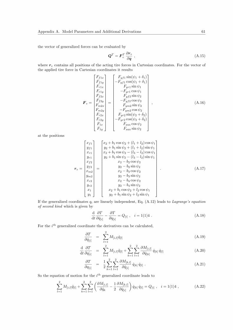
Appendix A. Model Parameters and Additional Derivations 61
the vector of generalized forces can be evaluated by
QT = F Te∂re∂q
, (A.15)
where re contains all positions of the acting tire forces in Cartesian coordinates. For the vector ofthe applied tire force in Cartesian coordinates it results
F e =
Ff1x
Ff1y
Fr1xFr1yFf2x
Ff2y
Fm2x
Fm2y
Fr2xFr2yF1x
F1y
=
Fyf1 sin(ψ1 + δ1)−Fyf1 cos(ψ1 + δ1)
Fyr1 sinψ1
−Fyr1 cosψ1
Fyf2 sinψ2
−Fyf2 cosψ2
Fym2 sinψ2
−Fym2 cosψ2
Fyr2 sin(ψ2 + δ2)−Fyr2 cos(ψ2 + δ2)
Faux cosψ2
Faux sinψ2
, (A.16)
at the positions
re =
xf1
yf1
xr1yr1xf2
yf2
xm2
ym2
xr2yr2x1
y1
=
x2 + b1 cosψ2 + (l1 + l2) cosψ1
y2 + b1 sinψ2 + (l1 + l2) sinψ1
x2 + b1 cosψ2 − (l3 − l2) cosψ1
y2 + b1 sinψ2 − (l3 − l2) sinψ1
x2 − b2 cosψ2
y2 − b2 sinψ2
x2 − b3 cosψ2
y2 − b3 sinψ2
x2 − b4 cosψ2
y2 − b4 sinψ2
x2 + b1 cosψ2 + l2 cosψ1
y2 + b1 sinψ2 + l2 sinψ1
. (A.17)
If the generalized coordinates qi are linearly independent, Eq. (A.12) leads to Lagrange’s equationof second kind which is given by
d
dt
∂T
∂q[i]− ∂T
∂q[i]= Q[i] , i = 1(1)4 . (A.18)
For the ith generalized coordinate the derivatives can be calculated,
∂T
∂q[i]=
2∑l=1
M[i,l]q[l] (A.19)
d
dt
∂T
∂ ˙q[i]=
2∑l=1
M[i,l]q[l] +
2∑k=1
2∑l=1
∂M[i,l]
∂q[k]q[k] q[l] (A.20)
∂T
∂q[i]=
1
2
2∑k=1
2∑l=1
∂M[k,l]
∂q[i]q[k] q[l] . (A.21)
So the equation of motion for the ith generalized coordinate leads to
2∑l=1
M[i,l]q[l] +
2∑k=1
2∑l=1
(∂M[i,l]
∂qk− 1
2
∂M[k,l]
∂q[i]
)q[k] q[l] = Q[i] , i = 1(1)4 , (A.22)
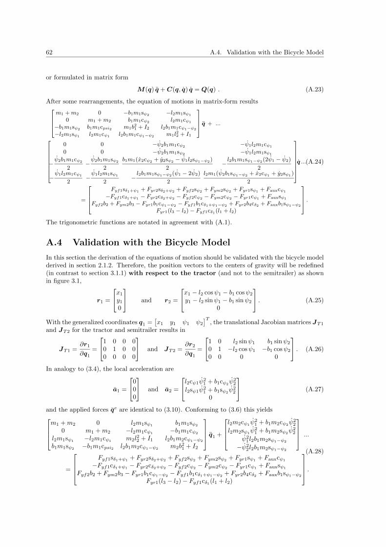
62 A.4. Validation with the Bicycle Model
or formulated in matrix form
M(q) q +C(q, q) q = Q(q) . (A.23)
After some rearrangements, the equation of motions in matrix-form resultsm1 +m2 0 −b1m1sψ2 −l2m1sψ1
0 m1 +m2 b1m1cψ2 l2m1cψ1
−b1m1sψ2 b1m1cpsi2 m1b21 + I2 l2b1m1cψ1−ψ2
−l2m1sψ1 l2m1cψ1 l2b1m1cψ1−ψ2 m1l22 + I1
q + ...
0 0 −ψ2b1m1cψ2 −ψ1l2m1cψ1
0 0 −ψ2b1m1sψ2 −ψ1l2m1sψ1
−ψ2b1m1cψ2
2−ψ2b1m1sψ2
2
b1m1(x2cψ2 + y2sψ2 − ψ1l2sψ1−ψ2)
2−l2b1m1sψ1−ψ2(2ψ1 − ψ2)
2
−ψ1l2m1cψ1
2−ψ1l2m1sψ1
2−l2b1m1sψ1−ψ2(ψ1 − 2ψ2)
2
l2m1(ψ2b1sψ1−ψ2 + x2cψ1 + y2sψ1)
2
q ...
=
Fyf1sδ1+ψ1 + Fyr2sδ2+ψ2 + Fyf2sψ2 + Fym2sψ2 + Fyr1sψ1 + Fauxcψ1
−Fyf1cδ1+ψ1 − Fyr2cδ2+ψ2 − Fyf2cψ2 − Fym2cψ2 − Fyr1cψ1 + Fauxsψ1
Fyf2b2 + Fym2b3 − Fyr1b1cψ1−ψ2 − Fyf1b1cδ1+ψ1−ψ2 + Fyr2b4cδ2 + Fauxb1sψ1−ψ2
Fyr1(l3 − l2) − Fyf1cδ1(l1 + l2)
.
(A.24)
The trigonometric functions are notated in agreement with (A.1).
A.4 Validation with the Bicycle Model
In this section the derivation of the equations of motion should be validated with the bicycle modelderived in section 2.1.2. Therefore, the position vectors to the centers of gravity will be redefined(in contrast to section 3.1.1) with respect to the tractor (and not to the semitrailer) as shownin figure 3.1,
r1 =
x1
y1
0
and r2 =
x1 − l2 cosψ1 − b1 cosψ2
y1 − l2 sinψ1 − b1 sinψ2
0
. (A.25)
With the generalized coordinates q1 =[x1 y1 ψ1 ψ2
]T, the translational Jacobian matrices JT1
and JT2 for the tractor and semitrailer results in
JT1 =∂r1
∂q1
=
1 0 0 00 1 0 00 0 0 0
and JT2 =∂r2
∂q1
=
1 0 l2 sinψ1 b1 sinψ2
0 1 −l2 cosψ1 −b1 cosψ2
0 0 0 0
. (A.26)
In analogy to (3.4), the local acceleration are
a1 =
000
and a2 =
l2cψ1ψ21 + b1cψ2
ψ22
l2sψ1ψ21 + b1sψ2
ψ22
0
(A.27)
and the applied forces qe are identical to (3.10). Conforming to (3.6) this yieldsm1 +m2 0 l2m1sψ1
b1m1sψ2
0 m1 +m2 −l2m1cψ1−b1m1cψ2
l2m1sψ1 −l2m1cψ1 m2l22 + I1 l2b1m2cψ1−ψ2
b1m1sψ2 −b1m1cpsi2 l2b1m2cψ1−ψ2 m2b21 + I2
q1 +
l2m2cψ1
ψ21 + b1m2cψ2
ψ22
l2m2sψ1ψ2
1 + b1m2sψ2ψ2
2
ψ21l2b1m2sψ1−ψ2
−ψ22l2b1m2sψ1−ψ2
...
=
Fyf1sδ1+ψ1
+ Fyr2sδ2+ψ2+ Fyf2sψ2
+ Fym2sψ2+ Fyr1sψ1
+ Fauxcψ1
−Fyf1cδ1+ψ1 − Fyr2cδ2+ψ2 − Fyf2cψ2 − Fym2cψ2 − Fyr1cψ1 + Fauxsψ1
Fyf2b2 + Fym2b3 − Fyr1b1cψ1−ψ2 − Fyf1b1cδ1+ψ1−ψ2 + Fyr2b4cδ2 + Fauxb1sψ1−ψ2
Fyr1(l3 − l2)− Fyf1cδ1(l1 + l2)
.
(A.28)

Appendix A. Model Parameters and Additional Derivations 63
After the transformation (3.17) with the generalized coordinatesTq1 =
[Tx1 T
y1 ψ1 ψ2
]Tand the rotation matrix
x1
y1
ψ1
ψ2
︸ ︷︷ ︸q1
=
cosψ1 − sinψ1 0 0sinψ1 cosψ1 0 0
0 0 1 00 0 0 1
︸ ︷︷ ︸
IΦT
Tx1
Ty1
ψ1
ψ2
︸ ︷︷ ︸Tq1
(A.29)
to the tractor-fixed reference frame OT shown in figure 3.2, the tractor related equations of motioncan be written by
m1 +m2 0 0 −b1m2sψ1−ψ2
0 m1 +m2 −l2m2 −b1m2cψ1−ψ2
0 −l2m2 m2l22 + I1 l2b1m1cψ1−ψ2
−b1m2sψ1−ψ2 −b1m2cψ1−ψ2 l2b1m1cψ1−ψ2 m2b21 + I2
T q1+
ψ2
1l2m2 +ψ22b1m2cψ1−ψ2−ψ1 T y1(m1+m2)
−ψ21b1m2sψ1−ψ2 + ψ1 T x1(m1 +m2)
−l2m2(ψ1 T x1 − ψ22b1sψ1−ψ2)
−ψ1b1m2(T x1cψ1−ψ2+(ψ1l2 −T y1)sψ1−ψ2)
...
=
Faux + Fyr2sδ2−ψ1+ψ2 + Fyf1sδ1 − Fyf2sψ1−ψ2 − Fym2sψ1−ψ2
−Fyr1 − Fyr2cδ2−ψ1+ψ2 − Fyf1cδ1 − Fyf2cψ1−ψ2 − Fym2cψ1−ψ2
Fyr1l3 + Fyf2l2cψ1−ψ2 + Fym2l2cψ1−ψ2 + Fyr2l2cδ2−ψ1+ψ2 − Fyf1l1cδ1Fyf2(b1 + b2) + Fym2(b1 + b3) + Fyr2cδ2(b1 + b4)
.
(A.30)
If one consider the tractor vehicle without the trailer (m2 = Fyf2 = Fym2 = Fyr2 = 0) and theauxiliary force (Faux = 0), the simplified equation leads to
m1 0 0 00 m1 0 00 0 I1 00 0 0 0
Tq1 +
−ψ1 T y1m1
ψ1 T x1m1
00
=
Fyf1sδ1
−Fyf1cδ1 − Fyr1−Fyf1l1cδ1 + Fyr1l3
0
, (A.31)
respectively with (2.13) and the assumption of small steer angles δ1 << 1 it yields
m1 T x1 −m1ψ1 T y1 = Cαf αf δ1 (A.32)
m1 T y1 +m1ψ1 Tx1 = −Cαf αf − Cαr αr (A.33)
I1ψ1 = −Cαf αf l1 + Cαr αr l3 . (A.34)
The resulted velocity v1 and the body slip angle β1 of the tractor are depict in figure (A.1). They
Ty1
Tx1
β1
v1
Figure A.1: Explanation of β1, the body slip angle of the tractor.
are linked to the velocity components (Tx1, T y1) and with the assumption of a small body slip
angle β1 << 1 (equivalent to section 2.1.2) the following conditions can be derived,
cosβ1 = Tx1
v1≈ 1 ⇔
Tx1 ≈ v1 ⇒
Tx1 ≈ v1 (A.35)
sinβ1 = Ty1
v1≈ β1 ⇔
Ty1 ≈ v1β1 ⇒
Ty1 ≈ v1β1 + v1β1 . (A.36)

64 A.5. Alternative Derivation of the linear TST Model
In analogy to (2.16), the front and rear tire slip angles can be calculated by
αf ≈ δ1 −ψ1lfv1− β1 and αr ≈
ψ1lrv1− β1 . (A.37)
The next step is to insert the equations (A.35-A.37) in (A.32-A.34), which yields
m1v1 −m1ψ1v1β1 = Cαf
(δ1 −
ψ1lfv1− β1
)δ1 (A.38)
m1(v1β1 + v1β1) +m1ψ1v1 = −Cαf
(δ1 −
ψ1lfv1− β1
)− Cαr
(ψ1lrv1− β1
)(A.39)
I1ψ1 = −Cαf
(δ1 −
ψ1lfv1− β1
)l1 + Cαr
(ψ1lrv1− β1
)l3 . (A.40)
For a consideration of the vehicle at constant velocity (v = 0), the second and third equations leadsagain to the Riekert and Schunck’s equations (2.23)
m1v1(β1 + ψ1)− (Cαf + Cαr)β1 −Cαf l1 − Cαr l3
v1ψ1 = −Cαf δ1 (A.41)
I1ψ1 −1
v1(l23Cαr + l21Cαf ) ψ1 − (l1Cαf − l3Cαr)β1 = −Cαf δ1 l1 . (A.42)
A.5 Alternative Derivation of the linear TST Model
This section describes an alternative derivation of the linear tractor-semitrailer (TST) model. Theequations of motion derived in section 3.3 are obtained by simplifying and linearising the nonlinearTST model. In contrast, the linear model also directly results from a simplified approach of thetranslational and angular momentum. For of a body with the mass mi, the directional and lateralacceleration xi and yi, the moment of inertia Ii and the rotational acceleration ψi, it can be generallyformulated
mixi =∑
Fxi , miyi =∑
Fyi , and Iiψi =∑
Mi , (A.43)
where∑Fxi,
∑Fxi and
∑Mi characterize the forces and moment acting on the body. Figure A.2
shows the forces acting on the TST. In order to derive linear equations of motion, which describe
Γl1
l3
b1
l2b2
b3
b4
m2
m1
I1
δ1
δ2
Fyr1
Fyf1
Fyr2Fym2 Fyf2
x
y
OI
I2
ψ2v
ψ1v
β2
β1
Fc
Fc
Figure A.2: Single Track Model of Tractor and Semitrailer(TST) with a steered rearmost axle forthe derivation of the linear equations.
the lateral and rotational behavior of the TST, the simplifications reported by the enumeration in
Appendix A. Model Parameters and Additional Derivations 65
section 3.3 have to be taken into account. The lateral acceleration of the tractor can be describedby the body angular velocity ψ1, the change of the body slip angle β1 and the constant tractorvelocity v with
y1 = v(ψ1 + β1) . (A.44)
So the equilibrium of the forces in the direction of y (lateral) and the momentum around the c.g.of the tractor with the mass m1 and moment of inertia I1 yields
m1v(ψ1 + β1) = −Fyf1 − Fyr1 + Fc =Yβ1β1 + Yψ1ψ1 + Yδ1δ1 + Fc (A.45)
I1ψ1 = −Fyf1l1 + Fyr1l3 − Fc l2 =Nβ1β1 +Nψ1
ψ1 +Nδ1δ1 − Fc l2 , (A.46)
where the force Fc represents the internal force at the hitch. The tire forces at the front and rearwheel, Fyf1 and Fyr1, can also be linearly described by the terms Yβ1
, Yψ1and Yδ1 , the caused
torsional moment by Nβ1, Nψ1
and Nδ1 . Their explicit calculation will be explained later on.In analogy, the equations for the semitrailer can be written
m2v(ψ2 + β2) = −Fyf2 − Fyr2 − Fyr1 − Fc =Yβ2β2 + Yψ2
ψ2 + Yδ2δ2 − Fc (A.47)
I2ψ2 = Fyf2b2 + Fym2b3 + Fyr2b4 − Fcb1 =Nβ2β2 +Nψ2
ψ2 +Nδ2δ2 − Fcb1 . (A.48)
The internal hitch force Fc can either be eliminated by using (A.45) and (A.47),
m2v(ψ2 + β2) = Yβ2β2 + Yψ2
ψ2 + Yδ2δ2 −m1v(ψ1 + β1) + Yβ1β1 + Yψ1
ψ1 + Yδ1δ1 , (A.49)
or by using (A.45) and (A.48),
I2ψ2 = Nβ2β2 +Nψ2ψ2 +Nδ2δ2 −m1v(ψ1 + β1)b1 + Yβ1β1b1 + Yψ1
ψ1b1 + Yδ1δ1b1 , (A.50)
or in conclusion by using (A.45) and (A.46),
I1ψ1 = Nβ1β1 +Nψ1
ψ1 +Nδ1δ1 −m1v(ψ1 + β1)l2 + Yβ1β1l2 + Yψ1
ψ1l2 + Yδ1δ1l2 . (A.51)
The body slip angle of the tractor β1 and the slip angular velocity β1 can be substituted using thekinematic coupling constraints (3.37) and (3.38). Moreover, the derivation of (3.19) with respectto the time leads to the additional equation
Γ = ψ1 − ψ2 . (A.52)
Furthermore, the generalized coordinates
qlin =[Γ ψ1 β2 ψ2
]T(A.53)
and the input vector
u =[δ1 δ2
]T(A.54)
will be defined. After some rearrangements, the equations (A.51)-(A.52) can be written in matrixform as

66A
.5.
Alt
ernati
ve
Der
ivat
ion
ofth
eli
nea
rT
ST
Mod
el
0 m1l2 (m1 +m2)v m1b10 m1l2b1 m1b1v m1b
21 + I2
0 m1l22 + I1 m1l2v m1l2b1
1 0 0 0
qlin +
Yβ1 −Yψ1
− Yβ1l2v
−Yβ2 − Yβ1 (m1 +m2)v − Yψ2− Yβ1
b1v
Yβ1b1 −(Yψ1+ Yβ1
l2v
)b1 −Nβ2 − Yβ1b1 m1vb1 −Nψ2 − Yβ1b21v
Nβ1 + Yβ1 l2 −Nψ1−Yψ1l2−Yβ1
l22v−Nβ1
l2v
−Nβ1 − Yβ1 l2 m1l2v − (Nβ1 + Yβ1 l2) b1v
0 −1 0 1
qlin
... =
Yδ1 Yδ2Yδ1b1 Nδ2
Nδ1 + Yδ1 l2 00 0
u ,
(A.55)
which is equal to (3.65). The explicit linear model equations0 m1l2 (m1 +m2)v m1b10 m1l2b1 m1b1v m1b
21 + I2
0 m1l22 + I1 m1l2v m1l2b1
1 0 0 0
︸ ︷︷ ︸
˜M
qlin + ...
Cf1 + Cr1 Cr1
l3−l2v
− Cf1l1+l2v
− (Cf2 + Cm2 + Cr2 + Cf1 + Cr1) (m1+m2)v +Cf2b2v
+Cm2b3v
+Cr2b4v−(Cf1+Cr1) b1
v
Cf1b1 + Cr1b1 Cr1b1l3−l2v
− Cf1b1l1+l2v
Cf2b2+Cm2b3+Cr2b4−Cr1b1−Cf1b1 m1vb1 − Cf2b22v− Cm2
b23v− Cr2
b24v− Cr1
b21v− Cf1
b21v
Cf1(l1+l2)−Cr1(l3−l2) −Cr1 (l3−l2)2
v−Cf1
(l1+l2)2
vCr1(l3 − l2) − Cf1(l1 + l2) m1l2v + Cr1b1
l3−l2v
− Cf1b1l1+l2v
0 −1 0 1
︸ ︷︷ ︸
˜D
qlin
... =
−Cf1 −Cr2−Cf1b1 Cr2b4
−Cf1(l1 + l2) 0
︸ ︷︷ ︸
˜H
u.
(A.56)
can be obtained by expressing the tire forces not with the terms Yβ1 , Yψ1, Yδ1 , Nβ1 , Nψ1
and Nδ1 , but with the explicit description accordingto (3.28)-(3.31) as explained in the following.

Appendix A. Model Parameters and Additional Derivations 67
In order to find the relation between the Y-/N- parameters and the tire forces, the right side of theequations (A.45)-(A.46) can be used,
− Fyf1 − Fyr1(3.28)
= − Cf1αf1 − Cr1αr1 =Yβ1β1 + Yψ1
ψ1 + Yδ1δ1(A.57)
− Fyf1l1 + Fyr1l3(3.28)
= − Cf1αf1l1 + Cr1αr1l3 =Nβ1β1 +Nψ1
ψ1 +Nδ1δ1(A.58)
− Fyf2 − Fyr2 − Fyr1(3.29)
= − Cf2αf2 − Cr2αr2 − Cr1αr1 =Yβ2β2 + Yψ2
ψ2 + Yδ2δ2(A.59)
Fyf2b2 + Fym2b3 + Fyr2b4(3.29)
= Cf2αf2b2 + Cm2αr2b3 + Cr2αr1b4 =Nβ2β2 +Nψ2
ψ2 +Nδ2δ2 .
(A.60)
With the substitution of the slip angles (3.30)-(3.31) and equating the coefficients, the Y-/N-parameters can be determined equal to (3.66)-(3.69). They are also called the partial deriva-tives of the lateral tire forces Ftractor tires and Fsemitrailer tires and tire yaw moments Mtractor tires
and Msemitrailer tires,
Yβ1 =∂
∂β1Ftractor tires Yψ1
=∂
∂ψ1
Ftractor tires Yδ1 =∂
∂δ1Ftractor tires (A.61)
Nβ1=
∂
∂β1Mtractor tires Nψ1
=∂
∂ψ1
Mtractor tires Nδ1 =∂
∂δ1Mtractor tires (A.62)
Yβ2=
∂
∂β2Fsemitrailer tires Yψ2
=∂
∂ψ2
Fsemitrailer tires Yδ2 =∂
∂δ2Fsemitrailer tires (A.63)
Nβ2=
∂
∂β2Msemitrailer tires Nψ2
=∂
∂ψ2
Msemitrailer tires Nδ2 =∂
∂δ2Msemitrailer tires . (A.64)
A.6 Symbolic derivation of the equations of motion usingMATLAB
In this section are some Matlab-Codes listed, which are tested in Matlab 7.12.0 (R2011a) andwhereby the Symbolic-Toolbox is used.
Listing A.1: Matlab-Code for the derivation of the nonlinear equations of motion of the TSTaccording the Newton Euler approach by using the Symbolic-Toolbox.
%% Calc Nonlinear Equation of Tractor−Semitrailer with Newton−Euler−Equ% −−> general coordinates x2 and y2 describes the semitrailer c.g.;% psi2 and psi1 describes the orientation angles%% references:% #1 Book (PoppSchiehlen2010) Popp, K. & Schiehlen, W.% Ground Vehicle Dynamics% Springer−Verlag Berlin Heidelberg, 2010% #2 A. A. Shabana. Dynamics of Multibody Systems.% Cambridge University Press, Cambridge, 3 edition, 2005.
% generalized coordinates:syms x2 y2 psi2 psi1 Dx2 Dy2 Dpsi2 Dpsi1 D2x2 D2y2 D2psi2 D2psi1syms m1 I1 m2 I2 l 1 l 2 l 3 b 1 b 2 b 3 b 4 t
% generalized coordinatesq = [x2; y2; psi2; psi1];

68 A.6. Symbolic derivation of the equations of motion using MATLAB
Dq = [Dx2; Dy2; Dpsi2; Dpsi1];D2q = [D2x2; D2y2; D2psi2; D2psi1];
% Position and Rotation of the tractor's(r 1) and semitrailer's(r 2) c.g.r 1 = [x2+b 1*cos(psi2)+l 2*cos(psi1); y2+b 1*sin(psi2)+l 2*sin(psi1); 0];r 2 = [x2; y2; 0];omegl 1 = [0; 0; Dpsi1];omegl 2 = [0; 0; Dpsi2];
% −−−−−−−−−−−−−−−−−−−−−−−−−−−−−−−−−−−−−−−−−−−−−−−−−−−−−−−−−−−−−−−−−−% prepare timedependent auxiliary variables als Taylor−Series for% implicit derivativex2 = x2 + Dx2*t + 1/2*D2x2*t ˆ2;y2 = y2 + Dy2*t + 1/2*D2y2*t ˆ2;psi2 = psi2 + Dpsi2*t + 1/2*D2psi2*t ˆ2;psi1 = psi1 + Dpsi1*t + 1/2*D2psi1*t ˆ2;q = [x2 ; y2 ; psi2 ; psi1 ];
% Calculate the velocities% substitute the auxiliary termsr 1 = subs(r 1,q,q );r 2 = subs(r 2,q,q );% Now it is possible to obtain the time derive explicitly, because% the quantities are explicitly dependent of the timev 1 = diff(r 1 ,'t ');v 2 = diff(r 2 ,'t ');% Set t =0 to eliminate the nonrelevant auxilliary termsv 1 = subs(v 1 ,t ,0);v 2 = subs(v 2 ,t ,0);
% Calculate the accelerationsl 1 = diff(v 1 ,'t ');l 2 = diff(v 2 ,'t ');% Set t =0 to eliminate the nonrelevant auxilliary termsac 1 = subs(l 1 +t ,t ,0);ac 2 = subs(l 2 +t ,t ,0);
% Jacobian−MatricesJ T1 = jacobian(r 1,q);J T2 = jacobian(r 2,q);J R1 = jacobian(omegl 1,Dq);J R2 = jacobian(omegl 2,Dq);J = [J T1; J T2; J R1; J R2];
% Calculate the local accelleration:% ai = Ji*D2q + ai lok −−> ai lok = ai − Ji*D2ql 1q = simplify(ac 1−J T1*D2q);l 2q = simplify(ac 2−J T2*D2q);
% Vector of generalized gyroscopic forces including the Coriolis and% centrifugal forces as well as the gyroscopic torques (#1, Pages 67, 75)k dash = simplify([m1*l 1q; m2*l 2q; zeros(6,1)]);
% Def Mass / InteriaM glob = [m1*eye(3,3) zeros(3,3) zeros(3,3) zeros(3,3); ...
zeros(3,3) m2*eye(3,3) zeros(3,3) zeros(3,3); ...zeros(6,12)];
M glob(9,9) = I1;M glob(12,12) = I2;
% −−−−−−−−−−−−−−−−−−−−−−−−−−−−−−−−−−−−−−−−−−−−−−−−−−−−−−−−−−−−−−−−−−% Consider the Tire−Forces in x,y,z on each body −−> Calc q e − Vector (#1)syms F yf1 F yr1 F yf2 F ym2 F yr2 F aux delta1 delta2q dash e = ...
[ F yf1*sin(psi1+delta1) + F yr1*sin(psi1) + F aux*cos(psi1); ...−F yf1*cos(psi1+delta1) − F yr1*cos(psi1) + F aux*sin(psi1); ...

Appendix A. Model Parameters and Additional Derivations 69
0; ...F yf2*sin(psi2) + F ym2*sin(psi2) + F yr2*sin(psi2+delta2);...−F yf2*cos(psi2) − F ym2*cos(psi2) − F yr2*cos(psi2+delta2);...0; ...0; ...0; ...−F yf1*l 1*cos(delta1) + F yr1*l 3; ...0; ...0; ...F yf2*b 2 + F ym2*b 3 + F yr2*b 4*cos(delta2)];
% −−−−−−−−−−−−−−−−−−−−−−−−−−−−−−−−−−−−−−−−−−−−−−−−−−−−−−−−−−−−−−−−−−%% Equations of motion (Neuton−Euler) in I−sys% M glob(q,q dot)*J*D2q + k dash(q,q dot) = q dash e + Q*lambda% J'*| M glob(q,q dot)*J*D2q + k dash(q,q dot) = q dash e + Q*lambda% −−> J'*Q = 0M = simplify(J.'*M glob*J)k = simplify(J.'*k dash)q e = simplify(J.'*q dash e)
Listing A.2: Matlab-Code for the transformation of equations of motion to the trailer-fixed refer-ence frame by using the Symbolic-Toolbox.%% Transfer Equations of Motions to the trailer−fixed reference frame:% Prepare Transformation I−sys to S−sys according #1:% S Phi I* | M(q,q dot)*D2q + k(q,q dot) = q e%% with: q dot = I Phi S * q dot s% −−> q dot2 = I Phi S * q dot2 s + I Phi S dot * q dot s
% generalized coordinatessyms x2 y2 psi2 psi1 Dx2 Dy2 Dpsi2 Dpsi1 D2x2 D2y2 D2psi2 D2psi1 tq = [x2; y2; psi2; psi1];q s = [x2 y2 psi2 psi1].';Dq s = [Dx2 Dy2 Dpsi2 Dpsi1].';D2q s = [D2x2 D2y2 D2psi2 D2psi1].';I Phi S = [cos(psi2) −sin(psi2) 0 0;
sin(psi2) cos(psi2) 0 0;0 0 1 0;0 0 0 1];
% Calc time derivative:% prepare timedependent auxiliary variables als Taylor−Series for% implicit derivativex2 = x2 + Dx2*t + 1/2*D2x2*t ˆ2;y2 = y2 + Dy2*t + 1/2*D2y2*t ˆ2;psi2 = psi2 + Dpsi2*t + 1/2*D2psi2*t ˆ2;psi1 = psi1 + Dpsi1*t + 1/2*D2psi1*t ˆ2;q = [x2 ; y2 ; psi2 ; psi1 ];% substitute the auxiliary termsI Phi S = subs(I Phi S,q,q );% Now it is possible to obtain the time derive explicitly, because% the quantities are explicitly dependent of the timeI Phi S dot = diff(I Phi S ,'t ');% Set t =0 to eliminate the nonrelevant auxilliary termsI Phi S dot = subs(I Phi S dot ,t ,0);
% −−−−−−−−−−−−−−−−−−−−−−−−−−−−−−−−−−−−−−−−−−−−−−−−−−−−−−−−−−−−−−−−−−%% Do TrafoM s = simplify(I Phi S.'*M*I Phi S)k s = simplify(I Phi S.'*M*I Phi S dot*Dq s + ...
I Phi S.'*k)q e s = simplify(I Phi S.'*q e)

70 A.6. Symbolic derivation of the equations of motion using MATLAB
Listing A.3: Matlab-Code for the derivation of the roll-extended single-track model of the TSTusing the Symbolic-Toolbox.
syms Gamma Dpsi 1 Dpsi 2 beta 1 beta 2 phi 1 phi 2 Dphi 1 Dphi 2 delta 1 delta 2syms DGamma D2psi 1 D2psi 2 Dbeta 1 Dbeta 2 D2phi 1 D2phi 2 delta 1 delta 2syms m1 m2 g l 2 b 1 v 1 v 2 h 1 h 2 z 1 z 2 d 1 d 2 c 1 c 2 c csyms Iz2 Iyy2 Ixz2 Ixx2 Iz1 Iyy1 Ixz1 Ixx1syms Y beta1 Y r1 Y delta1 Y beta2 Y r2 Y delta2 F csyms N beta1 N r1 N delta1 N beta2 N r2 N delta2syms Dphi 1 Dphi 2 % auxilliary vars for state−space−representation% −−−−−−−−−−−−−−−−−−−−−−−−−−−−− Tractor −−−−−−−−−−−−−−−−−−−−−−−−−−−−−−−−−−% lateral1 equ:lateral1 str = strcat('m1*v 1*(Dpsi 1 + Dbeta 1) − m1*D2phi 1*h 1 = ', ...
'Y beta1*beta 1 + Y r1*Dpsi 1 + Y delta1*delta 1 + F c');F c1 = solve(lateral1 str,'F c');lateral1 = m1*v 1*(Dpsi 1 + Dbeta 1) − m1*D2phi 1*h 1 ...
− Y beta1*beta 1 − Y r1*Dpsi 1 − Y delta1*delta 1 − F c ; % = 0
% yaw1 equ:yaw1 = Iz1*D2psi 1 − Ixz1*D2phi 1 ...
− N beta1*beta 1 − N r1*Dpsi 1 − N delta1*delta 1 + F c*l 2; % = 0
% roll1 equ:roll1 = (Ixx1 + m1*h 1ˆ2)*D2phi 1 − m1*v 1*(Dpsi 1 + Dbeta 1)*h 1 ...
− Ixz1*D2psi 1 − m1*g*h 1*phi 1 + c 1*phi 1 + d 1*Dphi 1 ...+ c c*(phi 1−phi 2) + F c*z 1; % = 0
% −−−−−−−−−−−−−−−−−−−−−−−−−−− Semitrailer −−−−−−−−−−−−−−−−−−−−−−−−−−−−−−−−% lateral2 equ:lateral2 = m2*v 2*(Dpsi 2 + Dbeta 2) − m2*D2phi 2*h 2 ...
− Y beta2*beta 2 − Y r2*Dpsi 2 − Y delta2*delta 2 + F c; % = 0
% yaw2 equ:yaw2 = Iz2*D2psi 2 − Ixz2*D2phi 2 ...
− N beta2*beta 2 − N r2*Dpsi 2 − N delta2*delta 2 + F c*b 1'; % = 0
% roll2 equ:roll2 = (Ixx2 + m2*h 2ˆ2)*D2phi 2 − m2*v 2*(Dpsi 2 + Dbeta 2)*h 2 ...
− Ixz2*D2psi 2 − m2*g*h 2*phi 2 + c 2*phi 2 + d 2*Dphi 2 ...− c c*(phi 1−phi 2) − F c*z 2'; % = 0
% −−−−−−−−−−−−−−−−−−−−−−− Coupling Conditions −−−−−−−−−−−−−−−−−−−−−−−−−−−−beta 1 = −Gamma + beta 2 + l 2/v 2*Dpsi 1 + b 1/v 1*Dpsi 2 ...
+ z 1/v 1*Dphi 1 − z 2/v 2*Dphi 2;
Dbeta 1 = Dpsi 2 − Dpsi 1 + Dbeta 2 + l 2/v 1*D2psi 1 ...+ b 1/v 2*D2psi 2 + z 1/v 1*D2phi 1 − z 2/v 2*D2phi 2;
kin constraint = Dpsi 2 − Dpsi 1 + Dbeta 2 − Dbeta 1 + l 2/v 1*D2psi 1 ...+ b 1/v 2*D2psi 2 + z 1/v 1*D2phi 1 − z 2/v 2*D2phi 2; % = 0
Gamma constraint = DGamma − Dpsi 1 + Dpsi 2;
% −−−−−−−−−−−−−−−−−−−−−−−−−−−−−−−−−−−−−−−−−−−−−−−−−−−−−−−−−−−−−−−−−−−−−−−−%% Elliminate Fc to derive the linear equations of motionq rlin = [Gamma; Dpsi 1; beta 2; Dpsi 2; Dphi 1; phi 1; Dphi 2; phi 2];Dq rlin = [DGamma; D2psi 1; Dbeta 2; D2psi 2; D2phi 1; Dphi 1 ; D2phi 2; Dphi 2 ];u lin = [delta 1; delta 2];
subs old = 'beta 1';'Dbeta 1'; % Prepare the constraint substitutionssubs new = [beta 1 ;Dbeta 1 ];
% Row1 lateral1 −−> lateral2lat1lat2 = subs(subs(lateral2,'F c',F c1),subs old,subs new);
% Row2 lateral1 −−> yaw2

Appendix A. Model Parameters and Additional Derivations 71
lat1yaw2 = subs(subs(yaw2,'F c',F c1),subs old,subs new);
% Row3 lateral1 −−> yaw1lat1yaw1 = subs(subs(yaw1,'F c',F c1),subs old,subs new);
% Row5 lateral1 −−> roll1lat1roll1 = subs(subs(roll1,'F c',F c1),subs old,subs new);
% Row6 lateral1 −−> roll2lat1roll2 = subs(subs(roll2,'F c',F c1),subs old,subs new);
M r = sym('M r', [length(q rlin),length(q rlin)]);for idx = 1:length(q rlin)
M r(1,idx) = simplify(diff(lat1lat2,Dq rlin(idx)));M r(2,idx) = simplify(diff(lat1yaw2,Dq rlin(idx)));M r(3,idx) = simplify(diff(lat1yaw1,Dq rlin(idx)));M r(4,idx) = simplify(diff(Gamma constraint,Dq rlin(idx)));M r(5,idx) = simplify(diff(lat1roll1,Dq rlin(idx)));M r(6,idx) = simplify(diff(lat1roll2,Dq rlin(idx)));M r(7,idx) = simplify(diff(Dphi 1 ,Dq rlin(idx)));M r(8,idx) = simplify(diff(Dphi 2 ,Dq rlin(idx)));
endM r % Display the matrix
P r = sym('P r', [length(q rlin),length(q rlin)]);for idx = 1:length(q rlin)
P r(1,idx) = −simplify(diff(lat1lat2,q rlin(idx)));P r(2,idx) = −simplify(diff(lat1yaw2,q rlin(idx)));P r(3,idx) = −simplify(diff(lat1yaw1,q rlin(idx)));P r(4,idx) = −simplify(diff(Gamma constraint,q rlin(idx)));P r(5,idx) = −simplify(diff(lat1roll1,q rlin(idx)));P r(6,idx) = −simplify(diff(lat1roll2,q rlin(idx)));P r(7,idx) = −simplify(diff(−Dphi 1,q rlin(idx)));P r(8,idx) = −simplify(diff(−Dphi 2,q rlin(idx)));
endP r % Display the matrix
H r = sym('H r', [length(q rlin),length(u lin)]);for idx = 1:length(u lin)
H r(1,idx) = −simplify(diff(lat1lat2,u lin(idx)));H r(2,idx) = −simplify(diff(lat1yaw2,u lin(idx)));H r(3,idx) = −simplify(diff(lat1yaw1,u lin(idx)));H r(4,idx) = −simplify(diff(Gamma constraint,u lin(idx)));H r(5,idx) = −simplify(diff(lat1roll1,u lin(idx)));H r(6,idx) = −simplify(diff(lat1roll2,u lin(idx)));H r(7,idx) = −simplify(diff(−Dphi 1,u lin(idx)));H r(8,idx) = −simplify(diff(−Dphi 2,u lin(idx)));
endH r % Display the matrix
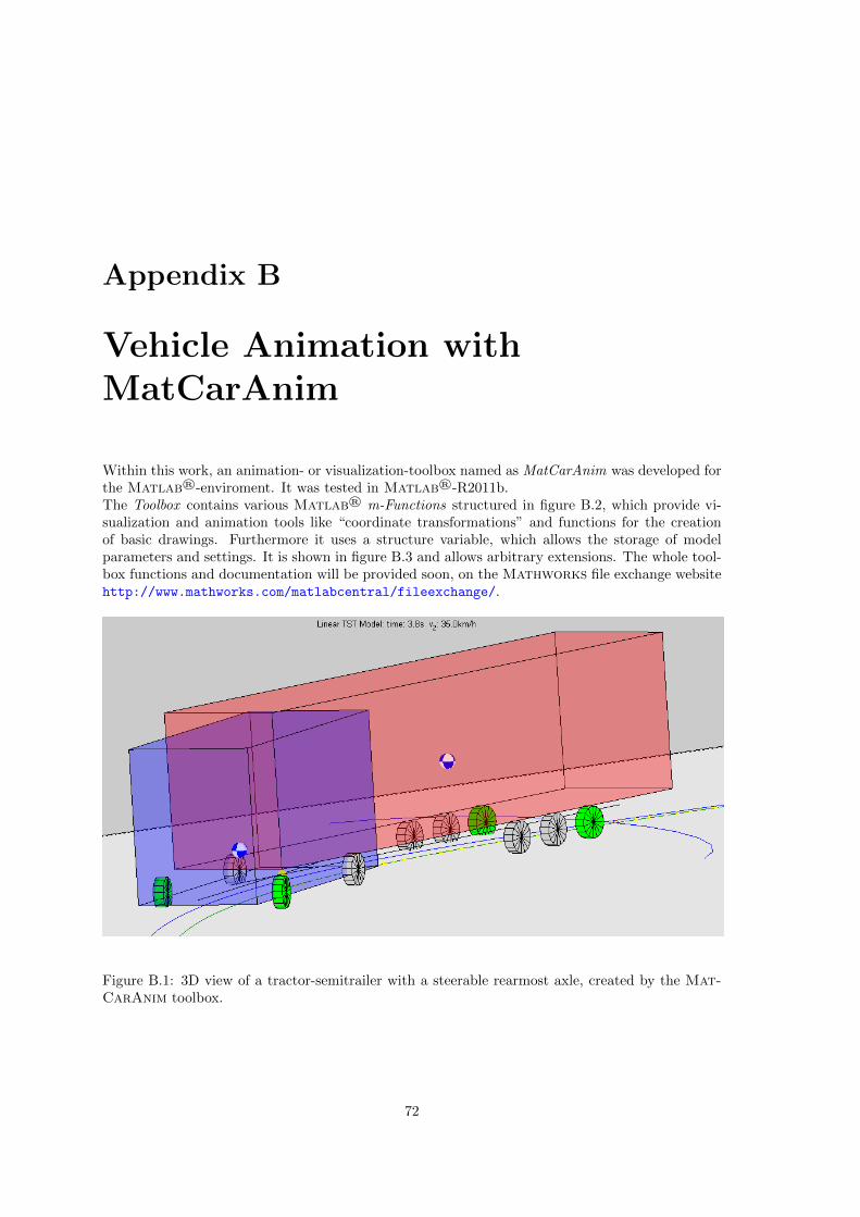
Appendix B
Vehicle Animation withMatCarAnim
Within this work, an animation- or visualization-toolbox named as MatCarAnim was developed forthe Matlab®-enviroment. It was tested in Matlab®-R2011b.The Toolbox contains various Matlab® m-Functions structured in figure B.2, which provide vi-sualization and animation tools like “coordinate transformations” and functions for the creationof basic drawings. Furthermore it uses a structure variable, which allows the storage of modelparameters and settings. It is shown in figure B.3 and allows arbitrary extensions. The whole tool-box functions and documentation will be provided soon, on the Mathworks file exchange websitehttp://www.mathworks.com/matlabcentral/fileexchange/.
Figure B.1: 3D view of a tractor-semitrailer with a steerable rearmost axle, created by the Mat-CarAnim toolbox.
72

Appendix B. Vehicle Animation with MatCarAnim 73
Figure B.2: Structure of the MatCarAnim-software.

74
Figure B.3: Structure of the MatCarAnim-struct.

List of Figures
1.1 Rollover of a real TST in Zhejiang (China) in April 2011. This screen-shots areretouched and extracted from the video of a monitoring camera, published on thewebsite www.youtube.com. . . . . . . . . . . . . . . . . . . . . . . . . . . . . . . . . . 1
1.2 Tractor and semitrailer (TST) with an actively steered rearmost axle. . . . . . . . . 21.3 Tractor with a steered (a) or unsteered (b) semitrailer during a low-speed turning
circle maneuver (german: “BO-Kraftkreis”), required by the European road trafficregulations. . . . . . . . . . . . . . . . . . . . . . . . . . . . . . . . . . . . . . . . . . 2
2.1 Tire axis system and terminology according to SAE-standards [SAE76]. . . . . . . . 52.2 Origin of lateral forces. . . . . . . . . . . . . . . . . . . . . . . . . . . . . . . . . . . . 62.3 Approximation of the lateral force in dependence of the slip angle according to Pace-
jka’s tire model [Pac02] (SAE: Cα < 0). . . . . . . . . . . . . . . . . . . . . . . . . . 72.4 Conception of a single-track-model (Bicycle Model) based on an Ackermann steering. 72.5 Geometric conditions for a single-track-model of a two-axle vehicle for steady state
cornering. . . . . . . . . . . . . . . . . . . . . . . . . . . . . . . . . . . . . . . . . . . 92.6 Single-track-model of a two-axle vehicle at high velocity. . . . . . . . . . . . . . . . . 102.7 Single-track-model of a three-axle truck in a steady-state, very low-speed turn. . . . 122.8 Derivation of the equivalent wheelbase leq of a three-axle truck in a steady-state
low-speed turn. . . . . . . . . . . . . . . . . . . . . . . . . . . . . . . . . . . . . . . . 132.9 Single-track-model of a three-axle truck in steady-state on a very low-speed turn. . . 142.10 Body coordinates of a trailer combination train. . . . . . . . . . . . . . . . . . . . . . 152.11 Steady-state control strategy according to [vdV11]. . . . . . . . . . . . . . . . . . . . 16
3.1 Top view of the Single Track Model of a Tractor and Semitrailer(TST) with a steeredrearmost axle. . . . . . . . . . . . . . . . . . . . . . . . . . . . . . . . . . . . . . . . . 20
3.2 Coordinate transformation of the TST-Single Track Model. . . . . . . . . . . . . . . 233.3 Calculation of the body velocities in order to obtain the body slip angels β1 and β2. 263.4 Top view of the hitch kinematic for the derivation of the coupling condition. . . . . . 273.5 3D view of the hitch kinematic for the derivation of the coupling condition for a
yaw-roll model. . . . . . . . . . . . . . . . . . . . . . . . . . . . . . . . . . . . . . . . 283.6 Roll-extended single track model of the TST with a steered rearmost axle . . . . . . 333.7 Kinematic of the tractor-semitrailer coupling-hitch in the horizontal and vertical
direction. . . . . . . . . . . . . . . . . . . . . . . . . . . . . . . . . . . . . . . . . . . 363.8 Five-DOF tractor-semitrailer model, which includes a rollover consideration. . . . . . 383.9 Screenshot of the multi-body simulation SimPack model. . . . . . . . . . . . . . . . 40
4.1 Feedback control system for the cruise control. . . . . . . . . . . . . . . . . . . . . . 414.2 Feedback control system for the cruise control. . . . . . . . . . . . . . . . . . . . . . 424.3 A hypothetical target-path polygon, defined by path points and created by developed
the functions. . . . . . . . . . . . . . . . . . . . . . . . . . . . . . . . . . . . . . . . . 424.4 Strategy of the virtual drivers controller of the tractor front steer angle δ1. . . . . . . 43
75
76 List of Figures
4.5 Feedback control system for the tractors steering control. . . . . . . . . . . . . . . . 444.6 Considered path point of the virtual driver are limited to a certain range. . . . . . . 44
5.1 Structure of the global process chain for the tractor-semitrailer simulation. . . . . . . 485.2 Simulation structure of the lateral-yaw models for the investigation of the track-tracing. 495.3 Bode diagram of the amplitude frequency response Gψ2δ2
(jω) of the yaw transferfunction at different TST velocities. . . . . . . . . . . . . . . . . . . . . . . . . . . . 50
5.4 Bode diagram of the frequency response Gφ2δ2(jω) of the roll-transfer function at
different TST velocities. . . . . . . . . . . . . . . . . . . . . . . . . . . . . . . . . . . 515.5 Animation of a tractor with an unsteered semitrailer entering a roundabout. The
simulation results were calculated with the “Nonlinear Lateral-Yaw Model”∑
TST
and the animation was created with the Toolbox MatCarAnim. . . . . . . . . . . . 535.6 Position-trajectories of the different models with an unsteered semitrailer and at a
velocity of 20km/h. . . . . . . . . . . . . . . . . . . . . . . . . . . . . . . . . . . . . . 545.7 Trajectories of the nonlinear and linear “Lateral-Yaw-Roll” models with an unsteered
semitrailer and at a velocity of 35km/h. . . . . . . . . . . . . . . . . . . . . . . . . . 55
A.1 Explanation of β1, the body slip angle of the tractor. . . . . . . . . . . . . . . . . . . 63A.2 Single Track Model of Tractor and Semitrailer(TST) with a steered rearmost axle
for the derivation of the linear equations. . . . . . . . . . . . . . . . . . . . . . . . . 64
B.1 3D view of a tractor-semitrailer with a steerable rearmost axle, created by the Mat-CarAnim toolbox. . . . . . . . . . . . . . . . . . . . . . . . . . . . . . . . . . . . . . 72
B.2 Structure of the MatCarAnim-software. . . . . . . . . . . . . . . . . . . . . . . . . 73B.3 Structure of the MatCarAnim-struct. . . . . . . . . . . . . . . . . . . . . . . . . . . 74
Bibliography
[AO98] J. Ackermann and D. Odenthal. Robust steering control for active rollover avoidanceof vehicles with elevated center of gravity. Technical report, DLR, German AerospaceCenter, Institute of Robotics and System Dynamics, 1998.
[AO99] J. Ackermann and D. Odenthal. Damping of vehicle roll dynamics by gain scheduledactive steering. Technical report, DLR, German Aerospace Center, Institute of Roboticsand System Dynamics, Oberpfaffenhofen, D-82230 Wessling, Germany, 1999.
[Boe11] S. Boehl. Lenkstrategie fur einen aktiv gelenkten Sattelauflieger. Semesterthesis, Insti-tute for Dynamic Systems and Control - Swiss Federal Institute of Technology (ETH)Zurich, 2011.
[CC08] C. Cheng and D. Cebon. Improving roll stability of articulated heavy vehicles usingactive semi-trailer steering. Vehicle System Dynamics: International Journal of VehicleMechanics and Mobility, Vol. 46, Supplement:373–388, 2008.
[CP01] B. Chen and H. Peng. Differential-braking-based rollover prevention for sport utilityvehicles with human-in-the-loop evaluations. Vehicle System Dynamics: InternationalJournal of Vehicle Mechanics and Mobility, Vol. 36, No. 4-5:359–389, 2001.
[dB01] D. d. Bruin. Lateral Guidance of All-Wheel Steered Multiple-Articulated Vehicles. Dis-sertation, Technische Universiteit Eindhoven, 2001.
[FMG06] C. Fletcher, C. Manzie, and M. Good. Trailer Steering: An Australian Research Per-spective and Application for By-Wire Control. Technical report, Ninth InternationalSymposium on Heavy Vehicle Weights and Dimensions. June 18-22, Penn State, StateCollege, Pennsylvania, 2006.
[FW07] P. S. Fancher and C. B. Winkler. Directional performance issues in evaluation anddesign of articulated heavy vehicles. Vehicle System Dynamics: International Journalof Vehicle Mechanics and Mobility, Vol. 45, No. 7-8:607–647, 2007.
[Gil92] T. D. Gillespie. Fundamentals of Vehicle dynamics. Society of Automotive Engineers,Warrendale, PA, 1992.
[Hor63] I. M. Horowitz. Synthesis of feedback systems. Academic Press, New York, 1963.
[Jaz09] R. N. Jazar. Vehicle Dynamics: Theory and Application. Springer-Verlag Berlin Heidel-berg, 2009.
[KS88] I. Kageyama and Y. Saito. Stabilization of articulated vehicles by semiactive controlmethod. Vehicle System Dynamics: International Journal of Vehicle Mechanics andMobility, Vol. 17, Supplement 1:199–209, 1988.
[Lun08] J. Lunze. Regelungstechnik 1 - Systemtheoretische Grundlagen, Analyse und Entwurfeinschleifiger Regelungen. Springer-Verlag Berlin Heidelberg, 2008.
77

[OBA99] D. Odenthal, T. Bunte, and J. Ackermann. Nonlinear steering and braking control forvehicle rollover avoidance. Technical report, DLR, German Aerospace Center, Instituteof Robotics and System Dynamics, 1999.
[ORJC10] A. M. C. Odhams, R. L. Roebuck, B. A. Jujnovich, and D. Cebon. Active steering ofa tractor-semi-trailer. Proceedings of the Institution of Mechanical Engineers, Part D:Journal of Automobile Engineering, Vol. 225:847–869, 2010.
[Pac02] H. Pacejka. Tyre and Vehicle Dynamics. Number 0750651415. Elsevier Butterworth-Heinemann, 2002.
[PS10] K. Popp and W. Schiehlen. Ground Vehicle Dynamics. Springer-Verlag Berlin Heidel-berg, 2010.
[SAE76] Vehicle dynamics terminology, SAE J670e, Warrendale, PA, 1976.
[Sam00] D. John M. Sampson. Active Roll Control of Articulated Heavy Vehicles. Dissertation,Cambridge University Engineering Department, 2000.
[SC98] D. J. M. Sampson and D. Cebon. An investigation of roll control system design for artic-ulated heavy vehicles. Technical report, Cambridge University Engineering Department,1998.
[SC03] D. J. M. Sampson and D. Cebon. Achievable roll stability of heavy road vehicles.Proceedings of the Institution of Mechanical Engineers, Part D: Journal of AutomobileEngineering, Vol. 217:217–287, 2003.
[Seg57] L. Segel. Theoretical prediction and experimental substantiation of the response of theautomobile to steering control. Proceedings of the IMechE Automobile Division, pages310–330, 1956-1957.
[Sha05] A. A. Shabana. Dynamics of Multibody Systems. Cambridge University Press, Cam-bridge, 3 edition, 2005.
[SMC99] D. J. M. Sampson, G. McKevitt, and D. Cebon. The development of an active rollcontrol system for heavy vehicles. Technical report, Cambridge University EngineeringDepartment, 1999.
[SW99] R. Schwertassek and O. Wallrapp. Dynamik flexibler Mehrkorpersysteme (in German).Vieweg, Braunschweig, 1999.
[vdV11] B. v. d. Velden. Steering Control of Semi-Trailers – Model-Based Vehicle DynamicsControl for Rollover Prevention. Master’s thesis, Institute for Dynamic Systems andControl - Swiss Federal Institute of Technology (ETH) Zurich, 2011.
[Viv12] M. Vivaldelli. Semi-Trailer Steering Strategies – Model-Based Vehicle Dynamics Con-trollers for Reversing Manoeuvres. Masterthesis, Institute for Dynamic Systems andControl - Swiss Federal Institute of Technology (ETH) Zurich, Swiss Federal Instituteof Technology (ETH) Zurich, 2012.
[Win98] C. B. Winkler. Simplified analysis of the steady-state turning of complex vehicles.Vehicle System Dynamics: International Journal of Vehicle Mechanics and Mobility,Vol. 29:141–180, 1998.
[Zom83] A. Zomotor. Fahrwerktechnik: Fahrverhalten. VOGEL Buchverlag Wuerzburg, 1983.
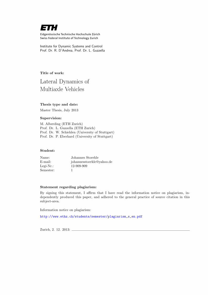
Institute for Dynamic Systems and ControlProf. Dr. R. D’Andrea, Prof. Dr. L. Guzzella
Title of work:
Lateral Dynamics of
Multiaxle Vehicles
Thesis type and date:
Master Thesis, July 2013
Supervision:
M. Alberding (ETH Zurich)Prof. Dr. L. Guzzella (ETH Zurich)Prof. Dr. W. Schiehlen (University of Stuttgart)Prof. Dr. P. Eberhard (University of Stuttgart)
Student:
Name: Johannes StoerkleE-mail: [email protected].: 12-909-909Semester: 1
Statement regarding plagiarism:
By signing this statement, I affirm that I have read the information notice on plagiarism, in-dependently produced this paper, and adhered to the general practice of source citation in thissubject-area.
Information notice on plagiarism:
http://www.ethz.ch/students/semester/plagiarism_s_en.pdf
Zurich, 2. 12. 2013: