Sawtooth SoftwareTECHNICAL PAPER SERIES

The CBC Latent ClassTechnical Paper

(Version 3)

© Copyright 2004, Sawtooth Software, Inc. 530 W. Fir St.

Sequim, WA 98382 (360) 681-2300

www.sawtoothsoftware.com

The CBC Latent Class Technical Paper

Version 3

Copyright 2004, Sawtooth Software, Inc.

Introduction

The Latent Class Segmentation Module is an analytical tool for use with CBC (Choice-Based Conjoint) or CBC/Web studies. It divides respondents into segments having similar preferences based on their choices in CBC questionnaires. It uses latent class analysis for this purpose, which simultaneously estimates part worth utilities for each segment and the probability that each respondent belongs to each segment.

This documentation describes only the capabilities provided by this add-on analytical tool. Readers unfamiliar with CBC should start with the CBC Technical Paper.

Use of latent class analysis as a segmentation method has been examined in many articles in the marketing literature, and it has been found to be effective for that purpose. Thus, it holds promise of solving the problems occurring with aggregate conjoint analysis:

• There is usually sparse information at the individual level for defining segments.

• If there truly are segments with different preferences, an aggregate analysis may give incorrect answers.

Latent class became popular in about the mid-1990s as a tool for analyzing CBC data sets. The model typically provided more insight about the structure of respondent preferences than aggregate logit, and the resulting market simulations were usually more accurate than similarly defined aggregate models. The latent class approach was effective in reducing the negative effects of the IIA assumption in logit analysis. At about the same time, another even more computationally intensive technique called hierarchical Bayes (HB) became available to leading researchers and academics. Latent class provided a discrete model of respondent heterogeneity, whereas HB assumed a continuous model of heterogeneity following a multivariate normal distribution. During the late 1990s, the use of HB for modeling CBC data eclipsed that of latent class in terms of popularity. However, latent class retains a strong following and offers unique benefits. We'll further compare and contrast HB and latent class in the last stage of this documentation.

Running Latent Class Estimation

Latent class has a role analogous to that of CBC’s logit program, but rather than finding average part worth utilities for all respondents together, it detects subgroups with differing preferences and estimates part worths for each segment. The subgroups have the characteristic that the respondents within each group are relatively similar but the preferences are quite different from group to group. You may specify how many groups are to be considered, such as the range of 2 through 6. A report of the analysis is shown on the screen and saved to a log file, and the part worths for subgroups along with each respondent's probabilities of membership in the groups are stored in other files for subsequent analysis or later use by the simulator.

The latent class estimation process works like this:

1. Initially, select random estimates of each group’s utility values.

2. Use each group’s estimated utilities to fit each respondent’s data, and estimate the relative probability of each respondent belonging to each group.

3. Using those probabilities as weights, re-estimate the logit weights for each group. Accumulate the log-likelihood over all groups.

4. Continue repeating steps 2 and 3 until the log-likelihood fails to improve by more than some small amount (the convergence limit). Each iteration consists of a repetition of steps 2 and 3.

Latent class reports the part worth utilities for each subgroup or “segment.” Latent class analysis does not assume that each respondent is wholly “in” one group or another. Rather, each respondent is considered to have some non-zero probability of belonging to each group. If the solution fits the data very well, then those probabilities approach zero or one.

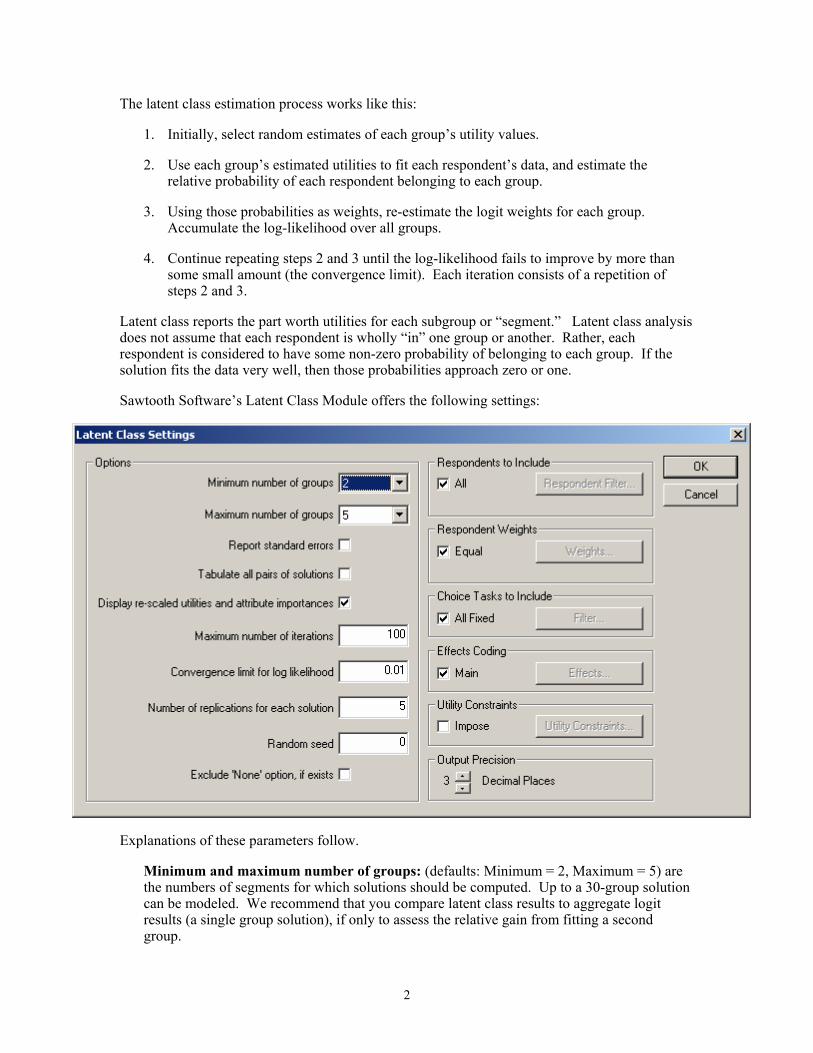
Sawtooth Software’s Latent Class Module offers the following settings:

Explanations of these parameters follow.

Minimum and maximum number of groups: (defaults: Minimum = 2, Maximum = 5) are the numbers of segments for which solutions should be computed. Up to a 30-group solution can be modeled. We recommend that you compare latent class results to aggregate logit results (a single group solution), if only to assess the relative gain from fitting a second group.

2

Report standard errors: Standard errors and t ratios are only reported if this box is checked. The numerical output of Latent Class is much more voluminous than that of Logit, so we have made this information optional.

Tabulate all pairs of solutions refers to tabulations of the respondent group membership for all the solutions with one another. Although each respondent has some probability of belonging to each group, we also classify each respondent into the group to which he or she has highest probability of belonging, and tabulate each solution with those adjacent to it. That is to say, the two-group solution is tabulated against the three-group solution, the three-group solution is tabulated against the four-group solution, etc. If you check this box, then all pairs of solutions are tabulated against each other rather than just those that are adjacent. Note that even if you do not choose to tabulate all pairs of solutions, you can later use the Tables tool in SMRT to cross-tabulate segmentation membership variables you save or import from Latent Class runs.

Display re-scaled utilities and attribute importances determines whether a table is provided within the Latent Class output in which the part worth utilities for each group are re-scaled to be more comparable from group to group (using the normalization method of “zero-centered diffs”). The logit algorithm employed in Latent Class produces utilities close to zero if members of a group are confused or inconsistent in their ratings, and produces larger values if members of a group have consistent patterns of responses. Because groups differ in the scaling of their utilities, it is often difficult to interpret differences from group to group. This table re-scales the part worth utilities for each group to make them comparable: the average range of values for each attribute (the difference between that attribute’s maximum and minimum utilities) is set equal to 100.

Maximum number of iterations (default: 100) determines how long the computation is permitted to go when it has difficulty converging. The default iteration limit is 100, although acceptable convergence may be achieved in many fewer iterations. You may substitute any other iteration limit. If you find that you have specified more iterations than you want to wait for, you can terminate the computation at any time by clicking Stop Operation. The computation will be halted and results for the previous iteration will be saved.

Convergence limit for log-likelihood (default: 0.01) determines how much improvement there must be in the log-likelihood from one iteration to the next for the computation to continue. We arbitrarily use a limit of .01 as a default, but you may substitute a different value. If you find that you have specified too small a convergence limit, you can terminate the computation at any time by clicking Stop Operation. The computation is halted and results for the previous iteration are saved.

Number of replications for each solution (default: 5) lets you conduct automatic replications of each solution from different random starting points. The solution with the highest likelihood for each number of groups is retained as the final solution. If your problem is relatively large, you will probably want to use only one replication in your initial investigation of the data set. However, before accepting a particular solution as optimal, we urge that you replicate that solution from several different random starting points.

Random number seed (default: “0,” meaning random start based on system clock) gives you control of the random number generator that is used to provide the initial random start. The reason for giving you this control is so you can repeat a run later if you want to. Latent class analysis will probably give you a somewhat different solution each time you re-run the analysis with the same data set. The solutions depend on the initial starting values, which are random. If you provide a value here (in the range from 1 to 32000) you will get the same

3

solution each time, but different values will lead to different solutions. If you provide a value of zero, which is the default, then the time of day is used as a seed for the random number generator.

Exclude ‘None’ information, if exists Although you may have included a “None” alternative in your questionnaire, you may not want to include respondents’ propensities to choose that alternative in the information used for segmentation.

Note: For any respondents who choose None for all tasks, there is no information with which to classify them into clusters, and they are automatically classified into the largest cluster.

Respondents to include accesses the same dialog used throughout SMRT for selecting which respondents to include in the analysis.

Respondent weights accesses the same dialog used throughout SMRT for weighting respondents. Weights can be assigned to categories of available segmentation variables (such as demographics, usage questions, etc.). A weighting variable can also be selected, in which case the variable itself contains the weight to be used for each case. Negative numbers are not permitted as respondent weights, and an error message appears if any weight is negative. When weights are used, the maximum and minimum weights are computed and reported in the output, and a message is printed saying that standard errors and t ratios may not be accurate.

Choice tasks to include accesses the same dialog used within SMRT for selecting which choice tasks to include in estimation. By default, all random choice tasks are included. Click this button to select a subset of the random tasks, or to add any available fixed tasks to the estimation.

Effects coding lets users specify whether to include main effects only, or add additional first-order interaction effects. Additionally, this accesses a dialog where linear terms may be specified for attributes rather than using the default part worth model.

Utility constraints accesses a dialog in which you can specify utility constraints (also known as monotonicity constraints). This can be useful for constraining part worths (or signs for linear coefficients) to conform to rational expectations.

Output precision controls the number of decimal places of precision that are used when displaying values to the screen. Please note that the choice here doesn’t affect how SMRT stores the part worths and probabilities of membership, or how it stores runs internally when automatically writing Latent Class runs for use in the market simulator.

Estimating Interaction Effects

Our implementation of Latent Class estimation by default assumes a main effects (additive) model. Most of the information regarding respondent preferences is usually captured with main effects. However, sometimes interaction effects can significantly improve model fit, and CBC analysis under Latent Class permits inclusion of first-order interaction effects (two-way interactions between attributes).

4

For example, consider two attributes (automobile models and colors):

Car Color Convertible Black Sedan Grey Limousine Red Under main effects assumptions, we assume that we can accurately measure preferences for car types independent of the color. However, the color red goes exceptionally well with convertibles and generally not so well with limousines. Therefore, there indeed may be a relatively strong and important interaction effect between car and color. The interaction terms may indicate a decrease in the net utility of a red limousine after accounting for the main effects of limousine and the color red, and an increase in the net utility of a red convertible after accounting for the main effects of convertible and the color red.

CBC is an excellent tool for measuring all potential two-way interactions among attributes. However, many of the interactions we observe in aggregate analysis (such as with aggregate logit), are largely due to unrecognized heterogeneity. It is entirely plausible that a latent class analysis may uncover different groups of respondents: a group that prefers convertibles, a group that prefers sedans, and a group that prefers limousines. And, it may also detect that the group that prefers convertibles also tends to prefer the color red, and the group that prefers limousines also tends to reject red as a color for the automobiles they choose. If this occurs, then the latent class solution used within market simulations will indicate a “revealed” interaction during sensitivity simulations (after accumulating shares across segments), even though an interaction between model and color was never specified in the model. For example, if a black limousine is changed (through sensitivity analysis) to a red color, those respondents principally contributing share to that product would react quite strongly, reducing its share to a greater degree than if either a convertible or a sedan were modified from black to red. To the degree that interactions observed in conjoint data sets are due principally to unrecognized heterogeneity, methods that model heterogeneity, such as latent class, may obtain excellent model fit using just main effects models.

The above example involving automobiles and colors was deliberately extreme, to convey the point. It is possible that in the real world an additional first-order interaction would be required between model and color, because the interaction may indeed occur within each individual’s utility structure, rather than be an interaction observed due to respondent heterogeneity.

In the previous example, we argued in favor of more parsimonious models within latent class, such as main effects only. However, some data sets may indicate the presence of significant interaction terms, even after accounting for heterogeneity, and latent class often provides very good estimation of interaction effects, particularly if you have relatively large sample sizes.

Linear Variables

You can treat quantitative attributes as linear rather than as discrete. For example, suppose you have a price variable with five price levels. The standard approach is to solve for separate part worth utilities for those five discrete levels. With Latent Class, you have the option of fitting a single linear coefficient to the five price levels, which requires estimating only one parameter rather than four (five levels, minus one for effects-coding). This capability may be useful for several reasons:

5

Smoothing noisy data: Often in conjoint analysis we know that levels of an attribute have an a priori order, and we want the resulting utilities to display that order. However, unless the sample is very large, random error may cause some part worth values to display order reversals. For example, we usually want higher prices to have lower utilities. Sometimes we may even be confident of the shape of the curve relating utility to the underlying attribute. If we can assume utility is linearly related to the log of price, then all the information in our data is concentrated on estimating the single parameter which represents the steepness of the utility curve, and we can be assured that the resulting utilities will lie on a smooth curve.

More power to study interactions: The usual way to handle interactions is to estimate separate coefficients for each combination of levels. For example, with 5 brands and 5 price levels, there are a total of 25 combinations, each of which needs to be estimated in some way. Often, the size of the largest interaction dictates the sample size for the study. However, if we could treat price as a linear or log-linear variable, we would only need to estimate five values, the slope of the price curve for each brand. Even more dramatically, if we have two attributes that can be regarded as linear, such as price and, say, speed, then we could handle both main effects and their interaction with a total of only three coefficients.

More parsimonious models: If linear relationships hold for intermediate levels, you can conserve degrees of freedom relative to part worth models.

Of course, to use this capability properly, you must be confident of the shapes of the underlying utility curves. Latent class can be of some help in that regard as well, since you can use trial and error to see whether you achieve better fit with linear values, their logs, or other transformations. We should note that analysts often find that more parsimonious models often improve individual levels of fit (such as hit rates), but often reduce aggregate measures of fit (such as share prediction accuracy). Therefore, the modeling goals influence the decision regarding whether to fit linear terms rather than part worths.

Monotonicity (Utility) Constraints:

Sometimes there are attributes such as speed, quality, or price, where the levels have a natural order of preference. Higher speeds are preferred to lower speeds, higher quality to lower quality, and lower prices to higher prices (all else being equal). Given a good study design, execution, and adequate sample size, part worths (when summarized across groups in latent class) rarely depart from the expected rational order for such attributes. However, some studies reflect reversals in naturally ordered part worths. These reversals are usually due to inadequate sample size and can be explained as due to random error. Even so, reversals can be disconcerting for clients, and in some cases can detract from predictive accuracy. With higher-dimension solutions in latent class, reversals are quite common within groups, though they are typically not present when viewing the summarized results across groups.

Latent class provides an effective manner for “smoothing” reversals (within group) using monotonicity constraints. These constraints often improve individual-level predictions. They also tend to keep higher-dimension solutions “better behaved,” helping control overfitting and leading to more meaningful and interpretable within-group preferences. But, constraints should be used with caution, as it is our experience that they can sometimes slightly reduce share prediction accuracy.

6

We have described the use of constraints for attributes with discrete levels, but not for attributes treated as linear, for which single parameters are estimated. Those attributes may be constrained to have positive or negative signs. For example, with price, it seems reasonable to constrain the sign of the coefficient to be negative so that higher prices correspond to larger negative utilities. With a performance attribute, it might be reasonable to constrain the sign to be positive.

If you employ constraints, a message to that effect appears in the output, and you are warned that standard errors and t values may not be accurate.

How the SMRT Simulator Uses Latent Class Utilities With Latent Class, rather than computing a set of part worths (utilities) for each respondent, the algorithm finds groups of respondents with similar preferences and estimates average part worths within these segments. As when using cluster analysis, the Latent Class analyst specifies how many groups to use in the segmentation. In contrast to cluster analysis, respondents are not assigned to different segments in a discrete (all-or-nothing) manner under Latent Class analysis, but have probabilities of membership in each segment that sum to unity. The sum of the probabilities of membership across respondents for each group defines the total weight (class size) of that segment. One can conduct overall market simulations with Latent Class results by computing shares of preference within each segment and taking the weighted average of these shares across segments. Another way to use Latent Class data is to convert the segment-based results into individual-level estimates. While these estimates are not as accurate at characterizing respondent preferences as ICE or Hierarchical Bayes analysis, they are an appropriate extension of the Latent Class model. When you save a Latent Class run for use in the SMRT simulator, or when you import latent class runs from the Run Manager in SMRT, SMRT converts the group-based Latent Class part worths into individual-level part worths in the following way: For each respondent, a weighted combination of the group part worth vectors is computed, where the weights are each respondent’s probabilities of membership in each group. Converting the Latent Class utilities to individual-level part worths provides added flexibility for market simulations. It lets the analyst apply segmentation variables as filters, banner points or weights without requiring that a new Latent Class solution be computed each time. (You can export the individual-level part worths to an Excel-friendly .csv file from Run Manager, by choosing the latent class run and clicking Export.) However, creating individual-level utilities from a segment-based solution slightly alters the results compared to the method of estimating weighted shares of preference across groups. While the overall shares of preference for the market are nearly identical, the within-class results reported in the Market Simulator output are slightly less differentiated between segments (pulled toward the overall market mean). That is because for the purpose of banner points and filters, the Market Simulator assigns respondents fully into the latent class for which he/she has the greatest probability of membership. For example, consider a respondent whose preferences are characterized as 80% like group 1 and 20% like group 2. His contribution to the mean values reported in the group 1 column (banner point) includes some group 2 tendencies. The differences between the within-class means reported by Latent Class and the Market Simulator are not very strong, since respondents’ probabilities of membership in classes usually tend toward zero or one. The smoothing that occurs when reporting the by-segment results in the Market Simulator will probably not substantially change your interpretation of the results. If the

7

differences concern you, you can always refer to the original Latent Class output, and run simulations based on the group-level part worths, weighted by the segment sizes. You can do this using your own tools, or by modifying the .LCU file to conform to the .HBU layout, importing the .HBU through Run Manager and applying segment-based weights during simulations.

A Numeric Example

In this section we present and describe the latent class analysis of a sample data set named “lsample,” which is provided with the Latent Class Module installation. This example uses an artificial data set constructed as follows: First, part worth utility values were chosen for three hypothetical groups on three attributes:

Hypothetical Utilities for Three Segments Segment 1 Segment 2 Segment 3 (N = 80) (N = 160) (N = 240)

Brand 1 2.0 -1.0 -1.0 Brand 2 -1.0 2.0 -1.0 Brand 3 -1.0 -1.0 2.0

Pack 1 -1.0 -1.0 -1.0 Pack 2 -1.0 -1.0 2.0 Pack 3 2.0 2.0 -1.0

Price - - 2.0 2.0 2.0 Price - 1.0 1.0 1.0 Avg Price 0.0 0.0 0.0 Price + -1.0 -1.0 -1.0 Price ++ -2.0 -2.0 -2.0

One hypothetical group likes each brand best. Pack 3 is preferred by two groups and Pack 1 is preferred by no group. All agree on the desirability of paying lower prices.

From these utilities, artificial data for 480 respondents were constructed. We drew 80 simulated respondents from the first segment, 160 from the second, and 240 from the third. A CBC questionnaire was created for each individual, containing 20 tasks, each presenting three alternatives plus a “None” option. Answers for each question were simulated by first summing the respondent’s utilities for each alternative, adding a random component to each sum, and then selecting the highest of the resulting values. The random components were distributed double-exponentially with variance of unity.

We have chosen an example based on simulated data rather than data from real respondents because with simulated data we know what the “right answer” is: that there are really three segments of sizes 80, 160, and 240, and the pattern of utilities for each segment.

One of the problems in interpreting logit-based utilities is that logit analysis stretches or shrinks its parameter estimates according to the goodness of its fit. If the data for a group are fit very well, its utilities tend to be far from zero. If the data for a group are fit poorly, the utilities will be closer to zero. Because some groups may be fit better than others, it can be confusing to compare results for different groups. To facilitate such comparisons, we provide the option of re-scaling each group’s estimated utilities so the average range within an attribute is 100. To provide a “target” against which to later compare the estimated utilities, we scale the above hypothetical utilities in the same way:

8

Hypothetical Utilities, Re-scaled for Comparability

Segment 1 Segment 2 Segment 3 (N = 80) (N = 160) (N = 240)

Brand 1 60 -30 -30 Brand 2 -30 60 -30 Brand 3 -30 -30 60

Pack 1 -30 -30 -30 Pack 2 -30 -30 60 Pack 3 60 60 -30

Price - - 60 60 60 Price - 30 30 30 Avg. Price 0 0 0 Price + -30 -30 -30 Price ++ -60 -60 -60

In conjoint analysis we sometimes summarize the relative importance of an attribute by expressing its range in utility to the sum of the ranges for all the attributes. We do that here, finding that for every segment, Brand and Pack each has importances of 30%, and Price has an importance of 40%.

Attribute Importances Segment 1 Segment 2 Segment 3

Brand 30 30 30 Pack 30 30 30 Price 40 40 40

A Sample Computation:

Latent Class Analysis for 3 Groups Iteration Log-likelihood Gain Segment Size 0 -13308.43 1 -8087.70 5220.73 50.0 48.7 1.3 2 -5225.99 2861.71 50.0 33.5 16.5 3 -3896.64 1329.35 50.0 33.3 16.7 4 -3736.11 160.53 50.0 33.3 16.7 5 -3726.19 9.92 50.0 33.3 16.7 6 -3726.02 0.17 50.0 33.3 16.7 7 -3726.02 0.00 50.0 33.3 16.7 Percent Certainty = 72.00 Consistent Akaike Info Criterion = 7746.96 Chi Square = 19164.81 Relative Chi Square = 660.86

We start with estimates of respondent utilities that are just random numbers, and improve them, step by step, until the final solution fits the data acceptably well. The latent class algorithm uses a maximum likelihood criterion. Given its estimates of segment utilities and group sizes at each stage, the algorithm computes the probability that each respondent should have selected the alternative he or she did. The log likelihood is obtained by summing the logs of those probabilities, over all respondents and questions.

In this questionnaire there are 480 respondents, each of whom answered 20 questions, each of which had 3 product alternatives and a “none” option. Under the “null” condition of utilities of zero, any answer would have a probability of .25. The log of .25 is -1.38629. Multiplying that

9

by the number of respondents (480) and the number of questions (20) gives the “null” log likelihood listed at iteration 0.

If we were able to predict every respondent’s answers perfectly, all the probabilities would be unity, and their logs would be zero. Therefore, the most favorable possible log likelihood is zero. This computational procedure starts with a random solution which is modified iteratively, with each successive solution having a higher likelihood. For each iteration we print the resulting likelihood as well as the gain as compared to the previous iteration. The gains are large in initial iterations, and then become successively smaller in later iterations.

If you accept the built-in default values, the process is halted when a maximum of 100 iterations is reached, or when the gain is less than 0.01. Those are both arbitrary values, and if we had chosen a less rigorous limit of, say, 1.0, the process would have been complete after 6 iterations.

To the right of the “gain” column are three columns of values that add to approximately 100. These are the estimates made during each iteration of the relative sizes of the segments. Recall that we constructed our synthetic data to contain three groups of size 80, 160, and 240 respondents. The segmentation algorithm has reproduced those relative sizes accurately (although in a different order) and, indeed, had done so by the third iteration. Below the iteration history is a line of statistics that characterize the goodness of fit of the solution to the data.

“Percent certainty” indicates how much better the solution is than the null solution, when compared to an “ideal” solution. It is equal to the difference between the final log likelihood and the null log likelihood, divided by the negative of the null log likelihood, in this case approximately (-3,726 + 13,308) / 13,308, or 72.00 This measure was first suggested by Hauser (1978), and was used in an application similar to ours by Ogawa (1987). Although “Percent certainty” is useful for providing an idea of the extent to which a solution fits the data, it is not very useful for deciding how many segments to accept because it generally increases as more segments are included.

“Consistent Akaike Information Criterion,” (CAIC) is among the most widely used measures for deciding how many segments to accept. CAIC was proposed by Bozdogan (1987), and an application similar to ours is described in Ramaswamy et al. (1993). Like all measures we report here, CAIC is closely related to the log likelihood. Our implementation of CAIC is given by the formula:

CAIC = -2 Log Likelihood + (nk + k - 1) x (ln N +1)

where k is the number of groups, n is the number of independent parameters estimated per group, and N is the total number of choice tasks in the data set.

Unlike our other measures, smaller values of CAIC are preferred. CAIC is decreased by larger log likelihoods, and is increased by larger sample sizes and larger numbers of parameters being estimated. CAIC is not very useful for assessing the absolute level of fit of a particular solution, but it is sometimes useful when looking across alternative solutions with different numbers of groups.

Chi Square is twice the log likelihood for the solution, minus twice the log likelihood for the null solution. It can be used to test whether a solution fits significantly better than the null solution, although that is almost always true. Chi Square is not very useful for choosing the number of segments because it tends to increase as the number of solutions increases.

10

“Relative Chi Square” is just Chi Square divided by the number of parameters estimated (nk + k - 1). We know of no theoretical basis for this statistic, but Monte Carlo analyses of many data sets has led us to believe that it may be useful for choosing the number of segments. Bigger is better.

Following the measures of fit, estimated utilities for each group are printed. These are “raw” utilities, which may have been stretched or shrunk by different amounts for each group. Although the three segments are of the correct relative sizes, they are not shown in the same order as for the table of “true” utilities above.

Utilities

Segment Size 50.0% 33.3% 16.7% Part Worth Utilities Brand 1 -1.36 -1.99 4.98 Brand 2 -1.40 4.74 -4.36 Brand 3 2.76 -2.75 -0.62 Pack A -1.93 -2.97 -2.50 Pack B 2.95 -1.68 -1.84 Pack C -1.02 4.65 4.34 Price 1 2.55 4.58 5.83 Price 2 2.14 3.92 1.36 Price 3 -0.60 -1.32 1.36 Price 4 -1.99 -3.59 -4.28 Price 5 -2.10 -3.59 -4.28 NONE 0.25 0.68 0.85

Notice that the values for the left-hand column are scaled somewhat smaller than for the other two columns. Those differences make it harder to compare values in adjacent columns, a difficulty which is removed in the table below, in which each column has been re-scaled to “zero-centered diffs” so that its average range within attributes is 100.

Utilities Re-scaled For Comparability

Brand 1 -29.86 -25.69 56.83 Brand 2 -30.63 61.10 -49.73 Brand 3 60.49 -35.41 -7.10 Pack A -42.29 -38.32 -28.52 Pack B 64.60 -21.60 -21.03 Pack C -22.31 59.93 49.55 Price 1 56.02 59.01 66.54 Price 2 46.84 50.47 15.56 Price 3 -13.15 -17.01 15.56 Price 4 -43.75 -46.24 -48.83 Price 5 -45.96 -46.24 -48.83 NONE 5.46 8.76 9.68

The true values have not been recovered perfectly, due to the random error introduced when constructing our artificial data. However, the patterns of high and low values are nearly correct, certainly close enough to characterize each group’s preferences.

The re-scaled utilities immediately above are an option that you may request in the output. If you do, you will also get a table of attribute importances, like the following:

Attribute Importances

Brand 30.37 32.17 35.52 Pack 35.63 32.75 26.02

11

Price 33.99 35.08 38.46

We have not very accurately recovered the true importances of 30% for Brand and Pack and 40% for price for each group, but we are dealing with small sample sizes and fairly noisy data.

One indication that the solution fits the data well is that the average respondent is assigned to a group with probability 1.00. This is much higher than you will see with real data, and is only possible because we started with an artificial data set in which each individual was clearly in one group or another. Finally, if we examine which group each individual was assigned to, the recovery is perfect. We constructed a data set in which the first 80 respondents were from one group, the next 160 from another, and the last 240 from the third. All are classified properly by this solution.

Results were saved for 480 respondents Average maximum membership probability = 1.00 Some parameters were constrained Significance tests and standard errors may not be accurate We are also given a notice that since some parameters were constrained (prices) the optional significance tests and standard errors may not be accurate.

Choosing the Number of Segments:

Next we examine what happens when comparing solutions with different numbers of clusters. We re-ran this computation five times, each time estimating solutions for from 2 to 5 clusters from different starting points (and for comparison, we ran a constrained solution using a 1-group run using v2 of the Latent Class software). For each number of clusters we retained only the solution with highest Chi Square, and those solutions are summarized below:

PctCert CAIC Chi Square RelChiSq 1 Group 26.1 19771.1 6937.2 770.81 2 Groups 57.8 11430.1 15380.0 809.47 3 Groups 72.1 7713.4 19198.4 662.01 4 Groups 73.3 7502.3 19511.2 500.29 5 Groups 75.3 7061.3 20053.8 409.26

Notice that the PctCert statistic and Chi Square both increase as we increase the number of groups, but don’t increase much after the 3-group solution. This follows expectations, since in theory larger numbers of groups should produce higher values. Also note that using a different starting point, we got a slightly higher fit than for the previous run we reported for the 3-group solution.

CAIC has a minimum for five groups, indicating that it did not work at detecting the correct number of groups. Perhaps more significant is the fact that CAIC decreases dramatically until 3 groups, and then becomes nearly flat for larger numbers of groups. Such an inflection point is probably a better indicator of the right number of groups than its absolute magnitude. Relative Chi Square is maximized for two groups, a disappointment.

We have found that when analyzing real data from human respondents, these statistics are likely to repeat such a pattern, not providing obvious information about the best choice of number of groups. It seems that rather than choosing the solution which provides the highest absolute level of any statistic, it is more useful to look at differences. For example, for Chi Square and Pct Cert we find large increases going from one group to two, and large differences again going from two

12

groups to three. However, beyond that the differences are minimal, suggesting that three might be the right number of groups. Likewise, CAIC drops sharply as we go from one to two and from two to three groups, but then stays fairly constant for solutions with more groups.

When choosing among solutions, one also has access to other information, such as their patterns of utilities and estimated group sizes. Here are the relative group sizes estimated for the five solutions above:

2 Groups 0.500 0.500 3 Groups 0.167 0.333 0.500 4 Groups 0.167 0.333 0.035 0.465 5 Groups 0.154 0.035 0.167 0.465 0.179

Both the four-group and five-group solutions contain tiny groups, emphasized in bold, so they would probably be disqualified on that basis.

You will probably pay close attention to the estimated utilities provided by each solution. Also, each individual can be classified into the group for which he or she has highest probability, and solutions can be further investigated by tabulating them with one another as well as with other variables. You are automatically provided with tabulations of solutions with one another. For example, here is the way respondents were classified by adjacent two-group and three-group solutions in one of the runs.

Tabulation of 2 Group vs. 3 Group Solutions

1 2 3 Total

1 0 0 240 240 2 80 160 0 240

Total 80 160 240 | 480

Every solution that you consider interpreting should be tested by rerunning from several different starting points, and seeing how similar those solutions are to one another.

If the goal of the latent class analysis is managerial relevancy of the segmentation solution, probably the most important aspects to consider when choosing a solution for segmentation purposes are its interpretability and stability (reproducibility). One should repeat the analysis from different starting points (or by randomly splitting the sample into two halves and running the analysis separately on each group) to observe whether similar segments and segment sizes emerge. But if the primary goal for using Latent Class is to create an accurate share simulator, then the accuracy of share predictions should take precedence over segment interpretability and stability. It is sometimes the case that a latent class solution with a larger number of groups can perform better in terms of accuracy than a lower-dimension run that may have clearer interpretability. And, share prediction accuracy may occur with solutions that have more groups than the previously discussed statistical criteria might justify. Some Latent Class users save one run for the purposes of simulations, but use another run for interpretable segment classification. The interpretable segment classification may be used as a banner point (e.g. filter), and the more accurate latent class utility run may be used for estimating shares and reporting utilities.

13

Practical Problems in Latent Class Analysis:

We have used a sample data set for which the latent class algorithm is comparatively well behaved. However, we want to avoid giving the impression that latent class analysis is simple, or that its interpretation is straightforward. It does present several difficulties. To illustrate some of these, we reran the sample problem five more times.

Timing: For very large problems, Latent Class can take many minutes (if not multiple hours) to run. Latent Class v3 is significantly faster than earlier versions, and computer speeds continue to increase, so speed is much less an issue than just a few years ago. Generally, Latent Class is slower than logit, but faster than hierarchical Bayes (HB).

Optimality: In the example described above, we used the default convergence limit of 0.01. For the two-group solutions, Latent Class got the same solution every time in the sense that it always classified respondents the same way.

For the three-group solutions, Latent Class got the solution reported above three times. However the other three times it got a different solution, similar to the 2-group solution but with a tiny splinter group. The correct solution had dramatically higher likelihood than the incorrect one, so there is no question about which is superior.

One of the most severe problems with latent class analysis is vulnerability to local maxima. The only way to avoid this problem is to compute several solutions from different starting points. Latent Class will choose different starting points for each run automatically unless you specify otherwise.

For four and five groups, different solutions were found every time--the data do not naturally support stable four- or five-group solutions. As it was, they classified respondents similarly about 80% of the time. However, nearly all of them would be rejected for containing tiny groups.

You may find that the iterative process converges rapidly. However, depending on your data or an unfortunate random starting point, you may also encounter either of the following:

Convergence may be slow. You may reach the limit on number of iterations before your successive gains are smaller than the convergence limit. If that happens, you receive a warning message both on screen and in your printed output. In that case, it is possible that no clear segmentation involving that number of groups exists for those data, and further exploration with that number of groups may not be worthwhile. However, we suggest that you try again, with different starting points and a higher iteration limit.

The system may become “ill-conditioned.” This means that there is not enough information to estimate all the parameters independently of one another. This message is a symptom of too many segments, too many parameters, or too little data. (It may also indicate an unacceptable pattern of prohibitions in your questionnaire.) This message is often an indication that at least one group has become tiny. If you receive this message, try again from a different starting point. If you receive it repeatedly, but only for large numbers of segments, you may have to be satisfied with fewer segments. If you receive it with a small number of segments, it may be necessary to alter your effects file so as to estimate fewer parameters.

These difficulties may tempt you to abandon latent class analysis. Although we think it is important to describe the difficulties presented by Latent Class, we think it is the best way

14

currently available to find market segments with CBC-generated choice data. In the next section we describe how we came to that point of view.

Why Latent Class Analysis?

The disadvantage of analyzing choices rather than rankings or ratings is that choices contain less information, so choice studies in the past were most often analyzed by aggregate methods. This lead to two problems:

• Since no utilities were available for individual respondents, it was hard to use the choice data to develop market segments based on choice behavior.

• In an aggregate analysis, the logit model assumes that the only variability among respondents is random, indistinguishable from response error. If there really are distinct segments, consisting of groups of respondents who are relatively similar to one another but who differ from group-to-group, then the aggregate model will not be appropriate.

A lot of attention has been given to these problems and many relevant articles have appeared in the literature. Three kinds of solutions have been proposed:

1. Latent class and similar methods attempt to find groups of respondents who share similar preferences and utilities. Latent class methods permit each respondent to have some positive probability of belonging to each class, and solve simultaneously for the utilities for each class and for each respondent’s probability of belonging to each. Other methods assume each respondent belongs entirely to one cluster or another, and attempt simultaneously to allocate respondents to clusters and solve for utilities for each cluster.

Moore, Gray-Lee, and Louviere (1996) explored several methods for segmenting respondents, based on both choice and conjoint data. For choice data they found that a “latent segment” approach produced better results than aggregate analysis or clustering on choice data directly. Their approach attempted to find a partitioning of respondents that maximized a likelihood criterion, with every respondent allocated to one segment.

Vriens, Wedel, and Wilms (1996) compared nine methods of segmenting respondents, using conjoint data (rather than choices) in a Monte Carlo study. They found latent class procedures to perform best at recovering known data structure.

DeSarbo, Ramaswamy, and Cohen (1995) demonstrated the use of latent class analysis with choice data, using a data set for 600 respondents. They found that a four-segment latent class solution fit the data much better than the aggregate solution, and also much better than a four segment solution produced with cluster analysis.

2. Highly-efficient customized experimental designs permitted Zwerina and Huber (1995) to compute utilities at the individual level. Their data set was a small one, but their results suggest that it may be possible to obtain individual utilities from choice data. A related possibility would be an approach like that of ACA, in which choices are combined with information from self-explicated preferences.

In a Sawtooth Software Conference Proceedings paper (2003), Johnson investigated a new method for creating customized choice designs on-the-fly during a computerized interview. This approach used aspects of ACA (self-explicated exercise followed by

15

customized experimental designs) to improve the efficiency and accuracy of choice estimation at the individual level.

3. Hierarchical Bayes methods were studied by Lenk, DeSarbo, Green, and Young (1996) with full profile conjoint data, although it seems likely that they would have achieved similar results for choices. They found that Hierarchical Bayes analysis was able to estimate reasonable individual utilities, even when using responses to fewer profiles than the number of parameters estimated for each respondent. Individual Hierarchical Bayes utilities did a better job of predicting hit rates for holdout concepts than conventional OLS estimates, even when based on only half as many profiles.

Since the mid-1990s, HB has received ever-increasing attention in the literature and at leading methodological conferences, and has proven very useful and popular. HB analysis (as offered by our CBC/HB software) can provide robust individual-level estimates from relatively little data per individual.

Clusterwise Logit vs. Latent Class

By combining elements of cluster and logit analysis, it is possible to find segments of respondents in a simple and straightforward way. Our initial investigation into this subject used an approach similar to that of Moore et al.(1996). We constructed a segmentation/estimation module by combining CBC’s Logit module with elements of our K-Means cluster analysis product, CCA. We called this method “Klogit,” which went like this:

1. Set the number of clusters, and choose an initial solution for each cluster consisting of random numbers in the interval -0.1 to 0.1.

2. Use each group’s values to fit each respondent’s data, using a logit model. (Of course, the initial solutions will not fit anybody at all well.) Reallocate each respondent to the group whose coefficients provide the best fit.

3. Estimate a logit solution for the respondents in each group.

4. Repeat steps 2 and 3 until no respondents change groups.

We used Monte Carlo methods to investigating Klogit’s ability to recover known cluster structures. It did quite well, and we would base our CBC segmentation module on Klogit if we had not also had experience with latent class estimation. However, because of the favorable reports on latent class methods in the references above, we further extended CBC’s Logit algorithm to perform latent class analysis. Our algorithm, Latent Class, is more complicated than Klogit, but not very much so, and goes like this:

1. As with Klogit, set the number of clusters, and choose a random initial solution for each cluster with values in the interval -.1 to .1.

2. As with Klogit, use each group’s logit coefficients to fit each respondent’s data, and estimate the likelihood of each respondent’s belonging to each class.

3. Estimate a weighted logit solution for each class. Each solution uses data for all respondents, with each respondent weighted by his or her estimated probability of belonging to that class.

16

4. Underlying this method is a model which expresses the likelihood of the data, given estimates of group coefficients and groups sizes. Compute the likelihood of the data, given those estimates.

5. Repeat steps 2 through 4 until the improvement in likelihood is sufficiently small.

Our implementation of the latent class algorithm is based on the description by DeSarbo, Ramaswamy, and Cohen (1995), who provide the likelihood equation that we use as well as some further details of the estimation procedure.

We do not produce the likelihood equation here because of typographic limitations. However, log-likelihood is computed as follows:

1. For each individual, compute the probability of each choice that was made, assuming the individual belonged to the first group. Multiply together those probabilities for all tasks to get a likelihood of that individual’s data, assuming membership in the first group. Also make a similar computation assuming membership in each other group.

2. Weight the individual’s likelihood for each group (as just described) by the current estimate of that group’s size. (The group size estimates sum to unity.) Sum the products over groups, to get a total (weighted) likelihood for that individual.

3. Cumulate the logs of those likelihoods over individuals.

Individual probabilities of belonging to each group are obtained by percentaging the weighted likelihoods obtained by steps 1 and 2. Relative group size estimates are obtained by averaging those values over respondents.

We have compared Latent Class and Klogit in many Monte Carlo studies, with these results:

• Klogit is much faster than Latent Class, by an average factor of about 3.

• For Monte Carlo data with random response error but no heterogeneity within segment, Klogit and Latent Class do about equally well. With moderate response error they both obtain the correct solution almost every time, and they do quite well even with very large response error.

• However, when the data contain within-cluster heterogeneity, Latent Class pulls ahead. Latent Class is more reproducible when repeated solutions are computed from different starts, recovers known solutions better, and also produces groups more nearly of the right size.

One of our principles at Sawtooth Software is to try to produce tools that work every time. That leads us to select the more robust and stable Latent Class method, despite the fact that Klogit is conceptually simpler and much faster.

17

HB vs. Latent Class

As mentioned in the introduction to this documentation, hierarchical Bayes (HB) is used more often today to analyze CBC data. Still, Latent Class offers unique benefits, and it has a strong following.

Latent class may be particularly beneficial in the following circumstances:

• Often one of the goals of a CBC project is to learn more about the natural market segments that might exist in a population. A marketing manager might benefit from knowing about the different preferences across segments, especially if these segments have targetable differences beyond just preferences. Latent class provides an effective way to discover segments, and the statistics it provides for determining an appropriate number of segments are argued to be superior than those for the usual alternative of cluster analysis. Although it is possible to run cluster analysis on the results of HB analysis, we expect that analysts can achieve slightly better results if using the one-step latent class procedure.

• If respondents are really segmented into quite compact and differentiated groups in terms of preference, the discrete assumption of heterogeneity used in latent class can more accurately model individuals than HB.

HB has the following strengths:

• If respondents seem to be distributed in a more continuous rather than discrete fashion in terms of their multidimensional preferences, then HB can more accurately reflect individuals’ preferences. We would argue that most data sets usually involve a relatively continuous distribution of heterogeneity, which is more in harmony with HB's assumptions. HB is also quite robust even when there are violations of the underlying assumptions. It is not surprising, therefore, that hit rates (individual-level prediction accuracy of holdout tasks) from HB almost always exceed those for Latent Class for typical CBC data sets.

• Market simulations using the individual-level part worths resulting from HB estimation are usually a bit more effective than Latent Class in reducing IIA problems.

We know of at least two recent studies in which individual-level estimates from HB did not improve predictive fit over aggregate logit or latent class solutions. The first study (Pinnell, Fridley 2001) demonstrated better hit rates of holdout tasks for aggregate logit than HB for some commercial partial-profile CBC data sets (HB was also superior for some partial-profile CBC data sets). In another recent study (Andrews, Ainslie, Currim 2002), better household-level prediction was achieved with latent class and logit than HB for simulated scanner choice data when the number of simulated purchases was only three per household and seven parameters were fit (with more data available at the household level, HB performed as well as latent class, with better internal fit). In both cases where HB seemed to perform worse than aggregate methods, the data were exceptionally sparse at the individual level and HB was subject to overfitting. We speculate that the narrow margin of victory for aggregate methods over HB in both cases may have been due to sub-optimal specification of the priors (prior covariance, and degrees of freedom for the prior covariance matrix). We have re-analyzed two of the data sets reported by Pinnell and Fridley, and after adjusting HB priors (assuming lower heterogeneity and a greater weight for the prior) found that HB’s hit rates slightly exceeded that of aggregate logit.

18

We haven’t examined the simulated household data of Andrews, Ainslie and Currim, so we can only speculate that modified HB priors may have affected their conclusions.

We'll conclude with two more observations:

• If the principal goal of the research is to develop an accurate group-level market simulator, then latent class has been shown to offer simulation accuracy that approaches (and has been reported by some authors to occasionally exceed) the accuracy of HB.

• Some researchers have learned to leverage the strengths of both techniques within their CBC analysis. They use latent class to detect segments, and use the segment membership information as “banner points” (filters) applied to simulations using underlying HB utility runs.

19

20

References Andrews, R. L., Ainslie, A., and Currim, I. S., “An Empirical Comparison of Logit Choice Models with Discrete Versus Continuous Representations of Heterogeneity,” Journal of Marketing Research, November 2002, p 479-487.

Bozdogan, H. (1987), “Model Selection and Akaike’s Information Criterion (AIC): The General Theory and its Analytical Extensions,” Psychometrika, 52, 345-370.

DeSarbo, W. S., V. Ramaswamy, and S. H. Cohen (1995), “Market Segmentation with Choice-Based Conjoint Analysis,” Marketing Letters, 6, 137-148.

Hauser, J. R. (1978), “Testing and Accuracy, Usefulness, and Significance of Probabilistic Choice Models: An Information-Theoretic Approach,” Operations Research, 26, (May-June), 406-421.

Johnson, Richard M. (2003), “Adaptive Choice-Based Conjoint,” Sawtooth Software Conference Proceedings (forthcoming).

Lenk, P. J., W. S. DeSarbo, P. E. Green, and M. R. Young (1996), “Hierarchical Bayes Conjoint Analysis: Recovery of Partworth Heterogeneity from Reduced Experimental Designs,” Marketing Science, 15 (2) 173-191.

Moore, W. L., J. Gray-Lee and J. Louviere (1996), “A Cross-Validity Comparison of Conjoint Analysis and Choice Models at Different Levels of Aggregation,” Working Paper, University of Utah, November.

Ogawa, K. (1987), “An Approach to Simultaneous Estimation and Segmentation in Conjoint Analysis,” Management Science, 6, (Winter), 66-81.

Pinnell, Jon and Fridley, Lisa (2001), “The Effects of Disaggregation with Partial Profile Choice Experiments,” Sawtooth Software Conference Proceedings, Sequim WA, 151-165.

Ramaswamy, V. , W. S. DeSarbo, D. J. Reibstein, and W. T. Robinson. (1993), “An Empirical Pooling Approach for Estimating Marketing Mix Elasticities with PIMS Data.” Marketing Science, 12 (Winter), 103-124.

Vriens, M., M. Wedel and T. Wilms (1996), “Metric Conjoint Segmentation Methods: A Monte Carlo Comparison,” Journal of Marketing Research, 33,(February) 73-85.

Zwerina, K. and J. Huber (1996) “Deriving Individual Preference Structures from Practical Choice Experiments,” Working Paper, Duke University, August.