Latent Class Analysis - Jonathan Templin's Website theory ... Much less often, latent class analysis is included in the group. ... a binary-response item,X

®

September 18, 2008 Slide 1 of 54

Latent Class Analysis

ERSH 9800: Diagnostic Modeling

Overview● Talk Outline● Initial Distinctions

Latent ClassAnalysis

LCA Example

Assessing Model Fit

LCA Wrap Up

®


Talk Outline

● Latent Class Analysis (LCA).

✦ Underlying theory (general contexts).

✦ Example analysis (and how to get estimates).

✦ Interpretation of model parameters.

✦ Investigating model fit.



LCA Example

Assessing Model Fit

LCA Wrap Up

®


Clusters Versus Classes

● When a researcher mentions they are going to be usingcluster analysis, they are most likely referring to one of thefollowing:

✦ K-means clustering.

✦ Hierarchical clustering using distance methods.

✦ Discriminant analysis.

✦ Taxometrics.

● Much less often, latent class analysis is included in thegroup.

✦ Although it too is useful for detecting clusters ofobservations.

● For today’s talk, we will consider clusters to be synonymouswith classes.



LCA Example

Assessing Model Fit

LCA Wrap Up

®


LCA Versus Other Methods

● Although I am using the terms classes and clusterssynonymously, the general approach of LCA differs from thatof the other methods previously discussed.

● LCA is a model-based method for clustering (orclassification).

✦ LCA fits a statistical model to the data in an attempt todetermine classes.

● The other methods listed on the previous slide do notexplicitly state a statistical model.

● By being model based, we are making very explicitassumptions about our data.

✦ Assumptions that can be tested.


Latent Class Analysis

Overview

Latent ClassAnalysis● Input Variables● Analysis Process● Estimation● Assumptions● Bernoulli● Independence● Finite Mixture

Models● LCA as a FMM● Local

Independence● Estimation

Process● Software for LCA

LCA Example

Assessing Model Fit

LCA Wrap Up

®


LCA Introduction

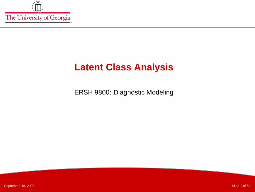
● Latent class models are commonly attributed to Lazarsfeldand Henry (1968).

● The final number of classes is not usually predeterminedprior to analysis with LCA.

✦ The number of classes is determined through comparisonof posterior fit statistics.

✦ The characteristics of each class is also determinedfollowing the analysis.

✦ Similar to K-means and hierarchical clustering techniquesin this respect.

Overview





LCA Example

Assessing Model Fit

LCA Wrap Up

®


Variable Types Used in LCA

● As it was originally conceived, LCA is an analysis that uses:

✦ A set of binary-outcome variables - values coded as zeroor one. Examples include:

■ Test items - scored correct or incorrect.

■ True/false questions.

■ Gender.

■ Anything else that has two possible outcomes.

Overview





LCA Example

Assessing Model Fit

LCA Wrap Up

®


LCA Process

● For a fixed number of classes, LCA attempts to:

✦ Estimate the probability that each variable is equal to onefor each class (class specific item difficulty).

✦ Estimate the probability that each observation falls intoeach class.

■ For each observation, the sum of these probabilitiesacross classes equals one.

■ This is different from K-means where an observation is amember of a class with certainty.

✦ Across all observations, estimate the probability that anyobservation falls into a class.

Overview





LCA Example

Assessing Model Fit

LCA Wrap Up

®


LCA Estimation

● Estimation of LCA model parameters can be morecomplicated than other clustering methods:

✦ In hierarchical clustering, a search process is used withnew distance matrices being created for each step.

✦ K-means uses more of a brute-force approach - tryingmultiple random starting points then shifting casesbetween the different clusters until each is no longershifted.

✦ Both methods relied on distance metrics to find clusteringsolutions.

● LCA estimation uses distributional assumptions to findclasses.

● The distributional assumptions provide the measure of"distance" in LCA.

Overview





LCA Example

Assessing Model Fit

LCA Wrap Up

®


LCA Distributional Assumptions

● Because (for today) we have discussed LCA withbinary-outcome variables, the distributional assumptions ofLCA must use a binary-outcome distribution.

● Within each latent class, the variables are assumed to be:

✦ Independent.

✦ Distributed marginally as Bernoulli:

■ The Bernoulli distribution states:

f(xi) = (πi)xi (1 − πi)

(1−xi)

● The Bernoulli distribution is a simple distribution for a singleevent - like flipping a coin.

Overview





LCA Example

Assessing Model Fit

LCA Wrap Up

®


Bernoulli Distribution Illustration

● To illustrate the Bernoulli distribution (and statisticallikelihoods in general), consider the following example.

● To illustrate the Bernoulli distribution, consider the outcomeof the Georgia/Arizona State football game this weekend asa binary-response item, X .

✦ Let’s say X = 1 if Georgia wins, and X = 0 if ArizonaState wins.

✦ My prediction is that Georgia has about an 87% chance ofwinning the game.

■ See http://jtemplin.myweb.uga.edu/sports for morepredictions.

✦ So, π = 0.87.

● Likewise, P (X = 1) = 0.87 and P (X = 0) = 0.13.

Overview





LCA Example

Assessing Model Fit

LCA Wrap Up

®


Bernoulli Distribution Illustration

● The likelihood function for X looks similar:

● If X = 1, the likelihood is:

f(xi = 1) = (0.87)1 (1 − 0.87)(1−1) = 0.87

● If X = 0, the likelihood is:

f(xi = 0) = (0.87)1 (1 − 0.87)(1−0) = 0.13

● This example shows you how the likelihood function of astatistical distribution gives you the likelihood of an eventoccurring.

● In the case of discrete-outcome variables, the likelihood ofan event is synonymous with the probability of the eventoccurring.

Overview





LCA Example

Assessing Model Fit

LCA Wrap Up

®


Independent Bernoulli Variables

● To consider what independence of Bernoulli variablesmeans, let’s consider the another game this weekend,Florida at Tennessee.

● Let’s say we predict Florida to hava a 97% chance of winning(or π2 = 0.97).

● By assumption of independence of games, the probability ofboth Georgia and Florida wining their games would be theproduct of the probability of winning each game separately:

P (X1 = 1, X2 = 1) = π1π2 = 0.87 × 0.97 = 0.84

● More generally, we can express the likelihood of any set ofoccurrences by:

P (X1 = x1, X2 = x2, . . . , XJ = xJ ) =J

∏

j=1

πxj

j (1 − πj)(1−xj)

Overview





LCA Example

Assessing Model Fit

LCA Wrap Up

®


Finite Mixture Models

● LCA models are special cases of more general modelscalled Finite Mixture Models.

● A finite mixture model expresses the distribution of a set ofoutcome variables, X, as a function of the sum of weighteddistribution likelihoods:

f(X) =

G∑

g=1

ηgf(X|g)

● We are now ready to construct the LCA model likelihood.

● Here, we say that the conditional distribution of X given g is asequence of independent Bernoulli variables.

Overview





LCA Example

Assessing Model Fit

LCA Wrap Up

®


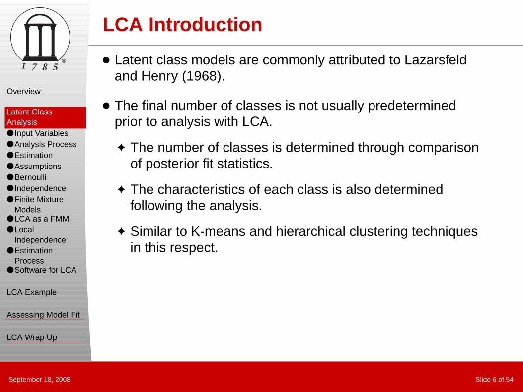
Latent Class Analysis as a FMM

A latent class model for the response vector of J variables(j = 1, . . . , J) with C classes (c = 1, . . . , C):

f(xi) =C

∑

c=1

ηc

J∏

j=1

πxij

jc (1 − πjc)1−xij

● ηc is the probability that any individual is a member of class c

(must sum to one).

● xij is the observed response of individual i to item j.

● πjc is the probability of a positive response to item j from anindividual from class c.

Overview





LCA Example

Assessing Model Fit

LCA Wrap Up

®


LCA Local Independence

● As shown in the LCA distributional form, LCA assumes allBernoulli variables are independent given a class.

✦ This assumption is called Local Independence.

✦ It is also present in many other latent variable modelingtechniques:

■ Item response theory.

■ Factor analysis (with uncorrelated errors).

● What is implied is that any association between observedvariables is accounted for only by the presence of the latentclass.

✦ Essentially, this is saying that the latent class is the reasonthat variables are correlated.

Overview





LCA Example

Assessing Model Fit

LCA Wrap Up

®


Estimation Process

● Successfully applying an LCA model to data involves theresolution to two key questions:

1. How many classes are present?

2. What does each class represent?

● The answer to the first question comes from fitting LCAmodels with differing numbers of classes, then choosing themodel with the best fit (to be defined later).

● The answer to the second question comes from inspectingthe LCA model parameters of the solution that was deemedto have fit best.

Overview





LCA Example

Assessing Model Fit

LCA Wrap Up

®


LCA Estimation Software

● There are several programs that exist that can estimate LCAmodels.

● The package to be used today will be Mplus (with the Mixtureadd-on).

✦ The full version of Mplus is very useful for many statisticaltechniques.

● Other packages also exist:

✦ Latent Gold.

✦ A user-developed procedure in SAS (proc lca).


LCA Example


LCA Example

● To illustrate the process of LCA,we will use the example presentedin Bartholomew and Knott (p. 142).

● The data are from a four-item testanalyzed with an LCA byMacready and Dayton (1977).

● The test data used by Macreadyand Dayton were items from amath test.

● Ultimately, Macready and Dayton wanted to see if examinees could be placedinto two groups:

✦ Those who had mastered the material.

✦ Those who had not mastered the material.

Overview


LCA Example● How Many

Classes● Mplus Syntax● LCA Information● Sample

Information● Item Information● Class

Interpretation

Assessing Model Fit

LCA Wrap Up

®


LCA Example #1

● Several considerations will keep us from assessing thenumber of classes in Macready and Dayton’s data:

✦ We only have four items.

✦ Macready and Dayton hypothesized two distinct classes:masters and non-masters.

● For these reasons, we will only fit the two-class model andinterpret the LCA model parameter estimates.


Mplus Input

TITLE: LCA of Macready and Dayton’s data (1977).Two classes.

DATA: FILE IS mddata.dat;VARIABLE: NAMES ARE u1-u4;

CLASSES = c(2);CATEGORICAL = u1-u4;

ANALYSIS: TYPE = MIXTURE;STARTS = 100 100;

OUTPUT: TECH1 TECH10;PLOT: TYPE=PLOT3;

SERIES IS u1(1) u2(2) u3(3) u4(4);SAVEDATA: FORMAT IS f10.5;

FILE IS examinee_ests.dat;SAVE = CPROBABILITIES;

Overview


LCA Example● How Many

Classes● Mplus Syntax● LCA Information● Sample

Information● Item Information● Class

Interpretation

Assessing Model Fit

LCA Wrap Up

®


LCA Parameter Information Types

● Recall, we have three pieces of information we can gain froman LCA:

✦ Sample information - proportion of people in each class(ηc).

✦ Item information - probability of correct response for eachitem from examinees from each class (πjc).

✦ Examinee information - posterior probability of classmembership for each examinee in each class (αic).


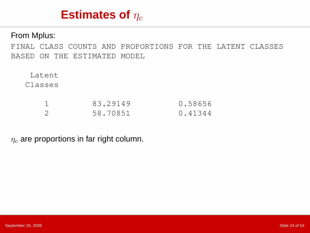
Estimates of ηc

From Mplus:FINAL CLASS COUNTS AND PROPORTIONS FOR THE LATENT CLASSESBASED ON THE ESTIMATED MODEL

LatentClasses

1 83.29149 0.586562 58.70851 0.41344

ηc are proportions in far right column.


Estimates of πjc

From Mplus:RESULTS IN PROBABILITY SCALELatent Class 1U1 Category 2 0.753 0.060U2 Category 2 0.780 0.069U3 Category 2 0.432 0.058U4 Category 2 0.708 0.063

Latent Class 2U1 Category 2 0.209 0.066U2 Category 2 0.068 0.056U3 Category 2 0.018 0.037U4 Category 2 0.052 0.057

πjc are proportions in left column, followed by asymptotic standard errors.


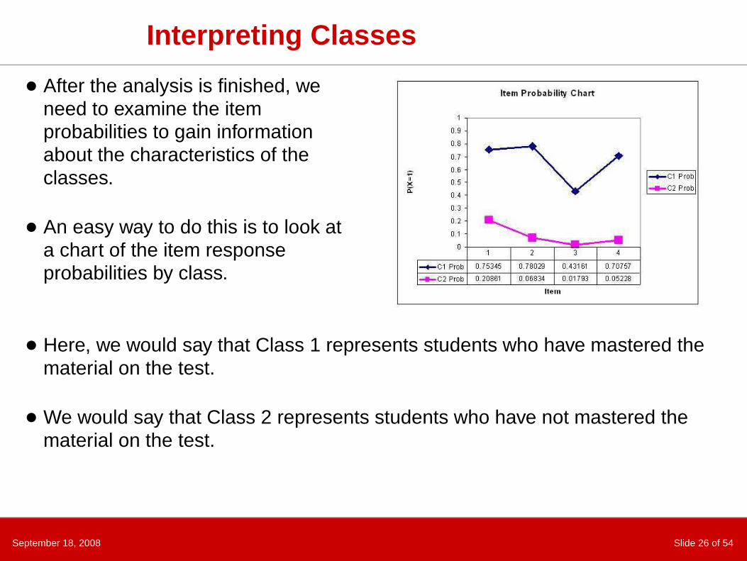
Interpreting Classes

● After the analysis is finished, weneed to examine the itemprobabilities to gain informationabout the characteristics of theclasses.

● An easy way to do this is to look ata chart of the item responseprobabilities by class.

● Here, we would say that Class 1 represents students who have mastered thematerial on the test.

● We would say that Class 2 represents students who have not mastered thematerial on the test.


Assessing Model Fit

Overview


LCA Example

Assessing Model Fit● Model Based

Measures● Model

Chi-squared Test● Likelihood Ratio

Chi-squared● Model

Comparison● Information

Criteria● Distributional

Measures● Entropy

LCA Wrap Up

®


Assessing Model Fit

● As with other statistical techniques, there is no one best wayto assess the fit of an LCA model.

● Techniques typically used can put into several generalcategories:

✦ Model based hypothesis tests (absolute fit).

✦ Information criteria.

✦ Measures based on distributional characteristics.

✦ Entropy.

Overview


LCA Example


Measures● Model





Measures● Entropy

LCA Wrap Up

®


Model Based Measures

● Recall the standard latent class model: Using some notationof Bartholomew and Knott, a latent class model for theresponse vector of p variables (i = 1, . . . , p) with K classes(j = 1, . . . , K):

f(xi) =

K∑

j=1

ηj

p∏

i=1

πxi

ij (1 − πij)1−xi

● Model based measures of fit revolve around the modelfunction listed above.

● With just the function above, we can compute the probabilityof any given response pattern.

● Mplus gives this information using the TECH10 output option.

Overview


LCA Example


Measures● Model





Measures● Entropy

LCA Wrap Up

®


Model Chi-squared Test

● The χ2 test compares the sets of response patterns thatwere observed with the set of response patterns expectedunder the model.

● To form the χ2 test, one must first compute the probability ofeach response pattern using the latent class model equationdisplayed on the last slide.

● The hypothesis tested is that the observed frequency isequal to the expected frequency.

● If the test has a low p-value, the model is said to not fit.

● To demonstrate the model χ2 test, let’s consider the resultsof the latent class model fit to the data from our runningexample (from Macready and Dayton, 1977).

Overview


LCA Example


Measures● Model





Measures● Entropy

LCA Wrap Up

®


Chi-squared Test Example

Class Probabilities:Class Probability1 0.5872 0.413

Item Parametersclass: 1item prob SE(prob)1 0.753 0.0512 0.780 0.0513 0.432 0.0564 0.708 0.054

class: 2item prob SE(prob)1 0.209 0.0602 0.068 0.0483 0.018 0.0294 0.052 0.044

Overview


LCA Example


Measures● Model





Measures● Entropy

LCA Wrap Up

®


Chi-squared Test Example

● To begin, compute the probability of observing the pattern[1111]...

● Then, to find the expected frequency, multiply that probabilityby the number of observations in the sample.

● Repeat that process for all cells...

● The compute χ2p =

∑

r

(Or − Er)2

Er

, where r represents each

response pattern.

● The degrees of freedom are equal to the number of responsepatterns minus model parameters minus one.

● Then find the p-value, and decide if the model fits.


Chi-squared from MplusRESPONSE PATTERN FREQUENCIES AND CHI-SQUARE CONTRIBUTIONS

Response Frequency Standard Chi-square Contribution

Pattern Observed Estimated Residual Pearson Loglikelihood Deleted

1 41.00 41.04 0.01 0.00 -0.08

2 13.00 12.91 0.03 0.00 0.18

3 6.00 5.62 0.16 0.03 0.79

4 7.00 8.92 0.66 0.41 -3.39

5 1.00 1.30 0.27 0.07 -0.53

6 3.00 1.93 0.77 0.59 2.63

7 2.00 2.08 0.05 0.00 -0.15

8 7.00 6.19 0.33 0.10 1.71

9 4.00 4.04 0.02 0.00 -0.07

10 6.00 6.13 0.05 0.00 -0.26

11 5.00 6.61 0.64 0.39 -2.79

12 23.00 19.74 0.79 0.54 7.04

13 4.00 1.42 2.18 4.70 8.29

14 1.00 4.22 1.59 2.46 -2.88

15 4.00 4.90 0.41 0.16 -1.62

16 15.00 14.95 0.01 0.00 0.09

Overview


LCA Example


Measures● Model





Measures● Entropy

LCA Wrap Up

®


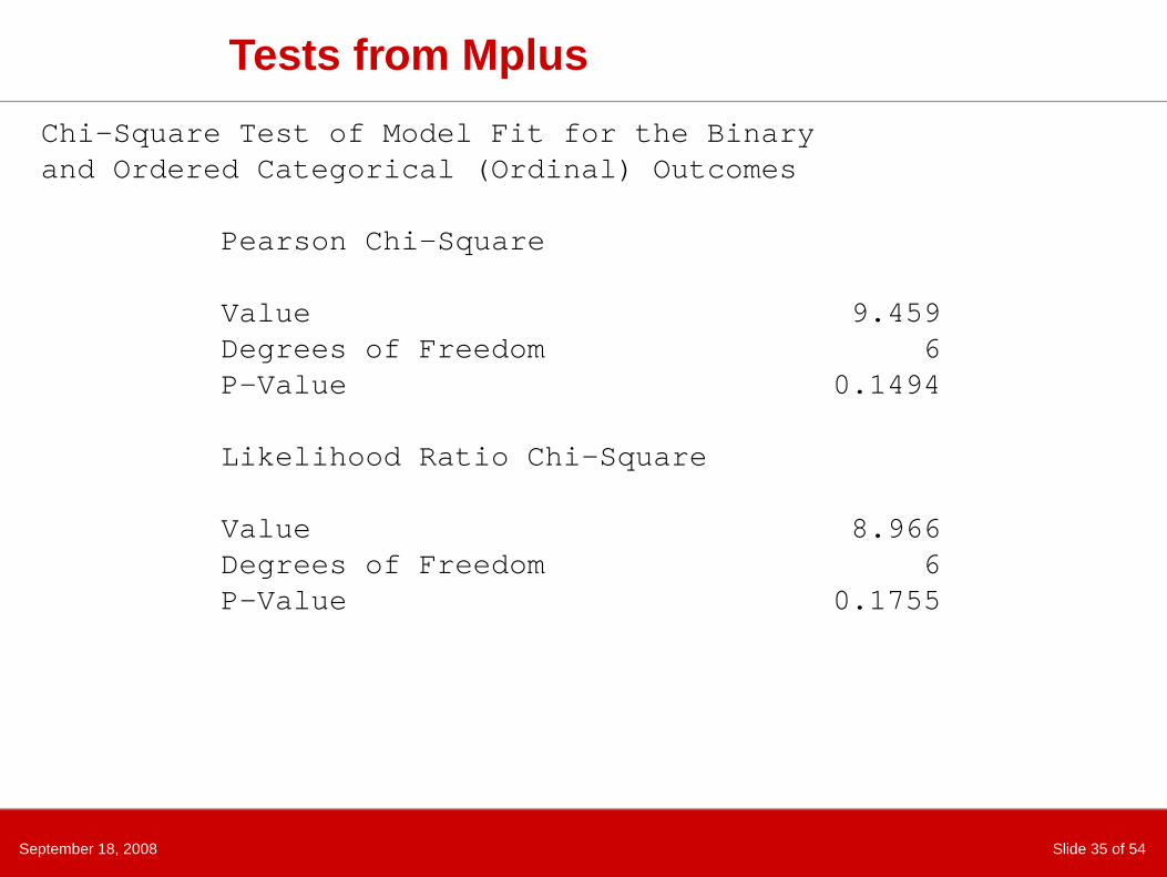
Likelihood Ratio Chi-squared

● The likelihood ratio Chi-square is a variant of the PearsonChi-squared test, but still uses the observed and expectedfrequencies for each cell.

● The formula for this test is:

G = 2∑

r

Or ln

(

Or

Er

)

● The degrees of freedom are still the same as the PearsonChi-squared test, however.


Tests from Mplus

Chi-Square Test of Model Fit for the Binaryand Ordered Categorical (Ordinal) Outcomes

Pearson Chi-Square

Value 9.459Degrees of Freedom 6P-Value 0.1494

Likelihood Ratio Chi-Square

Value 8.966Degrees of Freedom 6P-Value 0.1755

Overview


LCA Example


Measures● Model





Measures● Entropy

LCA Wrap Up

®


Chi-squared Problems

● The Chi-square test is reasonable for situations where thesample size is large, and the number of variables is small.

✦ If there are too many cells where the observed frequencyis small (or zero), the test is not valid.

● Note that the total number of response patterns in an LCA is2J , where J is the total number of variables.

● For our example, we had four variables, so there were 16possible response patterns.

● If we had 20 variables, there would be a total of 1,048,576.

✦ Think about the number of observations you would have tohave if you were to observe at least one person with eachresponse pattern.

✦ Now think about if the items were highly associated (youwould need even more people).

Overview


LCA Example


Measures● Model





Measures● Entropy

LCA Wrap Up

®


Model Comparison

● So, if model-based Chi-squared tests are valid only for alimited set of analyses, what else can be done?

● One thing is to look at comparative measures of model fit.

● Such measures will allow the user to compare the fit of onesolution (say two classes) to the fit of another (say threeclasses).

● Note that such measures are only valid as a means ofrelative model fit - what do these measures become if themodel fits perfectly?

Overview


LCA Example


Measures● Model





Measures● Entropy

LCA Wrap Up

®


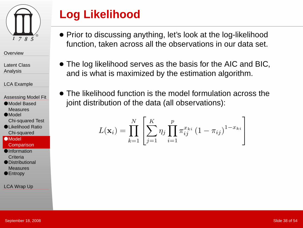
Log Likelihood

● Prior to discussing anything, let’s look at the log-likelihoodfunction, taken across all the observations in our data set.

● The log likelihood serves as the basis for the AIC and BIC,and is what is maximized by the estimation algorithm.

● The likelihood function is the model formulation across thejoint distribution of the data (all observations):

L(xi) =N∏

k=1

K∑

j=1

ηj

p∏

i=1

πxki

ij (1 − πij)1−xki

Overview


LCA Example


Measures● Model





Measures● Entropy

LCA Wrap Up

®


Log Likelihood

● The log likelihood function is the log of the model formulationacross the joint distribution of the data (all observations):

LogL(xi) = log

N∏

k=1

K∑

j=1

ηj

p∏

i=1

πxki


LogL(xi) =N

∑

k=1

log

K∑

j=1

ηj

p∏

i=1

πxki


● Here, the log function taken is typically base e - the naturallog.

● The log likelihood is a function of the observed responses foreach person and the model parameters.

Overview


LCA Example


Measures● Model





Measures● Entropy

LCA Wrap Up

®


Information Criteria

● The Akaike Information Criterion (AIC) is a measure of thegoodness of fit of a model that considers the number ofmodel parameters (q).

AIC = 2q − 2 log L

● Schwarz’s Information Criterion (also called the BayesianInformation Criterion or the Schwarz-Bayesian InformationCriterion) is a measure of the goodness of fit of a model thatconsiders the number of parameters (q) and the number ofobservations (N):

BIC = q log(N) − 2 log L


Fit from Mplus

TESTS OF MODEL FIT

Loglikelihood

H0 Value -331.764


Number of Free Parameters 9Akaike (AIC) 681.527Bayesian (BIC) 708.130Sample-Size Adjusted BIC 679.653(n* = (n + 2) / 24)

Entropy 0.754

Overview


LCA Example


Measures● Model





Measures● Entropy

LCA Wrap Up

®



● When considering which model “fits” the data best, themodel with the lowest AIC or BIC should be considered.

● Although AIC and BIC are based on good statistical theory,neither is a gold standard for assessing which model shouldbe chosen.

● Furthermore, neither will tell you, overall, if your modelestimates bear any decent resemblance to your data.

● You could be choosing between two (equally) poor models -other measures are needed.

Overview


LCA Example


Measures● Model





Measures● Entropy

LCA Wrap Up

®


Distributional Measures of Model Fit

● The model-based Chi-squared provided a measure of modelfit, while narrow in the times it could be applied, that tried tomap what the model said the data looked like to what thedata actually looked like.

● The same concept lies behind the ideas of distributionalmeasures of model fit - use the parameters of the model to“predict” what the data should look like.

● In this case, measures that are easy to attain are measuresthat look at:

✦ Each variable marginally - the mean (or proportion).

✦ The bivariate distribution of each pair of variables -contingency tables (for categorical variables), correlationmatrices, or covariance matrices.

Overview


LCA Example


Measures● Model





Measures● Entropy

LCA Wrap Up

®


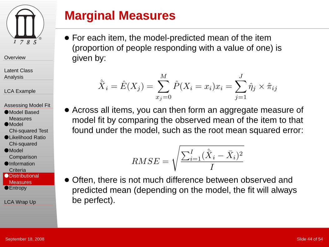
Marginal Measures

● For each item, the model-predicted mean of the item(proportion of people responding with a value of one) isgiven by:

ˆXi = E(Xj) =M∑

xj=0

P (Xi = xi)xi =J

∑

j=1

ηj × πij

● Across all items, you can then form an aggregate measure ofmodel fit by comparing the observed mean of the item to thatfound under the model, such as the root mean squared error:

RMSE =

√

∑I

i=1(ˆXi − Xi)2

I

● Often, there is not much difference between observed andpredicted mean (depending on the model, the fit will alwaysbe perfect).


Marginal Measures from Mplus

From Mplus (using TECH10):UNIVARIATE MODEL FIT INFORMATION

Estimated ProbabilitiesVariable H1 H0 Standard ResidualU1Category 1 0.472 0.472 0.000Category 2 0.528 0.528 0.000

U2Category 1 0.514 0.514 0.000Category 2 0.486 0.486 0.000




Bivariate Measures

● For each pair of items (say a and b, the model-predicted probability of bothbeing one is given in the same way:

P (Xa = 1, Xb = 1) =

J∑

j=1

ηj × πaj × πbj

● Given the marginal means, you can now form a 2 x 2 table of the probabilityof finding a given pair of responses to variable a and b:

ab 0 1

0 1 − P (Xb = 1)

1 P (Xa = 1, Xb = 1) P (Xb = 1)

1 − P (Xa = 1) P (Xa = 1) 1

Overview


LCA Example


Measures● Model





Measures● Entropy

LCA Wrap Up

®


Bivariate Measures

● Given the model-predicted contingency table (on the lastslide) for every pair of items, you can then form a measure ofassociation for the items.

● There are multiple ways to summarize association in acontingency table.

● Depending on your preference, you could use:

✦ Pearson correlation.

✦ Tetrachoric correlation.

✦ Cohen’s kappa.

● After that, you could then summarize the discrepancybetween what your model predicts and what you haveobserved in the data.

✦ Such as the RMSE, MAD, or BIAS.


Bivariate Measures from Mplus

From Mplus (using TECH10):BIVARIATE MODEL FIT INFORMATION

Estimated Probabilities

Variable Variable H1 H0 Standard Residual

U1 U2

Category 1 Category 1 0.352 0.337 0.391

Category 1 Category 2 0.120 0.135 -0.540

Category 2 Category 1 0.162 0.177 -0.483

Category 2 Category 2 0.366 0.351 0.387

Overview


LCA Example


Measures● Model





Measures● Entropy

LCA Wrap Up

®


Entropy

● The entropy of a model is defined to be a measure ofclassification uncertainty.

● To define the entropy of a model, we must first look at theposterior probability of class membership, let’s call this αic

(notation borrowed from Dias and Vermunt, date unknown -online document).

● Here, αic is the estimated probability that observation i is amember of class c

● The entropy of a model is defined as:

EN(α) = −N

∑

i=1

J∑

j=1

αij log αij

Overview


LCA Example


Measures● Model





Measures● Entropy

LCA Wrap Up

®


Relative Entropy

● The entropy equation on the last slide is bounded from[0,∞), with higher values indicated a larger amount ofuncertainty in classification.

● Mplus reports the relative entropy of a model, which is arescaled version of entropy:

E = 1 −EN(α)

N log J

● The relative entropy is defined on [0, 1], with values near oneindicating high certainty in classification and values nearzero indicating low certainty.


Fit from Mplus

TESTS OF MODEL FIT

Loglikelihood

H0 Value -331.764


Number of Free Parameters 9Akaike (AIC) 681.527Bayesian (BIC) 708.130Sample-Size Adjusted BIC 679.653(n* = (n + 2) / 24)

Entropy 0.754


Latent Class Analysis: Wrap Up

Overview


LCA Example

Assessing Model Fit

LCA Wrap Up● Limitations

®


LCA Limitations

● LCA has limitations which can make its general applicationdifficult:

✦ Classes not known prior to analysis.

✦ Class characteristics not know until after analysis.

● Both of these problems are related to LCA being anexploratory procedure for understanding data.

● Diagnostic classification models can be thought of as aconfirmatory versions of LCA.

✦ By placing constraints on the class item probabilities andspecifying what our classes mean prior to analysis.

Overview


LCA Example

Assessing Model Fit

LCA Wrap Up● Limitations

®


LCA Summary

● Latent class analysis is a model-based technique for findingclusters in binary (categorical) data.

● Each of the variables is assumed to:

✦ Have a Bernoulli distribution.

✦ Be independent given class.

● Additional reading: Lazarsfeld and Henry (1968). Latentstructure analysis.

Documents

Latent Class Analysis - Jonathan Templin's Website theory ... Much less often, latent class analysis is included in the group. ... a binary-response item,X