Latent class analysis, Bayesian

statistics and the hidden perils of

test validation studies

Lesley Stringer

Zero-inflated random effect Bayesian test evaluation of individual faecal culture and ELISA to detect

Mycobacterium avium subsp. paratuberculosis infection in young farmed deer

L Stringer1, C Jewell2, C Heuer1, P Wilson1, G Jones1, A Noble1, W Johnson3

1 Massey University 2University of Warwick, 3University of California

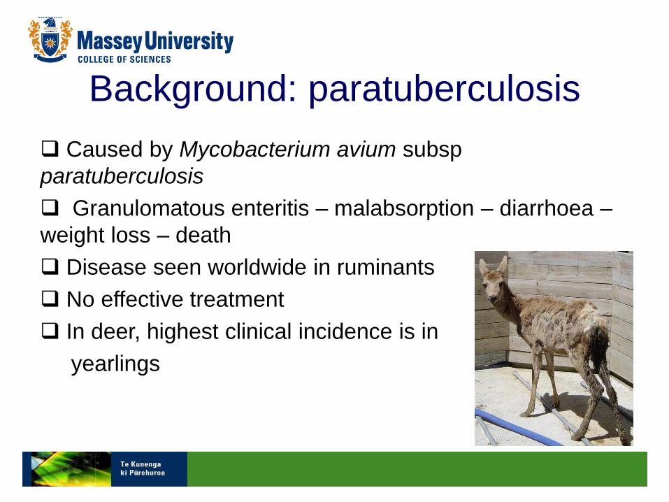
Background: paratuberculosis

Caused by Mycobacterium avium subsp

paratuberculosis

Granulomatous enteritis – malabsorption – diarrhoea –

weight loss – death

Disease seen worldwide in ruminants

No effective treatment

In deer, highest clinical incidence is in

yearlings

The problem

Want to estimate sensitivity and specificity of

individual faecal culture (IFC) and a serum ELISA test

for paratuberculosis in deer

There is no „gold standard‟ test in the live animal

Traditional gold standard

methods

In practice: no perfectly sensitive and specific ante-

mortem test exists for any disease

In theory: error-free diagnostic method which

determines whether the target condition (e.g.

disease/infection) is present or not

Results from test under evaluation are compared to

panel of “true cases” or “true non-cases” to derive

sensitivity and specificity values

Latent class analysis

True disease/infection status of individual is

accepted as unknown (latent)

Test accuracy is derived mathematically

from test results using maximum likelihood

methods or Bayesian inference

Advantages of latent class analysis

Avoids selection of panel of “true positives” biased to

those positive to a gold standard

New test for evaluation may be more sensitive than the

existing gold standard

If Bayesian methods are used to fit the model, smaller

sample size needed

Two test-two population method

First described by Hui and Walter (1980)*

“If two tests are applied simultaneously to the same individuals

from two populations with different disease prevalences, then

assuming conditional independence of the errors of the two tests,

the error rates of both tests and the true prevalences in both

populations can be estimated by a maximum likelihood

procedure”.

* S.L.Hui, S.D. Walter, Biometrics 36, 167-171

Two-test, two population model

assumptions

Test sensitivity and specificity are constant

across populations

The disease prevalences of the two

populations are distinct

Solving the equations

Modelling can be done using maximum

likelihood methods: Newton-Raphson or EM

(expected maximization) algorithms

On-line tools for analysis: TAGS software

Solving the equations

www.epi.ucdavis.edu/diagnostictests

Bayesian latent class analysis Modelling can also be done using Bayesian inference

Bayes theorem

Rev Thomas Bayes, 1702-1761

In words.. Bayes theorem

To get the posterior probability, multiply the prior

probability distribution by the likelihood function

and then normalize.

In words.. Bayes theorem

So in a test validation study we use prior

information on test performance and

prevalence and combine that with the data

(the test results) to derive the posterior

probability for each parameter

The mean, median or mode of the posterior

distribution can be considered the

parameter estimate

Probability or credible intervals i.e. the

interval within which the true value lies with

95% probability are derived by Monte Carlo

simulation from the posterior distribution

Bayesian latent class analysis

The prior probability distribution allows us to

incorporate existing scientific information on each

parameter. Using estimates from prevalence studies,

for example as prior information for the prevalence

parameter.

Can also use expert opinion where no data exists.

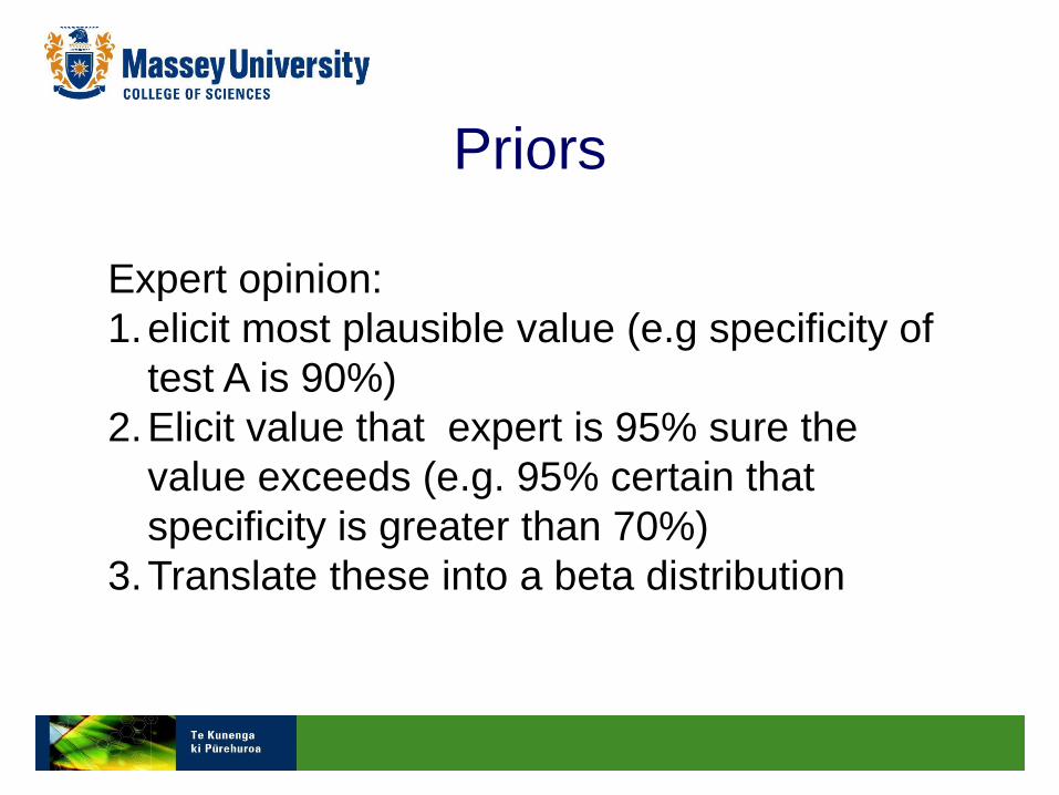
Priors

Expert opinion:

1.elicit most plausible value (e.g specificity of

test A is 90%)

2.Elicit value that expert is 95% sure the

value exceeds (e.g. 95% certain that

specificity is greater than 70%)

3.Translate these into a beta distribution

Betabuster

BetaBuster, University of California, Davis

Prior values

Parameter Prior estimate 5th/95th percentile

Herd prevalence North Island 0.50 >0.1

Herd prevalence South Island 0.70 >0.5

Sensitivity faecal culture 0.50 >0.2

Sensitivity ELISA 0.77 >0.1

Specificity faecal culture 0.98 >0.95

Specificity ELISA 0.995 >0.95

Within-herd prevalence 0.30 <0.9

Two tests two population method

For each population, test results are cross-

classified in the appropriate 2 x 2 table

Population 1

Test 2 + Test 2-

Population 2

Test 2 + Test 2 -

a b

c d

Test 1 +

Test 1 -

e f

g h

Test 1 +

Test 1 -

n1 n2

Latent class analysis

For each cell a-h, equations are derived:

e.g. test result in cell "a" (i.e. positive on both tests)

could occur if the individual is infected, i.e.

true positive

= pi1*se1*se2

or

false positive = (1-pi1)* (1-sp1)*(1-sp2)

a b

c d

Test 1 +

Test 1 -

Test 2+ Test 2 - Pop 1

Latent class analysis

So for cell “a” the likelihood equation is based

on the sum of these probabilities, i.e. true

positive + false positive

a = pi1se1se2 + (1-pi1)(1-sp1)(1-sp2)

Likelihoods for remaining cells are constructed

similarly

Latent class analysis

Cell (a): pi1se1se2 + (1-pi1)(1-sp1)(1-sp2)

Cell (b): pi1se1(1-se2) + (1-pi1)(1-sp1)sp2

Cell (c): pi1(1-se1)se2 + (1-pi1)sp1(1-sp2)

Cell (d): pi1(1-se1)(1-se2) + (1-pi1)sp1sp2

Cell (e): pi2se1se2 + (1-pi2)(1-sp1)(1-sp2)

Cell (f): pi2se1(1-se2) + (1-pi2)(1-sp1)sp2

Cell (g): pi2(1-se1)se2+ (1-pi2)sp1(1-sp2)

Cell (h): pi2(1-se1)(1-se2) + (1-pi2)sp1sp2

These are the equations to be solved:

Latent class analysis

Six parameters can be estimated from the observed data:

prevalence in pop‟n 1 (pi1) and pop‟n 2 (pi2)

sensitivity of ELISA (se1) and culture (se2)

specificity of ELISA (sp1) and culture (sp2)

Back to the study question

Test validation: should consider

1. Test purpose (confirmation of diagnosis? Freedom

from disease? Test and cull?)

2. Target condition (Infected? Infectious? Clinically

diseased?)

3. Target population

Estimate the sensitivity and specificity of two diagnostic

tests (IFC and ELISA) for paratuberculosis

The study question

Estimate the sensitivity and specificity of IFC and ELISA to

identify clinically normal yearling deer infected with MAP for

the purpose of herd classification (freedom from disease

sampling)

Study design

20 clinically normal yearling deer sampled

(faeces and blood) in 20 herds SI, 18 NI

Prevalence of MAP infection in farmed deer

different in North (29%) and South Island

(51%) of New Zealand – two populations

Results for each animal of individual faecal

culture and a serum IgG1ELISA

1200000 1600000 2000000

50

00

00

05

50

00

00

60

00

00

0

2000

5500

5700

5900

6100

sampled herds

Statistical problems

Samples not independent observations,

clustered in herds

Variation in within-herd prevalence expected

Possibility of non-infected herds

Solution: extended HW model

Variation in within-herd prevalence modelled

as a random effect

Zero-inflation effect incorporated, allowing

modelling to include probability of herd being

non-infected

Practical problems

Important that vets collect samples to minimise

cross-contamination

“I use a spoon for faeces collection but wash it between bums so it is

clean. And gloves cost money too!”

Clear instructions to use fresh gloves each sample

Test run of questionnaire, instructions and sampling

To be sure, to be sure….contact each vet post-

sampling

Results from IFC and ELISA

757 paired samples:

401 from the South Island

356 from the North island

North Island

IFC + IFC-

1 15

1 339

10 27

45 319 ELISA -

ELISA +

South Island

IFC + IFC -

Herd-level results

05

10

15

20

05

10

15

20

North Island

South Island

Faecal culture Paralisa

Test p

ositiv

e (

n)

Herd

IFC pos = 2 herds in NI, 8 herds SI

ELISA pos = 8 herds NI, 13 SI

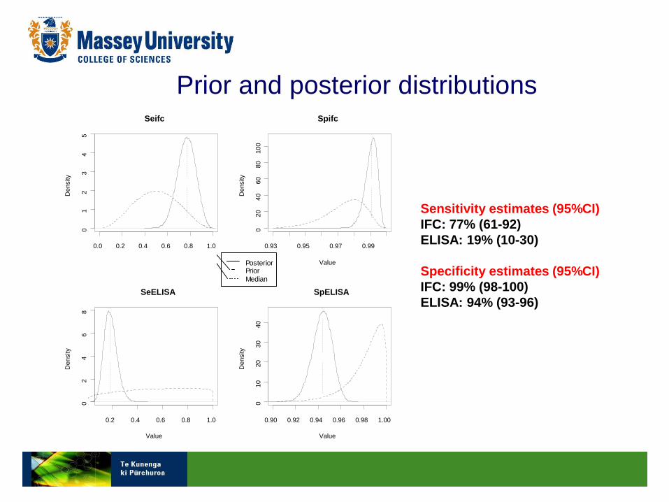
Prior and posterior distributions

PosteriorPrior

Median

Sensitivity estimates (95%CI)

IFC: 77% (61-92)

ELISA: 19% (10-30)

Specificity estimates (95%CI)

IFC: 99% (98-100)

ELISA: 94% (93-96)

0.0 0.2 0.4 0.6 0.8 1.0

0

1

2

3

4

5

Seifc

Density

0.93 0.95 0.97 0.99

0

20

40

60

80

100

Spifc

Value

Density

0.2 0.4 0.6 0.8 1.0

0

2

4

6

8

SeELISA

Value

Density

0.90 0.92 0.94 0.96 0.98 1.00

0

10

20

30

40

SpELISA

Value

Density

Sensitivity analysis

Model run changing priors for herd prevalence,

within-herd prevalence, using pessimistic test sensitivity

and specificity priors:

Little effect on posterior distributions

Conclusion: model robust to changes in prior

information, i.e. estimates driven by the data rather

than the priors

Example sensitivity analysis (red = changed value)

Parameter Median SD 2.5%

quantile 97.5% quantile

Sensitivity IFC 0.77 0.08 0.61 (0.92)

Sensitivity ELISA 0.18 (0.19) 0.05 0.10 0.30

Specificity IFC 0.99 0.004 0.98 1.00

Specificity ELISA 0.94 0.009 0.92 (0.93) 0.95 (0.96)

Original prior for SP ELISA: most likely value = 99.5%

(95% certain that greater than 95%)

Amend prior for SP ELISA to 90% (95% certain that greater than 20%)

Back to the question

Estimate the sensitivity and specificity IFC and ELISA to identify

clinically normal yearling deer infected with MAP for the purpose

of herd classification (freedom from infection sampling)

So…

Applied two tests in two populations of different prevalence

Used latent class analysis, i.e. non-gold standard method

Taken into account that herds may not be infected (zero-

inflation) and modelled the within-herd prevalence using a

random-effects logistic model

Used Bayesian inference to derive the sensitivity and

specificity estimates

Conclusion

IFC is more sensitive (77% vs 19%) and specific (99% vs

94%) at the individual level than ELISA in yearling deer in New

Zealand

Prior values Derived from published literature:

Se IFC: 50% (95% certain that >20%)

Se ELISA: 77% (95% certain that >10%)

Sp IFC: 98% (95% certain that >95%)

Sp ELISA: 99.5% (95% certain that >95%)

Posterior values of test performance

Se IFC: 77% (95CI 60%-92%)

Se ELISA: 19% (95%CI 10% - 30%)

Sp IFC: 99% (95%CI 98%-99.7%)

Sp ELISA: 94% (95% CI 93%-96%)

What happened next?

Some comments…

…in analyses like this it is not uncommon to drop extreme

results that do not appear to be biologically sensible .

….the analysis is likely to have been greatly biased by just

two herds which

(a) are “outliers”

(b) are not biologically plausible; and/or

(c) do not have an explanation with our current knowledge.

Removing data?

05

10

15

20

05

10

15

20

North Island

South Island

Faecal culture Paralisa

Test p

ositiv

e (

n)

Herd

A B

Removing data?

Results of analysis excluding herd A (15 IFC +, no ELISA +)

Parameter Median 95% CI

SeIFC 0.76 0.56 - 0.92

Separa 0.27 0.15 - 0.41

SpIFC 0.99 0.98 - 0.997

Sppara 0.94 0.93 - 0.96

Excluding herd B (17 IFC +, 2 ELISA +)

Parameter Median 95% CI

SeIFC 0.69 0.47- 0.89

Separa 0.22 0.11- 0.36

SpIFC 0.99 0.98- 0.997

Sppara 0.94 0.93- 0.96

Excluding both herds

Parameter Median 95% CI

SeIFC 0.51 0.27- 0.82

Separa 0.39 0.22- 0.60

SpIFC 0.99 0.98-0.997

Sppara 0.95 0.93- 0.97

Full model estimates

Sensitivity (95%CI)

IFC: 77% (61-92)

ELISA: 19% (10-30)

Specificity (95%CI)

IFC: 99% (98-100)

ELISA: 94% (93-96)

WINbugs code # Population 1

for (i in 1:ny1) {

myN1[i] <- y1[i,1] + y1[i,2] + y1[i,3] + y1[i,4]

y1[i,1:4] ˜ dmulti(p1[i,1:4], myN1[i])

p1[i,1] <- pi1[i]*SeELISA*Seifc + (1-pi1[i])*(1-SpELISA)*(1-Spifc)

p1[i,2] <- pi1[i]*SeELISA*(1-Seifc) + (1-pi1[i])*(1-SpELISA)*Spifc

p1[i,3] <- pi1[i]*(1-SeELISA)*Seifc + (1-pi1[i])*SpELISA*(1-Spifc)

p1[i,4] <- pi1[i]*(1-SeELISA)*(1-Seifc) + (1-pi1[i])*SpELISA*Spifc

pi1[i] <- z1[i] * pistar1[i]

z1[i] ˜ dbern(phi1)

logit(pistar1[i]) <- alpha + U1[i]

U1[i] ˜ dnorm(0, tau)

}

# Population 2

for (i in 1:ny2) {

myN2[i] <- y2[i,1] + y2[i,2] + y2[i,3] + y2[i,4]

y2[i,1:4] ˜ dmulti(p2[i,1:4], myN2[i])

p2[i,1] <- pi2[i]*SeELISA*Seifc + (1-pi2[i])*(1-SpELISA)*(1-Spifc)

p2[i,2] <- pi2[i]*SeELISA*(1-Seifc) + (1-pi2[i])*(1-SpELISA)*Spifc

p2[i,3] <- pi2[i]*(1-SeELISA)*Seifc + (1-pi2[i])*SpELISA*(1-Spifc)

p2[i,4] <- pi2[i]*(1-SeELISA)*(1-Seifc) + (1-pi2[i])*SpELISA*Spifc

pi2[i] <- z2[i] * pistar2[i]

z2[i] ~ dbern(phi2)

logit(pistar2[i]) <- alpha + U2[i]

U2[i] ~ dnorm(0,tau)

}