Technical ReportNumber 724

Computer Laboratory

UCAM-CL-TR-724ISSN 1476-2986

Bayesian inference forlatent variable models

Ulrich Paquet

July 2008

15 JJ Thomson Avenue

Cambridge CB3 0FD

United Kingdom

phone +44 1223 763500

http://www.cl.cam.ac.uk/

c© 2008 Ulrich Paquet

This technical report is based on a dissertation submittedMarch 2007 by the author for the degree of Doctor ofPhilosophy to the University of Cambridge, Wolfson College.

Technical reports published by the University of CambridgeComputer Laboratory are freely available via the Internet:

http://www.cl.cam.ac.uk/techreports/

ISSN 1476-2986

Abstract 3

Abstract

Bayes’ theorem is the cornerstone of statistical inference. It provides the tools for dealing withknowledge in an uncertain world, allowing us to explain observed phenomena through the re-finement of belief in model parameters. At the heart of this elegant framework lie intractableintegrals, whether in computing an average over some posterior distribution, or in determin-ing the normalizing constant of a distribution. This thesis examines both deterministic andstochastic methods in which these integrals can be treated. Of particular interest shall be para-metric models where the parameter space can be extended with additional latent variables toget distributions that are easier to handle algorithmically.

Deterministic methods approximate the posterior distribution with a simpler distributionover which the required integrals become tractable. We derive and examine a new genericα-divergence message passing scheme for a multivariate mixture of Gaussians, a particular mod-eling problem requiring latent variables. This algorithm minimizes local α-divergences over achosen posterior factorization, and includes variational Bayes and expectation propagation asspecial cases.

Stochastic (or Monte Carlo) methods rely on a sample from the posterior to simplify theintegration tasks, giving exact estimates in the limit of an infinite sample. Parallel temper-ing and thermodynamic integration are introduced as ‘gold standard’ methods to sample frommultimodal posterior distributions and determine normalizing constants. A parallel temperedapproach to sampling from a mixture of Gaussians posterior through Gibbs sampling is de-rived, and novel methods are introduced to improve the numerical stability of thermodynamicintegration. A full comparison with parallel tempering and thermodynamic integration showsvariational Bayes, expectation propagation, and message passing with the Hellinger distanceα = 1

2 to be perfectly suitable for model selection, and for approximating the predictive distri-bution with high accuracy.

Variational and stochastic methods are combined in a novel way to design Markov chainMonte Carlo (MCMC) transition densities, giving a variational transition kernel, which lowerbounds an exact transition kernel. We highlight the general need to mix variational methodswith other MCMC moves, by proving that the variational kernel does not necessarily give ageometrically ergodic chain.

4 Acknowledgments

Acknowledgments

My time in Cambridge was generously supported by the Association of Commonwealth Univer-sities through a Commonwealth Scholarship, for which I am deeply thankful.

Numerous people have been instrumental in the way I think about inference, and I thankOle Winther for great collaboration and support, and for hosting me for a week at the TechnicalUniversity of Denmark, Tom Minka and Martin Szummer for organizing the reading group atMicrosoft Research, and David MacKay and the Inference group at the Cavendish Laboratoryfor providing a platform for many stimulating talks. At the Computer Laboratory I thank SeanHolden for allowing me the freedom to satisfy my curiosity, and Andrew Naish-Guzman for beinga fantastic labmate, conference partner and friend. I had the best of times working on some oddprojects: with Joseph Stevick on Gaussian Processes to correct MRI images, and with BlaiseThomson on collaborative filtering.

At College I thank a group of great friends, especially Joseph Stevick, Blaise Thomson,Muzoora Bishanga, Glenton and Christine Jelbert, Heather Harrison, Werner Baumker, andGerhard Hancke. Thanks also to my teammates at Cambridge University Hare & Hounds.

Further from Cambridge I thank my family at home, who have given me tremendous en-couragement throughout my graduate years.

Ulrich Paquet, Cambridge, March 2007

Contents

Abstract . . . . . . . . . . . . . . . . . . . . . . . . . . . . . . . . . . . . . . . . . . . . 3

Acknowledgments . . . . . . . . . . . . . . . . . . . . . . . . . . . . . . . . . . . . . . . 4

1 Introduction 9

1.1 Learning from data . . . . . . . . . . . . . . . . . . . . . . . . . . . . . . . . . . . 9

1.2 Bayes’ theorem . . . . . . . . . . . . . . . . . . . . . . . . . . . . . . . . . . . . . 10

1.2.1 Prediction . . . . . . . . . . . . . . . . . . . . . . . . . . . . . . . . . . . . 10

1.2.2 Marginalization . . . . . . . . . . . . . . . . . . . . . . . . . . . . . . . . . 10

1.2.3 Model selection . . . . . . . . . . . . . . . . . . . . . . . . . . . . . . . . . 11

1.3 Practical approaches . . . . . . . . . . . . . . . . . . . . . . . . . . . . . . . . . . 12

1.3.1 Deterministic methods . . . . . . . . . . . . . . . . . . . . . . . . . . . . . 13

1.3.2 Stochastic (Monte Carlo) methods . . . . . . . . . . . . . . . . . . . . . . 15

1.4 Latent variable models . . . . . . . . . . . . . . . . . . . . . . . . . . . . . . . . . 17

1.4.1 Mixtures of distributions . . . . . . . . . . . . . . . . . . . . . . . . . . . . 18

1.4.2 Gibbs sampling and latent variable models . . . . . . . . . . . . . . . . . 19

1.4.3 Variational Bayes and latent variable models . . . . . . . . . . . . . . . . 19

1.5 Conclusion and summary of the remaining chapters . . . . . . . . . . . . . . . . . 20

2 Deterministic Approximate Inference 25

2.1 Introduction . . . . . . . . . . . . . . . . . . . . . . . . . . . . . . . . . . . . . . . 25

2.2 Divergence measures . . . . . . . . . . . . . . . . . . . . . . . . . . . . . . . . . . 26

2.3 A simple mixture of Gaussians . . . . . . . . . . . . . . . . . . . . . . . . . . . . 29

2.4 Expectation propagation: a single observation . . . . . . . . . . . . . . . . . . . . 30

2.4.1 The scale . . . . . . . . . . . . . . . . . . . . . . . . . . . . . . . . . . . . 31

2.4.2 Parameter updates for the components . . . . . . . . . . . . . . . . . . . . 31

2.5 Variational Bayes: a single observation . . . . . . . . . . . . . . . . . . . . . . . . 32

2.5.1 Parameter updates . . . . . . . . . . . . . . . . . . . . . . . . . . . . . . . 32

2.5.2 The scale . . . . . . . . . . . . . . . . . . . . . . . . . . . . . . . . . . . . 33

2.6 α-divergence: a single observation . . . . . . . . . . . . . . . . . . . . . . . . . . . 34

2.6.1 Fixed point iterations . . . . . . . . . . . . . . . . . . . . . . . . . . . . . 35

2.7 Minimizing over a factor graph . . . . . . . . . . . . . . . . . . . . . . . . . . . . 37

2.7.1 A generic message passing algorithm . . . . . . . . . . . . . . . . . . . . . 38

2.7.2 Minimizing the mixtures example over a factor graph . . . . . . . . . . . 39

2.8 Model pruning . . . . . . . . . . . . . . . . . . . . . . . . . . . . . . . . . . . . . 41

2.9 The objective function . . . . . . . . . . . . . . . . . . . . . . . . . . . . . . . . . 43

2.9.1 The objective function for α 6= 0 . . . . . . . . . . . . . . . . . . . . . . . 44

2.9.2 The VB objective function . . . . . . . . . . . . . . . . . . . . . . . . . . 47

2.9.3 Message passing with α = 0 as an EM algorithm . . . . . . . . . . . . . . 49

6 Contents

2.10 Summary . . . . . . . . . . . . . . . . . . . . . . . . . . . . . . . . . . . . . . . . 53

3 Approximate inference for multivariate mixtures 55

3.1 Introduction . . . . . . . . . . . . . . . . . . . . . . . . . . . . . . . . . . . . . . . 55

3.2 Mixture of Gaussians . . . . . . . . . . . . . . . . . . . . . . . . . . . . . . . . . . 56

3.3 Expectation propagation: a single observation . . . . . . . . . . . . . . . . . . . . 57

3.3.1 The scale . . . . . . . . . . . . . . . . . . . . . . . . . . . . . . . . . . . . 58

3.3.2 Parameter updates for the components . . . . . . . . . . . . . . . . . . . . 58

3.3.3 Parameter updates for the mixing weights . . . . . . . . . . . . . . . . . . 60

3.4 Variational Bayes: a single observation . . . . . . . . . . . . . . . . . . . . . . . . 61

3.4.1 Parameter updates . . . . . . . . . . . . . . . . . . . . . . . . . . . . . . . 61

3.4.2 The scale . . . . . . . . . . . . . . . . . . . . . . . . . . . . . . . . . . . . 62

3.5 α-divergence: a single observation . . . . . . . . . . . . . . . . . . . . . . . . . . . 63

3.5.1 Fixed point iterations . . . . . . . . . . . . . . . . . . . . . . . . . . . . . 64

3.6 Minimizing over a factor graph . . . . . . . . . . . . . . . . . . . . . . . . . . . . 67

3.7 Experimental results . . . . . . . . . . . . . . . . . . . . . . . . . . . . . . . . . . 70

3.7.1 A toy example . . . . . . . . . . . . . . . . . . . . . . . . . . . . . . . . . 70

3.7.2 Experimental observations . . . . . . . . . . . . . . . . . . . . . . . . . . . 70

3.7.3 The predictive distribution . . . . . . . . . . . . . . . . . . . . . . . . . . 74

3.7.4 Ockham hills and the approximate log marginal likelihood . . . . . . . . . 74

3.8 Summary and outlook . . . . . . . . . . . . . . . . . . . . . . . . . . . . . . . . . 80

3.8.1 Hidden Markov models . . . . . . . . . . . . . . . . . . . . . . . . . . . . 80

3.8.2 Latent variable models requiring further approximations . . . . . . . . . . 81

3.8.3 Perturbative corrections . . . . . . . . . . . . . . . . . . . . . . . . . . . . 82

4 Parallel Tempering 85

4.1 Introduction . . . . . . . . . . . . . . . . . . . . . . . . . . . . . . . . . . . . . . . 85

4.1.1 Replicas at temperatures . . . . . . . . . . . . . . . . . . . . . . . . . . . 85

4.1.2 Extended ensembles and replica exchange . . . . . . . . . . . . . . . . . . 86

4.1.3 Choosing a temperature set . . . . . . . . . . . . . . . . . . . . . . . . . . 87

4.2 Thermodynamic integration and the marginal likelihood . . . . . . . . . . . . . . 88

4.2.1 The correct interpolation, or glitches at β ≈ 0 . . . . . . . . . . . . . . . . 89

4.3 A practical generalization of parallel tempering . . . . . . . . . . . . . . . . . . . 91

4.4 Gibbs sampling for parallel tempering . . . . . . . . . . . . . . . . . . . . . . . . 92

4.4.1 Gibbs sampling at β . . . . . . . . . . . . . . . . . . . . . . . . . . . . . . 92

4.4.2 Gibbs sampling at β for generalized parallel tempering . . . . . . . . . . . 94

4.5 Experimental results . . . . . . . . . . . . . . . . . . . . . . . . . . . . . . . . . . 95

4.6 Discussion: annealed importance sampling . . . . . . . . . . . . . . . . . . . . . . 96

4.7 Summary and outlook . . . . . . . . . . . . . . . . . . . . . . . . . . . . . . . . . 97

4.7.1 Other MCMC schemes . . . . . . . . . . . . . . . . . . . . . . . . . . . . . 97

4.7.2 Choices for q(θ) . . . . . . . . . . . . . . . . . . . . . . . . . . . . . . . . 97

5 Variational Transition Kernels 101

5.1 Introduction . . . . . . . . . . . . . . . . . . . . . . . . . . . . . . . . . . . . . . . 101

5.2 Monte Carlo methods . . . . . . . . . . . . . . . . . . . . . . . . . . . . . . . . . 102

5.2.1 Monte Carlo integration . . . . . . . . . . . . . . . . . . . . . . . . . . . . 102

5.2.2 Markov chains . . . . . . . . . . . . . . . . . . . . . . . . . . . . . . . . . 102

5.2.3 Metropolis-Hastings . . . . . . . . . . . . . . . . . . . . . . . . . . . . . . 105

Contents 7

5.3 Variational transition kernel . . . . . . . . . . . . . . . . . . . . . . . . . . . . . . 1075.3.1 An exact transition kernel . . . . . . . . . . . . . . . . . . . . . . . . . . . 1075.3.2 A tractable approximation . . . . . . . . . . . . . . . . . . . . . . . . . . . 1085.3.3 Illustrative example: Mixture of distributions . . . . . . . . . . . . . . . . 109

5.4 Using the proposal in Monte Carlo methods . . . . . . . . . . . . . . . . . . . . . 1105.4.1 Toy example . . . . . . . . . . . . . . . . . . . . . . . . . . . . . . . . . . 1105.4.2 Importance sampling . . . . . . . . . . . . . . . . . . . . . . . . . . . . . . 1145.4.3 Mixing kernels . . . . . . . . . . . . . . . . . . . . . . . . . . . . . . . . . 117

5.5 Concluding remarks . . . . . . . . . . . . . . . . . . . . . . . . . . . . . . . . . . 117

6 Conclusion 1196.1 Summary of contributions . . . . . . . . . . . . . . . . . . . . . . . . . . . . . . . 1196.2 Future work . . . . . . . . . . . . . . . . . . . . . . . . . . . . . . . . . . . . . . . 120

A Useful results 123A.1 Kullback-Leibler as special cases of an α-divergence . . . . . . . . . . . . . . . . . 123A.2 Responsibility-weighted moment matching: two derivations . . . . . . . . . . . . 123

A.2.1 A Gaussian derivation . . . . . . . . . . . . . . . . . . . . . . . . . . . . . 123A.2.2 A Dirichlet derivation . . . . . . . . . . . . . . . . . . . . . . . . . . . . . 124

A.3 The scale for multivariate mixtures . . . . . . . . . . . . . . . . . . . . . . . . . . 125A.4 α-divergence scales . . . . . . . . . . . . . . . . . . . . . . . . . . . . . . . . . . . 125

A.4.1 For section 2.6: a simple mixture . . . . . . . . . . . . . . . . . . . . . . . 126A.4.2 For section 3.5: a multivariate mixture . . . . . . . . . . . . . . . . . . . . 126

A.5 Multinomial updates for a fixed point scheme . . . . . . . . . . . . . . . . . . . . 128A.6 Normal-Wishart integrals . . . . . . . . . . . . . . . . . . . . . . . . . . . . . . . 129A.7 The matrix inversion lemma . . . . . . . . . . . . . . . . . . . . . . . . . . . . . . 131

Bibliography 133

Chapter 1

Introduction

1.1 Learning from data

Bayesian theory provides a general and consistent framework for dealing with uncertainty. Ineveryday life uncertainty often permeates our choices, and when choices need to be made, pastexperience frequently proves a helpful aid.

This very same principle is applicable when machines are faced with the task of learningand dealing with uncertainty. Learning from past experience may take many guises, of whichclassification, regression and density estimation are but a few. As a practical example, we maycare about the automatic classification of handwritten digits. When given an image of a writtendigit, we wish to predict whether it is a number from zero to nine. This task is simpler ifwe actually know how typical examples are classified, and a helpful aid in this case is a set ofexample classifications, or a data set of labeled images of handwritten digits. Uncertainty canthen be dealt with in a crisp manner: what is the probability that an image corresponds to anine, say, given that we know how a few other images should be classified?

It is impractical to enumerate and store every possible variation of a written digit. There-fore the approach forwarded by machine learning is to assume that some parametric model isresponsible for generating the labels for written digits. This model can be used for predictionof previously unseen digits by tuning its parameters to predict the observed examples well, andwe effectively learn a functional mapping (or model) from an input to an output space. At thecore, we hope to make good predictions in the future by fitting a model to known predictions.As an aside, nothing confines us to use a single model, as the rules of probability advocate anaveraging of predictions over a set of plausible models or possible parameter settings.

In the above example, and also in regression, we are concerned with the probability distribu-tion of an output variable; given some input variable, the output is treated as a random variable.In the same manner the input variable can be treated with uncertainty. In density estimation,we are interested in the unknown distribution from which some data points have been gener-ated. Continuing the same example, we may be presented with an unlabeled set of images ofwritten characters, and asked to infer the probability density of an image of a character, giventhe observations. Again, we would assume some underlying model with tunable parameters todescribe the density well.

10 1. Introduction

1.2 Bayes’ theorem

The problem of learning from data can be cast into a formal Bayesian framework. Say weobserve data x = {xn}Nn=1, or equally say that some observations from a random variable havebeen made. To ‘learn’ from the observed data, or use it for inference, it is necessary to assumethat it was generated by some model M, possibly with parameters θ. A common assumptionis that the data are independent and identically distributed and drawn from some likelihoodp(xn|θ,M). This sets the scene for parametric inference. It is not always necessary to explicitlywork with our model parameters; non-parametric methods can provide for an equally elegantexample of Bayesian inference. Although the methods discussed here are general, all examplesin this thesis come from the parametric camp.

Bayes’ theorem forces us to make our model assumptionsM explicit; in other words, we areasked to specify the model that we believe in. This opens the door for sensibly comparing models,which will be explored later. From Bayes’ theorem the posterior distribution over the parametersis equal to the likelihood of observing that data, given a particular parameter setting, multipliedby our prior belief about the parameter values. This is scaled by a normalizing constant that isknown as the evidence or marginal likelihood,

p(θ|x,M) =p(x,θ|M)

∫p(x,θ|M) dθ

=p(x|θ,M)p(θ|M)

p(x|M). (1.1)

Under the assumption of independent and identically distributed data, the likelihood is a productover individual example likelihoods, p(x|θ,M) =

∏Nn=1 p(xn|θ,M).

Three common tasks of interest are: 1) the prediction of unseen data conditioned on theobserved data, or more generally determining expectations over the posterior distribution; 2)integrating away parameters we are not interested in, also called marginalization; 3) the evalua-tion of the validity of our assumed model, which includes the task of computing the normalizingconstant in Bayes’ theorem.

1.2.1 Prediction

The first question is that of prediction—determining the distribution of a new data point giventhe observed data—and is answered by averaging over the posterior distribution,

p(xnew|x,M) =

∫

p(xnew|θ,M)p(θ|x,M) dθ . (1.2)

This is often a difficult and analytically intractable integration problem, as the posterior mayhave a very convoluted form, often being high-dimensional with many modes. Even more gen-erally we may want to average functions over the posterior with

Φ = 〈φ(θ)〉 =

∫

φ(θ)p(θ|x,M) dθ , (1.3)

which may include determining the posterior mean, with φ(θ) = θ, for example.

1.2.2 Marginalization

If we have a joint distribution over variables θ and z, we may only be interested in the marginaldistribution over θ, and average over the other variables

p(θ|x,M) =

∫

p(θ, z|x,M) dz . (1.4)

1.2. Bayes’ theorem 11

1.2.3 Model selection

The task of estimating the normalizing constant in Bayes’ theorem is related to another questionthat we may ask, namely how well our assumed model supports the data. There is no guaranteethat a specific modelM provides a preferable description of the data, and the road of inferencediverges into two paths—

1. We make the assumption that each model in a set of models {Mi} has some possibilityof generating the data, and make predictions by averaging over the respective posteriordistributions of each Mi.

2. We prefer one model from {Mi}, and base our choice on the marginal likelihood as anatural embodiment of Ockham’s razor.

Both these paths are discussed below.

Averaging over a set of models

Prediction may rely on higher levels of inference, where we average the predictive distributionof equation (1.2) over the posterior distribution of a set of plausible models {Mi}, with

p(xnew|x) =∑

Mi

p(xnew|x,Mi)p(Mi|x) . (1.5)

In each case p(xnew|x,Mi) will involve integration over a set of parameters specific to Mi.For model averaging to be possible, we have to define a prior distribution p(Mi) over the

set of models, and again rely on Bayes’ theorem for the posterior,

p(Mi|x) =p(x|Mi)p(Mi)

p(x). (1.6)

The term ‘marginal likelihood’—the normalizer or evidence from equation (1.1)—is the likelihoodterm in equation (1.6). The likelihood is marginal, as the model parameters are integrated (ormarginalized) out.

Ockham’s razor

In the context of Bayes’ theorem, the question of how well our assumed model supports thedata is answered by the marginal likelihood. This is the question of model selection: we maywant to know how many clusters would be sufficient to model the data well, what the intrinsicdimensionality of the data is, whether an input is relevant to predicting an output, and so forth.

When comparing models M1 and M2 on seeing data x, we consider the probability ratiobetween the posterior probabilities of the two models. From equation (1.6) we have

p(M1|x)

p(M2|x)=p(x|M1)

p(x|M2)

p(M1)

p(M2). (1.7)

When determining the posterior ratio, two ratios are taken into account. A prior ratio p(M1)/p(M2)encodes how much our initial beliefs favor one model over the other. The ratio of marginal like-lihoods p(x|M1)/p(x|M2) gives an indication of how much better one model is in explainingthe data, compared to the other. We may let the prior ratio prefer a simpler model to a morecomplex one, but the beautiful consequence of dealing with uncertainty using Bayesian theoryis that Ockham’s razor is automatically expressed (MacKay, 1992).

The English Franciscan friar William of Ockham is known in the scientific community by hisfamous razor,

12 1. Introduction

p(X|Mi)

p(X|M1)

x X

p(X|M2)

p(X|M3)

Figure 1.1: A schematic illustration of Ockham’s razor. We imagine that all data sets, which we call X ,are projected onto the one-dimensional horizontal axis. X is a random variable, and therefore p(X|Mi)should integrate to one for each model. As a complex model M3 can explain many data sets, it shouldalso spread its probability mass over a large ‘area’ of data sets. Consequently, if a specific data set x isobserved, the most probable model is the model with largest marginal likelihood, i.e. a model that isneither too simple nor too complex for x. This figure is adapted from (MacKay, 1995).

entia non sunt multiplicanda praeter necessitatem,

which translates to “entities should not be multiplied beyond necessity”. It advocates thesimplest possible explanation for the data that we have observed, but no simpler explanationthan that. Figure 1.1 gives a cartoon, illustrating how a simple modelM2 may give a reasonableexplanation to a few data sets, while a complex modelM3 with more parameters may explain awider variety of data sets.1 The probability mass p(X|M3) of the a more complexM3 should bespread over a larger ‘area’ of data sets X . Hence, when a particular data set x can be explainedwell by both models, we observe a higher marginal likelihood for the simpler model. The higherthe marginal likelihood, the better the model supports the data. If we follow the same argumentfor figure 1.1, it is clear why a ‘too simple’ model M1 would also not be preferred. Bayes’theorem provides a natural way of penalizing models with superfluous power of explanationthrough the marginal likelihood.

In both the case of model averaging and model selection through Ockham’s razor, we need todetermine the marginal likelihood. As in the case of prediction, this is often a difficult problem,as evaluation of the integral

∫p(x,θ|M) dθ can be analytically intractable.

1.3 Practical approaches

Many problems in Bayesian inference therefore leave us with intractable questions: we cannotsimply write down the answer in a closed form solution. The posterior or joint distributionthat we are interested in is often of high dimensionality, and in cases like mixture models canexhibit an exponentially increasing number of modes. We are faced with resorting to eitherdeterministic or stochastic (Monte Carlo) methods to perform inference. Deterministic methodsaim to simplify the problem to an analytically tractable one by finding approximations to thejoint or posterior distribution. Monte Carlo methods, on the other hand, rely on large samplesfrom the distribution in question to provide asymptotically correct answers.

1This does in no way imply that we can equate the predictive power of a model with its number of parameters.

1.3. Practical approaches 13

1.3.1 Deterministic methods

Many high dimensional integration problems in machine learning can be simplified through ananalytically tractable approximation to the joint distribution,

p(θ,x|M) = p(x|M)p(θ|x,M) ≈ sq(θ) . (1.8)

The problem of prediction and model selection becomes greatly simplified when we have anapproximation that summarizes the important features of the joint distribution. The jointdistribution p(θ,x) is approximated by an ‘easier’ normalized distribution q(θ), appropriatelyscaled by s. The posterior will then be approximated by q, allowing us to use it as a surrogateto the posterior to make predictions (as integrating over q in (1.2) should be a simpler task).The scale s gives an approximation to the marginal likelihood, needed for model comparisonand selection.

We have effectively replaced an integration problem by an optimization problem: how tobest fit sq(θ) to the joint distribution. We are left with a few unanswered questions, namelyhow to choose a parameterized q, and how to measure the goodness of fit.

Maximum a posteriori

At the very simplest level, we can replace the posterior distribution with a point mass at itsmaximum, so that q(θ) = δ(θ − θMP). Here δ(·) denotes the Dirac delta function, which isinfinite when its argument is zero, and zero otherwise, and is defined to have unit mass . Themaximum a posteriori (MAP) parameter estimate θMP would be the mode,

θMP = arg maxθ

p(x|θ,M)p(θ|M) . (1.9)

This often gives over-confident predictions, as areas of mass of the posterior, critical in evaluat-ing integrals like equation (1.2), are not taken into account. In this case the task of predictionsimplifies as p(xnew|x,M) ≈ p(xnew|θMP,M). The MAP estimate can be seen as a penal-ized version of the maximum likelihood (ML) estimate, θML = arg maxθ p(x|θ,M), where the‘penalty’ for big, finely-tuned parameter values is given by the prior. A common interpretationand link with learning theory views the log prior as a regularizer on a set of functions (the loglikelihood).

Laplace’s method

A common way of including probability mass in a MAP estimate is the method of Laplace. Theapproximation relies on the curvature of the joint distribution at θMP. By taking the Taylorseries of the log joint distribution around its mode, truncating it after the quadratic term andexponentiating, we obtain a Gaussian approximation to the posterior, and scale to approximatethe marginal likelihood. Let the negative log joint distribution, as a function of the modelparameters, be

M(θ) = − ln p(x|θ,M)− ln p(θ|M) = −N∑

n=1

ln p(xn|θ,M)− ln p(θ|M) , (1.10)

so that p(x,θ|M) = e−M(θ). Were we interested a single parameter setting for classification orregression, M(θ) could be viewed as an error function that is minimized (to find θMP). The

14 1. Introduction

error of a single prediction would then have been given by − ln p(xn|θ,M), while − ln p(θ|M)would be used for ‘weight decay’, or act as a regularizer.

However, we are rather interested in posterior mass, and for that purpose Taylor-expandM(θ) around its most probable parameter value,

M(θ) = M(θMP) +1

2(θ − θMP)⊤A(θ − θMP) + · · · . (1.11)

The first derivative term is excluded from the expansion, as ∂M(θ)/∂θ evaluates to zero atθ = θMP. Matrix A is the Hessian, the matrix of second derivatives,

A = −∂2 ln p(x,θ|M)

∂θ∂θ⊤

∣∣∣θ=θMP

=∂2M(θ)

∂θ∂θ⊤

∣∣∣θ=θMP

. (1.12)

Finding an approximation sq(θ) to the joint distribution then simply involves re-exponentiatingthe truncated Taylor approximation around the mode, i.e.

sq(θ) = e−M(θMP)− 12(θ−θMP)⊤A(θ−θMP)

= e−M(θMP)(2π)d/2|A|−1/2N (θ | θMP,A−1) . (1.13)

The result is a Gaussian approximation q(θ) to the posterior distribution, with covariance matrixgiven by the inverse Hessian. The log marginal likelihood will be approximated with ln s =ln p(x|θMP,M) + ln p(θMP|M) + d

2 ln(2π) − 12 ln |A|. The dimensionality of θ, or size of A, is

indicated by d.The approximation may suffer from a few drawbacks, most notably when the log joint is not

approximately quadratic. This may for example occur in the case of smaller datasets, wherethe advantage of a closer approximation to the probability mass becomes more evident. TheGaussian approximation should work well in the large data limit. In the case where parametersare constrained to be positive, for example, we have to rely on a change of basis to make theapproximation work (MacKay, 1998). When the posterior is multimodal with well separatedmodes, the approximation will be local to a particular mode.

Methods relying on divergence measures

A sensible way to find a suitably scaled approximation to the joint distribution is to preciselydefine the ‘distance’ between them. We can them aim to minimize this measure of divergenceto the best of our abilities: in some cases an exact minimization may be possible, and inothers we have to be content with minimizing some surrogate to the chosen measure. Twopopular methods to achieve this goal are variational Bayes (Hinton & van Camp, 1993) andexpectation propagation (Minka, 2001c). Both minimize, or approximately minimize, someform of α-divergence (Amari, 1985), indexed by a continuous parameter α ∈ R:

Dα

(p(x,θ|M)

∥∥ sq(θ)

)=

∫αp(x,θ|M) + (1− α)sq(θ)− p(x,θ|M)α[sq(θ)]1−αdθ

α(1 − α). (1.14)

This approach holds a number of advantages. Variational Bayes always gives a scale s that isa lower bound to the marginal likelihood, allowing informed choices about model selection tobe made. If we write the joint distribution as a product of factors, expectation propagationperforms termwise moment-matching, and in solving these smaller subproblems aims to matchthe scale and moments of the full joint distribution.

Chapter 2 presents a detailed introductory account of these methods through a toy example,and we shall not delve into the same level of detail here.

1.3. Practical approaches 15

1.3.2 Stochastic (Monte Carlo) methods

Another approach to estimating integrals like equation (1.2) is to use Monte Carlo methods todraw a sample from the posterior distribution, and rely on the law of large numbers to estimatethese integrals using the sample (Robert & Casella, 2004).

If we have some random sample {θ(t)}Tt=1 from a distribution of interest at our disposal—sayit is the posterior distribution p(θ|x,M)—we can estimate expectations under this distribution.The expectation of some scalar functional φ(θ) under the posterior distribution, Φ = 〈φ(θ)〉from equation (1.3), can be empirically estimated with the ergodic average

ΦT =1

T

T∑

t=1

φ(θ(t)) . (1.15)

The estimate ΦT is unbiased and will almost surely converge to Φ, as T →∞, by the strong lawof large numbers. The distribution of interest is typically referred to as the target distribution,which we assume can be evaluated anywhere up to a normalizing constant. Therefore let p∗(θ) ≡p(x|θ)p(θ) be the unnormalized posterior distribution (or joint distribution).

Monte Carlo methods come in many guises, but for our purposes we shall restrict ourselves totwo methods, Importance Sampling and Markov chain Monte Carlo (MCMC) (MacKay, 2003;Neal, 1993; Robert & Casella, 2004).

Importance sampling

When p∗(θ) is sufficiently complex so that we cannot sample from it directly, we may optfor sampling from a distribution q(θ) from which we can generate samples. It may also onlybe needed to evaluate q up to a normalizing constant, such that q(θ) = q∗(θ)/

∫q∗(θ)dθ.

We generate T samples from q∗, and can determine the estimator given in equation (1.15) ifwe appropriately reweigh the samples. Samples where p(θ) is greater than q(θ) are under-represented, and need to have a greater influence in the estimator; the reverse applies for wheresamples are over-represented. Importance weights

w(t) =p∗(θ(t))

q∗(θ(t))(1.16)

are then used to compensate for sampling from the wrong distribution, and the empirical ex-pectation (1.15) becomes

ΦT =

∑Tt=1 w

(t)φ(θ(t))∑T

t=1 w(t)

. (1.17)

This estimator is consistent and biased when q is unnormalized as well. Although simple toimplement, importance sampling typically becomes impractical when higher-dimensional dis-tributions are involved. It is possible to show that even for simple cases the variance of theimportance weights can be infinite (MacKay, 2003). Some of these subtleties are highlightedin chapter 5, where importance sampling and its cousin, the ‘independent Metropolis-Hastingssampler’, are reviewed in relation to approximate distributions q(θ) of the sort found in section1.3.1.

Markov chain Monte Carlo

An indirect method of sampling from p(θ|x) (with θ ∈ Θ) is to construct a Markov chain withstate space Θ and p(θ|x) as stationary or invariant distribution. If this chain is then run for long

16 1. Introduction

enough, the simulated values can be treated as coming from the required target distribution,and again used in obtaining empirical estimates.

A Markov chain is generated by sampling for a new state of the chain based on the presentstate of the chain, independent of other past states. If the current state is θ(t), a new state isgenerated from a transition density that is only dependent upon θ(t),2

θ(t+1) ∼ K(θ|θ(t)) . (1.18)

Density K may also be referred to as the transition kernel for the chain, and uniquely describesthe dynamics of the chain.

In general we shall be interested in Markov chains over continuous state spaces. Undercertain conditions that shall be expanded in chapter 5 (the Markov chain must be both periodicand irreducible), convergence of the chain will be to its stationary distribution,

P(θ(t) ∈ A)→∫

Ap(θ|x) dθ ∀A ∈ Θ, as t→∞ . (1.19)

The stationary distribution is unique when the entire state space can reasonably be explored;formally if any set of states can be reached from any other set of states within a finite numberof transitions. Such a chain is irreducible, and if it has a stationary distribution p(θ|x), wecan assert the ergodic theorem, which states that the ergodic average from equation (1.15) willconverge to the true expectation.

The stationary distribution is known, and MCMC methods require the construction of anappropriate transition kernel. A possible way to find such a kernel is to construct one thatsatisfies detailed balance,

p∗(θ(t))K(θ(t+1)|θ(t)) = p∗(θ(t+1))K(θ(t)|θ(t+1)) (1.20)

Under the stationary distribution, we want the probability of ‘moving forward from θ(t) to θ(t+1)’to match the probability of ‘moving back again’. Two methods for construcing Markov chainsare described here.

Metropolis-Hastings. The Metropolis-Hastings (MH) algorithm (Metropolis et al., 1953; Hast-ings, 1970) samples from a Markov chain with p(x|θ) as invariant distribution by makinguse of a proposal density q(θ|θ(t)) that depends on θ(t), the current state of the chain. Apossible new state is generated from the proposal density, i.e. θnew ∼ q(θ|θ(t)). To decidewhether to accept the new state, we determine a ratio of importance weights, and acceptthe new state and set θ(t+1) = θnew with probability

α(θ(t),θnew) = min

(

1,p∗(θnew)q(θ(t)|θnew)

p∗(θ(t))q(θnew|θ(t))

)

(1.21)

and reject it (i.e. keep the current state with θ(t+1) = θ(t)) otherwise. When the supportof q includes Θ, the resulting transition kernel

K(θ|θ(t)) = α(θ(t),θ)q(θ|θ(t)) + [1− acc(θ(t))]δ(θ = θ(t)) (1.22)

satisfies the detailed balance condition (1.20) with p∗, and p∗ (or rather its normalizedversion p(θ|x)) is a stationary distribution of the chain. The transition kernel consists

2For the sake of clarity in the spirit of Bayesian theory, we choose this ‘conditional’ notation for K, rather thanthe more usual K(θ(t), θ).

1.4. Latent variable models 17

of two terms, the first is the probability of generating a new point multiplied by theprobability of accepting it, and the second is the probability of repeating the previoussample θ(t). Notation acc(θ(t)) =

∫α(θ(t),θ)q(θ|θ(t))dθ indicates the average probability

of accepting a new point, while δ(· = θ(t)) indicates the Dirac delta mass at θ(t).

Gibbs sampling. Gibbs sampling is a powerful tool when we cannot sample directly from thejoint distribution, but when sampling from the conditional distributions of each variable,or set of variables, is possible (Geman & Geman, 1984). If our parameters of interest areof multiple dimensions and can be divided as θ = (θ1, . . . ,θK), the Gibbs sampler usesthe conditional distributions p(θk|{θj}j 6=k) (if they can be sampled from directly) to drawa sample from the target distribution. Gibbs sampling may be interpreted as a Metropolismethod with a sequence of always-accept proposal densities, all defined in terms of theconditional distributions of the target. Given θ(t), an iteration

θ(t+1)1 ∼ p(θ1|θ(t)

2 ,θ(t)3 , . . . ,θ

(t)K )

θ(t+1)2 ∼ p(θ2|θ(t+1)

1 ,θ(t)3 , . . . ,θ

(t)K )

θ(t+1)3 ∼ p(θ3|θ(t+1)

1 ,θ(t+1)2 , . . . ,θ

(t)K ), etc. (1.23)

samples a new state θ(t+1) in the chain.

A very large body of knowledge exits around Monte Carlo methods, and an introduction toits application to Machine Learning is given by Andrieu et al. (2003). The basis of the MHalgorithm has been adapted into many variants. One algorithm that is particularly relevant tomodel averaging is the Reversible Jump MCMC—it is an extension to standard MH method toaverage over parameter spaces of different sizes, so that the Markov chain is run over differentmodels M (Green, 1995).

A number of methods extend the parameter space so that a sample is taken from a jointdistribution p∗(θ,u), where the parameter space is extended with some additional auxiliary vari-ables u. Marginal samples θ(t) can then be obtained from sampling over (θ(t),u(t)), and ignoringthe additional samples u(t). Gibbs sampling for latent variable models, discussed in greater de-tail in section 1.4.2, also falls in this class of methods. The hybrid Monte Carlo algorithm, orHamiltonian Monte Carlo algorithm, tries to avoid random walk behaviour by incorporating in-formation about the gradient of the target distribution into the proposals through the auxiliaryor “momentum” variables (Duane et al., 1987; MacKay, 2003). Slice sampling (Neal, 2003) usesauxiliary variables to draw uniform samples from the volume under p∗(θ), such that the pair(θ(t), u(t)) defines a parameter sample and a height 0 < u(t) < p∗(θ(t)).

The methods discussed above all relate to drawing samples from the posterior distribution,from which we can determine the expectations given in (1.3). When faced with estimating themarginal likelihood, we can simulate parallel chains at different temperatures, and use ther-modynamic integration to estimate the log marginal likelihood. Chapter 4 discusses paralleltempering and thermodynamic integration, as well as a related method called annealed impor-tance sampling, in greater depth.

1.4 Latent variable models

A key property of some complex posterior distributions over visible parameters θ is that theaddition of some hidden or latent parameters z can turn the distribution into an analytically

18 1. Introduction

tractable form. The joint distribution p(θ, z|x) is first decomposed into the marginal distribu-tion of the latent variables p(z) and the conditional distribution p(θ|x, z). The latent variablemarginal does not depend on the observed data, and can be referred to as some prior over thelatent variables. (For the sake of clarity the dependence on the model assumptionsM is droppedin the notation.) With this expansion of the parameter space to a joint distribution of visibleand latent parameters, the corresponding distribution over the visible parameters can again beobtained by marginalization. The required marginal distribution—or parameter posterior—isthen determined with

p(θ|x) =

∫

p(θ|x, z)p(z) dz . (1.24)

Except for very specific forms of the distributions p(θ|x, z) and p(z), this marginalization isin general not analytically tractable, as it may involve, for example, an exponential number ofterms.

The goal of latent variables in this thesis is to extend the parameter space to allow for in-tractable distributions to be tractably treated. This is by no means their only use; dimensional-ity reduction, where the latent variables capture some underlying smaller-dimensional manifold,relies on similar methods, albeit with continuous latent variables (Bishop, 1999).

1.4.1 Mixtures of distributions

A mixture of distributions is a general framework for density modeling. It removes the restrictionof fitting only unimodal distributions to data by allowing an arbitrary number of densities (ormixture components) to be scattered across the observed data, such that properties like theclustering of the data can be described well. Mixture models allow for a typical use of latentvariables, where the latent variables capture the discrete component labels.

Let xn come from a density model of the form

p(xn|θ) =J∑

j=1

πjp(xn|θj) , (1.25)

which is a mixture of J simpler parametric distributions. Our model choice M can specify thenumber of component distributions, their parametric form, etc. Parameters θ can encompassall unknowns in the model: the parameters θj of each of the component distributions, andpossibly even the mixing coefficients πj. The mixing coefficients are nonnegative and sum to

one,∑J

j=1 πj = 1. Hence p(xn|θ) is nonnegative and integrates to unity if each of the individualcomponents does.

The likelihood, which considers all possible partitions of the sample x into the J componentsand consequently expands exponentially into JN terms, is

p(x|θ) =

N∏

n=1

[ J∑

j=1

πjp(xn|θj)]

. (1.26)

Hidden latent variables z = {znj}, where znj = 1 if component j was responsible for generat-ing data point xn, and zero otherwise, naturally augment the data. This gives a much moremanageable complete-data likelihood,

p(x, z|θ) =

N∏

n=1

J∏

j=1

[

πjp(xn|θj)]znj

. (1.27)

1.4. Latent variable models 19

1.4.2 Gibbs sampling and latent variable models

The complete-data likelihood allows the conditional distributions p(θ|x, z) and p(z|x,θ) to bothbe analytically tractable, giving rise to a classic two-stage Gibbs sampler that draws a sample{θ(t), z(t)} from p(θ, z|x). Given (θ(t), z(t)), an iteration

θ(t+1) ∼ p(θ|x, z(t)),

z(t+1) ∼ p(z|x,θ(t+1)) (1.28)

samples a new state (θ(t+1), z(t+1)) in the chain.

The idea of sampling with data augmentation was originally introduced by Tanner & Wong(1987). For mixtures of Gaussian distributions, this was extended by Diebolt & Robert (1994)and others.

1.4.3 Variational Bayes and latent variable models

Variational inference—also called ensemble learning—is an alternative deterministic approxima-tion scheme when exact inference for the posterior is intractable. As was discussed in section1.3.1, the method arises from a particular case of α-divergence, by taking the limit α → 0in (1.14). The method relies on a choice of a tractable family of distributions that are suffi-ciently flexible to give a good approximation to the posterior distribution; this approximation isachieved by minimizing the Kullback-Leibler (KL) divergence between the true and approximateposterior (Waterhouse et al., 1996). Although not confined to latent variable models, we shallrestrict this section to the latent variable case, for which variational methods through an ex-pectation maximization (EM) algorithm have proved to be extremely popular (see ). A broaderintroduction to variational methods in graphical models is given by Jordan et al. (1999).

As the joint distribution is completed with latent variables, we restrict the approximationsto p(x, z,θ) to be of factorized form, sq(θ)q(z). In the spirit of minimizing a divergence measurebetween a scaled approximating distribution and a joint distribution, the standard variationalBayesian framework will be approached from a slightly different angle. Following section 1.3.1,the KL divergence between the approximation and joint can be written as

KL(sq(θ)q(z)

∥∥ p(x, z,θ)

)=

∫

sq(θ)q(z) lnsq(θ)q(z)

p(θ, z|x)p(x)dθdz +

∫

p(x, z,θ) dθdz− s

= s

∫

q(θ)q(z) lnq(θ)q(z)

p(θ, z|x)dθdz + s ln s− s ln p(x) + p(x)− s .

(1.29)

If we now set the partial derivative of the divergence with respect to scale s to zero and rearrange,we arrive at the usual free energy formulation (Feynman, 1972),

ln s = −KL(q(θ)q(z)

∥∥ p(θ, z|x)

)+ ln p(x) . (1.30)

From the nonnegativity of the KL divergence, ln s lower bounds the true evidence. In statisticalphysics, the negative − ln s would be equivalent to the variational free energy of a system thatwould be minimized, and − ln p(x) would be equivalent to the true free energy of the system. Infact, as we care about minimizing the free energy (or equivalently maximizing a lower bound onthe evidence) we can write ln s as a function of q(θ) and q(z). The objective function thereforemeasures the relative entropy between the approximating ensemble and the true distribution.

20 1. Introduction

A popular algorithm for minimizing the free energy is the “variational Bayesian EM algo-rithm” (VBEM), which can be traced back to Hinton & van Camp (1993) and Neal & Hinton(1998)’s observation that EM algorithms can be viewed as variational free energy minimizationmethods. We can perform a free-form optimization over the two distributions q(θ) and q(z) togive an expectation and maximization step, which is iteratively repeated until convergence,

q(t+1)(z) ∝ exp{∫

q(t)(θ) ln p(x, z|θ) dθ}

(1.31)

q(t+1)(θ) ∝ p(θ) exp{∫

q(t+1)(z) ln p(x, z|θ) dz}

. (1.32)

The algorithm follows from using calculus of variations to take the functional derivatives of ln swith respect to q(θ) and q(z), while holding the other distribution fixed. The exact details ofsuch a derivation follows in sections 2.5 and 2.9.3 in chapter 2.

Lower-bounding an integrand

A complementary interpretation of variational inference is to lower bound the integrand with afunction that depends on some additional variational parameters (Saul et al., 1996; Jordan et al.,1999; Minka, 2001b). In other words, if we are interested in evaluating an intractable integralof the form p(x) =

∫p(θ,x) dθ, an approximate solution can be found by lower-bounding the

integrand p(θ,x) with some function g(θ,φ), i.e.

g(θ,φ) ≤ p(θ,x) for all φ , (1.33)

where φ are additional parameters chosen to make the integral G =∫g(θ,φ) dθ tractable. In

the process of making integral G—which is a lower bound on p(x), the quantity of interest—asbig as possible, a difficult integration problem has been turned into an optimization problemover parameters φ. We shall now use a distribution q(z) instead of merely some variationalparameters φ. Start by writing the integrand as a function of some latent variables, in this casep(θ,x) =

∫p(x, z,θ) dz. From Jensen’s inequality we therefore have

p(θ,x) = exp

{

ln

∫

q(z)p(x, z,θ)

q(z)dz

}

≥ exp

{∫

q(z) lnp(x, z,θ)

q(z)dz

}

≡ g[θ, q(z)] . (1.34)

The function that is integrated to find p(x) is being bounded. The biggest lower boundG ≤ p(x)can be found by choosing some distribution q(z) such that the integral G =

∫g[θ, q(z)] dθ is

maximized. By writing

q(θ) ≡ g[θ, q(z)]∫g[θ, q(z)] dθ

=g[θ, q(z)]

G, (1.35)

and substituting this distribution into the right hand side of (1.30), we find that lnG gives theusual free energy,

ln s = lnG , (1.36)

and the EM algorithm given by (1.31) and (1.32) is again applicable.

1.5 Conclusion and summary of the remaining chapters

Problems of inference can be elegantly addressed with Bayes’ theorem, but it typically requiresthe evaluation of large sums (often with an exponential number of terms) or intractable integrals.

1.5. Conclusion and summary of the remaining chapters 21

There are various ways to practically address these difficulties, which include approximating thedistribution in question with a simpler one, or using a MCMC sample to estimate unknownquantities.

This thesis investigates both these approaches in a latent variable setting. We give here ashort summary of the rest of the thesis, with emphasis on new contributions made to the fieldof machine learning:

Chapter 2 introduces methods of approximate inference that rely on divergence measures. Asimple mixture of Gaussians with unknown means is taken as a running toy example tofully illustrate Minka (2005)’s generic message passing algorithm with α-divergences overa factor graph. Both EP and VB can be seen as specific cases of this generic algorithm.The treatment of the illustrative example with VB or EP is well known, but

• we add the treatment of the illustrative example with α-divergences to the poolof knowledge, allowing us to interpolate between VB and EP and beyond. Thisparticular algorithm is presented in sections 2.6 and 2.7.

In chapter 3 we use this as a base from which to compare deterministic and MCMCapproaches to inference on real world problems.

• We proceed to give some new intuition on the effect of the width of the prior distri-bution to model pruning and local minima in VB (section 2.8) and why EP is notprone to the same behaviour.

In chapter 3 we extrapolate from these model-pruning results to increase the robustnessof the message passing algorithm for VB.

We proceed to give a review of the various objective functions that are minimized forvarious choices of α, and discuss EP in terms of the expectation consistent framework forinference in section 2.9.

• Section 2.9.3 presents new analysis on VB message passing schemes over a factorgraph, where updates are over separate factors, and not an entire distribution. Weshow that the algorithm behaves like the standard VBEM algorithm, where a lowerbound on the marginal likelihood is always increased, only when the factors all obeya certain proportionality ratio.

Chapter 3 takes the ideas from chapter 2, and expands the toy example into a higher-dimensionalmixture of Gaussians.

• This chapter contributes two new approaches to inference for a mixture of Gaussians,namely EP and the more general α-divergence message passing scheme. These algo-rithms are derived and combined in sections 3.3 to 3.6 into a single framework thatis governed by a choice of α ≥ 0. The well known VB algorithm and the new mixtureof Gaussians EP algorithm are both special cases at α = 0 and α = 1.

To investigate the merits of these approximate methods for prediction and model selec-tion, experimental results are presented on a number of real life data sets, showing theapproximate predictive distributions and log marginal likelihoods. As a benchmark, acomparison is also done with the results obtained with parallel tempering, a state of theart MCMC method presented in chapter 4. With EP we generally find closer log marginal

22 1. Introduction

likelihood estimates than VB (which is based on a lower bound), and slightly better pre-dictive distributions. It is shown empirically that the approximate methods tested here(message passing with α = 0, 1

2 , 1) are well suited for model selection, and approximatingthe predictive distribution with high accuracy.

• In this chapter it is also practically shown that EP need not have a unique fixedpoint; if the fixed points are not unique, they depend on both the initialization andthe random order in which factor refinements take place. Both these questions wereposed by Minka (2001a).

Other points underlined empirically are: the log marginal likelihood estimates increasewith α; the number of local solutions depends on the prior width; the discrepancy betweenthe approximate and true log marginal likelihoods increase with model size; the marginallikelihoods give a characteristic ‘Ockham hill’ over increasing model size, thus providing auseful tool for model selection.

Chapter 4 presents parallel tempering and thermodynamic integration as methods to sam-ple from multimodal posterior distributions, and determine normalizing constants. Thischapter presents three main contributions to the field of inference.

• The first of these is a parallel tempered approach to sampling from a mixture ofGaussians posterior through Gibbs sampling (section 4.4.1).

The success of thermodynamic integration—from which we can estimate normalizing con-stants—depends on the effectiveness of a numerical interpolation of log likelihood averages.The interpolation is sensitive in regions of high temperature averages and around phasetransitions.

• A suitable method of interpolation is proposed in section 4.2.1 to get numericallystable estimates for temperatures near infinity (or near-zero inverse temperatures).

Parallel tempering, as used in a Bayesian framework, is based on a careful interpolationbetween two distributions, slowly ranging from the prior distribution (at zero inverse tem-perature) to the full posterior distribution (at temperature of one).

• The third contribution made by chapter 4 is to change the interpolation between twodistributions to be from a distribution with lower variance at zero inverse temper-ature, to the posterior. For reasons that follow in section 4.3, this change makesthermodynamic integration easier.

Chapter 5 takes some ideas from variational inference and applies them to the design of MCMCtransition densities. We try to address a very basic question: armed with so many elegantmethods of deterministic approximate inference, is it possible to build any into MonteCarlo samplers?

• A novel combination of deterministic and stochastic methods is made, and the resultis a variational transition kernel for the MH algorithm.

The new kernel is a variational lower bound to an exact transition kernel. Unlike previousvariational approaches to MCMC (de Freitas et al., 2001), the kernel is adaptive, anddepends on a previous sample in a MH algorithm. Although theoretically pleasing, wehighlight the apparent dangers of such a variational approach through an investigationinto its effectiveness.

1.5. Conclusion and summary of the remaining chapters 23

• It is finally shown with a discussion and proof in section 5.4.1 that the method neednot be geometrically ergodic. This provides theoretical insight into why variationalmethods haven’t made further inroads into Monte Carlo methods.

Chapter 6 provides a summary of contributions made by this thesis, and looks into futuredirections of research.

Chapter 2

Deterministic Approximate Inference

2.1 Introduction

This chapter focuses on finding an analytically tractable approximation to the joint distribution.Omitting the extra M for brevity (but knowing that we are still working with a chosen model,maybe from a set of models), the task at hand can be summarized with

p(θ,x) = p(x)p(θ|x) ≈ sq(θ) . (2.1)

In words, we would like to approximate the joint distribution p(θ,x)—a distribution that wecannot typically integrate over—with an easier distribution q(θ), appropriately scaled by s. (Asx is observed, the joint distribution is unnormalized.) The posterior will then be approximatedby q, allowing us to use it to make predictions or compute averages (as integrating over qshould be an easier task). The scale s gives an approximation to the marginal likelihood, neededfor model comparison and selection. We have effectively replaced an integration problem byan optimization problem: how to best fit sq(θ) to the joint distribution. A few unansweredquestions remain, namely how to choose a parameterized q(θ), how to measure the goodness offit, and finally how to find such a q.

This chapter approaches the problem from the viewpoint of a generic message-passing algo-rithm, which is an intuitively appealing way of finding such a q (Minka, 2005). After choosingthe functional form of q and an objective function, we are by no means restricted to the schemepresented here. Depending on the objective function, variational Bayes or more sophisticateddouble loop algorithms (Opper & Winther, 2005a) can also be implemented. Such a discussionis best left to section 2.9.

A mixture of Gaussian distributions is chosen as a running example to first illustrate how onedata point likelihood (or factor) can be exactly approximated, and finally how this approach canbe extended to many observations, or a general factor graph. The illustrative model is the sim-plest non-trivial latent variable model, for example giving multimodal posteriors. The approachto latent variable modeling taken here can be traced back to Dempster et al. (1977)’s seminalpaper on expectation maximization (EM), which has stimulated many further developments inlatent variable modeling. Through data completion, a parameter estimate is found that (locally)maximizes the likelihood. The EM algorithm can be generalized to a variational Bayes (VB) EMalgorithm (Neal & Hinton, 1998), allowing us to work with posterior parameter distributionsrather than parameter point estimates, and overcoming some possible singularities present inEM. By choosing delta functions as posterior approximating distributions, EM for maximum aposteriori learning can be recovered. A mixture of Gaussians was typically taken as example

26 2. Deterministic Approximate Inference

implementation (Attias, 1999). The chapter emphasizes VBEM as again being a specific case ofthe larger class of approximate methods, and we can recover the VB objective in the limitingcase α→ 0, where the role of α is left to discussion in section 2.2.

The rest of the chapter follows with a review of divergence measures, focussing on the α-divergence. A simple illustration of a one-dimensional mixture of Gaussians (section 2.3), withall parameters but the means known, is taken as running example. By focusing on only oneobservation, we can derive an exact solution for s and q(θ) for different measures of divergencein sections 2.4 to 2.6. The results for tackling this toy problem with VB and EP are both wellknown, but the use of α-divergences is new in this arena. Except for VB, and exact solutionfor s and q(θ) cannot typically be found if we are faced with an abundance of data (in thecase of mixture models we are faced with an exponential number of terms)—in other words the‘global’ divergence cannot be minimized directly. By again focussing on single observations,we can still minimize ‘local’ divergences. We can therefore add more data to the tractable‘single observation’ case, and derive a general optimization scheme over a factor graph. This isillustrated in section 2.7, with variational Bayes and expectation propagation included as specialcases. Unwanted model pruning is discussed in section 2.8, while section 2.9 concludes with adiscussion on the objective functions of all these algorithms.

2.2 Divergence measures

A divergence measure quantifies the goodness of fit of one distribution to another. The familyof divergence measures used here is the α-divergence (Amari, 1985; Minka, 2005), indexed by acontinuous parameter α ∈ R. The global α-divergence is

Dα

(p(x,θ)

∥∥ sq(θ)

)=

∫αp(x,θ) + (1− α)sq(θ)− p(x,θ)α[sq(θ)]1−αdθ

α(1 − α). (2.2)

Notice that neither p nor sq is normalized; for our purposes we let q remain normalized, so thatwe can easily read off an approximate posterior and marginal likelihood estimate. A special caseof the α-divergence is the Kullback-Leibler (KL) divergence,

KL(p(x,θ)

∥∥ sq(θ)

)=

∫

p(x,θ) lnp(x,θ)

sq(θ)dθ +

∫ (

sq(θ)− p(x,θ))

dθ, (2.3)

which is asymmetric with respect to p and sq. The correction factor added to the usual KLdivergence follows from its application here to unnormalized distributions as well. The divergencefollows from taking the limit,

limα→1

Dα

(p(x,θ)

∥∥ sq(θ)

)= KL

(p(x,θ)

∥∥ sq(θ)

)(2.4)

limα→0

Dα

(p(x,θ)

∥∥ sq(θ)

)= KL

(sq(θ)

∥∥ p(x,θ)

), (2.5)

which we formally show in appendix A.1. The divergence measure used in EP, sometimes referredto as the ‘inclusive’ KL divergence (Frey et al., 2000), is given by (2.4). Taking the limit to zerogives the ‘exclusive’ KL divergence in (2.5), which is used in VB.

The α-divergence is convex with respect to p(x,θ) and sq(θ), zero if and only if p(x,θ) =sq(θ), and positive otherwise. Sections 2.4, 2.5, and 2.6 describe how to obtain an exact minimumfor a single observation, illustrated with a mixture of Gaussians problem. We preview howsuch a solution will look in figure 2.1: The joint distribution is fitted with with a productof two Gaussians with adjustable mean, precision (inverse variance) and scale. The unknown

2.2. Divergence measures 27

µ1

µ2

−4−2024

0

2

4

0

1

2

3

4

5

6

7

x 10−3

µ1

µ2

p(x,µ

)andsq

(µ)

(a) Variational Bayes, or α = 0.

µ1

µ2

−4−2024

02

4

0

1

2

3

4

5

6

7

x 10−3

µ1µ2

p(x,µ

)andsq

(µ)

(b) α = 0.5.

µ1

µ2

−4−2024

02

4

0

1

2

3

4

5

6

7

x 10−3

µ1

µ2

p(x,µ

)andsq

(µ)

(c) Expectation propagation, or α = 1.

µ1

µ2

−4−2024

02

4

0

1

2

3

4

5

6

7

x 10−3

µ1µ2

p(x,µ

)andsq

(µ)

(d) α = 10.

Figure 2.1: With one data point xn = 0, the figures illustrate a simple mixture of two Gaussianswith unknown means µ = {µ1, µ2}, as given in (2.9). The complete joint p(xn,µ, zn) from (2.25) wasapproximated with sq(µ)q(zn). The marginal of interest, p(xn,µ), is plotted in red, and its approximationsq(µ) is plotted in black. The mixing weights were fixed to πj = 1

2 , and the precisions to λj = 1, forcomponents j ∈ {1, 2}. The prior hyperparameter values were set to v0j = 0.1 and m0j = 0.

28 2. Deterministic Approximate Inference

0 2 4 6 8 10−2.8

−2.6

−2.4

−2.2

−2

−1.8

−1.6

−1.4

−1.2

−1

α

lns

EP

VB

(a) ln s, the log marginal likelihood estimate. This il-lustrates Theorem 1, which states that ln s is nonde-creasing as a function of α, when we can exactly mini-mize the α-divergence.

0 2 4 6 8 101

1.5

2

2.5

3

3.5

α

√

1/v j

EP

VB

(b)p

1/vj , the standard deviation estimate. Noticethe underestimation of the true variance by VariationalBayes, and zero-forcing divergences in general.

Figure 2.2: The log scale ln s and the standard deviation of the product of two Gaussians that minimizethe α-divergence to p(x,θ). This figure follows the same example of figure 2.1.

parameters in the joint distribution were the two component means in (2.9). From figure 2.2we observe that α = 0, and indeed all α < 1, lower bounds the marginal likelihood when anexact minimization is possible. When the minimization of an objective function is performed ona factor graph, α = 0 (VB) still provides a bound.

For the case of α = 0 in figure 2.1, the approximation sq(θ) also lower bounds the functionp(x,θ). It is not a property of the KL divergence, but here comes as a result of explicitlyconstructing a lower bound that relies on an extra ‘variational’ distribution q(z). Section 1.4.3describes the lower bound, and how it relates to VB and the EM algorithm in particular.

A divergence with α ≤ 0 is referred to a zero-forcing divergence, for when the joint distri-bution is zero, the scaled approximation is forced to be zero too. Consequently some non-zeroparts of the joint distribution may be excluded, hence the name ‘exclusive’ KL divergence. Fromfigure 2.2 it is evident that zero-forcing divergences tend to underestimate the true variance. Asα grows1, the scaled approximating Gaussian smoothly expands until it covers the entire jointdistribution for α→∞. As the approximation expands as much of the joint distribution as pos-sible is included; α ≥ 1 requires the approximation to be nonzero whenever the joint is nonzero,hence the KL divergence is ‘inclusive’. Varying α between zero and one blends the properties ofthe inclusive and exclusive KL divergences.

Figure 2.2 illustrates the approximate log marginal likelihood ln s as a function of α forthe two-mean joint distribution of figure 2.1. The scale s monotonically increases with α, withα = 1 giving the true marginal likelihood. This result applies only when an exact minimizationis possible (for many observations we shall later do an approximate minimization over a factorgraph). The following result, given without proof, confirms this observation.

Theorem 1. (Minka, 2005). When sq(θ) minimizes Dα(p(x,θ)‖sq(θ)), then s is monotonicallyincreasing as a function of α. Consequently

s ≤ p(x) if α < 1 (2.6)

1Section 2.6’s optimization routine is only valid for nonnegative α, as it includes√

α. Therefore, for themixtures problem we are concerned with, only nonnegative αs are illustrated. This does not preclude the use ofα < 0 to other problems.

2.3. A simple mixture of Gaussians 29

s = p(x) if α = 1 (2.7)

s ≥ p(x) if α > 1 (2.8)

Our attention shall now be turned to figure 2.1 as an illustrative case, and the followingsections shall use it as a toy example in aid of explaining methods to minimizeDα(p(x,θ)‖sq(θ)).

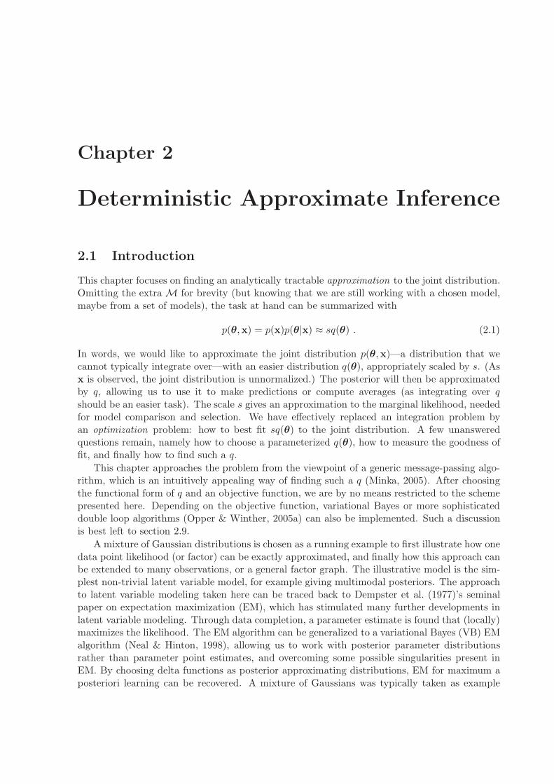
2.3 A simple mixture of Gaussians

As a simple illustration of different divergence measures, consider a one-dimensional Gaussianmixture with unknown means, so that θ ≡ µ,

p(xn|µ) =J∑

j=1

πjN (xn|µj , λ−1j ) , (2.9)

where

N (xn|µj , λ−1j ) =

(λj

2π

)1/2e−

12λj(xn−µj)

2=

1

ZN (λj)e−

12λj(xn−µj)

2. (2.10)

In the above mixture of J Gaussians, we let each precision (inverse variance) λj, as well asthe mixing weights π, be known. The unknown parameters θ are therefore the set of meansµ = {µj}Jj=1. Let the prior on the means be conjugate and hence Gaussian,

p(µ) =J∏

j=1

p(µj) =J∏

j=1

N (µj |m0j , v−10j ) . (2.11)

For q we choose a product of Gaussians, one each to model the mean of a component in themixture,

q(µ) =

J∏

j=1

q(µj) =

J∏

j=1

N (µj |mj, v−1j ) . (2.12)

In many cases our choice of approximating distribution will be restricted by the model. Forone observation (let it be xn, for instance) our task is to match sq(µ) ≈ p(xn|µ)p(µ) We candirectly minimize both KL divergences, but need to resort to an iterative method to minimizeother α-divergences. As the cases of α = 1 and α = 0 ultimately expand respectively intoexpectation propagation and variational Bayes, the sections that follow here are appropriatelyheaded.

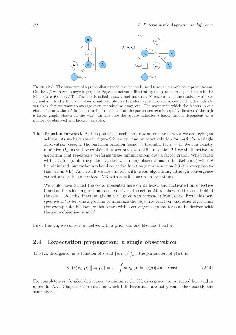
As an interlude, it is worthwhile to visualize the joint distribution in a graphical represen-tation, given in figure 2.3. The following two equations are illustrated, where the first gives theparameter dependencies, while the second gives a chosen factorization,

p(x, z,µ) =

N∏

n=1

p(xn|µ, z)p(z)p(µ) =

N∏

n=1

J∏

j=1

N(xn|µj, λ

−1j

)znj × πznj

j ×N(µj |m0j , v

−10j

)

=

N∏

n=1

fn(µ, zn)× f0(µ) . (2.13)

Each of the factors in the factor graph will ultimately be approximated.

30 2. Deterministic Approximate Inference

N

zn

π

µ λxn

m0, v0

N

π

f0(µ) µ λ

xn

zn

fn(µ, zn)

m0, v0

Figure 2.3: The structure of a probabilistic model can be made lucid through a graphical representation.On the left we have an acyclic graph or Bayesian network, illustrating the parameter dependencies in thejoint p(x, z,θ) in (2.13). The box is called a plate, and indicates N replicates of the random variablesxn and zn. Nodes that are coloured indicate observed random variables, and uncoloured nodes indicatevariables that we want to average over, marginalize away, etc. The manner in which the factors in ourchosen factorization of the joint distribution depend on the parameters can be equally illustrated througha factor graph, shown on the right. In this case the square indicates a factor that is dependent on anumber of observed and hidden variables.

The direction forward. At this point it is useful to draw an outline of what we are trying toachieve. As we have seen in figure 2.2, we can find an exact solution for sq(θ) for a ‘singleobservation’ case, as the partition function (scale) is tractable for α = 1. We can exactlyminimize Dα, as will be explained in sections 2.4 to 2.6. In section 2.7 we shall motive analgorithm that repeatedly performs these minimizations over a factor graph. When facedwith a factor graph, the global Dα (i.e. with many observations in the likelihood) will notbe minimized, but rather a related objective function given in section 2.9 (the exception tothis rule is VB). As a result we are still left with useful algorithms, although convergencecannot always be guaranteed (VB with α = 0 is again an exception).

We could have turned the order presented here on its head, and motivated an objectivefunction, for which algorithms can be derived. In section 2.9 we show solid reason behindthe α = 1 objective function, giving the expectation consistent framework. From this per-spective EP is but one algorithm to minimize the objective function, and other algorithms(for example double loop, which comes with a convergence guarantee) can be derived withthe same objective in mind.

First, though, we concern ourselves with a prior and one likelihood factor.

2.4 Expectation propagation: a single observation

The KL divergence, as a function of s and {mj , vj}Jj=1, the parameters of q(µ), is

KL(p(xn,µ)

∥∥ sq(µ)

)= s−

∫

p(xn,µ) ln[sq(µ)] dµ + const . (2.14)

For completeness, detailed derivations to minimize the KL divergence are presented here and inappendix A.2. Chapter 3’s results, for which full derivations are not given, follow exactly thesame style.

2.4. Expectation propagation: a single observation 31

2.4.1 The scale

Taking derivatives of (2.14) with respect to s, and equating to zero, gives s =∫p(xn,µ) dµ.

From observing one example, we can directly write down the marginal likelihood as a functionof the prior parameter values,

s = s(m0, v0) =

J∑

j=1

πj

∫

p(xn|µj)p(µj) dµj =

J∑

j=1

πjN (xn|m0j , λ−10j + v−1

0j ) . (2.15)

2.4.2 Parameter updates for the components

The parameter updates of each approximate distributions q(µj) will take the form of a weightedsum of the prior and component-posterior moments, which has an intuitively pleasing expla-nation: The moments of q(µj) are calculated by determining the probability of component jgenerating xn, multiplied by the moment of including xn into component j, plus the probabil-ity of component j not generating xn, multiplied by the prior moment of component j. Themoment-matching equations can be determined with

∂KL(p(xn,µ)

∥∥ sq(µ)

)/∂mj = 0 , (2.16)

which we derive in appendix A.2. In this vein, define the responsibilities as

rnj =πj

∫p(µj)p(xn|µj) dµj

∑

k πk

∫p(µk)p(xn|µk) dµk

=πjN (xn|m0j , λ

−1j + v−1

0j )∑

k πkN (xn|m0k, λ−1k + v−1

0k ), (2.17)

so that the mean of the approximation is therefore a responsibility-weighted sum of the priorand component-posterior means, or a weighted sum of moments,

mj = (1− rnj)

∫

µjp(µj) dµj + rnj

∫

µjp(µj|xn) dµj

= (1− rnj)〈µj〉+ rnj〈µj |xn〉 . (2.18)

Exactly the same can be done for the precision parameters. Differentiating the KL divergencewith respect to vj gives (following the same type of arrangement of terms as we have done forthe means),

1

vj= (1− rnj)

∫

(µj −mj)2p(µj) dµj + rnj

∫

(µj −mj)2p(µj|xn) dµj . (2.19)

By substituting the value ofmj , we arrive at the second of the elegant weighted moment-matchingequations,

1

vj= (1− rnj)〈µ2

j 〉+ rnj〈µ2j |xn〉 −m2

j . (2.20)

The following expectations are used in the update to get an approximation q(µj) = N (µj|mj , v−1j ),

〈µj〉 = m0j (2.21)

〈µj|xn〉 =λjxn + v0jm0j

λj + v0j(2.22)

〈µ2j〉 = var(µj) + 〈µj〉2 =

1

v0j+m2

0j (2.23)

〈µ2j |xn〉 = var(µj |xn) + 〈µj|xn〉2 =

1

λj + v0j+(λ0jxn + v0jm0j

λj + v0j

)2. (2.24)

32 2. Deterministic Approximate Inference

2.5 Variational Bayes: a single observation

For VB we introduce latent allocation variables, so that the sum in the joint distribution becomesa product. Let zn ∈ {0, 1}J be a binary latent variable, with

∑Jj=1 znj = 1, indicating which

component in the mixture generated the data point. Therefore

p(xn,µ, zn) = p(xn|µ, zn)p(zn)p(µ) =J∏

j=1

p(xn|µj)znj ×

J∏

j=1

πznj

j × p(µ) . (2.25)

For the α-divergence minimization in section 2.6, this method of data completion is also used.We could equally have done it for EP as well: the result will be exactly the same, as substitutingα = 1 in section 2.6’s fixed point scheme clearly shows.

The joint distribution will be approximated with sq(µ)q(zn), where q(zn) is multinomial,

q(zn) =

J∏

j=1

γznj

nj (2.26)

with γnj ≥ 0 and∑

j γnj = 1.

A mean field approximation to our simple posterior can be found by ‘reversing the KLdivergence’ to its ‘exclusive’ form. Again, we write the KL divergence as a function of s and theparameters of q(µ) and q(zn):

KL(sq(µ)q(zn)

∥∥ p(xn,µ, zn)

)=

∫∑

zn

sq(µ)q(zn) lnsq(µ)q(zn)

p(xn,µ, zn)dµ− s+ const

= s ln s+ s〈ln q(µ)〉+ s〈ln q(zn)〉− s〈ln p(xn,µ, zn)〉 − s+ const . (2.27)

2.5.1 Parameter updates

To optimize over distributions q(µ) and q(zn), take the functional derivative of the KL diver-gence (2.27) with respect to q(µ) and q(zn), in each case equating to zero and solving. It isshown below that we arrive at an iterative optimization procedure, which is a single-observationimplementation of VBEM. In essence we are doing an iterative coordinate descent procedure overfunctions (distributions) q, which will converge to a local minimum as each of the subproblemsis convex. The following E- and M-steps are repeated until convergence.

E-step. For the expectation step, we keep q(µ) fixed. Zeroing the functional derivative of (2.27)with respect to q(zn) gives

q(zn) ∝ exp{∫

q(µ) ln p(xn,µ, zn) dµ}

. (2.28)

Because we can rewrite ln p(xn, zn,µ) as ln p(xn, zn|µ) + ln p(µ), the above equation canbe simplified as q(zn) ∝ exp{

∫q(µ) ln p(xn, zn|µ) dµ}. If mj and vj are the present

parameters of q(µj) (we can start with a guess, e.g. set to the prior), then

∫

q(µ) ln p(xn, zn|µ)dµ =J∑

j=1

znj

∫ [

lnπj− lnZN

(λj)−λj

2(xn−µj)

2]

q(µj)dµj , (2.29)

2.5. Variational Bayes: a single observation 33

and hence the responsibilities, characterizing q(zn), will be

γnj =πj

√λj exp{−λj

2 (v−1j + (mj − xn)2)}

∑

k πk

√λk exp{−λk

2 (v−1k + (mk − xn)2)}

. (2.30)

M-step. For the maximization step, the derivation of the E-step is repeated, only with q(µ)and q(zn) swapping roles,

q(µ) ∝ exp{∑

zn

q(zn) ln p(xn,µ, zn)}

. (2.31)

To update the parameters, note that

∑

zn

q(zn) ln[p(xn, zn|µ)p(µ)

]= −

∑

zn

J∏

i=1

γznini

J∑

j=1

znjλj

2(xn − µj)

2 −J∑

j=1

v0j

2(µj −m0j)

2 + const

= −J∑

j=1

1

2(v0j + γnjλj)

(

µj −v0jm0j + γnjλjxn

v0j + γnjλj

)2+ const .

(2.32)

This is in the form of an unnormalized q(µ), and hence the parameter updates are

vj = v0j + γnjλj (2.33)

mj =v0jm0j + γnjλjxn

v0j + γnjλj. (2.34)

2.5.2 The scale

After optimizing for the parameters of q, we find the matching scale s by taking the partialderivative of (2.27) with respect to s and equating it to zero. In this case log scale ln s alsocorresponds to the negative variational free energy from mean field methods or statistical physics.The approximation to the log marginal likelihood is therefore

ln s = 〈ln p(xn,µ, zn)〉 − 〈ln q(µ)〉 − 〈ln q(zn)〉 . (2.35)

This we determine from the following equations:

〈ln p(xn,µ, zn)〉 =⟨ J∑

j=1

znj ln p(xn|µj)⟩

+⟨ J∑

j=1

znj lnπj

⟩

+⟨ J∑

j=1

ln p(µj)⟩

=

J∑

j=1

γnj

[

− lnZN (λj)−λj

2

( 1

vj+ (mj − xn)2

)]

+

J∑

j=1

γnj lnπj +

J∑

j=1

[

− lnZN

(v0j)−v0j

2

( 1

vj+ (mj −m0j)

2)]

(2.36)

〈ln q(µ)〉 =J∑

j=1

〈ln q(µj)〉 = −J∑

j=1

lnZN

(vj)−J

2(2.37)

〈ln q(zn)〉 =

J∑

j=1

γnj ln γnj . (2.38)

34 2. Deterministic Approximate Inference

2.6 α-divergence: a single observation

More generally we seek a sq(θ) that minimizes Dα(p(x,θ) ‖ sq(θ)), and this section presents areview on how an α-divergence can be minimized by repeatedly minimizing a KL divergence.The review is followed by a new contribution in section 2.6.1 on minimizing Dα for a simplemixtures problem. This contribution is reworked in section 3.5 to provide a key step for a newfactor graph algorithm for full-blown mixture of Gaussians.

We let sq(θ) be a member of some scaled exponential family F , for example the family ofscaled Gaussians. The following theorem provides a key to finding the minimum:

Theorem 2. (Minka, 2005). If α 6= 0 then sq(θ) is a stationary point of

Dα(p(x,θ) ‖ sq(θ)) (2.39)

if and only if sq(θ) is a stationary point of

arg minsq(θ)∈F

KL

(

p(x,θ)α[sq(θ)]1−α∥∥ sq(θ)

)

. (2.40)

Proof. We show that the derivatives match at sq(θ) = s∗q∗(θ), i.e.

∂KL(p(x,θ)α[s∗q∗(θ)]1−α ‖ sq(θ))

∂[sq(θ)]

∣∣∣∣∣sq(θ)=s∗q∗(θ)

∝ ∂Dα(p(x,θ) ‖ sq(θ))

∂[sq(θ)]

∣∣∣∣∣sq(θ)=s∗q∗(θ)

, (2.41)

which we show by taking functional derivatives with respect to sq(θ), and substituting sq(θ) =s∗q∗(θ),

∂Dα(p(x,θ) ‖ sq(θ))

∂[sq(θ)]=

1

α

[

1−∫ (p(x,θ)

sq(θ)

)αdθ]

(2.42)

∂KL(p(x,θ)α[s∗q∗(θ)]1−α ‖ sq(θ))

∂[sq(θ)]= 1−

∫p(x,θ)α[s∗q∗(θ)]1−α

sq(θ)dθ . (2.43)

Consequently when s∗q∗(θ) is a stationary point of Dα (derivative = 0), it is also a stationarypoint of KL, as its derivative must also be zero.

The proof given above is equivalent to, but marginally different from that given by Minka(2005), where derivatives with respect to the parameters of q were used. To find such a stationarypoint, we turn to a fixed point scheme. Define

f(s∗q∗(θ)) = arg minsq(θ)∈F

KL

(

p(x,θ)α[s∗q∗(θ)]1−α∥∥ sq(θ)

)

(2.44)

so that we need to solve forf(s∗q∗(θ)) = s∗q∗(θ) . (2.45)

This can be done with a typical fixed point algorithm to give

s(t+1)q(t+1)(θ) = f(s(t)q(t)(θ)) (2.46)

which we repeat until convergence. Minka (2005) suggests the addition of damping to the fixedpoint iterations, as the scheme is heuristic and not guaranteed to converge, but it is oftensuccessful with enough damping. We have the following fixed point scheme, which is illustratedin figure 2.4. We start with a guess of an initial s(0)q(0)(θ), where q(0)(θ) is normalized, andtypically take s(0) = 1. Starting with t= 0, the following two steps are iterated until convergence.

2.6. α-divergence: a single observation 35

F

p(x, θ)α[s(t)q(t)(θ)]1−α

s(t)q(t)(θ)s(t′)q(t′)(θ)

p(x, θ)

min Dα

(p(x, θ)‖sq(θ)

)

sq(θ)

min KL(p(x, θ)α[s(t)q(t)(θ)]1−α ‖ s(t′)q(t′)(θ)

)

s(t+1)q(t+1)(θ) = [s(t)q(t)(θ)]ǫ[s(t′)q(t′)(θ)]1−ǫ

p(x, θ)α[s(t+1)q(t+1)(θ)]1−α

F

Figure 2.4: An α-divergence can be minimized by iteratively minimizing a KL divergence. Our aim,shown on the right, is to find an element sq(θ) ∈ F that is closest to p(x,θ) (which we assume is notin a chosen scaled exponential family F) with respect to divergence Dα. This is solved through theiterative method on the left. For some s(t)q(t)(θ) ∈ F , a function p(x,θ)α[s(t)q(t)(θ)]1−α that is not in Fis created, and now an element in F closest to it with respect to the KL divergence is found. After somepossible damping, this process is repeated.

Step 1. We find s(t′)q(t′)(θ),

s(t′)q(t′)(θ) = arg minsq(θ)

KL(p(x,θ)α[s(t)q(t)(θ)]1−α

∥∥ sq(θ)

), (2.47)

by first computing the new scale

s(t′) =

∫

p(x,θ)α[s(t)q(t)(θ)]1−αdθ = s1−α(t)

∫

p(x,θ)αq(t)(θ)1−αdθ . (2.48)

Now use p(x,θ)αq(t)(θ)1−α as the ‘joint’ distribution, and find a normalized q(t′)(θ) thatminimizes KL

(p(x,θ)αq(t)(θ)1−α

∥∥ q(t′)(θ)

)by matching moments, as we have done in

section 2.4. (The scale is excluded for simplicity, as we have already found it.)

Step 2. We now have s(t′)q(t′)(θ). If we had α = 1, this would have been perfectly sufficient.We damp it with

s(t+1)q(t+1)(θ) = [s(t)q(t)(θ)]ǫ[s(t′)q(t′)(θ)]1−ǫ . (2.49)

After implementing the above damping equation, we rearrange the product to keep q(t+1)

as a normalized distribution. Therefore set

q(t+1)(θ) = Z−1q(t)(θ)ǫq(t′)(θ)1−ǫ (2.50)

with Z =

∫

q(t)(θ)ǫq(t′)(θ)1−ǫdθ , (2.51)

and then set s(t+1) = sǫ(t)s

1−ǫ(t′) Z . (2.52)

This heuristic scheme is iterated until convergence, and the final s(t+1) and q(t+1) are taken asminimizers of α-divergence. Convergence of the heuristic scheme depends on the amount ofdamping ǫ, and α.

2.6.1 Fixed point iterations

The fixed point scheme involves the ‘prior’ p(µ)αq(t)(µ)1−α, for which we define the followingshorthand parameters:

vi = αv0i + (1− α)vi(t) (2.53)

36 2. Deterministic Approximate Inference

mi =αv0im0i + (1− α)vi(t)mi(t)

αv0i + (1− α)vi(t). (2.54)

To run the fixed point scheme, start with an initial s(0)q(0)(zn)q(0)(µ), where s(0) is set to one,and the parameters γnj of q(0)(zn) possibly set to 1/J . q(0)(µ) can be set to the prior. Startingwith t = 0, the following steps are repeated until convergence, or until some maximum numberof iterations is reached.

Step 1. Determine the scale, which follows from appendix A.4.1 as

s(t′) =

∫∑

zn

p(xn,µ, zn)α[s(t)q(t)(zn)q(t)(µ)]1−αdµ

= s1−α(t)

J∏

i=1

ZN

(vi)

ZN

(v0i)αZN(vi(t))1−α

exp{

− 1

2

αv0i(1− α)vi(t)

vi

[m0i −mi(t)

]2}

× α−1/2J∑

k=1

παk γ

1−αnk(t)ZN

(λk)1−αN

(

xn

∣∣∣ mk,

1

αλk+

1

vk

)

. (2.55)

Following the scale, we find a normalized distribution q(t′)(zn)q(t′)(µ) that will minimizethe KL divergence to p(xn,µ, zn)α[q(t)(zn)q(t)(µ)]1−α. We have already solved for the scaleand only need to match moments, for which the following expectations are used:

〈µj〉 = mj (2.56)

〈µj|xn〉 =vjmj + αλjxn

vj + αλj(2.57)

〈µ2j 〉 =

1

vj+ 〈µj〉2 (2.58)

〈µ2j |xn〉 =

1

vj + αλj+ 〈µj|xn〉2 . (2.59)

Define

rnj =πα

j γ1−αnj(t)N (xn | mj , (αλj)

−1 + v−1j )

∑

k παk γ

1−αnk(t)N (xn | mk, (αλk)−1 + v−1

k ), (2.60)

so that the updates again involve matching weighed moments,

mj(t′) = (1− rnj)〈µj〉+ rnj〈µj|xn〉 (2.61)

1

vj(t′)= (1− rnj)〈µ2

j 〉+ rnj〈µ2j |xn〉 −m2

j(t′) (2.62)

γnj(t′) = rnj . (2.63)

The only difference from the standard EP update is that an exponentiated likelihood wasused; the mean and precision follows the same type of derivation as before. The derivationfor γnj(t′) follows in appendix A.5.

Step 2. We have s(t′)q(t′)(zn)q(t′)(µ), and for the damping step need to do a derivation similarto the first step to find a normalized q(t+1). Define the mean and precision of the new(unscaled) Gaussian q(t)(µ)ǫq(t′)(µ)1−ǫ as

vj(t+1) = ǫvj(t) + (1− ǫ)vj(t′) (2.64)

2.7. Minimizing over a factor graph 37

mj(t+1) =ǫvj(t)mj(t) + (1− ǫ)vj(t′)mj(t′)

ǫvj(t) + (1− ǫ)vj(t′)(2.65)

for each component j. Then damping gives

q(t)(µ)ǫq(t′)(µ)1−ǫ =J∏

j=1

1

ZN

(vj(t))ǫ1

ZN

(vj(t′))1−ǫexp

{

− 1

2

ǫvj(t)(1− ǫ)vj(t′)

vj(t+1)(mj(t) −mj(t′))

2}

× exp{

− 1

2vj(t+1)(µj −mj(t+1))

2}

(2.66)

q(t)(zn)ǫq(t′)(zn)1−ǫ =

J∏

j=1

[γǫnj(t)γ

1−ǫnj(t′)]

znj . (2.67)

We would like to keep q(t+1) as a normalized distribution, and hence set

q(t+1)(µ) = Z−11 q(t)(µ)ǫq(t′)(µ)1−ǫ . (2.68)

The means and precisions will not change, but we have to keep track of the scale that wehave to divide with to ensure that q(t+1)(µ) remains normalized. That scale is

Z1 =

J∏

j=1

ZN

(vj(t+1))

ZN

(vj(t))ǫZN(vj(t′))1−ǫ

exp{

− 1

2

ǫvj(t)(1− ǫ)vj(t′)

vj(t+1)(mj(t) −mj(t′))

2}

. (2.69)

Similarly, set the parameters of q(t+1)(zn) as

γnj(t+1) = Z−12 γǫ

nj(t)γ1−ǫnj(t′) , (2.70)

where the multinomial was normalized with

Z2 =J∑

k=1

γǫnk(t)γ

1−ǫnk(t′)

. (2.71)

Finally adjust the scale, remembering that we had to divide by Z1 and Z2 to keep qnormalized. Add the appropriate log normalizers to get the updated log marginal likelihoodestimate,

ln s(t+1) = ǫ ln s(t) + (1− ǫ) ln s(t′) + lnZ1 + lnZ2 . (2.72)

2.7 Minimizing over a factor graph

So far we have a general method of approximating a joint distribution, consisting of a prior andone observation, with a simpler distribution. On a factor graph, as in figure 2.3, this correspondsto approximating a ‘prior’ and ‘data’ factor. The approximation scheme can be extended overa full factor graph or full joint distribution. In this section we want to find a scaled distributionsq(θ) to match a full joint,

sq(θ) ≈ p(x,θ) =N∏

n=1

p(xn|θ)p(θ) =N∏

n=0

fn(θ) , (2.73)

and we hope to again find this by minimizing Dα. We have written the joint distribution as aproduct of factors, and the way that we choose the factorization need not be unique. In this

38 2. Deterministic Approximate Inference

chapter a single data likelihood is chosen as a factor. In the full mixture of Gaussians thatfollows in chapter 3, we could equally have split the data likelihood into a mixture weight factorand a factor modeling the component parameters.

Let sq(θ) be a member of a scaled exponential family F . Our choice is motivated as only afinite number of moments need to be propagated through the factor graph. The family is closedunder multiplication, as the product of any number of distributions in F is also in F . (Whenspeaking about sq(θ), we have previously restricted F to normalizable exponential functions,for example in the iterative optimization scheme of section 2.6. Here we extend the exponentialsto include factor approximations, which aren’t necessarily normalizable, as well.) Each factorwill be approximated by a member of F ,

fn(θ) = sn exp{∑

m

φm(θ)ηnm

}

= sn exp{

η⊤n φ(θ)

}

= snf′n(θ) , (2.74)

where η is some natural parameter vector, and φ(θ) is the vector of sufficient statistics or featuresof the distribution, e.g. φ(θ) = (θ2, θ, 1) for a one dimensional Gaussian, and η = (−1

2v, vm, c).The factor definition has been made deliberately loosely; ‘1’ has been added as a feature, to allowa choice for extra constant terms c in the exponential. This addition is possible as the exponentialis again rescaled by some constant sn, which we are free to choose. In the continuation of themixtures example, we choose c = −1

2vm2, for example, so that η⊤φ(θ) factorizes over θ with

the usual −v2(θ −m)2.

The factor approximations need not be normalizable; however, their product must be, andequal to sq(θ) ∈ F ,

sq(θ) =

N∏

n=0

fn(θ) . (2.75)

The following section describes how the above approximation can be found by considering singlefactors at a time.

2.7.1 A generic message passing algorithm

Assume that we have an approximation for all factors, except for a factor n, and that we wantto include fn in the approximation. Now define two distributions, the joint without factor fn’sinclusion,

p\n(x,θ) =∏

i6=n

fi(θ) , (2.76)

and the approximation excluding approximate factor fn,

s\nq\n(θ) = sq(θ)/fn(θ) =∏

i6=n

fi(θ) . (2.77)

In ideal circumstances factor fn should minimize

Dα

(p\n(x,θ)fn(θ)

∥∥ s\nq\n(θ)fn(θ)

), (2.78)

which gives rise to an intractable minimization problem. A tractable road forward exists, andthat is to assume that the approximation made to the rest of the factor graph is a good one, sothat

p\n(x,θ) ≈ s\nq\n(θ) . (2.79)

2.7. Minimizing over a factor graph 39

Algorithm 1 Generic message passing algorithm

1: initialize: fn(θ) for all n.2: repeat3: pick a factor n.4: compute s\nq\n(θ).5: update the factor approximation fn(θ) by getting the new approximation to the joint

snewq(θ)new with equation (2.81), and solve for the updated term contribution fn with(2.83).

6: until all fn(θ) converge.

It may be helpful to interpret this assumption in the following way (specific to the examples inthis chapter, although the method is much more general): If single data likelihoods are taken asfactors, this simply means that all the data that we have already included in the approximationcan be summarized in some form of scaled prior distribution s\nq\n(θ), which needs to bemultiplied by the data term factor fn (or likelihood p(xn|θ)), to get a new approximation to thejoint distribution.

The problem simplifies to that of finding a fn that minimizes

Dα

(s\nq\n(θ)fn(θ)

∥∥ s\nq\n(θ)fn(θ)

). (2.80)

In light of the methods presented in sections 2.4 to 2.6, where some sq(θ) is matched to a priortimes a likelihood, we find fn by finding a new scaled approximation snewq(θ)new, with

snewq(θ)new = arg minsq(θ)

Dα

(s\nq\n(θ)fn(θ)

∥∥ sq(θ)

), (2.81)

and then using snewq(θ)new and s\nq\n(θ) to find fn(θ). This is purely a matter of division, aswe are using the exponential family of distributions. We have

s\nq\n(θ)fn(θ) = snewq(θ)new , (2.82)

and hence

fn(θ) =snew

s\nq(θ)new

q\n(θ). (2.83)

The resulting message passing algorithm is summarized in algorithm 1.

2.7.2 Minimizing the mixtures example over a factor graph

For our practical implementation it is not necessary to determine s\n when we want to updatethe scale contribution sn, as

Sq(θ)new = arg mins′q(θ)

Dα

(q\n(θ)fn(θ)

∥∥ s′q(θ)

)(2.84)

gives the same minimum as equation (2.81), with snew = Ss\n, and equation (2.83) thereforegives fn(θ) = Sq(θ)new/q\n(θ). This slightly simplified restatement will be used in the mini-mization routine that follows.

We choose term definitions fn, for Gaussian components with unknown means, as

fn = sn

J∏

j=1

e−12vnj(µj−mnj )2 . (2.85)

The message passing algorithm is:

40 2. Deterministic Approximate Inference

• Start by initializing, for n = 1, . . . ,N ,

sn = 1, mnj = 0, and vnj = 0 , (2.86)

so that all the factor approximations are one. Initialize the prior as

s0 =J∏

j=1

1

ZN (v0j)=

J∏

j=1

(v0j/2π)1/2, m0j = m0j , and v0j = v0j . (2.87)

• Repeat until all fn converge:

1. Pick a factor n. This can be done by looping over different random permutations of1, . . . , N .

2. Compute q\n(µ) (for reasons stated above we need not concern ourselves with s\n).We take the convention of identifying the parameters of q\n(µ) with a subscripto for ‘old’, where ‘old’ refers to our approximation before including term n. Thisconvention is also followed because here q\n(µ) takes the role of a prior, allowing astraight-forward implementation of the optimization routines of sections 2.4 to 2.6.Recovering the old distribution—also referred to as the cavity distribution—followsfrom reversing equations (2.91) and (2.92),

voj = vj − vnj (2.88)

moj =vjmj − vnjmnj

voj. (2.89)

If a non-normalizable distribution is recovered, the update for factor fn can beskipped, and we continue again from step 1.

3. Similar to sections 2.4 to 2.6, let S, mj and vj be the parameters of q(µ)new thatminimizes equation (2.84). After finding the new approximation, we have to set thefactor contribution. After a rearrangement so that a single exponential depends onµj, we get

fn = Sq(µ)new

q\n(µ)

= S

J∏

j=1

ZN (voj)

ZN

(vj)exp

{

+1

2

vjvoj

vj − voj(mj −moj)

2}

· · ·J∏

j=1

exp{

− 1

2(vj − voj)

[µj −

vjmj − vojmoj

vj − voj

]2}

. (2.90)

According to our term definition (2.85), we get the substitution for vnj and mnj forj = 1, . . . , J , and for the change of scale sn, as

vnj = vj − voj (2.91)

mnj =vjmj − vojmoj

vnj(2.92)

sn = S

J∏

j=1

ZN (voj)

ZN

(vj)exp

{

+1

2

vjvoj

vj − voj(mj −moj)

2}

. (2.93)

2.8. Model pruning 41

• Finally the approximation to the evidence p(x) is determined with

p(x) ≈∫ N∏

n=0

fn(µ) dµ =( N∏

n=0

sn

) J∏

j=1

e12[vjm2

j−PN

n=0 vnjm2nj ]ZN (vj) . (2.94)

Starting with another prior contribution

We need not start by initializing the prior contribution s0, m0j and v0j ∀j to the prior hyper-parameter values; sometimes we may wish to break symmetry so that the iterative algorithmconverges to one solution rather than another. This may be necessary when the prior is sym-metric around zero, causing the responsibilities to always remain equal, stifling any progress. Atypical example may be when the posterior has more than one equivalent mode (as often hap-pens in mixtures models, which are invariant with respect to permutations of the componentlabeling). When the modes are well separated we may want to approximate one of them, i.e.break symmetry and not find a solution with small mass balanced between them.

To break symmetry we start with the ‘wrong’ prior, and can always go back after the firstloop over factors to correct the prior contributions to the correct prior hyperparameter values.(In practice, if m0j = 0 ∀j, for example, we may start with m0j = ǫj where ǫj represents someadded symmetry-breaking noise.)

If we did choose to start with the wrong prior contributions, the prior is treated like anyother factor. The hyperparameter values need not to be set in any optimization routine, as theyare prespecified and fixed. We find q(µ)new with

vj = voj + v0j and mj = (vojmoj + v0jm0j)/(voj + v0j) , (2.95)

and update the prior contribution to the correct hyperparameters,

s0 =

J∏

j=1

1

ZN

(v0j), m0j = m0j, and v0j = v0j . (2.96)

2.8 Model pruning

The aim of this discussion is to look at the behavior of VB and EP on very simple examples.This will mostly be in light of chapter 3, for when we understand the behavior of the algorithmsunder different settings, we can intuitively explain certain higher-dimensional phenomena.

A problem that may arise when a free energy is minimized in variational Bayes (α = 0), isthat the degrees of freedom in the parameter space may be pruned, perhaps even inappropriately(MacKay, 2001). A mixture model, as is the example in this chapter, may self-prune. If we addmore components to the model we believe in, the extra components and parameters may notbe used at all. This is contrary to our expectation, where we expect all the parameters to beincluded in the posterior, maybe with big error bars on them.

Let’s first reflect back on a well-behaved example. For figure 2.1(a) we had J = 2 components,and found an approximation sq(µ) that gave equal weight to each mixture component. In theapproximation q(µ1) and q(µ2) are equal, and γn1 = γn2 = 1

2 (with one observation, N = 1).This is what we would expect, as we have no motivation to prefer one component over the other.(All precisions were set to λj = 1, the mixing weights were fixed at πj = 1

2 , and v0j = 0.1 andm0j = 0 were taken as prior parameter values.)

A typical example of unwanted pruning is found in figure 2.5(a), which is similar to an ex-ample encountered before in figure 2.1(a), but with a broader prior value v0j = 0.01. Apart from

42 2. Deterministic Approximate Inference

µ2

µ1

(a) A possible approximate solution for the fixedpoint equation (2.97), showing one componentbeing pruned.

0 0.2 0.4 0.6 0.8 10

0.2

0.4

0.6

0.8

1

γ

(b) Possible solutions to equation (2.97), at theintersections of the functions γ and g(γ) = 1/(1+exp{ 1

2( 1

v1− 1

v2)}). There are in fact five intersec-

tions, at γ ≈ 0, 0.38, 0.5, 0.62 and 1.

Figure 2.5: Local solutions with a broader prior v0j = 0.01. With J = 2 components, the other prior

parameter values we set to πj = 12 , m0j = 0 and λj = 1.

γn1 = 0.5, there are four other local maxima in the free energy, − ln s, with γn1 ≈ 0, 0.38, 0.62and 1. With γn1 ≈ 1, and its converse, one of the mixture components is lost, with its approxi-mation effectively being equal to the prior. (The values of γnj are not strictly at zero and one,but asymptotically close as v0j shrinks to give a broader prior.) There would be no reason forus to favor any model, as the single xn = 0 could have been generated by the first or secondcomponent, but yet that is what the local minima in the free energy would lead us to believe.

As we have only one data point and two components, let γ ≡ γn1. From equations (2.30)and (2.33) we have

γ =1

1 + exp{

12 ( 1

v1− 1

v2)} , where v1 = v01 + γλ1 and v2 = v02 + (1− γ)λ2 , (2.97)

with the values of λj fixed at 1. To solve for the extrema, we need to find a value of γ such thatequation (2.97) holds. With function g(γ) = 1/(1 + exp{1

2 ( 1v1− 1

v2)}), this can be solved with a

fixed point equation

γnew ← g(γ) , (2.98)

which is merely the VBEM algorithm in another form. Figure 2.5(b) shows a plot of γ and g(γ)with a broader prior v0j = 0.01. The free energy minima occur at the intersection of these twofunctions.

If we narrow the prior and make v0j bigger, the symmetry-breaking solutions are lost. Figure2.6 illustrates this phenomena. There is a critical value of v0j ≈ 0.97 that separates our notionof symmetry-breaking and symmetry preserving priors in this example, where bigger precisions(smaller variances) preserve the symmetry. This gives some bifurcation, as there is a very suddensplit between many possible solutions and only one.

The relevance of this discussion finds form in section 3.7, where VB is run over a factorgraph. As factors (or data points) are included one at a time, this differs from conventional VB,where all data points are treated together in an EM algorithm. MacKay (2001) illustrates thatunwanted model pruning becomes less of a problem with more data present in standard VB.By including one data point at a time, or optimizing on a factor by factor basis, it has beenfound in practice (section 3.7) that components can be lost on the inclusion of the first data

2.9. The objective function 43

0 0.2 0.4 0.6 0.8 10

0.2

0.4

0.6

0.8

1

γ

g(γ) with v0j

= 0.001

g(γ) with v0j

= 0.02

g(γ) with v0j

= 0.097

g(γ) with v0j

= 0.4

γ

Increasing v0j

Figure 2.6: If the prior from figure 2.5 is narrowed, the symmetry-breaking solutions are lost, so thatthe only solution to the fixed point equation (2.97) would be a spherical Gaussian centered at zero. Thefigure also illustrates a critical value v0j ≈ 0.97 where a bifurcation occurs, as we see a very sudden splitbetween many possible solutions (intersections) and only one.

point to a broad prior. This puts us in a situation where some components are almost zero-weighted after the addition of the first factor, and the inclusion of subsequent factors cannotrecover these components. As we will see next, EP doesn’t suffer from this drawback, and thesolution adopted in section 3.7 is to run one or two EP loops over all factors to give a sensibleinitialization of approximate factors before the VB loops are run.

Model pruning and expectation propagation

An approximation scheme like EP will not suffer under the same component-pruning behaviour,as the parameter updates take a on a very different form.

• For VB we solved using the EM fixed point equations, and iterated an expectation andmaximization step. The E-step determined responsibilities that depend on the presentparameter settings and not the prior. The M-step then depended on the responsibilitiesand prior. Equations (2.30), (2.33) and (2.34) give an example of these dependencies.

• EP relied on two steps as well, but they are not iterated. The first was a responsibilityupdate that depends on the prior and not any present parameter values. It was followed bya moment matching step that depends on the responsibility-weighed prior and component-posterior moments. Equations (2.17), (2.18) and (2.20) can be taken as an example.

2.9 The objective function

Under a set of constrains, the generic message passing algorithm would attempt to find thelargest scale s for a given normalized distribution q(θ) and an associated joint distribution

44 2. Deterministic Approximate Inference

p(x,θ). In other words, given a factorized approximation, we can determine the scale, andtherefore need to maximize some objective function over the approximate factors such that thescale is as big as possible. This was clearly seen in the case of variational Bayes, for example,where s was always a lower bound to the true marginal likelihood p(x), and we had to adjust theapproximating distribution so that the scale (as a function of the approximating distribution)could be as big as possible.

We will show here, following (Minka, 2005), that the generic message passing iterations fromalgorithm 1 always have a fixed point when the approximations are in the exponential family.This does not mean that the fixed point will necessarily be found, even though its objectivefunction is well defined. It is a single loop algorithm, and longer double-loop algorithms, whichcome with a convergence guarantee, can be created to minimize the same objective functionOpper & Winther (2005a).

The scale that will be computed by message-passing can be written as

s =

∫

sq(θ) dθ =

∫ N∏

n=0

fn(θ) dθ =( N∏

n=0

sn

)∫ N∏

n=0

f ′n(θ) dθ =( N∏

n=0

sn

)∫

q′(θ) dθ (2.99)

where we have defined the shortcut q′(θ) =∏

n f′n(θ). The final approximation has the form

q(θ) ∝ q′(θ) =

N∏

n=0

f ′n(θ) =

N∏

n=0

exp{

η⊤n φ(θ)

}

= exp{ N∑

n=0

η⊤n φ(θ)

}

(2.100)

for some η ≡ {ηn}Nn=0. Each leave-one-out (cavity) distribution has the form

q\n(θ) ∝∏

i6=n

f ′i(θ) = exp{∑

i6=n

η⊤i φ(θ)

}

. (2.101)

The following two sections treat α 6= 0 and α = 0 as two separate cases, and the objectivefunction is derived for each.

2.9.1 The objective function for α 6= 0

At each step in algorithm 1’s main loop, the α-divergence

arg minfn(θ)

Dα

(

s\nq\n(θ)fn(θ)∥∥∥ s\nq\n(θ)fn(θ)

)

(2.102)

is minimized. To determine the scale from (2.99), we are interested in the different scales sn

that will be computed. The approximate factors divide into fn(θ) = snf′n(θ), and we can write

the leave-one-out estimates or cavity distributions as

s\nq\n(θ) =∏

i6=n

sif′i(θ) . (2.103)

To determine each individual scale sn, take the derivative of the α-divergence with respect tosn,

∂Dα

∂sn=

∂

∂sn

1

α(1− α)

[∫

αfn(θ)∏

i6=n

sif′i(θ) + (1− α)snf

′n(θ)

∏

i6=n

sif′i(θ)

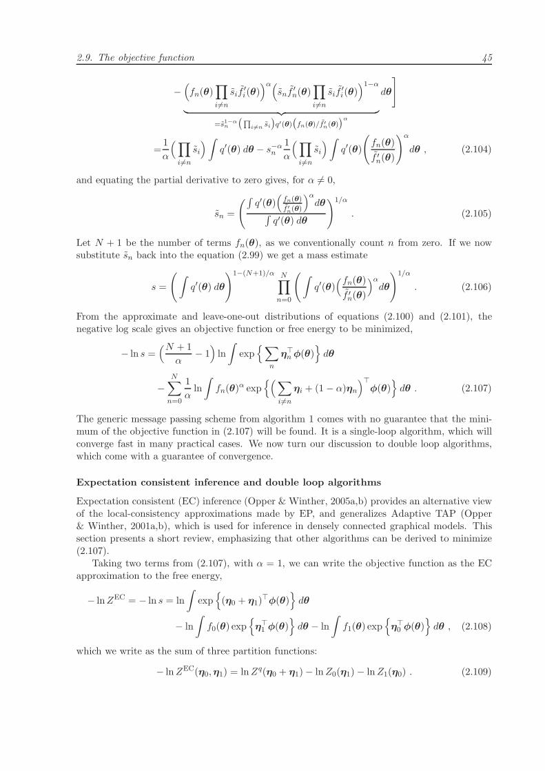
2.9. The objective function 45

−(

fn(θ)∏

i6=n

sif′i(θ)

)α(

snf′n(θ)

∏

i6=n

sif′i(θ)

)1−α

︸ ︷︷ ︸

=s1−αn

(Q

i6=n si

)q′(θ)

(fn(θ)/f ′

n(θ))α

dθ

]

=1

α

(∏

i6=n

si

) ∫

q′(θ) dθ − s−αn

1

α

(∏

i6=n

si

)∫

q′(θ)

(

fn(θ)

f ′n(θ)

)α

dθ , (2.104)

and equating the partial derivative to zero gives, for α 6= 0,

sn =

(∫q′(θ)

(fn(θ)

f ′n(θ)

)αdθ

∫q′(θ) dθ

)1/α

. (2.105)

Let N + 1 be the number of terms fn(θ), as we conventionally count n from zero. If we nowsubstitute sn back into the equation (2.99) we get a mass estimate

s =

(∫

q′(θ) dθ

)1−(N+1)/α N∏

n=0

(∫

q′(θ)(fn(θ)

f ′n(θ)

)αdθ

)1/α

. (2.106)

From the approximate and leave-one-out distributions of equations (2.100) and (2.101), thenegative log scale gives an objective function or free energy to be minimized,

− ln s =(N + 1

α− 1)

ln

∫

exp{∑

n

η⊤n φ(θ)

}

dθ

−N∑

n=0

1

αln

∫

fn(θ)α exp{(∑

i6=n

ηi + (1− α)ηn

)⊤φ(θ)

}

dθ . (2.107)

The generic message passing scheme from algorithm 1 comes with no guarantee that the mini-mum of the objective function in (2.107) will be found. It is a single-loop algorithm, which willconverge fast in many practical cases. We now turn our discussion to double loop algorithms,which come with a guarantee of convergence.

Expectation consistent inference and double loop algorithms

Expectation consistent (EC) inference (Opper & Winther, 2005a,b) provides an alternative viewof the local-consistency approximations made by EP, and generalizes Adaptive TAP (Opper& Winther, 2001a,b), which is used for inference in densely connected graphical models. Thissection presents a short review, emphasizing that other algorithms can be derived to minimize(2.107).

Taking two terms from (2.107), with α = 1, we can write the objective function as the ECapproximation to the free energy,

− lnZEC = − ln s = ln

∫

exp{

(η0 + η1)⊤φ(θ)

}

dθ

− ln

∫

f0(θ) exp{

η⊤1 φ(θ)

}

dθ − ln

∫

f1(θ) exp{

η⊤0 φ(θ)

}

dθ , (2.108)

which we write as the sum of three partition functions:

− lnZEC(η0,η1) = lnZq(η0 + η1)− lnZ0(η1)− lnZ1(η0) . (2.109)

46 2. Deterministic Approximate Inference

This can naturally be extended to a higher number of terms. By writing three distributions,

q(θ) =1

Zq(η0 + η1)exp

{

(η0 + η1)⊤φ(θ)

}

(2.110)

q0(θ) =1

Z0(η1)f0(θ) exp

{

η⊤1 φ(θ)

}

(2.111)

q1(θ) =1

Z1(η0)f1(θ) exp

{

η⊤0 φ(θ)

}

, (2.112)

the objective function in (2.109) is maximized by solving a nonlinear set of equations such thatthe moments match,

⟨φ(θ)

⟩

q=⟨φ(θ)

⟩

q0=⟨φ(θ)

⟩

q1. (2.113)

In this case we can view EP as a particular algorithm, and compare it to a double loop algorithm,for example given below.

To examine the stationary points of (2.109), notice that the log partition functions, forexample lnZ0, are the cumulant generating function of the random variables φ(θ),

H0 =∂2 lnZ0(η1)

∂η1∂η⊤1

=⟨φ(θ)φ(θ)⊤

⟩−⟨φ(θ)

⟩⟨φ(θ)

⟩⊤, (2.114)

where the expectations are taken under distribution q0(θ). The log partition functions aredifferentiable and convex functions of their domains. We can similarly define Hessian matricesHq and H1, all of which will be positive semi-definite. By considering η = (η0,η1), we canconclude that the EC objective function is a non-convex combination of convex functions, andhas a Hessian that is not necessarily positive semi-definite,

HEC =∂2 lnZEC(η)

∂η∂η⊤ = −(

Hq −H1 Hq

Hq Hq −H0

)

. (2.115)

There may therefore be more than one stationary point.The double loop algorithm (Yuille, 2002; Opper & Winther, 2005a) is guaranteed to converge

to a stationary point, assuming that a certain cost function is bounded from below. Defineηsum = η0 + η1, so that (2.109) is restated as

− lnZEC(ηsum,η1) = lnZq(ηsum)− lnZ0(η1)− lnZ1(ηsum − η1) . (2.116)

The double loop algorithm iterates two steps:

Step 1. When ηsum is held fixed, (2.116) is concave in η1, and can be uniquely maximized with

η1(t) = arg maxη1

[

− lnZEC(ηsum(t−1),η1)]

. (2.117)

As a result the moments of q0(t)(θ) and q1(t)(θ) are set to be equal,

⟨φ(θ)

⟩

q0(t)=⟨φ(θ)

⟩

q1(t). (2.118)

Step 2. When η1 is held fixed, (2.116) is a sum of a concave and a convex function of ηsum,and cannot be directly minimized. What we can do, however, is to update ηsum given themoments at a fixed η1. This is essentially an EP step, saying

q(t)(θ) = arg minq(θ)

KL(q0(t)(θ) ‖ q(θ)) , (2.119)

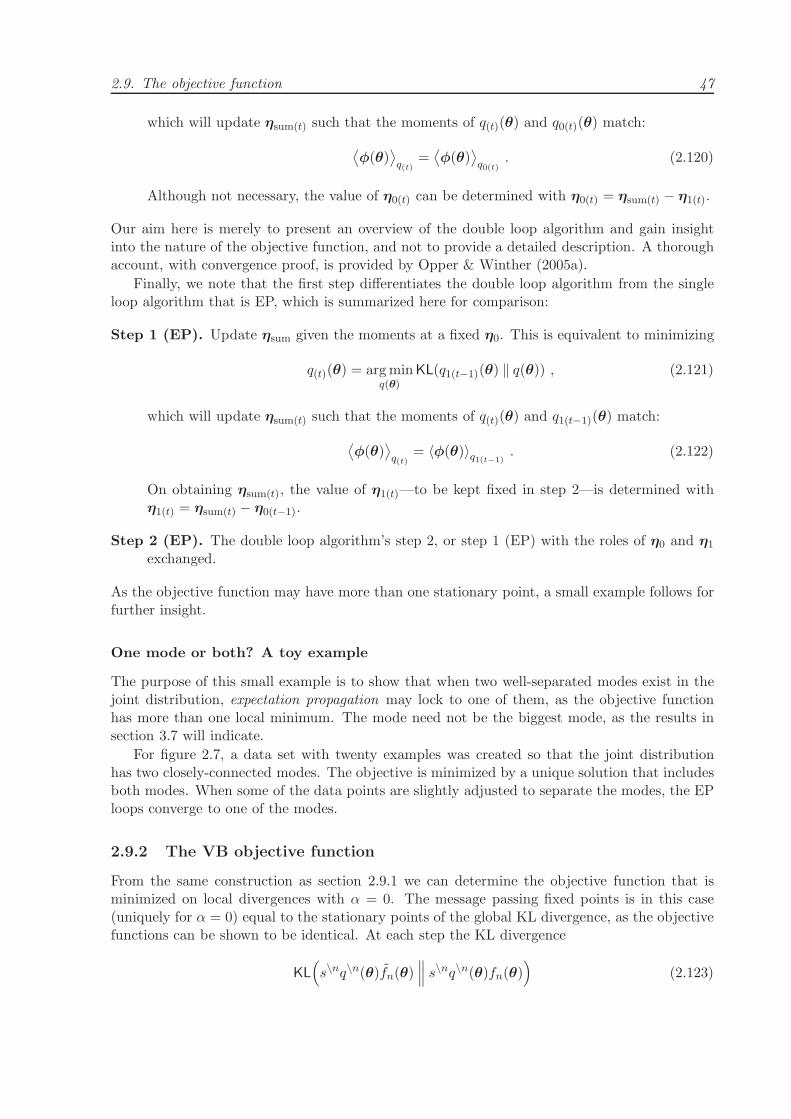
2.9. The objective function 47

which will update ηsum(t) such that the moments of q(t)(θ) and q0(t)(θ) match:

⟨φ(θ)

⟩

q(t)=⟨φ(θ)

⟩

q0(t). (2.120)

Although not necessary, the value of η0(t) can be determined with η0(t) = ηsum(t) − η1(t).

Our aim here is merely to present an overview of the double loop algorithm and gain insightinto the nature of the objective function, and not to provide a detailed description. A thoroughaccount, with convergence proof, is provided by Opper & Winther (2005a).

Finally, we note that the first step differentiates the double loop algorithm from the singleloop algorithm that is EP, which is summarized here for comparison:

Step 1 (EP). Update ηsum given the moments at a fixed η0. This is equivalent to minimizing

q(t)(θ) = arg minq(θ)

KL(q1(t−1)(θ) ‖ q(θ)) , (2.121)

which will update ηsum(t) such that the moments of q(t)(θ) and q1(t−1)(θ) match:

⟨φ(θ)

⟩

q(t)= 〈φ(θ)〉q1(t−1)

. (2.122)

On obtaining ηsum(t), the value of η1(t)—to be kept fixed in step 2—is determined withη1(t) = ηsum(t) − η0(t−1).

Step 2 (EP). The double loop algorithm’s step 2, or step 1 (EP) with the roles of η0 and η1

exchanged.

As the objective function may have more than one stationary point, a small example follows forfurther insight.

One mode or both? A toy example

The purpose of this small example is to show that when two well-separated modes exist in thejoint distribution, expectation propagation may lock to one of them, as the objective functionhas more than one local minimum. The mode need not be the biggest mode, as the results insection 3.7 will indicate.

For figure 2.7, a data set with twenty examples was created so that the joint distributionhas two closely-connected modes. The objective is minimized by a unique solution that includesboth modes. When some of the data points are slightly adjusted to separate the modes, the EPloops converge to one of the modes.

2.9.2 The VB objective function

From the same construction as section 2.9.1 we can determine the objective function that isminimized on local divergences with α = 0. The message passing fixed points is in this case(uniquely for α = 0) equal to the stationary points of the global KL divergence, as the objectivefunctions can be shown to be identical. At each step the KL divergence

KL

(

s\nq\n(θ)fn(θ)∥∥∥ s\nq\n(θ)fn(θ)

)

(2.123)

48 2. Deterministic Approximate Inference

µ1

µ2

(a) A joint distribution with twoclosely connected modes, createdfrom a data set with N = 20 exam-ples, is shown in red. In black is theEP solution, including both modes.Note: this is not the global KL so-lution.

µ1

µ2

(b) The joint distribution from thesame data set as figure 2.7(a) is shownhere, except that four of the datapoints (and hence likelihood terms)were slightly adjusted to allow EP tosettle on one mode and break symme-try.

Figure 2.7: One mode or both? As the modes in the joint (or posterior) distribution become moreseparated, EP here chooses one of them.

is minimized over fn(θ). With the cavity distribution defined as s\nq\n(θ) =∏

i6=n sif′i(θ), and

shorthand q′(θ) =∏

n f′n(θ), and can write the derivative with respect to an individual scale as

∂KL

∂sn=

∂

∂sn

[

sn

(∏

i6=n

si

)∫

q′(θ) lnsnf

′n(θ)

fn(θ)dθ

− sn

(∏

i6=n

si

) ∫

q′(θ) dθ +

∫

fn(θ)∏

i6=n

sifi(θ) dθ

]

= ln sn

(∏

i6=n

si

)∫

q′(θ) dθ +(∏

i6=n

si

)∫

q′(θ) lnf ′n(θ)

fn(θ)dθ . (2.124)

If the above expression is set to zero we find

sn = exp

{∫q′(θ) ln fn(θ)

f ′n(θ)

dθ∫q′(θ) dθ

}

. (2.125)

If sn is now substituted back into the equation (2.99), and the chosen factorizations p(x,θ) =∏

n fn(θ) and q′(θ) =∏

n f′n(θ) used, we get a mass estimate

s = exp

{∫q′(θ)

∑

n ln fn(θ)

f ′n(θ)

dθ∫q′(θ) dθ

}∫

q′(θ) dθ = exp

{∫q′(θ) ln p(x,θ)

q′(θ) dθ∫q′(θ) dθ

}∫

q′(θ) dθ . (2.126)

The objective function, as a function of the parameters of the exponential term approximations,is therefore

− ln s = −∫

exp{ N∑

n=0

η⊤n φ(θ)

} N∑

n=0

lnfn(θ)

exp{ηnφ(θ)} dθ/∫

exp{ N∑

n=0

η⊤n φ(θ)

}

dθ

2.9. The objective function 49

− ln

∫

exp{ N∑

n=0

η⊤n φ(θ)

}

dθ . (2.127)

To see that the objective function is equivalent to that of the global KL divergence, all weneed to do is notice that q′(θ) = cq(θ) for some constant c, such that q(θ) is a normalizeddistribution (in particular, from (2.99) the scale is s/

∏

n sn). Substituting q′(θ) = cq(θ) into(2.126) gives

s = exp

{∫

q(θ) lnp(x,θ)

q(θ)dθ

}

, (2.128)

which is exactly the scale or negative exponentiated free energy that we get when minimizingthe KL with VB.

2.9.3 Message passing with α = 0 as an EM algorithm

The generic message passing algorithm used to minimize local divergences over a factor graphrelies on a specific factorization of the joint distribution of interest. Uniquely for α = 0, theobjective function of message passing with local divergences and the global divergence objectivefunction will match, and the same stationary points will be reached. Using Jensen’s inequalitywe find a lower bound to the marginal likelihood in the usual way,

ln p(x) ≥∫

q(θ)q(z) lnp(x, z|θ)p(θ)

q(θ)q(z)dθdz

=

∫

q(θ)q(z) lnp(x, z|θ)

q(z)+

∫

q(θ) lnp(θ)

q(θ)dθ = F [q(θ), q(z)] . (2.129)

From the assumption that the observations are independent and identically distributed, thefactorization q(z) =

∏

n q(zn) can be made. In this case it is well known (Neal & Hinton,1998) that an incremental algorithm that updates one q(zn) at a time should increase F (theiralgorithm 7). In all their algorithms, the entire vector θ is updated in the M step.

EM and generic message passing routines

When the E-step updates a single q(zn), and the M-step updates q(θ), then F increases, as weare doing gradient ascent over functions (distributions). We may ask,

will the increase still hold if we factorize q(θ) into a product of functions over θ, andupdate only one of them in the M-step?

It turns out that this is indeed true, provided each factor i in the product can be defined as

fi(θ) ∝ exp{∫

q(zi) ln p(xi, zi|θ) dzi

}

. (2.130)

which only depends on q(zi).

Before presenting a formal argument of this result, a practical example is presented: Figure2.8 illustrates this behaviour in practice on the galaxy data set from section 3.7. An assumeddensity filtering (ADF) loop—essentially the first EP loop, which includes factors one by oneinto the approximation—was run to initialize all terms fn(θ). On initialization, the conditiongiven in (2.130) doesn’t hold for any of the factors, and ln s doesn’t show a monotonic increase.

50 2. Deterministic Approximate Inference

50 100 150 200 250 300 350 400−255

−250

−245

−240

−235

lns

Factor refinements

α = 0

BA

Figure 2.8: The galaxy data set from section 3.7 is used to illustrate that the objective function Fonly increases monotonically when (2.130) holds for all factors. The figure also indicates: A, the end ofthe ADF loop to get an initialization; B, the factor refinements with α = 0 where (2.130) holds.

As soon as (2.139) holds for all factors—which can be seen in the figure after one α = 0 loop—the objective function monotonically increases, even with partial updates to q(θ). If we solvefor ln s separately in each case, using the present q(θ)q(z) in

ln s = −KL(q(θ)q(z)

∥∥ p(θ, z|x)

)+ ln p(x) , (2.131)

we are still not guaranteed a monotonic increase until (2.130) holds, as figure 2.9 illustrates forthe same problem.

To determine formally when F will always increase, write

q(θ) =M∏

m=1

tm(θ) , (2.132)

for some factorization of the approximation, and assume q(θ) integrates to one. Let this beany factorization—we subscript it with m to indicate that it needn’t be over individual datalikelihoods.

Now write F [q] as (from i.i.d. assumption)

F [q] =

N∑

n=1

∫ M∏

m=1

tm(θ)q(zn) lnp(xn, zn|θ)

q(zn)dθdzn +

∫ M∏

m=1

tm(θ) lnp(θ)

∏Mm=1 tm(θ)

dθ . (2.133)

If we set ∂F/∂q(zn) to zero, we arrive at the familiar expression

q(zn) ∝ exp{∫

q(θ) ln p(xn, zn|θ) dθ}

, (2.134)

where Lagrange multipliers would give the correct normalization (there is an integration con-straint to keep q(zn) as a distribution). This is the particular E-step in the subproblem that issolved by the message passing scheme. The present factorized approximation

∏

m tm(θ) is used,and we find that the objective function increases.

Now take the functional derivative with respect to one of the m terms, with an addedintegration constraint through a Lagrange multiplier ℓ,

∂F∂ti(θ)

=∂

∂ti(θ)

[∫ M∏

m=1

tm(θ)q(z) lnp(x, z|θ)

q(z)dθdz +

∫ M∏

m=1

tm(θ) ln p(θ) dθ

2.9. The objective function 51

50 100 150 200 250−1800

−1600

−1400

−1200

−1000

−800

−600

−400

−200

0

lns

Factor refinements

α = 0

Figure 2.9: This graph zooms out on figure 2.8 to show the approximation ln s as the lower line, if thepresent q(θ) is used in (2.131). The large difference in the first α = 0 loop (an ADF loop was used toinitialize the approximation) is due to the fact that (2.131) ensures a lower bound to the joint p(x,θ).If the present approximation is relatively wide, a small scale is needed to ensure that the bound holds.As soon as (2.130) holds at the end of the first α = 0 loop, the message passing scale and the scaledetermined from (2.131) match.

−M∑

k=1

∫ M∏

m=1

tm(θ) ln tk(θ) dθ

]

+ ℓ∂

∂ti(θ)

[∫ M∏

m=1

tm(θ) dθ − 1

]

=∏

m6=i

tm(θ)

[∫

q(z) lnp(x, z|θ)

q(z)dz + ln p(θ)− ln ti(θ)− ln

∏

m6=i

tm(θ) + (ℓ− 1)

]

.

(2.135)

The above derivative is equated to zero and solved, hence

ti(θ)∏

m6=i

tm(θ) = p(θ) exp{∫

q(z) ln p(x, z|θ) dz}

exp{

−∫

q(z) ln q(z) dz}

exp{ℓ− 1} .

(2.136)Integrating on both sides (the left hand side is one), taking logs, solving for ℓ, and substitutingback, gives

ti(θ)∏

m6=i

tm(θ) = p(θ)exp{

∫q(z) ln p(x, z|θ) dz}

∫exp{

∫q(z) ln p(x, z|θ) dz} dθ . (2.137)

We are again on familiar territory, as the left hand side equals q(θ). But now only one factorti(θ) is updated, and the rest is left fixed. The update will still give coordinate ascent, but weneed to show an equivalence with the message passing formulation.

To see an equivalence with the generic message passing algotihm, let m ≡ n, so that theapproximate factors are therefore fn(θ) ∝ tn(θ)q(zn). From the i.i.d. assumption we have,

ti(θ)∏

n 6=i

tn(θ) =1

Zz

p(θ)∏

n 6=i

exp{∫

q(zn) ln p(xn, zn|θ) dzn

}

exp{∫

q(zi) ln p(xi, zi|θ) dzi

}

.

(2.138)

52 2. Deterministic Approximate Inference

If we choose t0(θ) ∝ p(θ) and tn(θ) ∝ exp{∫q(zn) ln p(xn, zn|θ) dzn} for n 6= i, the product

∏

n 6=i tn(θ) divides away on both sides, and the update simplifies to

ti(θ)∏

n 6=i

tn(θ) ∝ t0(θ)∏

n 6=i

tn(θ) exp{∫

q(zi) ln p(xi, zi|θ) dzi

}

ti(θ) ∝ exp{∫

q(zi) ln p(xi, zi|θ) dzi

}

, (2.139)

which only depends on q(zi). This is the key, as the full derivative simplifies as

dFdti(θ)

=∂F∂ti(θ)

+

N∑

n=1

∂F∂q(zn)

∂q(zn)

∂ti(θ)

=∂F∂ti(θ)

+∂F∂q(zi)

∂q(zi)

∂ti(θ). (2.140)

In the E-step ∂F/∂q(zi) was set to zero (and hence the derivative ∂q(zi)/∂ti(θ) need not be de-termined). Setting the partial derivative with respect to ti(θ) to zero should ensure a monotonicincrease of F .

Similar algorithms

We are not forced to choose m to match n, but can choose each ti(θ) to match any set ofdata items Ai, on the condition that the E-step sets ∂F/∂q(zn) = 0 for all n ∈ Ai. For thevariational Bayes EM algorithm the choice Ai = {1, . . . ,N} was made, with only one term ti.For the generalized message passing algorithm above the choice Ai = {i} was implemented,and we had N terms ti. Any grouping of data items to terms is therefore possible. All thesealgorithms are possible because the use of the exclusive KL divergence allows them to haveidentical objective functions.

Finding θML through message passing

In relation to the generic message passing algorithm, Neal & Hinton (1998)’s EM algorithm 9 isof particular interest, and it is briefly described here. It is used to find the maximum likelihoodparameter setting.

When the complete data likelihood p(x, z|θ) falls in the exponential family, its sufficientstatistics can be summarized as a sum of ‘sufficient statistics contributions’ from the individ-ual likelihoods p(xn, zn|θ) ∝ exp{η⊤

n φ(xn, zn)}, for n = 1, . . . ,N . Notice that the sufficientstatistics are for the complete likelihoods, and will include responsibilities for each example.Therefore, if p(x, z|θ) ∝ exp{η⊤φ(x, z)}, where η =

∑Nn=1 ηn, the maximum likelihood param-

eters θML can be found by iteratively updating data contributions until the parameter estimateconverges, akin to what we have done in the generic message passing algorithm. This is done asfollows:

In looping over all data points, assume that we are updating data point n at time t. For data

point n, we automatically copy η(t−1)i to η

(t)i , for all i 6= n. Given the parameter value θ(t−1)

from the previous iteration, set η(t)n to the sufficient statistics of p(xn, zn|θ(t−1)). The sufficient

statistics of the complete data likelihood is updated with η(t) = η(t−1) − η(t−1)n + η

(t)n . Finally

we set θ(t) to the θ of maximum likelihood given η(t).

2.10. Summary 53

2.10 Summary

This chapter introduced the α-divergence as a measure of distance between two possibly un-normalized probability distributions. This divergence is typically not tractable, but can beapproximately minimized if a particular factorization (or factor graph) of the distribution isconsidered, and the minimization restricted to local computations on the factor graph. Thisdistributed algorithm is not guaranteed to converge, although it often does and performs wellin practice.

A simple mixture of Gaussians was taken as a illustrative running example, and its fullmultivariate case is taken next as a practical case in chapter 3.

Chapter 3

Approximate inference formultivariate mixtures

3.1 Introduction

The message passing algorithms for approximate inference, as discussed in chapter 2, can bedirectly extended to a multivariate mixture of Gaussians. Many of the algorithms and derivationspresented here directly follow from those in chapter 2, and this chapter is meant to be read inconjunction with its predecessor.

Variational methods (α = 0) for mixtures of Gaussians have proved to be worth their saltto the machine learning community, with the work of Attias (2000) leading a wealth of ap-plications. The way has been paved for expectation propagation (α = 1) by Minka (2001a)’s‘clutter problem’ and treatment of mixtures with unknown weights. Subsequent work includedan application of EP to infinite mixtures with known variances (Minka & Ghahramani, 2003).Chang et al. (2005) used EP for Gaussian mixtures with independent dimensions, with addedparameters to determine whether a dimension was relevant to the clustering of the data.

New algorithms for mixture modeling

This chapter adds two new approaches to inference for a full multivariate mixture of Gaussians,namely EP and the more general α-divergence message passing scheme. We present a convincingargument for why and when EP should be favoured above VB, but also illustrate when thereis little to choose between the two algorithms, leaving a practitioner to his personal preference.This is followed in section 3.7 with a presentation of experimental results on a number of datasets, comparing the approximate predictive distributions and log marginal likelihoods with theresults obtained from VB and parallel tempering. Parallel tempering is a state of the art MCMCmethod, and will be further discussed in chapter 4. From this comparison we can gather thatthe approximate methods are perfectly suitable for model selection, and approximating thepredictive distribution with high accuracy. It is also practically shown that the EP fixed pointsare not necessarily unique, and a fixed point may depend on both the initialization and therandom order in which factor refinements take place. Both these questions were posed by Minka(2001a). Other points underlined empirically are: the log marginal likelihood estimates increasewith α; the number of local solutions depends on the prior width; the discrepancy between theapproximate and true log marginal likelihoods increase with model size; the marginal likelihoodsgive a characteristic ‘Ockham hill’ as model size increase, providing a useful tool for modelselection.

56 3. Approximate inference for multivariate mixtures

3.2 Mixture of Gaussians

Deterministic approximate inference for a multivariate mixture of Gaussians— where the mixingweights, means, and precision matrices are unknown—naturally arises as an extension of theexample in chapter 2. The unknown parameters are θ ≡ {π,µ,Λ} ≡ {πj ,µj ,Λj}Jj=1, with themixing weights πj summing to one. The likelihood of observing a single data point is

p(xn|µ,Λ,π) =

J∑

j=1

πjN (xn|µj ,Λ−1j ) , (3.1)

and under an assumption that the data is independent and identically distributed, the likelihoodof the data set is the product of the individual likelihoods.

For the likelihood, we choose conjugate priors, meaning that the posterior distribution will bein the same family as our choice of prior. Therefore, let the prior on the mixing weights and com-ponent parameters be Dirichlet and Normal-Wishart respectively. The choice of approximatingdistribution q will also match the form of the prior distribution.

The Dirichlet distribution is defined, for nonnegative δj , as

D(π|δ) =Γ(∑J

j=1 δj)∏J

j=1 Γ(δj)

J∏

j=1

πδj−1j =

1

ZD(δ)

J∏

j=1

πδj−1j . (3.2)

The Normal and Wishart distributions, where we keep the notation to that of Normal-Wishartto follow in (3.5), are defined as

N(µj|mj , (vjΛj)

−1)

=( vj

2π

) d2 |Λj |

12 exp

{

− 1

2tr[(µj −mj)(µj −mj)

⊤vjΛj ]}

(3.3)

W(Λj |aj ,Bj) =|Bj |aj

∏di=1 Γ(aj + 1−i

2 )π

−d(d−1)4 |Λj |aj− d+1

2 exp{

− tr[BjΛj]}

. (3.4)

The Wishart’s parameterization here is slightly unorthodox, but is chosen so that the one-dimensional case will exactly reduce to the Gamma distribution, G(λj |aj , bj) = b

aj

j /Γ(aj) ·λ

aj−1j e−bjλj . The Normal-Wishart distribution is defined as

NW(µj ,Λj |mj , vj , aj ,Bj) = N(µj |mj , (vjΛj)

−1)W(Λj |aj ,Bj)

=1

ZNW (vj , aj ,Bj)exp

{

− 1

2vjµ

⊤j Λjµj + vjm

⊤j Λjµj

− tr[(Bj +1

2vjmjm

⊤j )Λj ] + (aj −

d

2) ln |Λj |

}

(3.5)

ZNW

(vj , aj ,Bj) =(2π

vj

) d2π

d(d−1)4

∏di=1 Γ(aj + 1−i

2 )

|Bj |aj. (3.6)

Let the prior for the components, as well as the approximating distribution, be factorizedNormal-Wisharts,

p(µ,Λ) =J∏

j=1

NW(µj ,Λj |m0j , v0j , a0j ,B0j) and q(µ,Λ) =J∏

j=1

NW(µj ,Λj |mj , vj , aj ,Bj) .

(3.7)

3.3. Expectation propagation: a single observation 57

N

zn

π

µ

m0, v0

xn

Λ

δ0

a0,B0

π

µ

Λ

N

xn

znδ0

m0, v0

a0,B0

f0(π, µ,Λ)fn(π, µ,Λ, zn)

Figure 3.1: The Bayesian network, illustrating the parameter dependencies for a mixture of Gaussians,is shown on the left. The joint distribution was in this case completed with latent variables zn. Fromthe Bayesian network we can choose a particular factorization, as illustrated in the factor graph on theright. The factor graph clarifies the dependence of the factors on the different variables.

For a convenient notation, the parameters of the prior distribution are subscripted with anadditional ‘0’, and we assume that these hyperparameters are fixed, as illustrated in figure 3.1.The parameters of the approximating distribution are given without an additional subscript ‘0’,and it is these parameters that we will adjust to find a good approximating distribution q. Theprior for the mixing weights, as well as the relevant approximating distribution, is chosen to beDirichlet,

p(π) = D(π|δ0) and q(π) = D(π|δ) . (3.8)

We will therefore approximate the joint distribution p(x,θ) ≡ p(x,π,µ,Λ) by sq(µ,Λ)q(π).When a divergence measure other than setting α to one is chosen, say for example in variationalBayes, the likelihood is completed with latent variables z, and the joint distribution p(x, z,θ)will be approximated with sq(µ,Λ)q(π)q(z).

3.3 Expectation propagation: a single observation

We embark on the EP road in exactly the same way as we have done in the simple casewith unknown means in chapter 2, by computing the exact marginal for the scale, and usingresponsibility-weighted moment-matching equations to find the parameter updates.

If we know which component generated the data point in question, the following integral willprove to be extremely useful. It is the normalizer on observing a data point, or the likelihoodaveraged over a specific Normal-Wishart prior,

pj(xn) =

∫

W(Λj |a0j ,B0j)

∫

N (µ|m0j , (v0jΛ0j)−1)N (xn|µj ,Λ

−1j ) dµj dΛj

= T(

xn

∣∣∣m0j ,

v0j + 1

v0j

2B0j

2a0j − d+ 1, 2a0j − d+ 1

)

. (3.9)

The full derivation of this integral is given in appendix A.6. Two more relations will prove usefulin later derivations in this section:

Γ(δ + 1) = δΓ(δ) (3.10)

Ψ(δ + 1) =d

dδln Γ(δ + 1) =

d

dδ[ln δ + ln Γ(δ)] =

1

δ+ Ψ(δ) . (3.11)

The gamma function Γ(δ) is defined as Γ(δ) =∫∞0 tδ−1e−tdt, and Ψ(δ) is the digamma function,

58 3. Approximate inference for multivariate mixtures

given by the logarithmic derivative of the gamma function,

Ψ(δ) =d

dδln Γ(δ) =

Γ′(δ)Γ(δ)

. (3.12)

The following exposition gives the scale and parameters for matching sq(θ) to a prior multipliedby a likelihood for one data point.

3.3.1 The scale

The scale is determined with s =∫p(xn,µ,Λ,π) dµ dΛ dπ, and the result

s =1

∑Jj=1 δ0j

J∑

k=1

δ0kpk(xn) , (3.13)

is derived in appendix A.3. Define the responsibilities to be used in sections 3.3.2 and 3.3.3 as

rnj =δ0jpj(xn)

∑Jk=1 δ0kpk(xn)

=

δ0jT(

xn

∣∣∣m0j ,

v0j + 1

v0j

2B0j

2a0j − d+ 1, 2a0j − d+ 1

)

J∑

k=1

δ0kT(

xn

∣∣∣m0k,

v0k + 1

v0k

2B0k

2a0k − d+ 1, 2a0k − d+ 1

). (3.14)

3.3.2 Parameter updates for the components

To get the weighed parameter updates for q(µ,Λ), the following expectations under a Normal-Wishart distribution are needed. In each case the ‘prior’ expectation (the expectation if weknow that component j has not generated observation xn), and the ‘posterior’ expectation (theexpectation if we do know that component j was responsible for generating observation xn), isgiven. The responsibilities (3.14) will blend these expectations when we match moments. Theexpectations, derived in appendix A.6, are

〈Λj〉 = a0jB−10j (3.15)

〈Λj |xn〉 =(

a0j +1

2

)[

B0j +1

2

v0j

v0j + 1(xn −m0j)(xn −m0j)

⊤]−1

(3.16)

〈ln |Λj |〉 =

d∑

i=1

Ψ(

a0j +1− i

2

)

− ln |B0j | (3.17)

〈ln |Λj | |xn〉 =d∑

i=1

Ψ(

a0j +1

2+

1− i2

)

− ln∣∣∣B0j +

1

2

v0j

v0j + 1(xn −m0j)(xn −m0j)

⊤∣∣∣ (3.18)

〈Λjµj〉 = 〈Λj〉m0j (3.19)

〈Λjµj |xn〉 = 〈Λj |xn〉v0jm0j + xn

v0j + 1(3.20)

〈µ⊤j Λjµj〉 =

d

v0j+ m⊤

0j〈Λj〉m0j (3.21)

〈µ⊤j Λjµj |xn〉 =

d

v0j + 1+(v0jm0j + xn

v0j + 1

)⊤〈Λj |xn〉

(v0jm0j + xn

v0j + 1

)

. (3.22)

In the same way as we have done for the one-dimensional component means in chapter 2, wecan derive the parameter updates by again minimizing the KL-divergence with respect to the

3.3. Expectation propagation: a single observation 59

different parameters of q(µ,Λ). The parameters {mj , vj , aj ,Bj}Jj=1 of q(µ,Λ) that minimizesKL(p(xn,µ,Λ,π)‖sq(µ,Λ)q(π)) are

mj = Λ−1j

[(1− rnj)〈Λjµj〉+ rnj〈Λjµj |xn〉

](3.23)

d

vj= (1− rnj)〈µ⊤

j Λjµj〉+ rnj〈µ⊤j Λjµj |xn〉 −m⊤

j Λjmj (3.24)

d∑

i=1

Ψ(

aj +1− i

2

)

− ln |Bj | = (1− rnj)〈ln |Λj |〉+ rnj〈ln |Λj ||xn〉 ≡ c2 (3.25)

ajB−1j = Λj = (1− rnj)〈Λj〉+ rnj〈Λj |xn〉 ≡ C1 . (3.26)

(Both C1 and c2 are merely shorthands to keep the Newton method that follows below concise.)

Solving for aj and Bj in equations (3.25) and (3.26)

We have, for constants C1 and c2, ajB−1j = C1 and

∑di=1 Ψ(aj + (1 − i)/2) − ln |Bj | = c2.

Furthermore, ln |ajI|− ln |Bj | = ln |C1|, and hence − ln |Bj | = ln |C1|−d ln aj. We can thereforesolve for aj with Newton’s method by writing (3.25) as

d∑

i=1

Ψ(

aj +1− i

2

)

− d ln aj + ln |C1| − c2 = 0 . (3.27)

As another shorthand, define constant c = c2 − ln |C1|, and let

g(aj) =

d∑

i=1

Ψ(

aj +1− i

2

)

− d ln aj − c (3.28)

g′(aj) =

d∑

i=1

Ψ′(

aj +1− i

2

)

− d

aj, (3.29)

where Ψ′(aj) is called the trigamma function, the first derivative of the digamma function. ForNewton’s method we choose an initial aj , and update it until convergence with

anewj = aj −

g(aj)

g′(aj)= aj

[

1−∑d

i=1 Ψ(aj + (1− i)/2) − d ln aj − caj∑d

i=1 Ψ′(aj + (1− i)/2) − d

]

. (3.30)

The Wishart distribution is only defined for aj > (d − 1)/2, and there is no guarantee thatour update equations will satisfy this constraint, because the gradient in the Newton-Raphsonmethod is taken only locally. The choice of a0j as an initial value of aj may be good, butcomes without guarantee: As the digamma function is concave and monotonically increasing forpositive arguments, a choice of an initial value larger than the solution may cause a negativeargument to be passed to the digamma function in the following iteration, causing havoc in theiterative scheme.

We can reparameterize the fixed point equation to only allow for permissible values withaj = exp{a′j}+ (d− 1)/2, and solve for a′j . Write equation (3.28) as a function of a′j, and divideby the derivative with respect to a′j to get an update for a′j

new. For brevity, define k = (d−1)/2.Some rearrangement allows the update in terms of aj to be multiplicative,

anewj = (aj − k) exp

{

−∑d

i=1 Ψ(aj + (1− i)/2) − d ln aj − c(aj − k)

∑di=1 Ψ′(aj + (1− i)/2) − d(aj − k)/aj

}

+ k . (3.31)

On convergence of the Newton-Raphson method, aj is used to solve for Bj in equation (3.26).

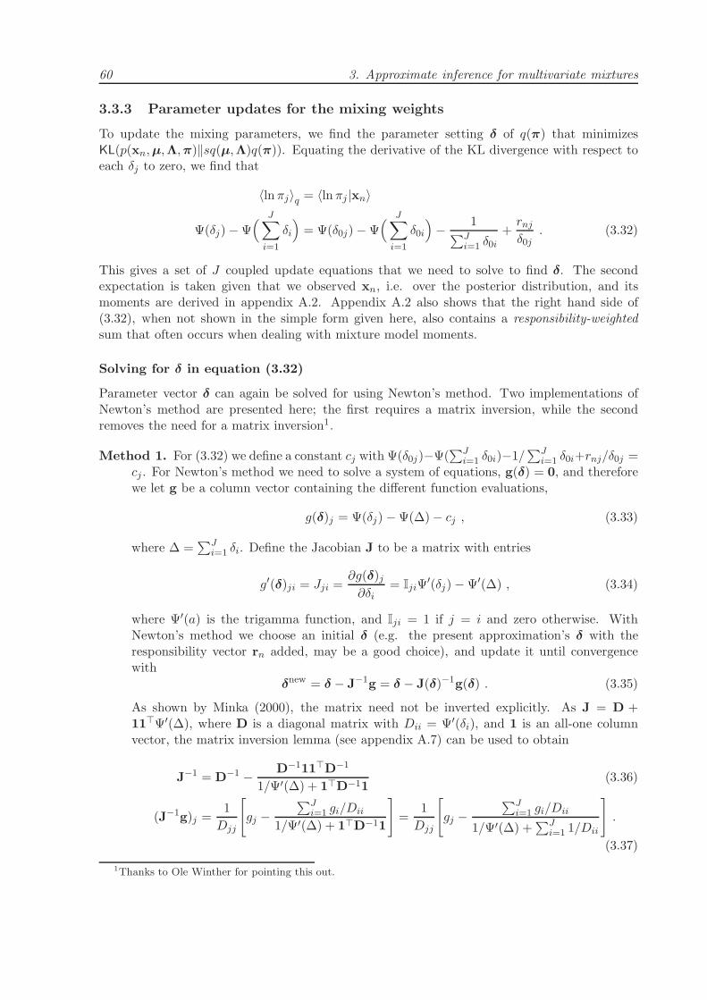
60 3. Approximate inference for multivariate mixtures

3.3.3 Parameter updates for the mixing weights

To update the mixing parameters, we find the parameter setting δ of q(π) that minimizesKL(p(xn,µ,Λ,π)‖sq(µ,Λ)q(π)). Equating the derivative of the KL divergence with respect toeach δj to zero, we find that

〈lnπj〉q = 〈lnπj |xn〉

Ψ(δj)−Ψ( J∑

i=1

δi

)

= Ψ(δ0j)−Ψ( J∑

i=1

δ0i

)

− 1∑J

i=1 δ0i

+rnj

δ0j. (3.32)

This gives a set of J coupled update equations that we need to solve to find δ. The secondexpectation is taken given that we observed xn, i.e. over the posterior distribution, and itsmoments are derived in appendix A.2. Appendix A.2 also shows that the right hand side of(3.32), when not shown in the simple form given here, also contains a responsibility-weightedsum that often occurs when dealing with mixture model moments.

Solving for δ in equation (3.32)

Parameter vector δ can again be solved for using Newton’s method. Two implementations ofNewton’s method are presented here; the first requires a matrix inversion, while the secondremoves the need for a matrix inversion1.

Method 1. For (3.32) we define a constant cj with Ψ(δ0j)−Ψ(∑J

i=1 δ0i)−1/∑J

i=1 δ0i+rnj/δ0j =cj . For Newton’s method we need to solve a system of equations, g(δ) = 0, and thereforewe let g be a column vector containing the different function evaluations,

g(δ)j = Ψ(δj)−Ψ(∆)− cj , (3.33)

where ∆ =∑J

i=1 δi. Define the Jacobian J to be a matrix with entries

g′(δ)ji = Jji =∂g(δ)j∂δi

= IjiΨ′(δj)−Ψ′(∆) , (3.34)

where Ψ′(a) is the trigamma function, and Iji = 1 if j = i and zero otherwise. WithNewton’s method we choose an initial δ (e.g. the present approximation’s δ with theresponsibility vector rn added, may be a good choice), and update it until convergencewith

δnew = δ − J−1g = δ − J(δ)−1g(δ) . (3.35)

As shown by Minka (2000), the matrix need not be inverted explicitly. As J = D +11⊤Ψ′(∆), where D is a diagonal matrix with Dii = Ψ′(δi), and 1 is an all-one columnvector, the matrix inversion lemma (see appendix A.7) can be used to obtain

J−1 = D−1 − D−111⊤D−1

1/Ψ′(∆) + 1⊤D−11(3.36)

(J−1g)j =1

Djj

[

gj −∑J

i=1 gi/Dii

1/Ψ′(∆) + 1⊤D−11

]

=1

Djj

[

gj −∑J

i=1 gi/Dii

1/Ψ′(∆) +∑J

i=1 1/Dii

]

.

(3.37)

1Thanks to Ole Winther for pointing this out.

3.4. Variational Bayes: a single observation 61

Method 2. Instead of solving for each δj in (3.32), we can solve for the digamma function oftheir sum, and from that recover each of the vector components. Define ∆ as the sum∑J

i=1 δi, so that we now have, for each j, Ψ(δj)− Ψ(∆) = cj . A unique expression for δjarises after taking the inverse of the digamma function,

δj = Ψ−1(cj + Ψ(∆)) . (3.38)

If we now sum over j in (3.38), and take both sides as arguments to the digamma function,the equation

Ψ(∆) = Ψ( J∑

j=1

Ψ−1(cj + Ψ(∆)))

(3.39)

can be used in Newton’s method to solve for Ψ(∆) in the usual way. Notice that a solutionis obtained for the digamma evaluation of ∆, and not ∆ itself, so that the solution can bedirectly substituted into (3.38). Let

g(Ψ(∆)

)= Ψ(∆)−Ψ

( J∑

j=1

Ψ−1(cj + Ψ(∆)))

(3.40)

g′(Ψ(∆)

)= 1−Ψ′

( J∑

j=1

Ψ−1(cj + Ψ(∆)))[

J∑

j=1

Ψ−1′(cj + Ψ(∆)))]

, (3.41)

so that

Ψ(∆)new = Ψ(∆)− g(Ψ(∆))

g′(Ψ(∆)). (3.42)

On solving for Ψ(∆), each δj can be recovered from (3.38).

3.4 Variational Bayes: a single observation

The introduction of latent allocation variables—turning the joint distribution into a product—allows the exclusive KL divergence KL(p(x, z,θ)‖sq(θ)q(z)) to be minimized with a well-knownEM algorithm. The joint distribution becomes a product with

p(xn,µ,Λ,π, zn) = p(xn|µ,Λ, zn)p(zn|π)p(π)p(µ,Λ)

=J∏

j=1

[πjp(xn|µj ,Λj)

]znjp(π)p(µ,Λ) . (3.43)

The joint can now be approximated with the factorized distribution sq(µ,Λ)q(π)q(zn), whereq(zn) is a multinomial distribution, q(zn) =

∏Jj=1 γ

znj

nj , with γnj ≥ 1 and∑

j γnj = 1.

3.4.1 Parameter updates

In a similar fashion to section 2.5, we get an iterative optimization scheme comprising of anexpectation and a maximization step.

E-step. For the expectation step the present approximation q(µ,Λ)q(π) in the loop is used,and the following holds:

∫

q(µ,Λ)q(π) ln p(xn, zn|µ,Λ,π) dµ dΛ dπ

62 3. Approximate inference for multivariate mixtures

=

J∑

j=1

znj

[

Ψ(δj)−Ψ( J∑

i=1

δi

)

+1

2

( d∑

i=1

Ψ(

aj +1− i

2

)

− ln |Bj |)

− 1

2(xn −mj)

⊤ajB−1j (xn −mj)−

1

2

d

vj− d

2ln 2π

]

. (3.44)

Equation (3.44) is used in updating the approximation q(zn) with

γnj = exp

{

Ψ(δj)−Ψ( J∑

i=1

δi

)

+1

2

( d∑

i=1

Ψ(

aj +1− i

2

)

− ln |Bj |)

− 1

2(xn −mj)

⊤ajB−1j (xn −mj)−

1

2

d

vj

}

, (3.45)

and finally γnj = γnj/∑

k γnk.

M-step. For the maximization step, we update the component parameters, for which we usethe prior, the data point xn, and the present approximation q(zn) (or γnj). Note that

∑

zn

q(zn) ln[p(xn, zn|µ,Λ,π)p(µ,Λ)p(π)

]

=

J∑

j=1

[

− 1

2

(

µj −v0jm0j + γnjxn

v0j + γnj

)⊤(v0j + γnj)Λj

(

µj −v0jm0j + γnjxn

v0j + γnj

)

− tr[(B0j +

1

2

v0jγnj

v0j + γnj(m0j − xn)(m0j − xn)⊤)Λj

]+(a0j +

γnj

2− d

2

)ln |Λj |

]

+J∑

j=1

(δ0j + γnj − 1) lnπj + const , (3.46)

and as this is in the Dirichlet and Normal-Wishart forms of (3.2) and (3.5) we can readoff the parameter updates as

vj = v0j + γnj (3.47)

mj =v0jm0j + γnjxn

v0j + γnj(3.48)

Bj = B0j +1

2

v0jγnj

v0j + γnj(m0j − xn)(m0j − xn)⊤ (3.49)

aj = a0j +γnj

2(3.50)

δj = δ0j + γnj . (3.51)

The iterations between the E and M steps are repeated until convergence, and convergence (atleast to a local minimum) is guaranteed because both steps are convex.

3.4.2 The scale

The approximate log marginal likelihood ln s—or the negative variational free energy—is com-puted after the iterative EM method has converged. As we can write ln p(xn,µ,Λ,π, zn) =

3.5. α-divergence: a single observation 63

ln p(xn|µ,Λ, zn) + ln p(zn|π) + ln p(π) + ln p(µ,Λ) we have

ln s = 〈ln p(xn|µ,Λ, zn)〉+ 〈ln p(zn|π)〉+ 〈ln p(π)〉+ 〈ln p(µ,Λ)〉− 〈ln q(µ,Λ)〉 − 〈ln q(π)〉 − 〈ln q(zn)〉 (3.52)

where the expectation is taken over the resulting approximation from the EM steps, q(µ,Λ)q(π)q(zn).To get ln s, an approximation to the log marginal likelihood, we simply determine these expec-tations. Notice the difference between prior parameters (starting with a subscript ‘0’), and theparameters of q, which go without the ‘0’ subscript. The expectations needed in (3.52) are

〈ln p(xn|µ,Λ, zn)〉 =⟨ J∑

j=1

znj ln p(xn|µj ,Λj)⟩

=1

2

J∑

j=1

γnj

[

− d ln(2π) +d∑

i=1

Ψ(

aj +1− i

2

)

− ln |Bj |

− (xn −mj)⊤ajB

−1j (xn −mj)−

d

vj

]

(3.53)

〈ln p(zn|π)〉 =⟨ J∑

j=1

znj lnπj

⟩

=J∑

j=1

γnj

[

Ψ(δj)−Ψ( J∑

i=1

δi

)]

(3.54)

〈ln p(π)〉 = lnZD(δ0) +

J∑

j=1

(δ0j − 1)[

Ψ(δj)−Ψ( J∑

i=1

δi

)]

(3.55)

〈ln p(µ,Λ)〉 =

J∑

j=1

[

− lnZNW

(v0j , a0j ,B0j)−d

2

v0j

vj− 1

2v0j(mj −m0j)

⊤ajB−1j (mj −m0j)

− ajtr[B0jB

−1j

]+(

a0j −d

2

)( d∑

i=1

Ψ(

aj +1− i

2

)

− ln |Bj |)]

(3.56)

〈ln q(µ,Λ)〉 =

J∑

j=1

[

− lnZNW

(vj , aj ,Bj)−d

2

− daj +(

aj −d

2

)( d∑

i=1

Ψ(

aj +1− i

2

)

− ln |Bj |)]

(3.57)

〈ln q(π)〉 = − lnZD(δ) +

J∑

j=1

(δj − 1)[

Ψ(δj)−Ψ( J∑

i=1

δi

)]

(3.58)

〈ln q(zn)〉 =

J∑

j=1

γnj ln γnj . (3.59)

3.5 α-divergence: a single observation

To minimize an α-divergence, we follow the fixed point framework from section 2.6. The ‘prior’ ineach step is the product [p(π)p(µ,Λ)]α [q(t)(π)q(t)(µ,Λ)]1−α, for which we define the shorthandparameters

vi = αv0i + (1− α)vi(t) (3.60)

64 3. Approximate inference for multivariate mixtures

mi =αv0im0i + (1− α)vi(t)mi(t)

αv0i + (1− α)vi(t)(3.61)

Bi = αB0i + (1− α)Bi(t) +1

2

α(1− α)v0ivi(t)

αv0i + (1− α)vi(t)(m0i −mi(t))(m0i −mi(t))

⊤ (3.62)

ai = αa0i + (1− α)ai(t) (3.63)

δj = αδ0j + (1− α)δj(t) . (3.64)

By examining the above parameters and the scale given in (3.66), we see that the scale may notbe finite, and we suddenly find ourselves with a set of practical constrains when α is outsidethe interval [0, 1]. Some of the parameter constraints needed to ensure that the approximatingdistribution is normalizable, might be violated:

• from (3.60), we require vi > 0;

• from (3.62), we require |Bk| > 0;

• from (3.63) and the Gamma functions in (3.65), we require both ak > (d − 1)/2 andak > (d− α)/2;

• from (3.64), we require δj ≥ 0.

The experimental results given in section 3.7 only consider α = 12 , the Hellinger distance, giving

approximations ‘between’ those arising from variational Bayes and expectation propagation. Forvalues of α > 1, the fixed point iterations often failed on account of the constraints given above.

3.5.1 Fixed point iterations

The iterative scheme outlined in section 2.6 is now implemented on a larger scale. We startwith an initial s(0)q(0)(zn)q(0)(π)q(0)(µ,Λ). The prior distribution may provide a good startingpoint, with the parameters γnj(0) of q(0)(zn) all set to 1/J , and s(0) set to one. Starting witht = 0, the following steps are repeated until convergence, or until some maximum number ofiterations is reached.

Step 1. Determine the scale, for which we define the unscaled responsibilities rnj as

Rnj = γ1−αnj(t)

Γ(δj + α)

Γ(δj)|Bj |(1−α)/2 Γ(

[2aj+α−d]2 )

Γ([2aj+α−d]+d

2 )

d∏

l=1

Γ(2aj+α+1−l

2 )

Γ(2aj+1−l

2 )

× T(

xn

∣∣∣ mj ,

vj + α

vjα

2Bj

2aj + α− d, 2aj + α− d)

, (3.65)

to get the scale,

s(t′) = s1−α(t)

1

ZD(δ0)α1

ZD(δ(t))1−α

( ∏

j Γ(δj)

Γ(α+∑J

j=1 δj)

)

×J∏

j=1

ZNW (vj , aj , Bj)

ZNW

(v0j , a0j ,B0j)αZNW(vj(t), aj(t),Bj(t))1−α

× (2π)(1−α)d/2α−d/2J∑

k=1

Rnk . (3.66)

3.5. α-divergence: a single observation 65

The derivation of the scale is given in appendix A.4.2; to check the correctness of thederivation, substituting α = 1 in the above scale again gives us the scale (3.13) derived forexpectation propagation.

Now we find a normalized distribution q(t′)(zn)q(t′)(π)q(t′)(µ,Λ) that minimizes the KLdivergence to

p(xn,µ,Λ,π, zn)α[q(t)(zn)q(t)(π)q(t)(µ,Λ)]1−α . (3.67)

Again, we have already solved for the scale and only need to match moments. The followingexpectations are derived in appendix A.6, will be used in the (responsibility-weighted)moment matching update equations:

〈Λj〉 = ajB−1j (3.68)

〈Λj |xn〉 =(

aj +α

2

)[

Bj +1

2

αvj

vj + α(xn − mj)(xn − mj)

⊤]−1

(3.69)

〈ln |Λj |〉 =

d∑

i=1

Ψ(

aj +1− i

2

)

− ln |Bj | (3.70)

〈ln |Λj | |xn〉 =

d∑

i=1

Ψ(

aj +α

2+

1− i2

)

− ln∣∣∣Bj +

1

2

αvj

vj + α(xn − mj)(xn − mj)

⊤∣∣∣

(3.71)

〈Λjµj〉 = 〈Λj〉mj (3.72)

〈Λjµj |xn〉 = 〈Λj |xn〉vjmj + αxn

vj + α(3.73)

〈µ⊤j Λjµj〉 =

d

vj+ m⊤

j 〈Λj〉mj (3.74)

〈µ⊤j Λjµj |xn〉 =

d

vj + α+( vjmj + αxn

vj + α

)⊤〈Λj |xn〉

( vjmj + αxn

vj + α

)

. (3.75)

For the responsibilities, define

rnj =Rnj

∑Jk=1Rnk

. (3.76)

Exactly the same weighted sum of moments as equations (3.23) to (3.26) will be used toupdate mj(t′), vj(t′), aj(t′) and Bj(t′) for all components j, and we do not repeat them here.The only difference lies in the computation of the expectations and responsibilities beingused.

By taking a similar route as that taken to derive the mixing weight updates in section3.3.3, we arrive at a set of update equations,

Ψ(δj(t′))−Ψ( J∑

i=1

δi(t′)

)

= (1− rnj)Ψ(δj) + rnjΨ(

δj + α)

−Ψ(

α+J∑

i=1

δi

)

= cj . (3.77)

The parameter values can be solved for with Newton’s method, following the method laidout in section 3.3.3, only with different values for cj .

Finally, the parameters of q(t′)(zn) are set as γnj(t′) = rnj .

66 3. Approximate inference for multivariate mixtures

Step 2. We have a scaled distribution s(t′)q(t′)(zn)q(t′)(π)q(t′)(µ,Λ), which we damp towardsthe previous approximation, s(t)q(t), to find an updated s(t+1)q(t+1), where q(t+1) is nor-malized. Define the parameters of the (unscaled) damped approximating distributionsq(t)(π)ǫq(t′)(π)1−ǫ and q(t)(µ,Λ)ǫq(t′)(µ,Λ)1−ǫ as

vj(t+1) = ǫvj(t) + (1− ǫ)vj(t′) (3.78)

mj(t+1) =ǫvj(t)mj(t) + (1− ǫ)vj(t′)mj(t′)

ǫvj(t) + (1− ǫ)vj(t′)(3.79)

Bj(t+1) = ǫBj(t) + (1− ǫ)Bj(t′) (3.80)

+1

2

ǫvj(t)(1− ǫ)vj(t′)

ǫvj(t) + (1− ǫ)vj(t′)(mj(t) −mj(t′))(mj(t) −mj(t′))

⊤ (3.81)

aj(t+1) = ǫaj(t) + (1− ǫ)aj(t′) (3.82)

δ(t+1) = ǫδ(t) + (1− ǫ)δ(t′) , (3.83)

for the mixing weights and each of the mixture components j. Then damping gives

q(t)(π)ǫq(t′)(π)1−ǫ =1

ZD(δ(t))ǫ1

ZD(δ(t′))1−ǫ

J∏

j=1

πδj(t+1)−1

j (3.84)

q(t)(µ,Λ)ǫq(t′)(µ,Λ)1−ǫ =

J∏

j=1

1

ZNW

(v(t), aj(t),Bj(t))ǫ1

ZNW

(v(t′), aj(t′),Bj(t′))1−ǫ

× exp{

− 1

2(µj −mj(t+1))

⊤(vj(t+1)Λj)(µj −mj(t+1))

− tr[Bj(t+1)Λj] +(aj(t+1) −

d

2

)ln |Λj |

}

(3.85)

q(t)(zn)ǫq(t′)(zn)1−ǫ =

J∏

j=1

[γǫnj(t)γ

1−ǫnj(t′)]

znj . (3.86)

We would like to keep q(t+1) as a normalized distribution, for which we need to divide itby some scale, and multiply s(t+1) by the same scale. The required scales are

Z1 =

∫

q(t)(π)ǫq(t′)(π)1−ǫ dπ =Z

D(δ(t+1))

ZD(δ(t))ǫZD(δ(t′))1−ǫ(3.87)

Z2 =

∫

q(t)(µ,Λ)ǫq(t′)(µ,Λ)1−ǫ dµ dΛ

=J∏

j=1

ZNW

(vj(t+1), aj(t+1),Bj(t+1))

ZNW (vj(t), aj(t),Bj(t))ǫZNW (vj(t′), aj(t′),Bj(t′))1−ǫ. (3.88)

Finally the parameters of q(t+1)(zn) are set as

γnj(t+1) = Z−13 γǫ

nj(t)γ1−ǫnj(t′) , where Z3 =

J∑

k=1

γǫnk(t)γ

1−ǫnk(t′) (3.89)

To keep q(t+1) as a normalized distribution, a division by Z1, Z2, and Z3 has to be made;therefore their logs are added to ln s(t+1) with

ln s(t+1) = ǫ ln s(t) + (1− ǫ) ln s(t′) + lnZ1 + lnZ2 + lnZ3 . (3.90)

3.6. Minimizing over a factor graph 67

3.6 Minimizing over a factor graph

For full multivariate mixtures we have chosen to work with Dirichlets (for the mixing weights)and Normal-Wisharts (for the component parameters) as approximating distributions. We letthe factor approximations fn be of exactly the same form,

fn(π,µ,Λ) = sn

J∏

j=1

exp{

(δnj − 1) ln πj −1

2vnjµ

⊤j Λjµj + vnjm

⊤njΛjµj

− tr[(Bnj +1

2vnjmnjm

⊤nj)Λj ] + (anj −

d

2) ln |Λj |

}

. (3.91)

This choice of fn also takes the same form as the prior. The message passing algorithm is:

• Start by initializing, for n = 1, . . . ,N , and all components j,

δnj = 1 mnj = 0 anj =d

2

vnj = 0 Bnj = 0 sn = 1 . (3.92)

so that all the factor approximations are one. Initialize the prior, for all j, as

δ0j = δ0j B0j = B0j

v0j = v0j a0j = a0j

m0j = m0j s0 =1

ZD(δ0)

J∏

j=1

1

ZNW

(v0j , a0j , B0j). (3.93)

• Repeat until all fn converge:

1. Pick a factor n. This can be done by looping over random permutations of 1, · · · ,N .

2. Compute the ‘old’ approximation q\n(π)q\n(µ,Λ), with parameters indexed by anadditional ‘o’, from reversing equations (3.101) to (3.105), hence subtracting thefactor contributions from the present approximation,

voj = vj − vnj (3.94)

moj =vjmj − vnjmnj

voj(3.95)

Boj = Bj − Bj +1

2vjmjm

⊤j −

1

2vojmojm

⊤oj −

1

2vnjmnjm

⊤nj (3.96)

aoj = aj − anj +d

2(3.97)

δoj = δj − δnj + 1 . (3.98)

If the cavity distribution q\n is not proper (normalizable), a robust heuristic wouldbe to skip the update and continue with the next factor in step 1. Figure 3.5 showsthe effect of these update skips.

3. Again let S, and for all j, δj , vj, j , aj , Bj be the parameters of q(π)newq(µ,Λ)new

that minimizes (2.84), in this particular case

Sq(π)newq(µ,Λ)new = arg mins′q(π)q(µ,Λ)

Dα

(q\n(π)q\n(µ,Λ)fn(π,µ,Λ)

∥∥ s′q(π)q(µ,Λ)

).

(3.99)

68 3. Approximate inference for multivariate mixtures

The new approximation can be found with the methods discussed in sections 3.3,3.4 and 3.5. Depending on the value of α, latent variables may need to be addedto the joint distribution for tractability, and q(zn) added to the approximation. Asthe parameters γnj of q(zn) are related to a specific term fn and its approximationfn, it is not necessary to keep track of any ‘leave-one-out’ distributions for the latentvariables, and they are merely used as a means to an end.

After solving for the new approximation, we have to set the factor contribution, andhence

fn = Sq(π)newq(µ,Λ)new

q\n(π)q\n(µ,Λ)

= SZ

D(δo)

ZD(δ)

J∏

j=1

ZNW

(voj , aoj ,Boj)

ZNW

(vj , aj ,Bj)

exp{

(δj − δoj) ln πj −1

2(vj − voj)µ

⊤j Λjµj + (vjmj − vojmoj)

⊤Λjµj

− tr[(Bj −Boj +1

2vjmjm

⊤j −

1

2vojmojm

⊤oj)Λj ] + (aj − aoj) ln |Λj |

}

. (3.100)

According to factor definition (3.91), we get the following substitutions for the dif-ferent parameter contributions,

vnj = vj − voj (3.101)

mnj =vjmj − vojmoj

vnj(3.102)

Bj = Bj −Boj +1

2vjmjm

⊤j −

1

2vojmojm

⊤oj −

1

2vnjmnjm

⊤nj (3.103)

anj = aj − aoj +d

2(3.104)

δnj = δj − δoj + 1 (3.105)

sn = SZ

D(δo)

ZD(δ)

J∏

j=1

ZNW

(voj , aoj ,Boj)

ZNW

(vj , aj ,Bj). (3.106)

• Finally we determine the approximation to the evidence p(x) with

p(x) ≈∫ N∏

n=0

fn(π,µ,Λ) dπ dµ dΛ

=( N∏

n=0

sn

) ∫ J∏

j=1

πPN

n=0 δnj−1j e−

12[PN

n=0 vnj ]µ⊤j Λjµj+[

PNn=0 vnjm

⊤nj ]Λjµj

× e−tr[PN

n=0(Bnj+12vnjmnjm

⊤nj)Λj ]+

PNn=0(anj− d

2) ln |Λj| dπ dµ dΛ

=( N∏

n=0

sn

) ∫ J∏

j=1

πδj−1j e−

12vjµ⊤

j Λjµj+vjm⊤j Λjµj

× e−tr[(Bj+12vjmjm

⊤j )Λj ]+(aj− d

2) ln |Λj | dπ dµ dΛ

=( N∏

n=0

sn

)

ZD(δ)

J∏

j=1

ZNW (vj , aj,Bj) . (3.107)

3.7. Experimental results 69

0 50 100 150 200 250 300 350−250

−200

−150

−100

−50

0

lns

Factor refinements

One loop overa random

ordering of thedata

Figure 3.2: For the galaxy data set, this plot shows the progress of the log marginal likelihood estimateover time. The first loop over N = 82 data points is the ‘assumed density filtering’ (ADF) loop, whereobservations are included one by one in the approximation. Further loops over random permutationsof the data cause the approximation to stabilize to ln s = −232.4. With three components, the priorparameter settings were δ0j = 1, m0j = 0, v0j = 10−2, a0j = 1 and B0j = 0.11.

Starting with another prior contribution

In the case of mixtures discussed here, a symmetric prior (i.e. the prior is identical for eachterm in the product over j) leaves the algorithm in a stationary point making no real progress,as all responsibilities rnj remain equal. We may wish to break symmetry by, for example,starting with a random factor initialization. Symmetry is broken here by starting with the‘wrong’ prior, and correcting the prior factor contributions to the true prior after a loop overthe data. After removing the (wrong) prior’s contribution to the approximation, we find thenew approximation’s parameters by including the (true) prior with

vj = voj + v0j (3.108)

mj =vojmoj + v0jm0j

vj(3.109)

Bj = Boj + B0j +1

2vojmojm

⊤oj +

1

2v0jm0jm

⊤0j −

1

2vjmjm

⊤j (3.110)

aj = aoj + a0j −d

2(3.111)

δj = δoj + δ0j − 1 , (3.112)

and hence the prior contributions are corrected to v0j = v0j , m0j = m0j , B0j = B0j , a0j =a0j , δ0j = δ0j . Lastly, the prior’s contribution to the scale or approximate marginal likelihood is

s0 =1

ZD(δ0)

J∏

j=1

1

ZNW

(v0j , a0j ,B0j). (3.113)

70 3. Approximate inference for multivariate mixtures

3.7 Experimental results

This section examines the approximate predictive distributions and log marginal likelihoodsfound by minimizing the VB, EP, and α = 1

2 energy (objective) functions over a factor graph,and the results are compared to the ‘gold standard’ predictions and marginal likelihoods obtainedfrom thermodynamic integration through parallel tempering. Parallel tempering is a Markovchain Monte Carlo method, discussed in greater detail in chapter 4.

Two methods for approximate inference that we discussed in chapter 1 are not included in thecomparison. The maximum a posteriori estimate is omitted, for it doesn’t provide an estimateof the probability mass and cannot be used for model selection. A Laplace approximation canbe used for model selection, as was done with flat priors by Roberts et al. (1998). It is excludedas the Hessian matrix couples the component means and variances into a joint covariance matrixof a Gaussian q(µj ,Λj), making the approximate predictive distribution intractable.

3.7.1 A toy example

Before turning to larger real-life data sets, we illustrate the difference between EP and VB on atoy example: EP generally gives better predictive distributions than VB on small data sets. Asmore data is observed, the scale of this improvement is expected to decrease.

Here a data set with N = 7 examples were generated from a two-component mixture ofGaussians, and by default we therefore know the correct model class. We have used priorparameter settings δ0j = 1, m0j = 0, v0j = 10−2, a0j = 1 and B0j = 0.11.

In figures 3.3(a) and 3.3(c) we show a marked difference between the VB and EP predictivedistributions on this small data set, both with an incorrect and correct choice of J . Notice thatEP gives a broader estimate of q(θ), and hence also broader predictive densities. This differenceis most noticeable around the peaks of the distributions, with EP generally giving a closer fit.

As a next illustration the size of the data set was doubled to N = 14 by duplicating eachexample. We expect less of a difference in predictive density as the posterior has more concen-trated (peaked) modes when there is a greater abundance of data. Figures 3.3(b) and 3.3(d)show a smaller—or even indistinguishable—discrepancy between the EP and VB predictive dis-tributions. In figure 3.3(b) we can still mark EP’s slight improvement around the peaks of thedensity.

EP gives a better approximation than VB to the log marginal likelihood. This can beexpected from the nature of the EP updates; also bear in mind that VB provides a lower boundto the true lnZ. This is illustrated in figure 3.4 for each of the problems in figure 3.3.

3.7.2 Experimental observations

A number of observations from the experiments presented here will confirm the theoretic resultsgiven in chapter 2:

• The log marginal likelihood estimates increase with α. The respective objective functionsare continuously related through parameter α (see for example equation (2.107)) andtherefore we expect related local minima for many data sets. This relation can be observed,with the evaluation of ln s increasing with α over a local minimum.

• The number of local solutions is influenced by the width of the prior distribution, withmore local minima arising in broader priors.

3.7. Experimental results 71

−2 −1.5 −1 −0.5 0 0.5 1 1.5 20

0.1

0.2

0.3

0.4

0.5

0.6

0.7

0.8

{xn}Nn=1MCMCEC/PVB

(a) J = 3, N = 7

−2 −1.5 −1 −0.5 0 0.5 1 1.5 20

0.2

0.4

0.6

0.8

1

1.2

{xn}Nn=1}MCMCEC/PVB

(b) J = 3, N = 14

−2 −1.5 −1 −0.5 0 0.5 1 1.5 20

0.1

0.2

0.3

0.4

0.5

0.6

0.7

0.8

0.9

1

{xn}Nn=1MCMCEC/PVB

(c) J = 2, N = 7

−2 −1.5 −1 −0.5 0 0.5 1 1.5 20

0.2

0.4

0.6

0.8

1

1.2

{xn}Nn=1MCMCEC/PVB

(d) J = 2, N = 14

Figure 3.3: The predictive densities p(xnew|x,MJ) given by expectation consistent inference (the ex-pectation propagation algorithm) and variational Bayes. In figures 3.3(a) and 3.3(c) a two-componenttoy data set was used. For figures 3.3(b) and 3.3(d) the data set size was doubled by duplicating eachexample. With less data EC/P gives a predictive density that is closer to the truth than VB. With in-creasing data set size (and hence also more sharply peaked posteriors) this difference becomes less markedto almost indistinguishable.

−12.5

−12

−11.5

−11

−10.5

−10

(a)

lnZ

−16.5

−16

−15.5

−15

−14.5

−14

(b)−11

−10.9

−10.8

−10.7

−10.6

−10.5

−10.4

−10.3

−10.2

−10.1

−10

(c)−14.5

−14.4

−14.3

−14.2

−14.1

−14

−13.9

−13.8

−13.7

−13.6

−13.5

(d)

MCMC

EC/P

VB

Figure 3.4: The log marginal likelihood estimates for the problems shown in figures 3.3(a) to 3.3(d).

72 3. Approximate inference for multivariate mixtures

• The EP fixed points are not unique, and the fixed point depends on both the initializationand the random order in which factor refinements take place. Both these questions wereposed by Minka at the end of his thesis (Minka, 2001a).

• The growth of ln s, as a function of model size, gives a characteristic ‘Ockham hill’, wherethe ‘peak’ of the hill indicates the model with highest approximate ln p(x). This graphcan be used for model comparison or selection, as its form closely matches the MCMCevaluation of ln p(x).

• The discrepancy between ln s and the true ln p(x) grows as the model size is increased. Thisis mainly due to mixtures being invariant under component relabelling, with the numberof permutations increasing as J !, with J being the number of components. The truelog marginal likelihood will take all such permutations—mostly giving different posteriormodes—into account. Provided the modes are well separated, the approximate distributionq(θ) is only able to capture a single.

• As component relabelling gives the same predictive distribution under a symmetric prior,we do not expect a pronounced difference between the true predictive distribution and thepredictive distribution obtained from an average over a single-mode q(θ).

• the EC/EP approximation gives a predictive distribution that is closer to the truth thanthat given by VB.

The message passing algorithm was run for α = 0 (VB) , α = 12 (Hellinger distance), and

α = 1 (EC/EP). The data sets under investigation have been well studied, e.g. by Richardson &Green (1997) for a reversible jump MCMC, and by Corduneanu & Bishop (2001) for variationalBayesian model selection:

galaxy. The galaxy data set contains the velocities (in 1000s of km/second) of 82 galaxies,diverging from our own, in the Corona Borealis region. Multimodal velocity densitiesprovides evidence for clustering of the galaxies into superclusters which are surrounded bylarge voids, with clusters corresponding to modes in the velocity density (Roeder (1990)provides more detail).

acidity. The acidity data set contains the log measured acid neutralizing capacity indices for155 lakes in North-central Wisconsin (USA). Identifying groups of lakes at different envi-ronmental risk can be useful in determining if any characteristics of a lake can be used topredict higher acidification.

enzyme. The enzyme data set contains enzymatic activity measurements, for an enzyme in-volved in the metabolism of carcinogenic substances, taken from 245 unrelated individuals.Of interest here is the identification of subgroups of slow or fast metabolisers as a markerof genetic polymorphism in a general population.

old faithful. The data set used contains 222 observations from the Old Faithful Geyser in theYellowstone National Park. Two measurements—the duration of an eruption, rounded tothe nearest 0.1 minutes, and the waiting time to the next eruption, rounded to the nearestminute—constitute a single observation. Although not the largest or most regular, it is themost frequent of the big geysers in the park. The geyser’s name comes from the consistency(and predictability) of its eruptions; it was named by the Washburn Expedition in 1870,and is presently still erupting with the same regularity.

3.7. Experimental results 73

0 500 1000 1500 20000

5

10

15

20

25

30

35

40

Factor refinements

mj

from

Norm

al-W

ishart

appro

xim

ation

AB

C

C

Figure 3.5: The convergence need not be fast; this plot is for the better galaxy approximation onthe right in figure 3.7. With three components, the prior parameter settings were δ0j = 1, m0j = 0,v0j = 10−2, a0j = 1 and B0j = 0.11. The figure also indicates: A, the ADF loop; B, the refinementloops; C, cases where a factor approximation was skipped because constraint-violating parameters (e.g.a negative variance) were recovered for the cavity (leave-one-out) distributions q\n(θ). The dotted linesin each case show the end of one loop of factor refinements.

Discussion

There are a few algorithmic details that are worth considering, and figures 3.2 and 3.5 aim toillucidate the message passing scheme over time.

The progress of ln s, from an algorithmic point of view, is shown in figure 3.2. The algorithmstarts with ln s being equal to the prior distributions’s normalizing constant, and it decreasesas more factors are included in the ADF loop. The following loops over factors all involverefinements. The figure is given for EP, with ln s both increasing and decreasing over therefinement loops. In contrast the refinements of VB should, by virtue of the EM algorithm used,give a monotonic increase of ln s. Section 2.9.3 gives greater detail to this statement.

In the practical implementation presented here, a factor approximation fn’s update is skippedif ‘illegal’ parameters are recovered for the ‘leave-one-out’ distribution q\n(θ), leaving q\n(θ)unnormalizable. In that case we choose to move on to the next factor, hoping that the problemwill have self-alleviated when we return to the particular factor n in the next refinement loop.Figure 3.5’s purpose is twofold: it serves as an illustration that the convergence times of EPneed not be fast, and it also shows that convergence is sometimes possible when updates areskipped.

EP is a single loop algorithm that aims to minimize a free energy. It comes with no guaranteeof convergence, and it was often found that some parameters in figures similar to figure 3.5 (witha larger number of mixture components) never reached a stable solution. A particular examplecan be seen for a six component mixture under a narrow prior in figure 3.10. More sophisticateddouble loop algorithms can be implemented to minimize the free energy, and the interestedreader is referred to Opper & Winther (2005a)’s detailed discussion on Expectation Consistent(EC) approximate inference (EP can be seen as a particular algorithm minimizing the EC freeenergy). Alternatively, one may argue, as is done by Minka (2001c), that the approximatingdistribution is probably not a good choice if EP doesn’t converge.

74 3. Approximate inference for multivariate mixtures

3.7.3 The predictive distribution

For a specific model M, in this case indexed by the number J of Gaussians, the predictivedistribution can be approximated by using q(θ) as an approximation to the posterior p(θ|x,M).After running the generic message passing scheme, be it for VB or EP or some other divergencemeasure that was minimized, we have a set of parameters δ, {mj , vj , aj ,Bj}Jj=1 governing theshape of the approximation. The approximate predictive distribution is determined by theintegral, with shorthands µ = {µj}Jj=1 and Λ = {Λj}Jj=1,

p(xnew|x,M) =

∫

p(xnew|θ,M)p(θ|x,M) dθ (3.114)

≈∫

p(xnew|θ,M)q(θ) dθ

=

∫ J∑

j=1

πjN (xnew|µj ,Λ−1j )D(π|δ)

J∏

j=1

NW(µj ,Λj |mj , vj , aj ,Bj) dπdµdΛ

=

J∑

j=1

δj∑J

k=1 δkT(

xnew

∣∣∣mj ,

vj + 1

vj

2Bj

2aj − d+ 1, 2aj − d+ 1

)

. (3.115)

The exact details of the simplification of an integral similar to the one above follows in appendixA.6.

The predictive distributions for each of the one dimensional data sets in question can befound in figures 3.6 and 3.7. The final predictive distribution strongly depends on whether ornot a local minimum in the objective function has been found, as is clear from figure 3.7.

Through the eyes of the predictive distribution, we are averaging over many equivalent modesof the posterior distribution in (3.114), as the likelihood is invariant under permutations ofthe mixture component labels. If the unimodal approximation q(θ) fits one of these modes,we can still expect the predictive distribution to match the truth. To illustrate how much thepredictive distribution from (3.115) differs from the true predictive distribution, the figures showthe average in (3.114) obtained through a MCMC method. We shall leave the exact details ofMCMC used (here the zero-temperature samples from a parallel tempered chain) to chapter 4.

It is interesting to note the difference in predictive distributions given by VB and EP/C,which we compare to the true predictive distribution in figure 3.8. The ‘truth’ is taken as averageover 10,000 samples from a parallel tempered chain (see chapter 4). Expectation consistentinference works on the principle of finding a q(θ) that matches the moments of the predictivedistributions for all xn under the cavity distributions q\n(θ). We can therefore expect a betterpredictive distribution than that given by VB, which is based on a lower bound to the posterior.

3.7.4 Ockham hills and the approximate log marginal likelihood

Some insight into the difference between various divergence measures can be gained by examiningtheir Ockham hills. The term ‘Ockham hill’ is here used loosely as a plot of the log marginallikelihood for a varying number of models. (Rasmussen & Ghahramani (2001) give an insightfulaccount of Ockham’s razor, showing that ‘plateaus’, where the log marginal likelihood flattenswith increasing complexity, are also possible.) Each plot is complemented with an estimate ofln p(x|MJ ) for different model sizes J . In each case the estimate was obtained form an averageover ten MCMC simulations, using 10,000 samples, with two standard deviation error bars alsobeing shown. The exact details of the MCMC method used is presented in chapter 4, wheresection 4.5 in particular relates to these results.

3.7. Experimental results 75

3 4 5 6 70

5

10

15

20

25

30

xnew

∝p(x

new|x

)

0 1 2 30

20

40

60

80

100

xnew

∝p(x

new|x

)

Figure 3.6: The predictive distribution p(xnew|x,MJ) for the acidity data set (left) and the enzymedata set (right). The chosen model MJ was the one giving the highest log marginal likelihood estimatein figures 3.11 and 3.12, with J = 2 and J = 3 components respectively. The two log marginal likelihoodapproximations were ln s = −200.3 (left) and ln s = −82.4 (right). The prior parameter settings wereδ0j = 1, m0j = 0, v0j = 10−2, a0j = 1 and B0j = 0.11. The true predictive distribution, obtained froman average over a MCMC sample, is shown with a dotted line.

10 15 20 25 30 350

5

10

15

20

25

xnew

∝p(x

new|x

)

10 15 20 25 30 350

5

10

15

20

25

xnew

∝p(x

new|x

)

Figure 3.7: The predictive distribution p(xnew|x,M3), from two different approximations found by EPfor the galaxy dataset. This clearly illustrates the non-uniqueness of the EP fixed points. The chosenmodel was the one giving the highest log marginal likelihood estimate in figure 3.10, for three components.The approximation on the left gave ln s = −243.8, whereas the approximation on the right gave a muchhigher ln s = −232.4. The prior parameter settings were δ0j = 1, m0j = 0, v0j = 10−2, a0j = 1 andB0j = 0.11. The true predictive distribution, obtained from an average over a MCMC sample, is shownwith a dotted line.

76 3. Approximate inference for multivariate mixtures

10 15 20 25 30 3510

−2

10−1

100

101

102

xnew

∝p(x

new|x

)

EP/CVBMCMC

Figure 3.8: A comparison between the EP, VB and MCMC log predictive distributions p(xnew|x,M3)for the galaxy data set from figure 3.7. With N being large, the approximate predictive distribution fromEP is marginally closer to the truth than the approximate predictive distribution given by VB. Especiallynotice the gain where data is sparse. We’ve taken the true predictive distribution as an average over asample of 10,000 points from a parallel tempered Markov chain. The EP and VB approximations withthe highest marginal likelihoods were used here, and the parameter settings matched that of figure 3.7.

1.5 2 2.5 3 3.5 4 4.5 540

50

60

70

80

90

Duration of eruption (minutes)

Tim

eunti

lnext

eru

pti

on

(min

ute

s)

Figure 3.9: The log predictive distribution p(xnew|x,M2) for the old faithful data set. The priorparameter settings were δ0j = 1, m0j = 0, v0j = 10−2, a0j = 1 and B0j = [0.11, 0.01; 0.01, 0.11]. Thetrue predictive distribution, obtained from an average over a parallel tempered MCMC sample, is shownin coloured contours. The EP estimate is shown in white contours, and the VB estimate is overlaid inblack contours. The posterior has two sharply peaked modes (as there are two permutations of componentlabeling), and the difference between the EP and VB predictive densities are virtually indistinguishableunder this large data set.

3.7. Experimental results 77

1 2 3 4 5 6−300

−290

−280

−270

−260

−250

−240

−230

Number of components J

lns

1 2 3 4 5 6−270

−265

−260

−255

−250

−245

−240

−235

−230

−225

Number of components J

lns

Figure 3.10: Ockham hill for the galaxy data set, for two different prior settings. For the left figurea broad prior with v0j = 10−6 was used, for the right figure a much narrower prior with v0j = 10−2

was used. The other prior hyperparameters were δ0j = 1, m0j = 0, a0j = 1 and B0j = 0.11. VB(α = 0) is shown in red; α = 1

2 is shown in blue; EP (α = 1) is shown in green. For each modelMJ containing J mixture components, the figure shows twenty runs over different starting values of themeans, or different starting ‘priors’ (later corrected). The colour intensity of the plot corresponds tothe frequency of reaching different solutions. Also shown are the values of ln p(x|MJ ) found by paralleltempering and thermodynamic integration, averaged for each J over 10 MCMC simulations, with twostandard deviation error bars. For the left figure with the much broader prior, a generalized version ofparallel tempering (see section 4.3) was used.

Model selection and averaging

In the case of VB, the approximation ln s provides a lower bound to the marginal likelihoodp(x|M), and this quantity is often used for model selection (Beal & Ghahramani, 2003; Bishop& Svensen, 2003; Corduneanu & Bishop, 2001). The model with the largest bound is typicallykept, although the bound can also be used for model averaging. In the case of averaging overmodels {Mi},

p(xnew|x) =∑

Mi

p(xnew|x,Mi)p(Mi|x) , (3.116)

the approximation given in (3.115) can be used as a substitute for p(xnew|x,Mi). There areusually many local minima in the objective function, and for each modelMi the resulting modelwith the largest approximation ln si can be kept. The posterior model distribution p(Mi|x) =p(x|Mi)p(Mi)/p(x) can then be approximated with q(Mi) ∝ sip(Mi). Regardless of our choiceof divergence measure, poor local minima in the objective function have to avoided in order toobtain meaningful results.

Practical results

Figures 3.10, 3.11 and 3.12 illustrate different values for the approximate evidence for mixturemodels with a growing number of components for the galaxy, acidity and enzyme data sets.The results for different α-divergences with α = 0, 1

2 , 1 are shown. For VB there are many localmaxima in the evidence lower bound, many of which are clearly in some correspondence withthe solutions given by α = 1

2 and EP.

All results obtained here used an initialization of the prior factor to the true prior, exceptfor the prior factor mean being initialized to the mean of the data, plus some additive Gaussian

78 3. Approximate inference for multivariate mixtures

1 2 3 4 5 6−245

−240

−235

−230

−225

−220

−215

−210

−205

Number of components J

lns

1 2 3 4 5 6−235

−230

−225

−220

−215

−210

−205

−200

−195

Number of components J

lns

Figure 3.11: Ockham hill for the acidity dataset, for two different prior settings. For the left figure abroad prior with v0j = 10−6 was used, for the right figure a much narrower prior with v0j = 10−2 wasused. VB (α = 0) is shown in red; α = 1

2 is shown in blue; EP (α = 1) is shown in green. The rest ofthe experimental setup matched that of figure 3.10. For the left figure a generalized version of paralleltempering was again needed to obtain a numerically stable solution.

noise to break symmetry in the following factor updates. The prior factor was corrected to thetrue prior after the first loop over the data. With these slightly random initializations we findconvergence of the message passing scheme to different local minima in the objective function.The random data ordering from the refinement loops may also play a role in convergence to onesolution or another. A simple test, by comparing a number of EP runs with the same priorfactor initialization, showed that all local minima for J = 3 in figure 3.10 (narrow prior) couldindeed be reached purely based on the random presentation of the factors.

The largest value of ln s for each model forms the classical ‘Ockham hill’, with a peak forthe optimal model. As models become less complex, the hill falls steeply due to a poorerexplanation of the data. For more complex models the plots show a slower downward trend,as an improvement in data fit is counterbalanced by a penalty from a larger parameter spacein Bayesian marginalization. The downward trend for more complex models is even slowerwhen the true log marginal is considered; this is mainly due to the number of modes in thetrue posterior increasing with the number of components, with an approximation possibly onlycapturing one of them.

As expected, and as is also visible from the plots, the value for ln s increases with α, withthe difference being greater with increased model size. For all figures, results were obtained bydoing factor refinements for a maximum of twenty loops over random orderings of the data set(or factors). This usually proved more than sufficient for convergence. For larger models, EP(and indeed α = 1

2) may not converge to a stable solution, but iterate around the EP fixed point.This has been observed in practice (Minka, 2001c): when canonical EP does not converge, thereason can be traced back to the approximating family being a poor match to the exact posteriordistribution. Intuitively we may think of it this way: EP approximates one of a number of wellseparated modes in a posterior; when the modes become highly overlapping, as may be the casewhen using too many mixture components, the approximation may not ‘settle down’.

3.7. Experimental results 79

1 2 3 4 5 6

−240

−220

−200

−180

−160

−140

−120

−100

−80

−60

Number of components J

lns

1 2 3 4 5 6

−240

−220

−200

−180

−160

−140

−120

−100

−80

−60

Number of components J

lns

Figure 3.12: Ockham hill for the enzyme data set, for two different prior settings. For the left figurea broad prior with v0j = 10−6 was used, for the right figure a much narrower prior with v0j = 10−2 wasused. VB (α = 0) is shown in red; α = 1

2 is shown in blue; EP (α = 1) is shown in green. The rest of theexperimental setup matched that of figure 3.10.

1 2 3 4 5 6−1100

−1090

−1080

−1070

−1060

−1050

−1040

−1030

−1020

−1010

Number of components J

lns

1 2 3 4 5 6−1080

−1070

−1060

−1050

−1040

−1030

−1020

−1010

−1000

−990

Number of components J

lns

Figure 3.13: Ockham hill for the old faithful data set, for two different prior settings. For the leftfigure a broad prior with v0j = 10−6 was used, for the right figure a much narrower prior with v0j = 10−2

was used. VB (α = 0) is shown in red; α = 12 is shown in blue; EP (α = 1) is shown in green. Apart

from B0j = [0.11, 0.01; 0.01, 0.11], the rest of the experimental setup matched that of figure 3.10.

80 3. Approximate inference for multivariate mixtures

Variational Bayes and symmetry breaking

An observation in section 2.8 was made that under a ‘broad enough’ prior distribution, the fixedpoint scheme that is used to minimize the VB objective function contains ‘symmetry-breaking’local minima, where a component weight is forced to a near-zero value, and the component inquestion collapses to a distribution close to its prior. This happened in practice when the ADFloop was implemented with α = 0 (VB): as the data points (and hence factors) are included one-by-one into the approximation, it often happens that one of the first inclusions will unnecessarilybreak symmetry. Some mixture components will be pronounced, while others are allocated anear-zero weight, causing them to never recover their part in the approximation. The ADF loopcontrasts with traditional VB, where all the data points are presented together in the same EMalgorithm.

The message passing algorithm can be altered in a number of ways to bypass this effect.One approach is to randomly initialize all the factor approximations before any updates takeplace. Another solution, more coherent with the algorithms presented in this chapter, is torun the ADF loop and possibly the first refinement loop using α = 1 (EP). This should give areasonable starting position, after which the value of α can be flipped back to the desired value,and factor refinements continue as normal. The second solution is the one adopted here, andproved successful in preventing undesired initial model pruning.

3.8 Summary and outlook

Multivariate Gaussian mixtures were put under the microscope in this chapter, and three ap-proximate methods of inference, variational Bayes, expectation propagation, and α = 1

2 messagepassing, were compared. Both the predictive densities and marginal likelihoods were comparedto the results obtained from parallel tempering, which is discussed in chapter 4. This chapter hasmostly been practical, involving the derivation of message passing algorithms for α-divergence.Examples were seen where these algorithms run into trouble, where unnormalizable distribu-tions can be recovered, and updates skipped and possibly recovered from. We have seen howapproximate methods can be a useful tool in model selection, and give accurate results if we areinterested in the predictive distribution.

The algorithm implemented was a single loop algorithm, and it is not guaranteed to converge.Double loop algorithms, as mentioned in section 2.9.1, can provide a guarantee, but were notimplemented for this thesis.

The techniques and derivations presented here can be readily extended to other models thatuse latent variables, provided that moment-matching is a tractable operation, or that we cananalytically write down the partition function or predictive density. We shall here look at asimple extension, and extensions that may need even further approximations:

3.8.1 Hidden Markov models

We can view each component in this chapter’s mixture of Gaussians as a particular state. Havingchosen state j, observation xn is then ‘emitted’ from the state with probability p(xn|θj). Ourchoice of the particular state is independent of its predecessors, giving a zeroth-order Markovmodel. We can extend this to a first-order Markov model by choosing the present state to bedependent on the previous state. Let zn again be a variable that indicates the unobserved state.The joint probability of a sequence of states and observations—which can be similarly extended

3.8. Summary and outlook 81

to be higher-order Markov—is

p(x, z|θ,π) = p(x1|z1,θ)p(z1|π)N∏

n=2

p(xn|zn,θ)p(zn|zn−1,π) . (3.117)

In the case of a hidden Markov model (Rabiner & Juang, 1986), the states are discrete. Similarto the mixture model, a hidden state can be modeled with a binary latent variable zn ∈ {0, 1}Jthat sums to one. The transition probabilities p(zn|zn−1) can be modeled by a transition matrixwith entries (i, j) representing p(znj = 1|zn−1,i = 1), although we can equally represent the jointdistribution p(znj = 1, zn−1,i = 1) with a J × J matrix π, and place a prior on the initial state.

With reference to the mixture model addressed in this chapter, we can imagine a temporalcomponent correlating the frequency and length between eruptions of the Old Faithful Geyser(see section 3.7), and the emission distributions p(xn|zn,θ) may be modeled as Gaussian. Othermodels are possible: A more traditional view is to let a state emit one of K discrete symbols,which we can again model with a binary variable xn ∈ {0, 1}K with entries summing to one.The probabilities p(xn|zn,θ) can be described by a J ×K symbol emission matrix, with entries(j, k) being p(xnk = 1|znj = 1).

The joint distribution of a data point and its associated hidden state variables is

p(xn|zn,θ)p(zn, zn−1|π) =

J∏

i=1

J∏

j=1

[πijp(xn|θj)]znj×zn−1,i , (3.118)

such that∑J

i=1

∑Jj=1 πij = 1. In the simplest example we can choose the prior p(π) and q(π)

to be Dirichlet. If for example q(π) = D(π|δ), where δ now has J2 terms, the partition functionand predictive density

p(xn) =

∫ J∑

i=1

J∑

j=1

πijp(xn|θj)q(π)q(θ) dπ dθ

=1

∑Ji=1

∑Jj=1 δij

J∑

j=1

(J∑

i=1

δij

)

pj(xn) , (3.119)

is tractable. In first line of (3.119) we have already summed (3.118) over zn and zn−1, and as aresult get a mixture of distributions. Moment matching is possible, and EP/C updates can bederived.

3.8.2 Latent variable models requiring further approximations

A large number of latent variable models give rise to intractable predictive distributions. Asimple example is a factor analysis, which models high dimensional data xn in terms of asmaller number of latent factors zn:

xn = Λzn + ǫn and p(zn) = N (zn|0, I) , p(ǫn) = N (ǫn|0,Γ) , (3.120)

with the noise covariance Γ constrained to be diagonal. We therefore have

p(xn|zn,Λ) = N (xn|Λzn,Γ) and p(xn|Λ) = N (xn|0,ΛΛ⊤ + Γ) . (3.121)

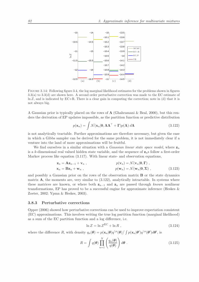
82 3. Approximate inference for multivariate mixtures

−12.5

−12

−11.5

−11

−10.5

−10

(a)

lnZ

−16.5

−16

−15.5

−15

−14.5

−14

(b)−11

−10.9

−10.8

−10.7

−10.6

−10.5

−10.4

−10.3

−10.2

−10.1

−10

(c)−14.5

−14.4

−14.3

−14.2

−14.1

−14

−13.9

−13.8

−13.7

−13.6

−13.5

(d)

MCMC

EC+R

EC/P

VB

Figure 3.14: Following figure 3.4, the log marginal likelihood estimates for the problems shown in figures3.3(a) to 3.3(d) are shown here. A second order perturbative correction was made to the EC estimate oflnZ, and is indicated by EC+R. There is a clear gain in computing the correction; note in (d) that it isnot always big.

A Gaussian prior is typically placed on the rows of Λ (Ghahramani & Beal, 2000), but this ren-ders the derivation of EP updates impossible, as the partition function or predictive distribution

p(xn) =

∫

N (xn|0,ΛΛ⊤ + Γ)p(Λ) dΛ (3.122)

is not analytically tractable. Further approximations are therefore necessary, but given the easein which a Gibbs sampler can be derived for the same problem, it is not immediately clear if aventure into the land of more approximations will be fruitful.

We find ourselves in a similar situation with a Gaussian linear state space model, where zn

is a k-dimensional real valued hidden state variable, and the sequence of zns follow a first-orderMarkov process like equation (3.117). With linear state- and observation equations,

zn = Azn−1 + vn , p(vn) = N (vn|0,Γ) ,

xn = Bzn + wn , p(wn) = N (wn|0,Σ) , (3.123)

and possibly a Gaussian prior on the rows of the observation matrix B or the state dynamicsmatrix A, the moments are, very similar to (3.122), analytically intractable. In systems wherethese matrices are known, or where both zn−1 and zn are passed through known nonlineartransformations, EP has proved to be a successful engine for approximate inference (Heskes &Zoeter, 2002; Ypma & Heskes, 2003).

3.8.3 Perturbative corrections

Opper (2006) showed how perturbative corrections can be used to improve expectation consistent(EC) approximations. This involves writing the true log partition function (marginal likelihood)as a sum of the EC partition function and a log difference, i.e.

lnZ = lnZEC + lnR , (3.124)

where the difference R, with density qn(θ) = p(xn|θ)q\n(θ)/ ∫

p(xn|θ′)q\n(θ′)dθ′, is

R =

∫

q(θ)N∏

n=1

(

qn(θ)

q(θ)

)

dθ . (3.125)

3.8. Summary and outlook 83

The difference can be expanded as a series of small parameters, e.g. ǫn(θ) = 1 − qn(θ)/q(θ).We therefore have a product

∏

n(1 − ǫn(θ)) in equation (3.125); when this is expanded we candrop higher order terms and compute a tractable correction.

The expansion can be computed up to any order for the mixture model examined in thisthesis. We do not present the full derivation and justification here, but show in figure 3.14 thesecond-order corrections for figure 3.4. The corrections to EC give better log evidence estimatesthan both EC/P and VB. This is without doubt an exciting area of research to pursue.

Chapter 4

Parallel Tempering

4.1 Introduction

Parallel tempering, or replica exchange, is an efficient method of combining separate MonteCarlo simulations to sample across different modes of a target distribution. As a by-product thenormalizing constant of the distribution can also be estimated.

This simulation technique has independently been rediscovered in the 1990s by differentauthors, and has consequently been referred to by a number of names: the exchange MC-algorithm, the Metropolis-coupled chain algorithm, time-homogeneous parallel annealing, andthe multiple Markov chain algorithm (Ferkinghoff-Borg, 2002). Its origins can be traced back tothe work of Swendsen & Wang (1986), where a method was introduced where replicas of a systemof interest were simulated at a series of temperatures, and replicas at adjacent temperaturesallowed to exchange partial configuration information. We can also consider parallel temperingas a descendant of the simulated annealing algorithm. Annealing here means that the searchfor the minimum of some function is conducted from a high to a low temperature, with atemperature parameter gradually being decreased to zero. The use of parallel tempering wasinitially restricted to problems in statistical physics, but has since found its way into many fields.For an overview of diverse applications of parallel tempering to polymeric systems, proteins andbiological molecules, crystalline structures, spin glasses and quantum level systems, see (Earl &Deem, 2005).

4.1.1 Replicas at temperatures

A single Markov chain Monte Carlo simulation may run into difficulties if the target distributionis multi-modal. The chain may get stuck in a local mode, and fail to fully explore other areas ofparameter space that have significant probability. One conceptual solution to this problem is tocreate a series of progressively flatter distributions using some temperature parameter. Systemsat higher temperatures, with flatter distributions, should be able to sample from a greater rangeof parameter space. At lower temperature systems may have precise sampling in local rangesof parameter space, but may become trapped in modes that are difficult to escape from withinthe run time taken by a typical simulation. We include a temperature parameter through itsinverse β, where β ranges from zero to one. With the inverse temperature set to one we canwrite the posterior distribution—implicitly giving modelM, of course—in the usual way,

p(θ|x, β) =1

Z(β)p(x|θ)βp(θ) , (4.1)

86 4. Parallel Tempering

where the partition function is

Z(β) =

∫

p(x|θ)βp(θ) dθ . (4.2)

The prior is recaptured with an infinite temperature β = 0, and the log marginal likelihood thatwe are interested in is given by p(x) = Z(1). If the likelihood is flattened with β, the data iseffectively gradually introduced from complete absence at β = 0, to complete presence at β = 1.The correspondence between (4.1) and a Gibbs distribution comes from defining an ‘energy’ asE(θ) = − ln p(x|θ), and then

p(θ|x, β) =1

Z(β)exp

{− βE(θ)

}p(θ) and Z(β) =

∫

exp{− βE(θ)

}dp(θ) . (4.3)

We now simulate K replicas of the original system of interest (4.1), each at a differenttemperature. A set of reciprocal temperatures {βk}Kk=1 are chosen, and we let the set be orderedas a ladder of increasing inverse temperature distributions with βk < βk+1. Here we chooseβ1 = 0, corresponding to the prior, and βK = 1, corresponding to the posterior distribution.

As the simulation of K replicas instead of just one requires K times the computational effort,there must be some solid reasoning for expending this effort. Firstly, an estimate of the marginallikelihood Z(1) can be found. Secondly, it has been observed in practice that a parallel temperingsimulation is more than 1/K times more efficient than a standard, single-temperature MonteCarlo simulation (Earl & Deem, 2005). This is because the replicas allow sampling from lowtemperature systems, for example the true posterior with β = 1, to reach regions of parameterspace that would not otherwise have been practically accessible had we run a single chain atβ = 1 for K times as long.

The key to parallel tempering is that chains at different temperatures are allowed to exchangecomplete configurations or states. Through these exchanges low temperature systems accessdifferent modes or regions of parameter space via the higher temperature systems.

4.1.2 Extended ensembles and replica exchange

As multiple copies of the simulation are run in parallel, each at different temperatures, we there-fore have an extended ensemble, where the parameter space is replicated K times to {θk}Kk=1.With β ∈ {βk}Kk=1 we run K systems in parallel, and the full target distribution that is beingsampled from is

p({θk}Kk=1) =K∏

k=1

1

Z(βk)exp

{

βk ln p(x|θk)}

p(θk) . (4.4)

We run the K chains independently to sample from distributions p(θ|x, βk), and add an addi-tional Metropolis Hastings move to swap two βs between chains, or equivalently swap parametersbetween chains. This is the replica-exchange move. Parallel tempering can be done complemen-tary to any Monte Carlo method at a single temperature, as long as the exchanges satisfydetailed balance. Having chosen two chains i and j for which we want to swap parameters, let{θk}new be the parameter set with parameters θi and θj swapped. The acceptance probabilityfor the move is

α({θk}new|{θk}) = min

(

1,p({θk}new)

p({θk})

)

. (4.5)

4.1. Introduction 87

150 200 250 300 3500

0.02

0.04

0.06

0.08

0.1

0.12

0.14

E(θ)

p(E

)

β = 1β = 0.83β = 0.7β = 0.58β = 0.34β = 0.2β = 0.08β = 0.03− ln p(x)

(a) The distribution of E(θ) = − ln p(x|θ) under replicas at dif-ferent temperatures, p(θ|x, β). These distributions correspond to‘energy histograms’, and following (4.7) there should be an overlapbetween adjacent replicas at different temperatures, so that accep-tance of configuration or parameter swaps is allowed for. For inter-est, the negative log marginal likelihood − ln p(x) is also indicatedon the plot.

0 0.2 0.4 0.6 0.8 1

101

102

103

β

σβ

(b) The standard deviation σβ, from(4.9), as a function of β.

Figure 4.1: These plots show a selection of reciprocal temperatures for the galaxy data set with J = 3components, a prior v0j = 0.01, and all other prior parameters following section 3.7. The averages〈ln p(x|θ)〉βk

for this particular problem and temperature set is illustrated in figure 4.2(a).

As the prior distributions cancel, the ratio between the distributions is

p({θk}new)

p({θk})=

exp{∑k 6=i,j βk ln p(x|θk) + βi ln p(x|θj) + βj ln p(x|θi)}exp{∑k 6=i,j βk ln p(x|θk) + βi ln p(x|θi) + βj ln p(x|θj)}

, (4.6)

which simplifies as

p({θk}new)

p({θk})= exp

{

(βi − βj)(ln p(x|θj)− ln p(x|θi)

)}

. (4.7)

To fully satisfy detailed balance, the swap moves must be performed with a certain probability.Equally, swap moves can be proposed after a fixed number of single temperature Monte Carlomoves. The temperatures of the two replica i and j have to be close to each other to ensurenon-negligible acceptance rates, and in practice only neighbouring temperature pairs are takenas candidates for replica exchanges. For detailed balance a pair {k, k + 1} can be chosen byuniformly choosing a k from between 1 and K − 1.

With this formulation the states of the replicas are effectively propagated from high to lowertemperatures, and the mixing of the Markov chain is facilitated by the fast relaxation at highertemperatures.

4.1.3 Choosing a temperature set

A good choice of {βk}Kk=1 is according to a geometric progression, which we first motivateintuitively. Consider a replica exchange between chains k and k + 1. From equation (4.7), theacceptance probability depends on the difference between ln p(x|θk) and ln p(x|θk+1), and for

88 4. Parallel Tempering

some swaps to be accepted this difference should not be ‘too big’. For a simulation at in inversetemperature β, define the mean evaluation of the log likelihood as

⟨ln p(x|θ)

⟩

β=

∫

ln p(x|θ)p(θ|x, β) dθ . (4.8)

The entire distribution of ln p(x|θ) needs to be considered, and there should be an overlap ofsome of the log likelihood evaluations given by samples for adjacent chains, as shown by figure4.1. The distribution of − ln p(x|θ) under different temperatures is shown in figure 4.1, and weconsider the distribution of the negative log likelihood evaluations for an analogy with an energyfunction in a Gibbs distribution. The variance in chain β is

σ2β = var[ln p(x|θ)]β =

⟨[ln p(x|θ)]2

⟩

β−⟨ln p(x|θ)

⟩2

β, (4.9)

and for the distributions between adjacent temperatures to have a ‘meaningful’ overlap, Iba(2001) has shown that the temperature points should be chosen according to the density

Q(β) ∝ σβ . (4.10)

We give (4.10) in the simplest form amenable to applications in Bayesian inference; in (Ferkinghoff-Borg, 2002) and (Iba, 2001) this density is given in terms of the heat capacity, which also includesthe system size. The following thought experiment should motivate an increase in replicas as thesystem size increases: it may be noted that with more data the likelihoods become increasinglypeaked, and the ‘energy’ distributions become narrower and farther apart, and may lose theiroverlap. The number of replicas needed should therefore increase, at rate O(

√N), with the data

set size N (the width of the distributions of energies sampled increases as the square root of thesystem size).

An obvious difficulty arises, as the variance of the log likelihood as a function of β is notknown in advance, and must be estimated. The minimum required number K and the distribu-tion of temperatures can therefore not be known a priori.

In practice a set of temperatures {βk}Kk=1 can be chosen according to a geometric series,and the average acceptance rate tracked over a short simulation. A rough plot of the estimatedlog likelihood averages and distributions can also give intuition on whether the chain will mixwell over replicas. From (4.10), a larger number of replicas is needed in the region where thevariance of the energy σ2

β takes larger values. Kofke (2002) notes that if the heat capacity isassumed to be constant, the average acceptance probability of a swap depends on temperaturesonly through their ratio, and that a geometric progression with βk/βk+1 = const across alltemperatures should result in equal acceptance ratios (see also (Kofke, 2004)).

4.2 Thermodynamic integration and the marginal likelihood

The samples from parallel tempering can be used for model comparison (Gregory, 2005; Skilling,1998), as the marginal likelihood can be obtained from tempering. Firstly, notice that theintegral

∫ 1

0d lnZ(β) =

∫ 1

0

d lnZ(β)

dβdβ = lnZ(1)− lnZ(0) = lnZ(1) = ln p(x) (4.11)

is equal to the marginal likelihood, as β = 0 gives the prior, which integrates to one. Wetherefore have to determine the derivative d

dβ lnZ(β), and it evaluates as an average over theposterior. Recall that

Z(β) =

∫

p(x|θ)βp(θ) dθ . (4.12)

4.2. Thermodynamic integration and the marginal likelihood 89

By taking the derivative of the log of the partition function,

d lnZ(β)

dβ=

1

Z(β)

∫

ln p(x|θ)× p(x|θ)βp(θ) dθ

=

∫

ln p(x|θ)p(θ|x, β) dθ =⟨ln p(x|θ)

⟩

β, (4.13)

the log marginal likelihood can be evaluated with

ln p(x) =

∫ 1

0

⟨ln p(x|θ)

⟩

βdβ . (4.14)

The integral in (4.14) can be numerically estimated from the Markov chain samples. Let {θ(t)k }

represent the samples for tempering parameter βk, so that the expectation is approximated with

⟨ln p(x|θ)

⟩

βk≈ 1

T

T∑

t=1

ln p(x|θ(t)k ) . (4.15)

We assume that a burn-in sample has been discarded in the sum over t. As we have run a setof chains in parallel at different inverse temperatures 0 = β1 < · · · < βK = 1, the integral canbe evaluated numerically by interpolating the K expectations between zero and one (say with apiecewise cubic Hermite interpolation, available as part of matlab and other standard softwarepackages), and using for example the trapesium rule to obtain the desired result.

4.2.1 The correct interpolation, or glitches at β ≈ 0

To find a numeric approximation to (4.14), a set of log likelihood estimates are interpolated. Inpractice it may happen that we mark a huge factor of difference between the expectations at β1

and β21. As an example, for the galaxy data set (with v0j = 0.01 and J = 3 components) in

sections 3.7 and 4.4.1, β1 = 0 and β2 = 0.001 gave log likelihood averages of −1.72 × 105 and−1.71 × 103 respectively—roughly a difference of a factor of a hundred for a very small changein β.2 If the variance of the prior is increased to v0j = 10−6, this factor grows to roughly 300,giving a large average slope of 3× 105 between 〈ln p(x|θ)〉β=0 and 〈ln p(x|θ)〉β=0.001. Figure 4.3shows the latter log likelihood estimations.

This will differ from problem to problem, and at β = 0 it depends on how likely the data isunder the prior. In this case the log likelihood averages close to zero plays a crucial role in theintegral evaluation, as the tail close to zero can grow like −1/β, which has an infinite integralbetween zero and one.

This problem can be either addressed by simulating at a much finer grid of temperatures inthis interval, or by interpolating the tail with a guess of the exact functional form. The solutionproposed here to interpolating correctly between zero and β2 is to define a function of the form

f(β) = − 1

aβ + b+ c , (4.16)

1The term ‘glitches at β ≈ 0’ is taken from a talk by David MacKay, presented at a Recent Advances in Monte

Carlo Based Inference workshop at the Isaac Newton Institute, Cambridge, 2006.2With Gibbs sampling, described in section 4.4.1, the averages were determined from 9000 samples, after a

1000 sample burn-in. With Gibbs sampling the averages 〈ln p(x|θ)〉β are determined over latent variables z aswell. For brevity here we assume θ includes these extra variables that are averaged over.

90 4. Parallel Tempering

0 0.2 0.4 0.6 0.8 1−500

−450

−400

−350

−300

−250

−200

−150

β

⟨

lnp(x|θ)

⟩

β

(a) The estimate log likelihood averages 〈ln p(x|θ)〉β asa function of β. The values in this plot correspond tothe (negative) means of the energy distributions fromfigure 4.1(a), i.e. −〈E(θ)〉β as temperature 1/β de-creases.

0 0.002 0.004 0.006 0.008 0.01−2

−1.8

−1.6

−1.4

−1.2

−1

−0.8

−0.6

−0.4

−0.2

0x 10

4

β

⟨

lnp(x|θ)

⟩

β

(b) A zoom for β ≈ 0, showing the need for a care-ful interpolation. 〈ln p(x|θ)〉β=0 is approximated as

−1.72 × 105 (the intercept is outside the scale of theplot), while the same expectation at β = 0.001 isroughly a factor of a hundred bigger at −1.71 × 103.

Figure 4.2: The log likelihood averages 〈ln p(x|θ)〉βkare estimated from each of the MCMC simulations

at temperatures {βk}Kk=1, and interpolated so that the integral (4.14) can be evaluated numerically. Inthe problems (see section 4.5) evaluated here, the tail of the interpolation at β ≈ 0 can have a markeddifference in the evaluation of the integral, as it grows like −1/β. A good interpolation can be found withan increasingly fine temperature ladder close to zero. The alternative solution proposed here considersinterpolating the tail with a 1/β-like function. The specific problem illustrated here is again the galaxydata set, with J = 3 components, and v0j = 0.01, and all other prior values set as usual.

0 0.01 0.02 0.03 0.04 0.05−4000

−3000

−2000

−1000

0

β

⟨

lnp(x|θ

)⟩

β

Figure 4.3: Motivation for using (4.16) to determine the value of the integral in (4.14) between β0 = 0and β1. An interpolation with f(β) from (4.16) is shown, passing through β1, β2, and a small βk. Thevalue β1 ≈ −4 × 10−7 is outside the range of the figure. The interpolation is only used to evaluate theintegral between β1 = 0 and β2. The rest of the integral is determined numerically from a piecewise cubicHermite interpolation and trapezium rule. The specific problem illustrated here is again the galaxy dataset, with J = 3 components, and v0j = 10−6, and all other prior values set as usual.

4.3. A practical generalization of parallel tempering 91

and take three values to define the interpolation, β1 = 0, β2, and a βk close to zero. Let thecorresponding log likelihood expectations be L1, L2 and Lk. The coefficients are found by takingthe log likelihood average of chain βk an initial value for c, and then repeatedly solving

a =( 1

c− L1− 1

c− L2

)/

(β1 − β2) , (4.17)

b =1

c− L2− aβ2 , (4.18)

and c = Lk +1

aβk + b. (4.19)

With β1 = 0 and βK = 1, integral (4.14) can in practice be written as

ln p(x) =

∫ β2

β1

⟨ln p(x|θ)

⟩

βdβ +

∫ βK

β2

⟨ln p(x|θ)

⟩

βdβ

≈∫ β2

β1

f(β) dβ +

∫ βK

β2

⟨ln p(x|θ)

⟩

βdβ

=1

a

(

ln(aβ1 + b)− ln(aβ2 + b))

+ c(β2 − β1) +

∫ βK

β2

⟨ln p(x|θ)

⟩

βdβ . (4.20)

The second integral does not include averages around zero, and lends itself to a numericallystable solution.

4.3 A practical generalization of parallel tempering

The success of the interpolation obtaining 〈log p(x|θ)〉β, illustrated in figure 2, is dependent onthe slope

d〈log p(x|θ)〉βdβ

=d2 logZ(β)

dβ2= σ2

β (4.21)

at β ≈ 0. Consider the following thought exercise: Imagine a non-informative (infinitely wide)prior at β = 0. Samples from this prior will strictly speaking have an infinite variance σ2

0 . Withβ ≈ 0 we introduce the likelihood, practically infinitely decreasing the variance of our samples,causing 〈log p(x|θ)〉β to asymptotically diverge at zero. As we narrow our prior the change inthis mean should be less rapid, and this motivates a generalization of parallel tempering andthermodynamic integration such that we get a more stable interpolation.

An ingenious idea proposed by Winther (2007) is to introduce a new distribution q(θ), whichmight be a narrower version of the prior, so that equation (4.1) can be modified to

p(θ|x, β) =1

Z(β)

[

p(x|θ)p(θ)

q(θ)

]β

q(θ) . (4.22)

At β = 0 we are therefore substituting the prior with q(θ). As our ‘effective prior’ is p(θ)βq(θ)1−β ,the prior’s influence is gradually increased, while q’s role is decreased until only the posteriorremains at β = 1. With an informed choice of q, which should be closer than the prior to the trueposterior, we hope to decrease σ2

β. The log marginal likelihood can, as before, be determinedwith

ln p(x) =

∫ 1

0

⟨

ln p(x|θ) + lnp(θ)

q(θ)

⟩

β

dβ . (4.23)

92 4. Parallel Tempering

It does not escape our attention that setting q(θ) = p(θ|x) gives ln p(x) =∫ 10 〈ln p(x)〉β dβ.

This suggests a wealth of possibilities of approximating p(θ|x) with q(θ) to effectively combinedeterministic methods of inference with Markov chains. This comes with a cautionary noteas Variational Bayes, for example, may give a q(θ) that captures (lower-bounds) a mode of apossibly multimodal posterior, causing PT to lose its pleasing property of fast relaxation at hightemperatures. In the results presented in section 3.7, setting q to a narrower version of the prior,where necessary, was found to give adequate results.

In section 4.4.2 a short generalization is given to sample from (4.22) for the mixture ofGaussians problem.

4.4 Gibbs sampling for parallel tempering

Parallel tempering of a mixure of Gaussian distributions p(xn|µ,Λ,π) =∑J

j=1 πjN (xn|µj ,Λ−1j )

require a Monte Carlo simulation at inverse temperature β. As the results obtained here com-plements that of chapter 3, let the mixing weights and component priors again be Dirichlet andNormal-Wishart, with

p(π) = D(π|δ0) =Γ(∑J

j=1 δ0j)∏

j Γ(δ0j)

∏

j

πδ0j−1j (4.24)

p(µ,Λ) =

J∏

j=1

N(µj |m0j , (v0jΛj)

−1)W(Λj |a0j ,B0j) , (4.25)

where

N(µj |m0j , (v0jΛj)

−1)

=(v0j

2π

) d2 |Λj |

12 exp

{

− 1

2tr[(µj −m0j)(µj −m0j)

⊤v0jΛj]}

(4.26)

W(Λj |a0j ,B0j) =|B0j |a0j

∏di=1 Γ(aj + 1−i

2 )π

−d(d−1)4 |Λj |a0j− d+1

2 exp{

− tr[B0jΛj ]}

. (4.27)

In the following two sections describe an implementation of Gibbs sampling to sample from firstlyp(θ|x, β) ∝ p(x|θ)βp(θ), and then from the tempered posterior p(θ|x, β) ∝ p(x|θ)βp(θ)βq(θ)1−β

needed for the generalized version of parallel tempering.

4.4.1 Gibbs sampling at β

To implement a Gibbs sampler, we extend the parameter space to include latent allocationvariables zn for each data point n, to indicate which mixture component was responsible forgenerating it (Diebolt & Robert, 1994). Consequently znj ∈ {0, 1}, and

∑Jj=1 znj = 1. The

complete joint distribution is therefore

p(x, z|θ)p(θ) =N∏

n=1

J∏

j=1

[

πjN (xn|µj ,Λ−1j )]znj

p(θ) , (4.28)

where θ = {π,µ,Λ}. We can write the complete data likelihood as p(x, z|θ) = p(x|θ, z)p(z|θ),and in this form the likelihood, to the power β, is

p(x|θ, z)β =N∏

n=1

J∏

j=1

N (xn|µj ,Λ−1j )βznj (4.29)

4.4. Gibbs sampling for parallel tempering 93

with the prior over θ, z being

p(θ, z) =N∏

n=1

J∏

j=1

πznj

j p(θ) . (4.30)

With inverse temperature parameter β the tempered posterior distribution is

p(θ, z|x, β) ∝ p(x|θ, z)βp(θ, z) =

N∏

n=1

J∏

j=1

N (xn|µj ,Λ−1j )βznjπ

znj

j p(θ) , (4.31)

and can be treated as any missing-value Gibbs sampling problem. The allocation variables aresampled with

znj |π,µ,Λ ∼πjN (xn|µj ,Λ

−1j )β

∑Jk=1 πkN (xn|µk,Λ

−1k )β

. (4.32)

Given the allocation variables, we define

γnj = βznj xj =1

Nj

N∑

n=1

γnjxn

Nj =

N∑

n=1

γnj Σj =1

Nj

N∑

n=1

γnj(xn − xj)(xn − xj)⊤ . (4.33)

to give the conditional distributions needed for sampling the mixture parameters as

π|z ∼ D(δ01 +

1

βN1, . . . , δ0J +

1

βNJ

)(4.34)

µj ,Λj |z ∼ NW(vj,mj , aj ,Bj

), (4.35)

with

vj = v0j +Nj (4.36)

mj =v0jm0j +Njxj

v0j +Nj(4.37)

aj = a0j +Nj

2(4.38)

Bj = B0j +1

2NjΣj +

1

2

Njv0j(xj −m0j)(xj −m0j)⊤

v0j +Nj. (4.39)

As p(x) =∫p(x,θ, z) dθdz, we use the samples over θ and z to estimate the average log

likelihood. If {π(t)k , {µ(t)

j,k,Λ(t)j,k}Jj=1, {z

(t)n,k}Nn=1}Tt=1 indicates the samples of chain k (after a burn-

in period), then

⟨ln p(x|θ, z)

⟩

βk≈ 1

T

T∑

t=1

N∑

n=1

J∑

j=1

z(t)nj,k lnN

(xn|µ(t)

j,k,Λ(t)j,k

−1). (4.40)

Notice that the samples of the mixing weights π(t)k are not used in estimating the log likelihood

average over the posterior, but occur in the prior.

94 4. Parallel Tempering

Algorithm 2 Parallel tempering

1: initialize: π(0)k and {µ(0)

j,k ,Λ(0)j,k}Jj=1 for all chains k; tempering sequence {βk}Kk=1 according

to section 4.1.3; t = 0.2: repeat3: for k = 1 to K do4: for n = 1 to N do5: sample z

(t+1)n,k |π

(t)k , {µ(t)

j,k,Λ(t)j,k}Jj=1 according to (4.32).

6: end for7: sample π

(t+1)k |z(t+1)

k according to (4.34).8: for j = 1 to J do

9: sample µ(t+1)j,k ,Λ

(t+1)j,k |z(t+1)

k according to (4.35).10: end for11: end for12: uniformly choose a chain i ∈ {1, . . . ,K − 1}.13: sample a uniform random variable u ∼ U(0, 1) .

14: if u ≤ α({θnewk }|{θ(t+1)

k }) (see (4.5)) then

15: swap {z(t+1)i ,θ

(t+1)i } and {z(t+1)

i+1 ,θ(t+1)i+1 }

16: end if17: t← t+ 118: until t = tmax

19: for k = 1 to K do20: estimate

⟨ln p(x|θ, z)

⟩

βkwith (4.40), using samples after some burn-in period (this step

can be included in the main loop over t).21: end for22: interpolate {

⟨ln p(x|θ, z)

⟩

βk}Kk=1 between 0 and 1, possibly following section 4.2.1.

23: numerically estimate ln p(x) as the volume under the interpolation.

4.4.2 Gibbs sampling at β for generalized parallel tempering

We have a prior distribution p(θ) = p(π)∏J

j=1 p(µj ,Λj), and to implement a Gibbs sampler forgeneralized parallel tempering, we choose q(θ) to be of the same form as the prior. As in (4.30),both the prior and q(θ) are extended to include latent allocation variables z. The temperedposterior distribution is

p(θ, z|x, β) =1

Z(β)

[

p(x|θ, z)p(θ, z)q(θ, z)

]βq(θ, z)

∝N∏

n=1

J∏

j=1

[

N (xn|µj ,Λ−1j )znj

πznj

j

πznj

j

p(θ)

q(θ)

]β× πznj

j q(θ)

=

N∏

n=1

J∏

j=1

N (xn|µj ,Λ−1j )βznjπ

znj

j p(θ)βq(θ)1−β . (4.41)

The tempered posterior can be factorized into a ‘likelihood’ and a prior:

p(θ, z|x, β) =1

Z(β)

[ N∏

n=1

J∏

j=1

N (xn|µj ,Λ−1j )znj

p(π)p(µ,Λ)

q(π)q(µ,Λ)

]β

4.5. Experimental results 95

×N∏

n=1

J∏

j=1

πznj

j q(π)q(µ,Λ) . (4.42)

To implement a Gibbs sampling as before, we have to determine the parameters of the ‘effective’prior p(θ, z)βq(θ, z)1−β . To differentiate between the parameters of p and q, superscripts p andq will be used. The ‘prior’ parameters, to be used in equations (4.34) to (4.39), are

δ0 = βδp0 + (1− β)δq

0 (4.43)

v0j = βvp0j + (1− β)vq

0j (4.44)

m0j =βvp

0jmp0j + (1− β)vq

0jmq0j

βvp0j + (1− β)vq

0j

(4.45)

a0j = βap0j + (1− β)aq

0j (4.46)

B0j = βBp0j + (1− β)Bq

0j (4.47)

+1

2

βvp0j(1− β)vq

0j

βvp0j + (1− β)vq

0j

(mp0j −mq

0j)(mp0j −mq

0j)⊤ . (4.48)

The empirical expectation given in (4.40) should be generalized to

⟨

ln p(x|θ, z) + lnp(θ)

q(θ)

⟩

βk

≈ 1

T

T∑

t=1

[

ln p(π(t)k )− ln q(π

(t)k ) +

J∑

j=1

[

ln p(µ(t)j,k,Λ

(t)j,k)

− ln q(µ(t)j,k,Λ

(t)j,k) +

N∑

n=1

z(t)nj,k lnN

(xn|µ(t)

j,k,Λ(t)j,k

−1)]]

. (4.49)

4.5 Experimental results

For a practical evaluation of tempered Gibbs sampling, the reader is asked to return to section3.7, where the marginal likelihoods of parallel tempering was compared to that of differentdeterministic methods. This section gives the details of the method in algorithm 2, togetherwith a discussion on some practicalities.

The parameter values were initialized by randomly drawing π(0)k from the prior p(π) for each

chain k. To initialize the means, a k-means algorithm was run for each chain k, and the means

found assigned to the means in the set {µ(0)j,k}Jj=1. The ordering of the assignment of means is

random, and hence different chains should start in different areas of the parameter space, ordifferent modes (we want the chains to be in different modes for good mixing, as we want all

modes to be equally visited). The precision matrices {Λ(0)j,k}Jj=1 were all initialized to the inverse

covariance matrix of the entire data set.

One of the biggest difficulties encountered was to reasonably interpolate 〈ln p(x|θ)〉β aroundβ ≈ 0. For the broad prior used in the experimental section 3.7, there is a factor of around300 difference between β1 = 0 and β2 = 0.001. This gives an average slope of ∆〈ln p(x|θ)〉βas 300,000 for β close to zero. This slope is dependent on the prior width, and decreases asthe prior gets narrower. The final estimate to ln p(x) is very sensitive to the numerical methodaround zero and form of interpolation used to evaluate the integral; where MCMC in section3.7 gives less desirable results, this is usually the cause, and not the chain not mixing well.

96 4. Parallel Tempering

4.6 Discussion: annealed importance sampling

Annealed importance sampling (AIS) (Neal, 2001) is a method closely related to PT. It waspreviously used by Beal & Ghahramani (2003) in a very similar context as section 3.7, namelyas a sampling standard in scoring different marginal likelihood likelihood approximations. Wetherefore aim to present a brief overview, following the introduction given in section 1.3.2. If weare presented with a sample {θ(t)}Tt=1 from some distribution with at least the same support asthe posterior, with associated importance weights {ω(t)}Tt=1, we can approximate the expectedvalue of a function with

〈φ(θ)〉 =∫

φ(θ)p(θ|x) dθ ≈∑T

t=1 ω(t)φ(θ(t))

∑Tt=1 ω

(t). (4.50)

The accuracy of this estimate depends on the variability of the importance weights, and for themethod to work well, we are faced with the difficult task of finding an importance samplingdistribution that approximates the posterior well. (See section 5.4.2 for a practical discussion.)

AIS works by constructing a series of distributions that progressively approximates the pos-terior well. As in PT, we create a series of distributions p(θ|x, β), which we only need to knowup to a normalizing constant. In this setting we shall call it

p∗β(θ) = p∗(θ|x, β) = p(x|θ)βp(θ) . (4.51)

A temperature ladder {βk}Kk=1, with βk < βk+1, is again constructed. We let β1 = 0 recapturethe prior and βK = 1 recapture the posterior. AIS produces a sample {θ(t)}Tt=1 with associatedimportance weights {ω(t)}Tt=1 as follows: For each distribution k = 2, . . . ,K − 1 at inversetemperature βk (therefore excluding the prior at β1 = 0 and the posterior at βK = 1) we definea transition kernel Kk(θ|θ′). This can be a standard Metropolis-Hastings transition kernel or aGibbs sampling update.

To generate a sample θ(t) and its associated weight ω(t) we first generate a sequence ofpoints, walking down the ladder of distributions from an ‘infinite’ temperature (the prior) tothe posterior:

Generate θ2 from p(θ|x, β1) = p(θ) .

Generate θ3 from K2(θ3|θ2) .

· · ·Generate θK−1 from KK−2(θK−1|θK−2) .

Generate θK from KK−1(θK |θK−1) . (4.52)

Finally set θ(t) = θK , and let its associated weight be

ω(t) =p∗2(θ2)

p∗1(θ2)

p∗3(θ3)

p∗2(θ3)· · · p

∗K−1(θK−1)

p∗K−2(θK−1)

p∗K(θK)

p∗K−1(θK). (4.53)

The marginal likelihood can be estimated from the importance weights, as the average of theweights converges to the ratio of normalizers,

1

T

T∑

t=1

ω(t) →∫p∗K(θ) dθ∫p∗1(θ) dθ

as T →∞ . (4.54)

In a Bayesian setting this ratio will be∫p(x|θ)p(θ)dθ/

∫p(θ)dθ, which is equal to the marginal

likelihood. Here we do not even require that the prior is normalized, as all constant factors willcancel in this ratio. For the marginal likelihood to be correct, though, the likelihood has toinclude constant factors.

4.7. Summary and outlook 97

4.7 Summary and outlook

We have seen how parallel tempering can be an effective tool to both sample from multimodalposterior distributions, and estimate the log marginal likelihood.

4.7.1 Other MCMC schemes

A practical problem arises at near-infinite temperatures, or β ≈ 0, as the log likelihood estimatesgrow rapidly as a function of β. This problem is aggrevated by the fact that we have increasedthe dimensionality that we are averaging over with the inclusion of latent variables. A MHmethod could have been used instead, with

p(θ|x, β) =1

Z(β)p(x|θ)βp(θ) =

1

Z(β)

N∏

n=1

[ J∑

j=1

πjN (xn|µj ,Λ−1j )]βp(θ) , (4.55)

as we do not have to increase the space that we have to average over. However, the β powermakes the problem ideally suited to Gibbs sampling, as we can formulate the problem such thatall the conditional distributions are tractable.

It would have been equally possible to integrate out θ, and sample over p(z|x, β), where MHproposals could be ‘bit flips’ on the discrete indicator vectors {zn}Nn=1. Each zn would still beconstrained to have one non-zero bit, indicating to which of the mixture components an observedxn belong. The density that we would sample from in this case would be

p(z|x, β) =1

Z(β)p(x|z)βp(z)

=1

Z(β)

J∏

j=1

(2π)−dNj/2ZNW

(vj , aj ,Bj)

ZNW

(v0j , a0j ,B0j)×Z

D(δ01 + 1

βN1, . . . , δ0J + 1βNJ)

ZD(δ01, . . . , δ0J )

, (4.56)

where vj , aj and Bj are defined in equations (4.36) to (4.39), with dependance on z throughequation (4.33).

4.7.2 Choices for q(θ)

The choice of surrogate prior q(θ) has an effect on the performance of PT, and was originallyintroduced to reduce σ2

β at small values of β. In section 4.3 we argued that q(θ) should matchthe posterior p(θ|x) as closely as possible.

One choice of q(θ) might be a narrower version of the prior. As the posterior is typicallymultimodal, we have to ensure that in some way all the possible posterior modes are still ‘wellcovered’ by q(θ). We can make an intelligent choice based on knowledge of the scale of the dataset.

Another possibility3 is to take a small subset of data points, and analytically evaluate theposterior using the chosen subset. This can in turn be taken as choice for q(θ). With moredata points included, we can expect better performance of PT. There is a trade-off in includingmore data points into the surrogate prior, though, as the problem’s original difficulty lay in thefact that the number of posterior terms grew as JN . We do not give an explicit derivation ofq(θ) here—it is a mixture of Dirichlet-Normal-Wishart products, which can again be effectivelysampled from using Gibbs sampling and further latent variables. An energy histogram obtainedby this improved scheme is shown in figure 4.4(b).

3Thanks to Zoubin Ghahramani for this idea.

98 4. Parallel Tempering

The energy histograms for PT and generalized PT are shown in figures 4.4(a) and 4.4(b).It is possible to observe phase transitions, with largely disconnected energy densities undervarious inverse temperatures β. In figure 4.4(a) the maximum attainable energy would be thelog maximum likelihood evaluation; notice that this is not true any more with the introductionof a surrogate prior. Notice also the ‘better connection’ between the two energy peaks in figure4.4(b). A further step to achieve better sampling across the energy spectrum is multicanonicalsampling (Berg, 2000). This leaves us with a starting point for venturing into the vast fields ofstatistical physics, in the hope of deriving even better algorithms.

4.7. Summary and outlook 99

−300 −250 −200 −1500

0.05

0.1

0.15

0.2

0.25

pβ

[

lnp(x|θ

)]

ln p(x |θ)

0

0.25

0.5

0.75

1

(a) Energy histograms without the introduction of a surrogate prior.

−400 −350 −300 −250 −200 −150 −1000

0.05

0.1

0.15

0.2

0.25

pβ

[

ln{

p(x|θ

)p(θ

)/q(θ

)}

]

ln{

p(x |θ)p(θ)/q (θ)}

0

0.25

0.5

0.75

1

(b) Energy histograms with the introduction of a surrogate prior q(θ). The surrogate prior was chosen as theanalytic posterior q(θ) = p(θ|xn1

,xn3,xn3

) on seeing three (out of 82) data points.

Figure 4.4: This figure follows figure 4.1(a), which shows an approximation to the distributions ofE(θ) = − ln p(x|θ) under replicas at different temperatures, p(θ|x, β), using the means and standarddeviations from samples obtained from different temperature chains. By rather binning evaluations ofln p(x|θ), or ln{p(x|θ)p(θ)/q(θ)}, we obtain more accurate energy histograms. These plots show theenergy histograms for a selection of reciprocal temperatures β (on a coloured scale) for the galaxy dataset with J = 3 components, a prior v0j = 0.01, and all other prior parameters following section 3.7.

Chapter 5

Variational Transition Kernels

5.1 Introduction

In this chapter, variational methods are incorporated into the design of Markov chain MonteCarlo (MCMC) transition kernels. We introduce a new Monte Carlo algorithm, based on avariational approximation to the transition kernel of a Markov chain that has the parameterposterior as invariant distribution, for performing inference with latent variable models.

The idea of combining variational and Monte Carlo methods is by no means new. A mixtureof two MCMC kernels—a sample from the (static) variational approximation to the posteriormixed with a random-walk Metropolis step—was used by de Freitas et al. (2001). The variationalapproximation is used as proposal distribution so that regions of high probability are efficientlylocated; as the approximation underestimates the true variance, a Metropolis kernel is usedto sample from these regions. Ghahramani & Beal (2000) have previously used a variationalapproximation for mixtures of factor analyzers as the proposal density for an importance sampler.In this chapter the variational proposal is not static but adaptive, as it depends on the previousstate of the chain. This also allows for greater exploration of the parameter space. No iterativemethod is needed to find the optimal variational distribution: a closed-form solution for theoptimal kernel, based on the previous state of the chain, exists. The variational transitionkernel will also allow us to circumvent the explicit latent variable sample that is common toGibbs sampling for latent variable models.

This chapter started out as an attempt at a new idea, which finally proved to be less effectivethan expected. What we will illustrate here are the inherent shortcomings of variational methodsin MCMC, giving further insight into why de Freitas et al. (2001), for example, found it necessaryto mix random-walk steps into their MCMC algorithm. The shortcomings mostly pertain toproblems with the variance of estimates obtained from the samples. (The cause of this behaviorcan be traced back to section 2.2 in chapter 2, where it was illustrated how VB underestimatesthe true variance of the density it approximates.) For Metropolis-Hastings, the resulting chaincannot be shown to be geometrically ergodic, and we cannot show the existence of a centrallimit theorem for our estimate. We will show how importance sampling can suffer from a similarproblem of possibly infinite variance of the importance weights.

The rest of the chapter takes a short theoretical tour through the world of general statespace Markov chains and Monte Carlo integration in section 5.2, presenting some theory neededto show different forms of convergence later in the chapter. The Metropolis Hastings algorithmis introduced as a practical method of constructing a Markov chain with a particular predefineddistribution as its stationary distribution. We then introduce variational methods into MCMCtransition kernels in section 5.3. We give a detailed analysis on a small toy example in section

102 5. Variational Transition Kernels

5.4, to see what the shortcoming of such an approach is.

5.2 Monte Carlo methods

The principle of drawing samples from a distribution, and using sample averages to approximateexpectations, lies at the heart of Monte Carlo integration. This forms a flexible method withgreat scope in statistical modeling. The exposition presented here assumes that some posteriordistribution is the distribution of interest, but the underlying principles can readily be appliedto any distribution.

5.2.1 Monte Carlo integration

Many tasks in Bayesian inference require the evaluation of an expectation of some function,say φ(θ), over a distribution of interest. Our interest generally lies in the posterior distribu-tion p(θ|x,M), for which we implicitly condition on the model assumptions M to write theexpectation as

Φ = 〈φ(θ)〉 =

∫

φ(θ)p(θ|x) dθ . (5.1)

The principle behind Monte Carlo integration is to approximate such an integral with an em-pirical average; if we are able to draw independent and identically distributed samples {θ(t)}Tt=1

from the target distribution p(θ|x), then Φ can be approximated with the unbiased estimate

ΦT =1

T

T∑

t=1

φ(θ(t))→ Φ . (5.2)

By the law of large numbers the estimate will converge almost surely to Φ, P(ΦT = Φ) = 1as T → ∞. Crucially, the variance of the estimate will be well behaved: If the variance ofφ(θ) is finite, σ2

φ ≡ 〈φ2(θ)〉 − 〈φ(θ)〉2 < +∞, then the variance of the estimate is equal to

var(ΦT ) = σ2φ/T , and a central limit theorem yields convergence in distribution of the error√

T (ΦT − Φ) → N (0, σ2φ) as T → ∞ (Andrieu et al., 2003). The central limit theorem result

holds if we are able to draw i.i.d. samples.

It is generally not possible to draw independent samples from p(θ|x). However, the samples{θ(t)} need not be independent, but can loosely speaking be simulated using any process thatdraws samples from the support of p(θ|x) in the correct proportions. One possible such processis a Markov chain that has p(θ|x) as its stationary distribution; the chain can be simulatedand the resulting series of states taken as samples. For brevity, we let p∗(θ) indicate the targetdistribution.

5.2.2 Markov chains

A Markov chain generates a sequence of random variables {θ(0),θ(1), . . .} where the next state ofthe chain θ(t+1) is sampled from a transition kernel K(θ|θ(t))1, a conditional probability densitythat only depends on the current state of the chain. The next state of the chain is thereforeindependent of the history of the chain. Markov chain Monte Carlo methods are constructedfrom a time homogeneous chain, that is, the transition kernel is independent of t.

1Instead of K(θ(t); θ), we use the less common notation K(θ|θ(t)) in the Bayesian sense, as the distribution ofθ(t+1) is conditional on the present value of θ(t).

5.2. Monte Carlo methods 103

The distribution of a time-homogeneous Markov chain {θ(t)} is affected by the transitionkernel and the initial state (or distribution of the initial state). Of key importance is that thedistribution of the sampler’s state converges to the correct invariant distribution, regardless ofthe starting state θ(0). The influence of the starting state θ(0) on θ(t) affects the ergodicityof the chain, and our hope is that the initial state will gradually be forgotten. If the chainis ergodic the invariant distribution should be reachable from any initial distribution. Thedistribution K(t)(θ|θ(0))—the distribution of θ(t) given the starting value θ(0)—should convergeto the stationary distribution as t→∞. The tth iterate of transition kernel is recursively definedas

K(t)(θ|θ(0)) =

∫

K(θ|θ′)K(t−1)(θ′|θ(0)) dθ′ . (5.3)

Under certain regularity conditions the initial state will have no effect on the long-term outcomeof the chain, and K(t)(θ|θ(0)) will converge to a stationary or invariant distribution, independentof the initial state or t. A brief overview of these conditions is given below.

After a period of, say, m samples, the samples {θ(t)}Tt=m+1 will be a set of dependent samplesthat approximately come from the target density. This initial set of samples is called the burn-in,and is usually discarded when estimators are determined, i.e. ΦT = 1

T−m

∑Tt=m+1 φ(θ(t)).

Conditions guaranteeing convergence to a stationary distribution

A few conditions are sufficient to ensure that the distribution of the state of a Markov chainconverges to the invariant distribution. These conditions are needed for the law of large numbersto hold for sample path averages, such that the empirical estimate Φ converges to the trueexpectation Φ. As we will later see with a toy example in section 5.4.1, we may need additionalconditions to ensure a central limit theorem and say something meaningful about the varianceof the estimate.

We first define the ‘distance’ between two probability distributions p1 and p2 with the totalvariation norm,

‖p1 − p2‖ = 2 supA∈Θ|p1(A)− p2(A)| , (5.4)

where we use notation p(A) =∫

A p(θ)dθ. We also need the concept of the first return time of

the Markov chain to set A, indicated by τA, and properly defined as τA = inf{t ≥ 1 : θ(t) ∈ A},with τA =∞ if the chain never returns to A.

For the Markov chain to converge to its stationary distribution the chain must be:

Irreducible. Given any initial state, the chain has to be able to reach any other state with apositive probability in a finite number of steps. For general state-space Markov chains,the definition of irreducibility is with respect to a distribution (Gilks et al., 1996):

Definition 1. A Markov chain is ϕ-irreducible for a probability distribution ϕ on Θ ifϕ(A) > 0 for a set A ⊂ Θ implies that

P(τA <∞ | θ(0)) > 0 (5.5)

for all θ(0) ∈ Θ. A chain is irreducible if it is ϕ-irreducible for some probability distributionϕ. If a chain is ϕ-irreducible, then ϕ is called an irreducibility distribution for the chain.

An irreducible chain has many irreducibility distributions, all of which are absolutelycontinuous with respect to some maximal irreducibility distribution ψ. (Saying that p1 isabsolutely continuous with respect to p2 here means that if p2(A) > 0, then p1(A) > 0, forany A ∈ Θ.)

104 5. Variational Transition Kernels

Aperiodic. The chain must not by cyclic, so that an oscillation between two states, or sets ofstates, is for example not possible.

Recurrent. If a chain is irreducible then all interesting sets can be reached. Recurrence impliesthat all such sets can be reached infinitely often, from all starting positions. A distinctionis made between positive recurrent chains, where the average return time to all states isfinite, and null recurrent chains, where the average time to return to some state can beinfinite. For discrete chains positive recurrence is needed, and follows from the existence ofan invariant distribution. For general state-space chains we have the following definition(Gilks et al., 1996):

Definition 2. An irreducible Markov chain with maximal irreducibility distribution ψ isrecurrent if for any set A ⊂ Θ with ψ(A) > 0

1. P(θ ∈ A infinitely often | θ(0)) > 0 for all θ(0), and

2. P(θ ∈ A infinitely often | θ(0)) = 1 for ψ-almost all θ(0).

An irreducible recurrent chain is positive recurrent if it has an invariant distribution,otherwise it is null recurrent.

As the chain is started from any initial θ(0), we need to be sure that the chain has the samelimiting behaviour for every starting value instead of almost every starting value. This isensured by Harris recurrence, a stronger condition which requires P(θ ∈ A infinitely often| θ(0)) = 1 for all θ(0).

If we can show that the Markov chain {θ(t)} is irreducible and has invariant distribution p∗(θ),then the chain is p∗-irreducible, p∗(θ) is a maximal irreducibility distribution, p∗(θ) is the uniqueinvariant distribution of the chain, and the chain is positive recurrent. Recurrence is sufficientto imply convergence of averages of probabilities, and to let a strong law of large numbers hold(Gilks et al., 1996):

Theorem 3. If {θ(t)} is an irreducible Markov chain with transition kernel K and invariantdistribution p∗, and φ(θ) a real-valued function such that

∫|φ(θ)|p∗(θ) dθ <∞. Then P(ΦT →

Φ | θ(0)) = 1 for p∗-almost all θ(0), where ΦT and Φ are defined in (5.2) and (5.1).

Whether a Markov chain will converge to its invariant distribution is given by the followingresult:

Theorem 4. Suppose {θ(t)} is an irreducible, aperiodic Markov chain with transition kernel Kand invariant distribution p∗. Then

‖K(t)(·|θ)− p∗(·)‖ → 0 (5.6)

for p∗-almost all θ.

This convergence result will hold for all θ if and only if we can guarantee that the chainis positive Harris recurrent as well. (Harris recurrence will hold for the samplers that we areconcerned with in this chaper.) For a positive Harris recurrent chain, asymptotic results, suchas laws of large numbers and central limit theorems, that do not depend on any initial portionof a sample path can be shown to hold for all initial distributions if they hold for any.

5.2. Monte Carlo methods 105

Central Limit Theorems

Thus far we have seen that positive recurrence alone is sufficient to ensure that a law of largenumbers holds for a Markov chain, and hence that ergodic averages converge to their expectationsunder the stationary distribution. Ergodic averages ΦT , and the asymptotic properties of theseaverages, are clearly very important. The ergodic theorem 3 does however not specify (a) howlong we need to run the chain for, and (b) it gives no estimate of the size of error that theestimate ΦT makes.

We need stronger conditions for theorem 4 besides recurrence to provide a central limittheorem. A condition that is often used, also in this chapter, is that of geometric convergencefor ergodic chains, that is, chains that are irreducible, aperiodic and positive Harris recurrent.

Definition 3. An ergodic Markov chain with invariant distribution p∗(θ) is geometrically ergodicif there exists a non-negative extended real-valued function M such that

∫M(θ)p∗(θ) dθ < ∞

and a positive constant r < 1 such that

‖K(t)(·|θ) − p∗(·)‖ ≤M(θ)rt (5.7)

for all θ and all t.

If function M does not depend on θ in the above definition, i.e., it is constant, then thestronger condition gives uniform convergence. Importantly, a Markov chain that is geometricallyor uniformly ergodic satisfies a central limit theorem (Gilks et al., 1996):

Theorem 5. Suppose an ergodic Markov chain {θ(t)} with invariant distribution p∗ and a realvalued function φ satisfy one of the following conditions:

1. The chain is geometrically ergodic and∫|φ(θ)|2+ǫp∗(θ) dθ <∞ for some ǫ < 0.

2. The chain is uniformly ergodic and∫φ(θ)2p∗(θ) dθ <∞.

Then

σ2φ = Ep∗[(φ(θ(0))− Φ)2] + 2

T∑

t=1

Ep∗ [(φ(θ(0))−Φ)(φ(θ(t))− Φ)] (5.8)

is well defined, non-negative and finite, and√T (ΦT −Φ) converges in distribution to a N (0, σ2

φ)random variable.

(In the above theorem the esimator ΦT = 1T+1

∑Tt=0 φ(θ(t)) counts from zero).

The notion of geometric convergence will reoccur in section 5.4.1, when we observe that thevariational kernel, that will later be introduced, gives ‘sticky tails’. Geometric convergence willbe the key to showing that simply sampling with a variational proposal cannot, in a simplecase examined, give a Central Limit Theorem. Before considering variational approximations totransition kernels, a short overview of the Metropolis Hastings algorithm is given.

5.2.3 Metropolis-Hastings

Markov chain Monte Carlo methods are constructed such that the stationary condition of de-tailed balance holds,

p∗(θ(t))K(θ(t+1)|θ(t)) = p∗(θ(t+1))K(θ(t)|θ(t+1)) . (5.9)

As usual we let p∗(θ) be a (possibly unnormalised) shorthand for p(θ|x).

106 5. Variational Transition Kernels

Constructing a Markov chain with p∗(θ) as stationary distribution is very easy with themethod of Metropolis et al. (1953), later generalized by Hastings (1970). At each time t, a newstate θnew is generated from a proposal distribution q(θ|θ(t)). This new state is a candidatethat is being accepted with probability

α(θ(t),θnew) = min

(

1,p∗(θnew)q(θ(t)|θnew)

p∗(θ(t))q(θnew|θ(t))

)

. (5.10)

If the proposed state is accepted the next state in the chain becomes θ(t+1) = θnew, otherwisethe state of the chain does not change with θ(t+1) = θ(t). An overview is given in algorithm 3.

When the support of q includes the support of p∗(θ), the resulting transition kernel

K(θ|θ(t)) = α(θ(t),θ)q(θ|θ(t)) + [1− acc(θ(t))]δ(θ = θ(t)) (5.11)

satisfies the detailed balance condition and the stationary distribution of the chain will be p∗(θ).The transition kernel consists of two terms, the first is the probability of generating a new pointmultiplied by the probability of accepting it, and the second is the probability of repeating theprevious sample θ(t). Notation acc(θ(t)) =

∫α(θ(t),θ)q(θ|θ(t))dθ indicates the probability of

accepting a new point, while δ(· = θ(t)) indicates the Dirac delta mass at θ(t).From (5.10) we have

p∗(θ(t))q(θ(t+1)|θ(t))α(θ(t),θ(t+1)) = p∗(θ(t+1))q(θ(t)|θ(t+1))α(θ(t+1),θ(t)) , (5.12)

from which we obtain the detailed balance equation

p∗(θ(t))K(θ(t+1)|θ(t)) = p∗(θ(t+1))K(θ(t)|θ(t+1)) . (5.13)

When we integrate both sides of this equation with respect to θ(t) we get the stationary distri-bution condition ∫

p∗(θ(t))K(θ(t+1)|θ(t)) dθ(t) = p∗(θ(t+1)) , (5.14)

and K is the correct transition kernel. Therefore, the equation says that if θ(t) comes fromp∗(θ(t)), then θ(t+1) will come from the same stationary distribution. Once we have a samplefrom the stationary distribution, all subsequent samples will also be from that distribution. Tofully justify the MH algorithm we need more than just a stationary distribution, we also needa guarantee that K(t)(θ|θ(0)) will converge to the stationary distribution. From constructionof the MH method, we already have a stationary distribution, while aperiodicity follows fromthe fact that the MH algorithm allows for rejection. Finally, for irreducibility we only need toensure that q(θ|θ(t)) > 0 over the entire space.

Whether the algorithm succeeds in exploring all modes of parameter space often depends onthe choice of proposal distribution. If the proposal is too narrow, the chain may only exploreone mode, while if on the other hand it is too wide, the rejection rate can be very high. We haveseen in chapter 4 how parallel tempering, with fast relaxation at high temperature simulations,can be used to ensure that the chain mixes well and all modes be visited with high acceptanceprobability.

We will now explore a new route, leading from the cross roads of approximate inferencefrom chapters 2 and 3, and MCMC methods discussed earlier in this chapter. In the spiritof variational methods, an approximation to a ‘good’ transition kernel will be made, and adetailed discussion and proof given illustrating why such an approximation may lead to failureof a MCMC method.

5.3. Variational transition kernel 107

Algorithm 3 Metropolis-Hastings

1: initialize: θ(0), t = 0.2: repeat3: sample θnew from q(θ|θ(t)).4: sample a uniform random variable u ∼ U(0, 1) .5: if u ≤ α(θ(t),θnew) then6: set θ(t+1) = θnew

7: else8: set θ(t+1) = θ(t)

9: end if10: t← t+ 111: until t = tmax

5.3 Variational transition kernel

A natural setting for variational transition kernel sampling arises when the posterior can becompleted with latent variables z into a joint distribution p(θ, z|x), such that the completedposterior distribution p(θ|x, z) becomes easy to evaluate (Robert & Casella, 2004).

For completeness the familiar example of chapters 2, 3 and 4 is repeated here. In mixtureof distributions, we assume that the examples in x = {xn}Nn=1 are independent and identicallydrawn from p(xn|θ) =

∑Jj=1 πjp(xn|θj). Let θ encompass all unknown parameters in the model:

the parameters of the J component distributions p(·|θj) and the component weights πj that sumto one. Hidden latent variables z = {znj}, where znj is equal to 1 if xn was generated fromcomponent j in the mixture, and zero otherwise, naturally augment the data. The likelihood,which considers all possible partitions of the sample and expands into JN terms, and the ‘easier’complete-data likelihood are

p(x|θ) =

N∏

n=1

[ J∑

j=1

πjp(xn|θj)]

and p(x, z|θ) =

N∏

n=1

J∏

j=1

[

πjp(xn|θj)]znj

. (5.15)

5.3.1 An exact transition kernel

We can draw samples from the posterior distribution over θ if we can construct a transitionkernel K(θ|θ′) that has the parameter posterior as correct invariant distribution,

∫

K(θ|θ′)p(θ′|x) dθ′ = p(θ|x) , (5.16)

and that marginalizes out the latent variables. Samples from K are then coming from theposterior distribution p(θ|x), and we can create such a sample {θ(t)} by defining K with:

1. Given θ′ (i.e. θ(t−1)), determine p(z|x,θ′).

2. Given p(z|x,θ′), sample θ (i.e. θ(t)) from

K(θ|θ′) =

∫

p(θ|x, z)p(z|x,θ′) dz . (5.17)

108 5. Variational Transition Kernels

This kernel is exact as we can show that p(θ|x) is the invariant distribution with a rearrangement,

∫

K(θ|θ′)p(θ′|x) dθ′ =

∫{∫

p(θ|x, z)p(z|x,θ′) dz

}

p(θ′|x) dθ′

=

∫{∫p(x, z|θ)p(θ)

p(x, z)

p(x, z|θ′)p(x|θ′)

dz

}

p(x|θ′)p(θ′)p(x)

dθ′

=

∫p(x, z|θ)p(θ)

p(x, z)

∫p(x, z|θ′)p(x|θ′)

p(x|θ′)p(θ′)p(x)

dθ′ dz

=1

p(x)

∫

p(x, z|θ)p(θ) dz =p(x|θ)p(θ)

p(x)= p(θ|x) , (5.18)

and therefore if the kernel is used as proposal density in a MH algorithm, the acceptance ratioin (5.10) will always be unity.

This construction is similar to doing Gibbs sampling with z ∼ p(z|x,θ′) and θ ∼ p(θ|x, z).We arrive at an alternative sampling scheme, as choosing K in this way to average over the latentvariable space allows a derivation of a transition kernel that replaces discrete or categorical modelchanges with continuous ones.

5.3.2 A tractable approximation

The required transition kernel is, however, in general not analytically tractable and impossibleto sample from directly. The kernel can be approximated by finding a proposal density q(θ|θ′)that is close to K(θ|θ′) (remembering that sampling with K automatically gives the requiredinvariant distribution and can in theory be used as a proposal density, although in practice it isnot analytically tractable) by minimizing the Kullback-Leibler divergence between the definedproposal and the kernel (exact proposal),

KL(q‖K) =

∫

q(θ|θ′) lnq(θ|θ′)K(θ|θ′)

dθ . (5.19)

The problem that we face is that K is not in a product form (unlike p(θ, z|x), for example).This means that even if a specific factorization of q is assumed, a tractable solution will not befound. However, Jensen’s inequality can be used to construct an upper bound to KL(q‖K), andthis bound can in turn be minimized to give an analytical solution:

lnK(θ|θ′) ≥∫

p(z|x,θ′) ln p(θ|x, z) dz . (5.20)

It is important to note that this is a bound for the distribution in z, so the equality onlyholds in the extreme cases of deterministic relation or independence: p(z|x,θ′) = δ(z − z0) orp(θ|x, z) = p(θ|x). We now have an upper bound:

KL(q‖K) ≤∫

q(θ|θ′)[

ln q(θ|θ′)−∫

p(z|x,θ′) ln p(θ|x, z) dz]

dθ ≡ F [q(θ|θ′)] . (5.21)

The minimum of KL(q‖K), which is q = K, is of course not attained by minimizing the upperbound F (apart from the trivial case discussed above). The solution can, as we see in thefollowing, still serve as a useful approximation to the transition kernel.

5.3. Variational transition kernel 109

The usual free form optimization, typical of variational methods, can be used to find anappropriate q. A Lagrange multiplier ℓ is added to the functional such that q is constrained tointegrate to one, with

F [q(θ|θ′)] = F [q(θ|θ′)] + ℓ[ ∫

q(θ|θ′) dθ − 1]

. (5.22)

By using elementary calculus of variations, we take the functional derivative of F [q] with respectto q under the integral constraint to make q a density,

∂F [q(θ|θ′)]∂q(θ|θ′)

=

∫

p(z|x,θ′)[ ∂

∂q(θ|θ′)

∫

q(θ|θ′) lnp(θ|x, z)q(θ|θ′)

dθ]

dz

· · ·+ ∂

∂q(θ|θ′)ℓ[ ∫

q(θ|θ′) dθ − 1]

(5.23)

=

∫

p(z|x,θ′)[ln p(θ|x, z) − ln q(θ|θ′)− 1] dz + ℓ ,

and set it to zero:

ln q(θ|θ′) =

∫

p(z|x,θ′) ln p(θ|x, z) dz− 1 + ℓ . (5.24)

By exponentiating and integrating over θ on both sides, keeping the integral constraint in mind,we can solve for ℓ to correctly normalize the distribution. The upper bound on the divergenceis therefore minimized with

q(θ|θ′) = exp{∫

p(z|x,θ′) ln p(θ|x, z) dz}/∫

exp{∫

p(z|x,θ′) ln p(θ|x, z) dz}

dθ . (5.25)

Using Bayes’ theorem we get the variational approximation to the transition kernel,

q(θ|θ′) ∝ p(θ) exp{∫

p(z|x,θ′) ln p(x, z|θ) dz}

. (5.26)

This form is instantly recognizable from the Variational Bayesian EM algorithm, as discussedin section 1.4.3.

5.3.3 Illustrative example: Mixture of distributions

As an illustrative example, consider the mixture of distributions discussion from the start ofSection 5.3. Let p(zn|xn,θ

′) = γn = (γn1, . . . , γnJ) be the probability that xn was generatedby each of the J components (the component’s responsibility), thus defining a distribution overeach binary vector zn. Then the responsibilities are

γnj = p(znj = 1|xn,θ′) =

πjp(xn|θ′j)

∑Jk=1 πkp(xn|θ′

k). (5.27)

Using the log of the complete-data likelihood from equation (5.15) and p(z|x,θ′) determinedabove, we get

∑

zln p(x, z|θ)p(z|x,θ′) =

∑Nn=1

∑Jj=1 γnj ln[πjp(xn|θj)], and from equation

(5.26),

q(θ|θ′) ∝ p(θ)J∏

j=1

N∏

n=1

[

πjp(xn|θj)]γnj

. (5.28)

110 5. Variational Transition Kernels

θ

z

−2 −1 0 1 2

−2

−1

0

1

2qθ(θ)q

z(z)

p(θ,z)

−2 −1 0 1 2 θ

p(θ)

qθ(θ)

K(θ|θ’)q(θ|θ’)

θ’

rθ’

Figure 5.1: A toy example of a two-dimensional Gaussian over θ and z, centered at zero, with covariancematrix Σ = [1, 0.98; 0.98, 1]. The variational Bayes approximation qθ(θ)qz(z) to p(θ, z) is shown on theleft. The marginal p(θ) and the factor qθ(θ) from the variational approximation to p(θ, z) is on the right.With θ′ = 1.3, K(θ|θ′) and q(θ|θ′), both with mean rθ′, are also shown. (The densities are not normalisedin the figure.)

The kernel simply raises the likelihood terms to its respective responsibility powers, and if p(·|θj)comes from an exponential family of distributions the result will be a weighted contribution ofdata points to each mixture component. Notice that if γnj is discrete, we fall back directly totwo-stage Gibbs sampling, where a discrete sample znj ∈ {0, 1} is used instead of γnj ∈ [0, 1].Effectively we have replaced categorical labels with continuous variables. When γ is strictlybinary the kernel approximation is of course exact.

A potential difficulty surfacing here is that the true kernel may be multimodal, but weattempt to approximate it with a distribution of single mode, as was seen in examples in chapter2. As is true for variational methods where a factorization qθ(θ)qz(z) is assumed, the varianceof the approximation—similar to the variance of qθ(θ) from a variational lower bound—is anunderestimation of the true variance of the kernel. In approximate methods this is acceptable,but it may be ruinous when we are concerned with creating a practical MCMC method (seesection 5.4.1 for a formal discussion).

5.4 Using the proposal in Monte Carlo methods

Although the main idea of taking a Markov chain with an intractable transition kernel K(θ|θ′)and correct invariant distribution, and approximating K with q(θ|θ′) as a MH proposal, soundsappealing, some questions on convergence can be raised. It turns out that simply using q asproposal is not enough, and the method needs to be supplemented with additional standardmoves (symmetric proposal densities, for instance), or dropped altogether in favour of moreorthodox samplers (the Gibbs sampler of chapter 4 being a good example). The following toyexample is insightful.

5.4.1 Toy example

As an informal illustration to compareK(θ|θ′), the approximation q(θ|θ′) as MH proposal density,and the variational approximation qθ(θ), consider a two-dimensional Gaussian, where ρij indicatethe elements of the inverse covariance matrix,

p(θ, z) ∝ exp{− 1

2 [ρ11θ2 + (ρ12 + ρ21)θz + ρ22z

2]}. (5.29)

5.4. Using the proposal in Monte Carlo methods 111

−3 −2 −1 0 1 2 30

0.9391

θ’

∝ p(θ’)E

q(θ|θ’)[α(θ|θ’)]

Ep(θ’)

[Eq(θ|θ’)

[α(θ|θ’)]]

Figure 5.2: Continuing Figure 5.1’s toy example. The average acceptance probability E[α(θ|θ′)] isshown as a function of θ′. Averaging E[α(θ|θ′)] numerically over p(θ′) gives 0.939 as average acceptanceover the target distribution.

Let

r ≡ (ρ12 + ρ21)2

4ρ11ρ22, (5.30)

with r ∈ [0, 1). The example is chosen such that K(θ|θ′) from (5.17) is analytically tractable,and also such that the required marginal p(θ)—that we would like to draw samples from—canbe analytically normalized. The marginal and conditional distributions for θ are

p(θ) = N(θ∣∣ 0, [ρ11(1− r)]−1

)(5.31)

and p(θ|z) = N(

θ∣∣∣ − (ρ12 + ρ21)

2ρ11z, ρ−1

11

)

. (5.32)

The marginal p(z) and conditional p(z|θ) are the same as above, except that occurrences of ρ11,ρ22 and z are respectively swapped with ρ22, ρ11 and θ. Here both K(θ|θ′) =

∫p(θ|z)p(z|θ′) dz

and the approximation q(θ|θ′) = 1Z exp{ln p(θ|z)p(z|θ′) dz} are analytically tractable,

K(θ|θ′) = N(θ∣∣ rθ′, ρ−1

11 (1 + r))

(5.33)

q(θ|θ′) = N(θ∣∣ rθ′, ρ−1

11

). (5.34)

A further possible approximation to note is that given by Variational Bayes, where p(θ, z) isapproximated with a factorized Gaussian qθ(θ)qz(z), the minimizer of KL(qθ(θ)qz(z) ‖ p(θ, z)).The factor involving θ is

qθ(θ) = N(θ∣∣ 0, ρ−1

11

), (5.35)

which can naively be taken as a proposal density. Figure 5.1 plots all of these densities, showingthat an adaptive proposal q(θ|θ′) appears more sensible (in terms of exploration) than usingqθ(θ) as proposal. The variational (approximate) kernel q(θ|θ′) illustrates the potential under-estimation of the variance of K(θ|θ′): here by a factor of (1 + r). How much the variance isunderestimated depends on the strength of coupling between θ and z, with q = K when r = 0.When the q(θ|θ′) is used as a MH proposal density, E[α(θ|θ′)] is in practice close to one in areasof high density and good approximation (see Figure 5.2 with regard to this example). However,due to the underestimation of the variance by the variational approximation, the variationalproposal may fail to produce adequate results at the tails of a distribution. A similar effectoccurs when the exact kernel is multimodal, and is approximated with a distribution with singlemode. This problem is discussed in more detail in the following section.

112 5. Variational Transition Kernels

0 200 400 600 800 1000−2

0

2

4

6

8

10

12

14

16

18

Time t

θ(t)

Figure 5.3: An illustration of why the approximation q(θ|θ′) may not give a geometrically ergodicchain. Different chains are started further down the tails of the target distribution p(θ), and the averageacceptance probability can be made arbitrarily small by choosing a θ(t) far enough down the tail of thedistribution. In this example the covariance matrix Σ = [1, 0.98; 0.98, 1] was used, giving ρ11 = ρ22 =25.2525 and ρ12 = ρ21 = −24.7475. The standard deviation of the target density p(θ) is 1; the chainswere started at least 10 standard deviations away from p(θ)’s mean.

Geometric ergodicity

To provide for a central limit theorem on the estimate ΦT , i.e. to have√T (ΦT − Φ) converge

in distribution to a Gaussian zero-mean random variable with finite, well-defined variance, acondition on the convergence rate of {θ(t)} is typically needed. An often-considered convergencerate condition is geometric ergodicity.

Continuing the toy example, figure 5.3 illustrates the use of q(θ|θ′) as proposal, with differentchains starting further down the tails of the target distribution p(θ). It will be shown later thatthe tails become ‘sticky’, with arbitrarily small average acceptance probability—this forms thecore of showing that the chain is not geometrically ergodic. Section 5.4.3 presents a simplemethod for addressing this problem.

Preliminary theory

We want to be able to show that a chain is geometrically ergodic, or not, and here only thenecessary theory for the proof is given. For general state-space chains, we need the notion ofa small set. A small set will play a role similar to individual states in a discrete chain, and inmany problems under consideration compact sets are small.

Definition 4. A set C ⊂ Θ is small for an irreducible transition kernel K with maximalirreducibility distribution ψ if ψ(C) > 0 and there exists a probability distribution ν on Θ, anon-negative integer t, and a constant β > 0 such that K(t)(A|θ) ≥ βν(A) for all θ ∈ Θ and allA ⊂ Θ.

The following theorem is adapted from (Mengersen & Tweedie, 1996) and will be used in showinggeometric ergodicity.

Theorem 6. Suppose that {θ(t)} is ϕ-irreducible and aperiodic. Then the following is an equiv-alent definition for a geometrically ergodic chain:

5.4. Using the proposal in Monte Carlo methods 113

• For some small set C with ϕ(C) > 0, there exists a κ > 1 such that

supθ∈C

Eθ[κτC ] = supθ∈C

∞∑

k=0

P[τC ≥ k]κk <∞ . (5.36)

(The notation Eθ indicates the expectation for a Markov chain started in state θ(0) = θ ∈ C.)

We are now in the position to pinpoint where the use of the variational approximation tothe kernel may fail, and the proof merely gives a formal description of figure 5.3.

Proposition 1. Provided that r > 0, the toy example’s proposal density q(θ|θ′) does not giverise to a geometrically ergodic Metropolis Hastings chain.

Proof. Consider some θ′. The acceptance ratio, as a function of θ′, is an exponential that issymmetric around zero, the mean of p(θ),

A = exp{12ρ11r(1− r)(θ2 − θ′2)} , (5.37)

with ρ11r(1−r) being nonnegative. Given θ′, a proposed θ is accepted with probability α(θ′, θ) =min(1, A). The average acceptance probability, as a function of θ′, is

a(θ′) ≡ E[α(θ′, θ)] =

∫

|θ|<|θ′|AN (θ | rθ′, ρ−1

11 ) dθ +

∫

|θ|≥|θ′|1N (θ | rθ′, ρ−1

11 ) dθ , (5.38)

and we can show that it can be made arbitrarily small by choosing θ′ further away from zero.Evaluating a(θ′) for θ′ > 0 gives

a(θ′) =(ρ11

2π

)1/2exp

{

− 1

2ρ11r

(1− r

r2 − r + 1

)θ′2}

· · · ×∫

|θ|<|θ′|exp

{

− 1

2ρ11[r

2 − r + 1](θ − rθ′

r2 − r + 1

)2}

dθ

︸ ︷︷ ︸

≤(2π/ρ11[r2−r+1])1/2

· · ·+ Φ(

− θ′(1 + r)√ρ11

)

+[

1− Φ(

θ′(1− r)√ρ11

)]

, (5.39)

where Φ(·) is the N (0, 1) cumulative density function, and arises from integrating the two tailsgiven by the second term in (5.38). Simplifying further, we get

a(θ′) ≤ [r2 − r + 1]−1/2

︸ ︷︷ ︸

1≤·≤√

4/3

exp{

− 1

2ρ11r

(1− r

r2 − r + 1

)θ′2}

· · ·+ Φ(

− θ′(1 + r)√ρ11

)

+[

1− Φ(

θ′(1− r)√ρ11

)]

→ 0 as θ′ →∞ . (5.40)

We can construct a similar upper bound on a(θ′) when θ′ < 0, and show that a(θ′) → 0 asθ′ → −∞.

Now suppose that {θ(t)} is geometrically ergodic. Then for some small set C, there exists aκ > 1 such that

supθ(0)∈C

Eθ(0) [κτC ] = supθ(0)∈C

∞∑

k=0

P(τC ≥ k)κk <∞ , (5.41)

114 5. Variational Transition Kernels

where τC denotes the return time to C. Define a set of states from which the probability ofaccepting a proposal is smaller than 1− 1/κ,

Dκ = {θ′ : a(θ′) < 1− 1/κ} , (5.42)

which has positive measure for any given κ > 1 because a(θ′)→ 0 as θ′ →∞. The proof hingeson this: we can choose θ′ such that the average chance of accepting a proposed θ is arbitrarilysmall.

Define θκ as the element in Dκ that gives rise to the largest probability of accepting aproposed sample, θκ = arg maxθ′{a(θ′) : θ′ ∈ Dκ}. Let C be a small set such that (5.41) holds.Because the chain is irreducible under p by construction, we can find for any Dκ at least oneθ(0) ∈ C and some m such that

P(θ(m) ∈ Dκ, τC > m) > 0 . (5.43)

As θ(m) ∈ Dκ, we have P(θ(m+1) = θ(m)) ≥ 1− a(θκ), and therefore

P(τC ≥ m+ k | θ(m) ∈ Dκ) ≥ (1− a(θκ))k . (5.44)

For a given κ > 1, expectation (5.41) can be lower bounded in the following way:

Eθ(0) [κτC ] =∞∑

k=0

P(τC ≥ k, θ(m) /∈ Dκ)κk +∞∑

k=0

P(τC ≥ k, θ(m) ∈ Dκ)κk

≥∞∑

k=m

P(τC ≥ k | θ(m) ∈ Dκ)P(θ(m) ∈ Dκ)κk

= P(θ(m) ∈ Dκ)κm∞∑

k=0

P(τC ≥ m+ k | θ(m) ∈ Dκ)κk

≥ P(θ(m) ∈ Dκ)κm∞∑

k=0

[

(1− a(θκ))κ]k. (5.45)

From (5.42) we have (1 − a(θκ))κ > 1, and therefore the sum∑∞

k=0[(1 − a(θκ))κ]k will divergeto infinity with our choice of Dκ, thus giving a contradiction to our assumption in (5.41).

We have now seen through a toy example why MH moves with the variational proposaldensity q(θ|θ′) can fail. Another attempt is to use so-called importance weights in conjunctionwith samples drawn directly from the chain q(θ|θ′), which we discuss next.

5.4.2 Importance sampling

Another possibility to consider might be to run a Markov chain with q(θ|θ′) as transition kernel,as it is an approximation to a kernel with target density p∗(θ) as stationary distribution. Asthe former chain doesn’t exactly do a random walk proportional to p∗(θ), the samples fromthe chain q(θ|θ′) can be reweighted to the correct proportions with importance weights. As wewill soon see, the practical problems arising are intimately related to the fact that using q asMH proposal does not allow for a central limit theorem. Although ergodic estimates (averages)should converge to true averages, not much can again be said about the variance of the estimate,as the variance of the importance weights used can be infinite. In this sense, using the chainwith kernel q as instrumental densities in importance sampling is an impractical idea. Forcompleteness, a full justification is given below.

5.4. Using the proposal in Monte Carlo methods 115

Importance weights

We are sampling from q(θ|θ′), which is an approximation of the required kernel that has theposterior as invariant distribution. Say we want to determine the expectation of some functionφ(θ) under the posterior distribution, Φ = 〈φ(θ)〉.

Let p∗(θ) again be a shorthand for the (possibly unnormalized) target density, and assumethat it, or the posterior p(θ|x), can be evaluated up to a normalizing constant. To estimate Φ,an importance weight ω(t) is added to each sample θ(t) coming from the kernel q(θ(t)|θ(t−1)),

ω(t) ≡ ω(θ(t)|θ(t−1)) =p∗(θ(t))

q(θ(t)|θ(t−1)). (5.46)

We require that q(θ|θ′) > 0 wherever p∗(θ) > 0; hence the approximate kernel must at leasthave the same support as the required posterior distribution. Notice that in normal importancesampling we need not add the restriction that q is normalized, as the sampling distribution q (alsoknown as an instrumental distribution) does not change and hence the normalizing constantswill cancel out when we take the expectation of a function using our weights and sample. Butnow the sampling distribution changes and we can expect different normalizing factors for eachq(θ|θ′). We use

ΦIT =

∑Tt=1 ω

(t)φ(θ(t))∑T

t=1 ω(t)

(5.47)

as an estimate for Φ. Superscript I, for ‘importance’, is merely to differentiate between (5.2)and (5.47).

The correct estimate

In a similar argument used for a fixed instrumental distribution in MacKay (2003, chapter 29),it can be shown that ΦI

T should converge to Φ, provided that the ratio ω(t) does not give rise toinfinite variance.

Say the random variables θ and θ′ have a joint distribution q(θ|θ′)π(θ′), such that thetransition kernel q(θ|θ′) has unknown invariant distribution

π(θ) =

∫

q(θ|θ′)π(θ′) dθ′ . (5.48)

(We hope that this invariant distribution will be close to p∗(θ), but have no guarantee.) Asample {θ(t)}Tt=1 is taken using q(θ(t)|θ(t−1)), and we need to determine the average weightsunder it. We average over π(θ′), the probability of seeing θ′ as a conditional argument; we thenaverage over q(θ|θ′), the probability of θ given θ′.

〈ω〉 =

∫∫

ω(θ|θ′)q(θ|θ′)π(θ′) dθ′dθ

=

∫∫p∗(θ)

q(θ|θ′)q(θ|θ′)π(θ′) dθ′dθ

=

∫∫

p∗(θ)π(θ′) dθ′dθ =

∫

p∗(θ) dθ = Zp . (5.49)

Hence 〈∑Tt=1 ω

(t)〉 = TZp. We similarly show that 〈∑Tt=1 ω

(t)φ(θ(t))〉 = TZpΦ:

⟨ωφ(θ)

⟩=

∫∫p∗(θ)

q(θ|θ′)φ(θ)q(θ|θ′)π(θ′) dθ′ dθ

116 5. Variational Transition Kernels

=

∫

φ(θ)p∗(θ) dθ = ZpΦ . (5.50)

Finally 〈ΦIT 〉 = TZpΦ/TZp = Φ, and ΦI

T → Φ as T → ∞. As only p∗ is not normalized, theestimator is consistent and unbiased.

Where importance sampling fails

Consider again the toy example of section 5.4.1. We shall assume here without loss of generalitythat p∗(θ) is normalized. The average importance weight is one,

〈ω〉 =

∫∫ [ p∗(θ)q(θ|θ′)

]

q(θ|θ′)π(θ) dθ′dθ =

∫∫

p∗(θ)π(θ′) dθ′dθ = 1 . (5.51)

The variance of the importance weight is determined as

var(ω) =

∫∫ [ p∗(θ)q(θ|θ′) − 1

]2q(θ|θ′)π(θ′) dθ′dθ

=

∫∫p∗(θ)2

q(θ|θ′)π(θ) dθ′dθ − 2

∫∫

p∗(θ)π(θ′) dθ′dθ +

∫∫

q(θ|θ′)π(θ′) dθ′dθ

=

∫∫p∗(θ)2

q(θ|θ′)π(θ′) dθ′dθ − 1 . (5.52)

We return to the toy example. To keep the notation simple, let ρ ≡ ρ11. As q(θ|θ′) is Gaussian,we can analytically solve for the stationary distribution π(θ′). Substituting the toy example’sdistributions into (5.52) (with Z indicating the appropriate normalizing constants) we have

var(ω) =Zq

Z2pZπ

∫∫ (

e−12ρ(1−r)θ2

)2(

e12ρ(θ−rθ′)2

)(

e−12ρ(1−r2)θ′2

)

dθ′dθ − 1

=Zq

Z2pZπ

∫

exp{

− ρ

2

[

1− 2r − r2

1− 2r2

]

θ2}

. . .

∫

exp{

− ρ2 (1− 2r2)

[θ′ +

rθ

1− 2r2]2}

dθ′dθ − 1 . (5.53)

The integral will diverge if 1− 2r2 ≤ 0, hence if r ≥ 1√2. Assume that r < 1√

2, so that the inner

integral over θ′ is finite:

var(ω) =Zq

Z2pZπ

√

2π

ρ(1− 2r2)

∫

exp{

− ρ

2

[

1− 2r − r2

1− 2r2

]

θ2}

dθ − 1 . (5.54)

The last integral over θ is finite if and only if (remember the assumption that r < 1√2)

1− 2r − r2

1− 2r2> 0

⇒ (r − 1)(4r2 + r − 1) > 0 , (5.55)

and this is true when r < 1 (which is trivially true already) and 4r2 + r−1 < 0. The variance ofthe importance weights will only be finite for values of r (recalling that r is nonnegative) thatsatisfy2

r <

√17− 1

8. (5.56)

2Changing the order of integration gives the same result.

5.5. Concluding remarks 117

Even though the chain with q(θ|θ′) explores a greater part of parameter space, the failure ofimportance sampling can be ascribed to the variance of q being too small; this is also a clearmotivation for using heavy-tailed distributions (e.g. the Student t-distribution) as instrumentaldensities.

For the sake of interest, using K(θ|θ′) instead of q(θ|θ′) in the above derivation gives afinite weight variance only if r < 1

2 . Although the kernel K(θ|θ′) is the transition kernel of aMarkov chain with p∗(θ) as invariant distribution (no importance weights needed), the additionof importance weights (if we did not know that K was correct) can still give an infinite variance!

Having shown a lack of geometric ergodicity, and also potential failure of importance sam-pling, in the toy example, we turn our attention to a practical fix.

5.4.3 Mixing kernels

When using q in practice, we often have an acceptance ratio A (in α(θ|θ′) = min(1, A)) close toone in areas of high density (e.g. a posterior mode), as q approximates K well. Despite this, wehave no guarantee of geometric ergodicity, as we have just seen in section 5.4.1. This is becausewe have minimized a bound on the KL-divergence between the true kernel and q, and not theKL-divergence itself. The bound is not necessarily good, and q typically underestimates thevariance of K. For for θ′ in the extreme tails of the posterior we often find that A is small, andin fact can be made arbitrarily small by choosing θ′ to be far enough out in the tail.

This does not pose a serious difficulty, and a path similar to (de Freitas et al., 2001) can betaken. We can proceed by allowing a mixture between a proposal that is biased towards andperforms well in high density areas, and a symmetric random walk that improves acceptance inthe tails. An elegant property of detailed balance is that a set of Markov kernels K1 and K2, eachwith invariant distribution p∗(θ), can be combined in a cycle K1K2 or mixture αK1 +(1−α)K2,with 0 < α < 1, in order to improve convergence. We can therefore adopt a mixture by samplingθ from q(θ|θ′) with probability α, and use a symmetric proposal density with probability 1−α.

5.5 Concluding remarks

We have seen how a variational kernel, despite its elegant derivation and possible good per-formance in areas of high density, has a potential weakness, as we have no guarantee that thevariance of estimates ΦT or ΦI

T are finite. The kernel can be combined with other methodswith well-established convergence results. As an example, Gibbs sampling from p(θ, z|x) in amixture modelling problem comes with a central limit theorem and geometric convergence guar-antee (Tierney, 1994). Such a combination therefore seems akin to flogging a dead horse; fromthe other side, we may argue that if we have a method with proven convergence properties, it ishard to justify augmenting it with a variational kernel that comes without the same guarantees.

In section 2.2 we illustrated that other divergence measures may not suffer from the sameproblem of underestimating the variance of a target density. The variational kernel that wasderived in this chapter didn’t rely on any optimization routines, but came in a closed-form solu-tion. On the other hand, the expectation propagation algorithm relies on continually updatingindividual factors. If we keep in mind that a transition kernel should ideally be fast to compute,it therefore remains to be seen how these deterministic approximate methods can be successfullyincorporated into MCMC samplers.

Chapter 6

Conclusion

6.1 Summary of contributions

This thesis presented practical methods for evaluating the large sums (often with an exponentialnumber of terms) or intractable integrals that are often required in Bayesian inference.

Chapter 2 introduced Minka (2005)’s generic α-divergence message passing scheme, whichallowed us to interpolate between VB and EP and beyond. A simple mixture of Gaussians withunknown means was taken as a running toy example, for which a new generic algorithm wasderived. The main purpose of chapter 2 was to give a broad overview of the behavior of suchalgorithms. New intuition was given on the effect of the width of the prior distribution to modelpruning and local minima in VB, and why EP is not prone to the same behavior. These findingswere used to increase the robustness of the VB message passing algorithm for multivariatemixtures. We also showed under which conditions the VB message passing algorithm over afactor graph behaves like the standard VBEM algorithm, where a lower bound on the marginallikelihood is always increased.

Two new approaches to inference for a multivariate mixture of Gaussians, namely EP andthe more general α-divergence message passing scheme, were contributed by chapter 3. Abenchmark comparison with parallel tempering and thermodynamic integration showed thatVB, EP, and α = 1

2 message passing are suitable for model selection, and approximating thepredictive distribution with high accuracy. It was practically shown that EP need not have aunique fixed point, and if the fixed points are not unique, they depend on both the initializationand the random order in which factor refinements take place. A number of other points wereempirically illustrated: the log marginal likelihood estimates increase with α; the number oflocal solutions depends on the prior width; the discrepancy between the approximate and truelog marginal likelihoods increase with model size; the marginal likelihoods give a characteristic‘Ockham hill’ as the model size increases, providing a useful tool for model selection.

Parallel tempering and thermodynamic integration, with a new parallel tempered approachto sampling from a mixture of Gaussians posterior through Gibbs sampling, were introduced inchapter 4. We have also made thermodynamic integration numerically stabler with a principledmethod of interpolation over high-temperature averages. The numerical stability was furtheraddressed by generalizing parallel tempering to include a surrogate prior. With a carefullychosen surrogate prior the variance of the samples in the chain, especially at high temperatures,can be meaningfully reduced.

In chapter 5 we have also attempted to introduce variational methods into the design ofMCMC transition densities. A detailed proof was given why such methods may not give ageometrically ergodic chain. In essence the mean of our MCMC estimate converges to the

120 6. Conclusion

correct mean by the law of large numbers, but unfortunately we cannot say anything usefulabout the variance of the estimate, as a central limit theorem cannot be shown to hold. Thisrendered the use of the variational kernel impractical as a stand-alone MCMC algorithm, andtherefore further layers of MH proposals need to be introduced.

6.2 Future work

There are many directions for future research, both fundamental and practical.

Convergence of EP. EP is an effective method for minimizing the EC/EP free energy, butdoes not come with a convergence guarantee. Minka (2001a) made the initial empiricalobservation that EP converged on unimodal posteriors, but failed to converge on stronglymultimodal posteriors. In this thesis we have seen where EP converges even when theposterior is multimodal, provided the modes are ‘well enough’ separated. Furthermore, L.Csato has conjectured (but not proven) that EP is guaranteed to converge if the likelihoodis log concave (Rasmussen & Williams, 2006). A formal study on these questions will bea valuable contribution to the field of machine learning.

Double loop algorithms. When EP does not converge, we may switch to double loop algo-rithms. None of the algorithms in this thesis were extended to double loop algorithms,and it provides a basis for further improvements.

Perturbative corrections. Opper (2006) showed how perturbative corrections can be usedto improve expectation consistent (EC) approximations. A convincing example, showingthe improvement on a toy example, was given as a conclusion to chapter 3 (section 3.8.3).This is clearly a promising direction for future work.

Approximate moments. We have also seen in section 3.8 that intractable partition functionsoften arise for the product of a prior and one likelihood term, even for simple models.For EP/C (α = 1), we will not be able to do moment matching, and it begs the questionwhether it is worthwhile to find approximations to the moments, and how accurate suchapproximations in an approximate algorithm is. The models mentioned in section 3.8 relyon inner products between two random vectors, where the elements are neither independentnor identically distributed. Under certain conditions we can rely on Lyapunov’s centrallimit theorem to show that the inner product is still approximately Gaussian, thereforeboth approximating and simplifying the problem to an integral over the inner product.Then again, we may bypass all these difficulties by choosing another divergence measure,namely α = 0 (VB).

Extensions. In section 3.8 it was mentioned that extensions of EP/C to higher-order mixtures,namely HMMs, are also possible. How will these extensions compare to existing algorithmsfor treating HMMs?

Infinite models. If we prefer a non-parametric approach to mixture modeling, we can alwaysimplement an infinite mixture. Minka & Ghahramani (2003) implemented an infinitemixture of Gaussians (with fixed variance) through a Dirichlet process, but concludedthat Gibbs sampling remains, in that case, the method of choice. It remains an openquestion whether the accuracy of EP can be improved in this particular case.

Surrogate distributions in parallel tempering. As argued in section 4.3, the nature of par-allel tempering can be radically changed with the introduction of a distribution other than

6.2. Future work 121

the prior at β = 0. Can we use the fact that we can find approximations to the posterior toour advantage, i.e. can we choose a surrogate prior such that the variance of the MCMCestimate is minimized? This is a fruitful direction of questioning, as we know that whenwe choose the posterior as surrogate prior, the log likelihood expectations have a zerovariance.

Can this technique be applicable elsewhere? For example, parallel tempering cannot treatfirst order phase transitions, where there is a point of no energy overlap in a figure likefigure 4.1(a). May a clever introduction of an additional distribution change that?

Approximations and MH kernels. We have seen the dangers of incorporating variationalmethods in the construction of MH proposal densities. However, we would be wrong toconclude that methods from approximate inference cannot greatly enhance Monte Carlomethods: One way may be their introduction into parallel tempering algorithms. Effectivegeometrically ergodic kernels, built around fast approximations, are still to be found.

Appendix A

Useful results

A.1 Kullback-Leibler as special cases of an α-divergence

In section 2.2 an α-divergence was introduced for unnormalized distributions. We shall formallyshow here that the two Kullback-Leibler (KL) divergences are special cases of an α-divergence.Take the limit α→ 1,

limα→1

Dα

(p(x,θ)

∥∥ sq(θ)

)= lim

α→1

∫αp(x,θ) + (1− α)sq(θ)− p(x,θ)α[sq(θ)]1−αdθ

α(1 − α)

= limα→1

(∫

p(x,θ)− sq(θ)− ln[p(x,θ)]p(x,θ)α[sq(θ)]1−α

· · ·+ ln[sq(θ)]p(x,θ)α[sq(θ)]1−αdθ

)

/(1 − 2α)

=

∫

p(x,θ) lnp(x,θ)

sq(θ)dθ +

∫ (

sq(θ)− p(x,θ))

dθ

= KL(p(x,θ)

∥∥ sq(θ)

), (A.1)

where the second line follows from l’Hopital’s rule (taking the derivative of the numerator anddenumerator with respect to α). With a very similar argument we can show that

limα→0

Dα

(p(x,θ)

∥∥ sq(θ)

)= KL

(sq(θ)

∥∥ p(x,θ)

). (A.2)

A.2 Responsibility-weighted moment matching: two derivations

This section aims to give two example derivations of weighed moment-matching equations. Thefirst derivation comes from chapter 2 forms a skeleton for finding moments for more complexdistributions in a mixture model, most notably for the Normal-Wishart distributions followingin chapter 3. The second derivation is for the moments of a Dirichlet distribution.

A.2.1 A Gaussian derivation

In section 2.4 we had a choice of approximating distribution q(µj) = N (µj |mj , v−1j ), and would

like to solve for mj in

∂KL(p(xn,µ)

∥∥ sq(µ)

)/∂mj = 0 . (A.3)

124 A. Useful results

To update the parameter mj of each approximate distribution q(µj), write the KL divergenceas a function of mj . This gives

KL(p(xn,µ)

∥∥ sq(µ)

)= −

∫

p(xn,µ) ln q(µ) dµ + const

= −∫ [ J∑

i=1

ln q(µj)][

p(µ)

J∑

k=1

πkp(xn|µk)]

dµ + const

= −J∑

k=1

πk

∫

p(µ)p(xn|µk) ln q(µj) dµ + const . (A.4)

The absence of components i 6= j in the last line follows merely from the independence of q(µi)and q(µj), and are included in the constant. Take the derivative with respect to mj :

∂KL

∂mj= −

J∑

k=1

πk

∫∂

∂mjln q(µj |mj, v

−1j )

J∏

i=1

p(µi)× p(xn|µk) dµ

= −∑

k 6=j

πk

∫

vj(µj −mj)p(µj)p(µk)p(xn|µk) dµj dµk

· · · − πj

∫

vj(µj −mj)p(µj)p(xn|µj) dµj

= −vj

[(∫

µjp(µj) dµj

)∑

k 6=j

πk

∫

p(µk)p(xn|µk) dµk

· · · + πj

∫

µjp(µj)p(xn|µj) dµj − smj

]

. (A.5)

Define the responsibilities as

rnj =πj

∫p(µj)p(xn|µj) dµj

∑

k πk

∫p(µk)p(xn|µk) dµk

=πjN (xn|m0j , λ

−1j + v−1

0j )∑

k πkN (xn|m0k, λ−1k + v−1

0k ), (A.6)

so that when we equate the above expression in (A.5) to zero, we get

mj = (1− rnj)

∫

µjp(µj) dµj + rnj

∫

µjp(µj|xn) dµj

= (1− rnj)〈µj〉+ rnj〈µj |xn〉 . (A.7)

We can use a similar derivation to derive an update equation for each vj, or more generally theparameters in other mixtures of exponential distributions (see for example chapter 3).

A.2.2 A Dirichlet derivation

In section 3.3.3 we had a choice of approximating distribution q(π) = D(π|δ), and would liketo solve for δj in

∂KL(p(xn,µ,Λ,π)‖sq(µ,Λ)q(π)

)/∂δj = 0 . (A.8)

This gives 〈lnπj〉q = 〈lnπj |xn〉, where the second expectation is taken given that we observedxn, i.e. over the posterior distribution. As pk(xn), given by (3.9), already defines the likelihood

A.3. The scale for multivariate mixtures 125

integrated over µj and Λj of each respective component prior, the expectation of lnπj underthe posterior distribution p(µ,Λ,π|xn) is shortened with

〈lnπj|xn〉 =1

s

∫

lnπj p(π)p(xn|π) dπ (A.9)

=1

s

J∑

k=1

pk(xn)Z

D(δ0, δ0k + 1)

ZD(δ0)

∫

lnπj D(π|δ0, δ0k + 1) dπ

=1

s

∑

k 6=j

δ0k∑J

i=1 δ0i

pk(xn)

[

Ψ(δ0j)−Ψ( J∑

i=1

δ0i + 1)]

+1

s

δ0j∑J

i=1 δ0i

pj(xn)

[

Ψ(δ0j + 1)−Ψ( J∑

i=1

δ0i + 1)]

= −Ψ( J∑

i=1

δ0i + 1)

+ (1− rnj)Ψ(δ0j) + rnjΨ(δ0j + 1)

= Ψ(δ0j)−Ψ( J∑

i=1

δ0i

)

− 1∑J

i=1 δ0i

+rnj

δ0j. (A.10)

In the second last line we again see a responsibility-weighed sum, in this case given by rnj definedin (3.14).

A.3 The scale for multivariate mixtures

A short derivation of the scale (or partition function) needed in section 3.3 is presented here.The scale is determined with s =

∫p(xn,µ,Λ,π) dµ dΛ dπ, and as pj(xn) from equation (3.9)

already summarizes the integral over µ and Λ, we have

s =

∫

D(π|δ)J∑

k=1

πkpk(xn) dπ

=

J∑

k=1

pk(xn)1

ZD(δ0)

∫

πδ0kk

∏

j 6=k

πδ0j−1j dπ

=J∑

k=1

pk(xn)Z

D(δ0, δ0k + 1)

ZD(δ0)

=1

∑Jj=1 δ0j

J∑

k=1

δ0kpk(xn) , (A.11)

where the notation in ZD(δ0, δ0k + 1) implies using parameter vector δ0, except that the valueof component δ0k is incremented by one.

A.4 α-divergence scales

The fixed point iterations that are used to minimize an α-diverge require the evaluation thepartition function (or scale) of a distribution. The scales needed for the fixed point algorithmsin sections 2.6 and 3.5 are presented here.

126 A. Useful results

A.4.1 For section 2.6: a simple mixture

For the fixed point scheme in section 2.6.1, the following integral needs to be evaluated:

s(t′) =

∫∑

zn

p(xn,µ, zn)α[s(t)q(t)(zn)q(t)(µ)]1−αdµ

= s1−α(t)

J∑

k=1

παk γ

1−αnk(t)

∫

p(µ)αq(t)(µ)1−αp(xn|µk)αdµ

= s1−α(t)

J∑

k=1

παk γ

1−αnk(t)Ik . (A.12)

We shall set about evaluating integral Ik. For a shorthand define

vi = αv0i + (1− α)vi(t) (A.13)

mi =αv0im0i + (1− α)vi(t)mi(t)

αv0i + (1− α)vi(t), (A.14)

so that a specific component i from p(µ)αq(t)(µ)1−α can be rearranged as

p(µi)αq(t)(µi)

1−α = N (µi|m0i, v−10i )αN (µi|mi(t), v

−1i(t))

1−α

=Z

N(vi)

ZN

(v0i)αZN(vi(t))1−α

exp{

− 1

2

αv0i(1− α)vi(t)

vi

[m0i −mi(t)

]2}

×N (µi |mi, v−1i ) . (A.15)

In the above rearrangement we only have one N (µi |mi, v−1i ). When we evaluate integral Ik

all of these component distributions i 6= k integrate to one. The last integration needed is todetermine the evidence, with a likelihood raised to the power α, for component k:∫

N (µk|mk, v−1k )N (xn|µk, λ

−1k )α dµk =

1

ZN

(vk)

1

ZN

(λk)αexp

{

− 1

2

vkαλk

vk + αλk(xn − mk)

2}

×∫

exp{

− 1

2(vk + αλk)

(

µk −vkmk + αλkxn

vk + αλk

)2}

︸ ︷︷ ︸

∝N (µk|xn)

dµk

= α−1/2ZN

(λk)1−αN

(

xn

∣∣∣ mk,

1

αλk+

1

vk

)

. (A.16)

We therefore get a scale evaluation

s(t′) = s1−α(t)

J∏

i=1

ZN

(vi)

ZN

(v0i)αZN(vi(t))1−α

exp{

− 1

2

αv0i(1− α)vi(t)

vi

[m0i −mi(t)

]2}

× α−1/2J∑

k=1

παk γ

1−αnk(t)ZN

(λk)1−αN

(

xn

∣∣∣ mk,

1

αλk+

1

vk

)

. (A.17)

A.4.2 For section 3.5: a multivariate mixture

For the fixed point scheme in section 3.5, the following integral needs to be evaluated:

s(t′) =

∫∑

zn

p(xn,µ,Λ,π, zn)α[s(t)q(t)(zn)q(t)(π)q(t)(µ,Λ)]1−α dµ dΛ dπ

A.4. α-divergence scales 127

= s1−α(t)

∫

p(π)αq(t)(π)1−αp(µ,Λ)αq(t)(µ,Λ)1−α∑

zn

J∏

k=1

[παk p(xn|µk,Λk)

αγ1−αnk(t)]

znkdµ dΛ dπ

= s1−α(t)

J∑

k=1

γ1−αnk(t)

∫

παk p(π)αq(t)(π)1−αp(µ,Λ)αq(t)(µ,Λ)1−αp(xn|µk,Λk)

αdµ dΛ dπ

= s1−α(t)

J∑

k=1

γ1−αnk(t)Ik . (A.18)

The integral Ik contains p(µ,Λ)αq(t)(µ,Λ)1−α =∏J

i=1 p(µi,Λi)αq(t)(µi,Λi)

1−α, and we shallfirst evaluate Ik over µ and Λ. Define as a shorthand,

vi = αv0i + (1− α)vi(t) (A.19)

mi =αv0im0i + (1− α)vi(t)mi(t)

αv0i + (1− α)vi(t)(A.20)

Bi = αB0i + (1− α)Bi(t) +1

2

α(1 − α)v0ivi(t)

αv0i + (1− α)vi(t)(m0i −mi(t))(m0i −mi(t))

⊤ (A.21)

ai = αa0i + (1 − α)ai(t) , (A.22)

so that a specific component i from p(µ,Λ)αq(t)(µ,Λ)1−α can be rearranged as

p(µi,Λi)αq(t)(µi,Λi)

1−α =Z

NW(vi, ai, Bi)

ZNW

(v0i, a0i,B0i)αZNW(vi(t), ai(t),Bi(t))1−α

×NW(µi,Λi

∣∣ mi, v

−1, ai, Bi

). (A.23)

This rearrangement now contains one distribution over µi,Λi, namely NW(µi,Λi |mi, vi, ai, Bi),and we shall treat this Normal-Wishart as a prior distribution.

The integral Ik in (A.18) contains an exponentiated likelihood term corresponding to com-ponent k, so that all the component distributions i 6= k—where a component distribution iis the Normal-Wishart given in (A.23)—will integrate to one. Component k remains, and thenext integration needed (fully evaluated in appendix A.6) is to determine the evidence, with alikelihood raised to the power α, for component k:

∫

NW(µk,Λk|mk, vk, ak, Bk)N (xn|µk,Λ−1k )α dµk dΛk

= (2π)(1−α)d/2α−d/2|Bk|(1−α)/2 Γ( [2ak+α−d]2 )

Γ( [2ak+α−d]+d2 )

d∏

l=1

Γ(2ak+α+1−l2 )

Γ(2ak+1−l2 )

× T(

xn

∣∣∣ mk,

vk + α

vkα

2Bk

2ak + α− d, 2ak + α− d)

. (A.24)

After integrating Ik over µ and Λ, we also integrate over π. Under the definition

δj = αδ0j + (1− α)δj(t) (A.25)

we have

∫

παk p(π)αq(t)(π)1−α dπ =

1

ZD(δ0)α1

ZD(δ(t))1−α

∫

παk

J∏

j=1

παδ0j+(1−α)δj(t)−1

j dπ

128 A. Useful results

=1

ZD(δ0)α1

ZD(δ(t))1−α

( ∏Jj=1 Γ(δj)

Γ(α+∑J

j=1 δj)

)

Γ(δk + α)

Γ(δk). (A.26)

By collating the results from (A.23), (A.24), and (A.26), Ik from (A.18) is evaluated to give thescale s(t′) as

s(t′) = s1−α(t)

1

ZD(δ0)α

1

ZD(δ(t))1−α

( ∏

j Γ(δj)

Γ(α+∑J

j=1 δj)

)

×J∏

j=1

ZNW

(vj , aj, Bj)

ZNW (v0j , a0j ,B0j)αZNW (vj(t), aj(t),Bj(t))1−α

× (2π)(1−α)d/2α−d/2J∑

k=1

Rnk . (A.27)

The unscaled responsibilities used in (A.27) are:

Rnj = γ1−αnj(t)

Γ(δj + α)

Γ(δj)|Bj |(1−α)/2 Γ(

[2aj+α−d]2 )

Γ([2aj+α−d]+d

2 )

d∏

l=1

Γ(2aj+α+1−l

2 )

Γ(2aj+1−l

2 )

× T(

xn

∣∣∣ mj,

vj + α

vjα

2Bj

2aj + α− d, 2aj + α− d)

. (A.28)

Note that the scale may not be finite, and we suddenly find ourselves with a set of practicalconstrains when α is outside the interval [0, 1]. These constrains are discussed in greater detailin section 3.5.

A.5 Multinomial updates for a fixed point scheme

In the fixed point scheme described in section 2.6.1, we had to continually update the parametersof the approximating multinomial distribution q(t′)(zn). As described in section 2.6, this can bedone by minimizing the KL divergence

KL

(

p(xn,µ,xn)α[q(t)(zn)q(t)(µ)]1−α∥∥ q(t′)(zn)q(t′)(µ)

)

(A.29)

with respect to γnj(t′), the parameters of q(t′)(zn). Here it is necessary to add a Lagrangemultiplier ℓ to enforce

∑

j γnj(t′) = 1. Taking the partial derivative with respect to γnj(t′) gives

∂KL

∂γnj(t′)= −

∫∑

zn

∂

∂γnj(t′)

[ J∑

i=1

zni ln γni(t′) + ln q(t′)(µ)]

× p(xn,µ, zn)α[s(t)q(t)(zn)q(t)(µ)]1−αdµ +∂

∂γnj(t′)ℓ[ J∑

i=1

γni(t′) − 1]

= −s1−α(t)

∫

p(µ)αq(t)(µ)1−α∑

zn

znj

γnj(t′)

J∏

k=1

[παk γ

1−αnk(t)p(xn|µk)

α]znk dµ + ℓ

= −s1−α(t)

1

γnj(t′)πα

j γ1−αnj(t)

∫

p(µ)αq(t)(µ)1−αp(xn|µj)αdµ + ℓ , (A.30)

A.6. Normal-Wishart integrals 129

where the last line follows as all terms in the sum over zn are zero, except for when j = k. Whenthe above derivative is set to zero, we can solve to find a unique expression for γnj(t′),

γnj(t′) =

[

s1−α(t) πα

j γ1−αnj(t)

∫

p(µ)αq(t)(µ)1−αp(xn|µj)αdµ

]/

ℓ , (A.31)

and we do that for every j. When all these unique expressions are added, and the constraint∑

j γnj(t′) = 1 kept in mind, the Lagrange multiplier is solved for as

ℓ = s1−α(t)

J∑

k=1

παk γ

1−αnk(t)

∫

p(µ)αq(t)(µ)1−αp(xn|µk)αdµ . (A.32)

Substituting ℓ back into equation (A.31) gives

γnj(t′) = rnj , (A.33)

as was used in the iterative method in (2.63). Notice that this derivation also works for α =1, and hence we can determine an approximate q(zn) for EP as well, if we so wish. Theapproximation for q(zn) can be directly read from the responsibilities.

A.6 Normal-Wishart integrals

In chapter 3 a number of integrals, incorporating a Normal-Wishart distribution, need to beevaluated. For brevity, subscripts j and n are dropped, so that x implies a single observationxn. The Normal and Wishart distributions are

N (µ|m, (vΛ)−1) =( v

2π

) d2 |Λ| 12 exp

{

− 1

2tr[(µ−m)(µ −m)⊤vΛ]

}

(A.34)

W(Λ|a,B) =|B|a

∏di=1 Γ(a+ 1−i

2 )π

−d(d−1)4 |Λ|a− d+1

2 exp{

− tr[BΛ]}

. (A.35)

The Normal-Wishart is the product of the above two distributions, where the Normal distribu-tion is conditional on Λ, the random variable on which a Wishart distribution is placed.

For dealing with the more general α-divergence, we evaluate moments under a ‘power-posterior’, i.e. a posterior with the likelihood term raised to some power, N (x|µ,Λ−1)α. Settingα = 1 gives the true posterior. Let Z be the normalizer of the power posterior,

Z =

∫

W(Λ|a,B)

∫

N (µ|m, (vΛ)−1)N (x|µ,Λ−1)α dµ dΛ

=

∫

W(Λ|a,B)( v

v + α

)d/2|Λ|α/2(2π)−αd/2e−tr[ 1

2αv

v+α(x−m)(x−m)⊤Λ]

×∫

N(

µ∣∣∣vm + αx

v + α,Λ−1(v + α)−1

)

dµ dΛ (A.36)

=( v

v + α

)d/2(2π)−αd/2 |B|a

∏di=1 Γ(a+ 1−i

2 )

∏di=1 Γ(a+ α

2 + 1−i2 )

|B + 12

αvα+v (x−m)(x−m)⊤|a+α/2

×∫

W(

Λ∣∣∣a+

α

2,B +

1

2

αv

α+ v(x−m)(x−m)⊤

)

dΛ . (A.37)

130 A. Useful results

Equations (A.36) and (A.37) rely on factorizing the integrand such that factors dependent onµ and Λ occur in known distributions. Both integrals evaluate to one, but will be crucial indetermining the power-posterior moments. Continuing,

Z =( v

v + α

)d/2(2π)−αd/2

∏di=1 Γ(a+ α

2 + 1−i2 )

∏di=1 Γ(a+ 1−i

2 )

× |B|a[

|B|(

1 +1

2

αv

α+ v(x−m)⊤B−1(x−m)

)]−a−α/2

,

where |A + xy⊤| = |A|(1 + y⊤A−1x) was used. Now rearrange the exponent to be in the rightform for a Student-t distribution.

Z =( αv

v + α

)d/2α−d/2(2π)−αd/2

∏di=1 Γ(a+ α

2 + 1−i2 )

∏di=1 Γ(a+ 1−i

2 )|B|−α/2

×(

1 +1

2(x−m)⊤

[v + α

αvB]−1

(x−m)

)−(2a−d+α+d)/2

= α−d/2(2π)−αd/2

∏di=1 Γ(a+ α

2 + 1−i2 )

∏di=1 Γ(a+ 1−i

2 )

(2a− d+ α

2

)−d/2|B|(1−α)/2

∣∣∣v + α

αv

2B

2a− d+ α

∣∣∣

−1/2

×(

1 +1

2a− d+ α(x−m)⊤

[v + α

αv

2B

2a− d+ α

]−1(x−m)

)−(2a−d+α+d)/2

= α−d/2(2π)(1−α)d/2 |B|(1−α)/2

∏di=1 Γ(a+ α

2 + 1−i2 )

∏di=1 Γ(a+ 1−i

2 )

Γ(2a−d+α2 )

Γ( [2a−d+α]+d2 )

× [(2a − d+ α)π]−d/2∣∣∣v + α

αv

2B

2a− d+ α

∣∣∣

−1/2 Γ( [2a−d+α]+d2 )

Γ(2a−d+α2 )

×(

1 +1

2a− d+ α(x−m)⊤

[v + α

αv

2B

2a− d+ α

]−1(x−m)

)−(2a−d+α+d)/2

= α−d/2(2π)(1−α)d/2 |B|(1−α)/2

∏di=1 Γ(a+ α

2 + 1−i2 )

∏di=1 Γ(a+ 1−i

2 )

Γ(2a−d+α2 )

Γ( [2a−d+α]+d2 )

× T(

x∣∣∣m,

v + α

αv

2B

2a− d+ α, 2a− d+ α

)

. (A.38)

Substituting α = 1 will give us an unscaled Student-t distribution, as the prefactor is one.

Moments

The moments of the power-posterior can be read from the Normal and Wishart distributionsthat occur respectively in equations (A.36) and (A.37). Notation 〈·|x〉 is used to indicate themoment under the ‘power posterior’ distribution, i.e. on including some likelihood term raisedto the power α.

〈Λ|x〉 =1

Z

∫

ΛW(Λ|a,B)

∫

N (µ|m, (vΛ)−1)N (x|µ,Λ−1)α dµ dΛ

A.7. The matrix inversion lemma 131

=

∫

ΛW(

Λ∣∣∣a+

α

2,B +

1

2

αv

α+ v(x−m)(x−m)⊤

)

dΛ

= (a+α

2)[

B +1

2

αv

α+ v(x−m)(x −m)⊤

]−1, (A.39)

similarly,

〈ln |Λ| |x〉 =

∫

ln |Λ| W(

Λ∣∣∣a+

α

2,B +

1

2

αv

α+ v(x−m)(x−m)⊤

)

dΛ

=

d∑

i=1

Ψ(

a+α

2+

1− i2

)

− ln∣∣∣B +

1

2

αv

α+ v(x−m)(x−m)⊤

∣∣∣ , (A.40)

〈Λµ|x〉 =1

Z

∫

ΛW(Λ|a,B)( v

v + α

)d/2|Λ|α/2(2π)−αd/2e−tr[ 1

2αv

v+α(x−m)(x−m)⊤Λ]

×∫

µN(

µ∣∣∣vm + αx

v + α,Λ−1(v + α)−1

)

dµ dΛ

= 〈Λ|x〉vm + αx

v + α, (A.41)

〈µ⊤Λµ|x〉 =1

Z

∫∫

tr[Λµµ⊤]W(Λ|a,B)( v

v + α

)d/2|Λ|α/2(2π)−αd/2e−tr[ 1

2αv

v+α(x−m)(x−m)⊤Λ]

×N(

µ∣∣∣vm + αx

v + α,Λ−1(v + α)−1

)

dµ dΛ

=

∫

tr

[

Λ[

Λ−1(v + α)−1 +(vm + αx

v + α

)(vm + αx

v + α

)⊤]]

×W(

Λ∣∣∣a+

α

2,B +

1

2

αv

α+ v(x−m)(x−m)⊤

)

dΛ

=d

v + α+(vm + αx

v + α

)⊤〈Λ|x〉

(vm + αx

v + α

)

. (A.42)

A.7 The matrix inversion lemma

The matrix inversion lemma is also known as the Woodbury-Sherman-Morrison formula, andstates that

(Z + UWV⊤)−1 = Z−1 − Z−1U(W−1 + V⊤Z−1U)−1V⊤Z−1 , (A.43)

if all the relevant inverses exist. Here Z is an n×n matrix, W has size m×m, and both U andV are n ×m. If m < n and a low rank perturbation is made to Z, as we see in the left handsize of (A.43), then the computation of the inverse can be accelerated if Z−1 is known.

Bibliography

Amari, S. (1985). Differential-geometrical Methods in Statistics. Lecture Notes in Statistics.Berlin: Springer-Verlag.

Andrieu, C., de Freitas, N., Doucet, A., & Jordan, M. (2003). An introduction to MCMC formachine learning. Machine Learning, 50, 5–43.

Attias, H. (1999). Inferring parameters and structure of latent variable models by variationalBayes. In Proceedings of the 15th Annual Conference on Uncertainty in Artificial Intelligence(UAI-99), (pp. 21–30)., San Francisco, CA. Morgan Kaufmann Publishers.

Attias, H. (2000). A variational Bayesian framework for graphical models. In Solla, S. A., Leen,T. K., & Muller, K.-R. (Eds.), Advances in Neural Information Processing Systems 12, (pp.209–215). MIT Press.

Beal, M. J. & Ghahramani, Z. (2003). The variational Bayesian EM algorithm for incompletedata: with application to scoring graphical model structures. Bayesian Statistics, 7, 453–464.

Berg, B. A. (2000). Introduction to multicanonical Monte Carlo simulations. Fields InstituteCommunications, 26, 1–24.

Bishop, C. M. (1999). Latent variable models. In Jordan, M. (Ed.), Learning in GraphicalModels, (pp. 371–403). MIT Press.

Bishop, C. M. & Svensen, M. (2003). Bayesian hierarchical mixtures of experts. In Kjaerulff,U. & Meek, C. (Eds.), Proceedings of the Nineteenth Conference on Uncertainty in ArtificialIntelligence, (pp. 57–64). Morgan Kaufmann.

Chang, S., Dasgupta, N., & Carin, L. (2005). A Bayesian approach to unsupervised featureselection and density estimation using expectation propagation. In Proceedings of the IEEEComputer Society Conference on Computer Vision and Pattern Recognition, volume 2, (pp.1043–1050).

Corduneanu, A. & Bishop, C. M. (2001). Variational Bayesian model selection for mixturedistributions. In Richardson, T. & Jaakkola, T. (Eds.), Proceedings Eighth InternationalConference on Artificial Intelligence and Statistics, (pp. 27–34). Morgan Kaufmann.

de Freitas, N., Højen-Sørensen, P., Jordan, M. I., & Russell, S. (2001). Variational MCMC.In Proceedings of the 17th Annual Conference on Uncertainty in Artificial Intelligence, (pp.120–127).

Dempster, A. P., Laird, N. M., & Rubin, D. B. (1977). Maximum likelihood from incompletedata via the EM algorithm. Journal of the Royal Statistical Society B, 39 (1), 1–38.

134 Bibliography

Diebolt, J. & Robert, C. P. (1994). Estimation of finite mixture distributions through Bayesiansampling. Journal of the Royal Statistical Society B, 56 (2), 363–375.

Duane, S., Kennedy, A. D., Pendleton, B. J., & Roweth, D. (1987). Hybrid Monte Carlo. PhysicsLetters B, 195 (2), 216–222.

Earl, D. J. & Deem, M. W. (2005). Parallel tempering: Theory, applications, and new perspec-tives. Physical Chemistry Chemical Physics, 7, 3910–3916.

Ferkinghoff-Borg, J. (2002). Monte Carlo Methods in Complex Systems. PhD thesis, Universityof Copenhagen.

Feynman, R. P. (1972). Statistical Mechanics: a set of lectures. Benjamin.

Frey, B., Patrascu, R., Jaakkola, T., & Moran, J. (2000). Sequentially fitting inclusive trees forinference in noisy-or networks. In Advances in Neural Information Processing Systems 13,(pp. 493–499). MIT Press.

Geman, S. & Geman, D. (1984). Stochastic relaxation, Gibbs distributions, and the Bayesianrestoration of images. IEEE Transactions on Pattern Analysis and Machine Intelligence, 6,721–741.

Ghahramani, Z. & Beal, M. J. (2000). Variational inference for Bayesian mixtures of factoranalysers. In Solla, S. A., Leen, T. K., & Muller, K.-R. (Eds.), Advances in Neural InformationProcessing Systems 12, (pp. 449–455). MIT Press.

Gilks, W. R., Richardson, S., & Spiegelhalter, D. J. (1996). Markov Chain Monte Carlo inPractice. Chapman & Hall.

Green, P. J. (1995). Reversible jump Markov chain Monte Carlo computation and Bayesianmodel determination. Biometrika, 82, 711–732.

Gregory, P. (2005). Bayesian Logical Data Analysis for the Physical Sciences. CambridgeUniversity Press.

Hastings, W. K. (1970). Monte Carlo sampling methods using Markov chains and their appli-cations. Biometrika, 57, 97–109.

Heskes, T. & Zoeter, O. (2002). Expectation Propogation for approximate inference in dy-namic Bayesian networks. In Proceedings of the 18th Conference in Uncertainty in ArtificialIntelligence, (pp. 216–223).

Hinton, G. E. & van Camp, D. (1993). Keeping the neural networks simple by minimizingthe description length of the weights. In Proceedings of the Sixth Annual Conference onComputational Learning Theory, (pp. 5–13). ACM Press.

Iba, Y. (2001). Extended ensemble Monte Carlo. International Journal of Modern Physics C,12 (5), 623–656.

Jordan, M. I., Ghahramani, Z., Jaakkola, T. S., & Saul, L. K. (1999). An introduction tovariational methods for graphical models. Machine Learning, 37 (2), 183–233.

Kofke, D. A. (2002). On the acceptance probability of replica-exchange Monte Carlo trials.Journal of Chemical Physics, 117 (15), 6911–6914.

Bibliography 135

Kofke, D. A. (2004). Erratum: “On the acceptance probability of replica-exchange Monte Carlotrials” [J. Chem. Phys. 117, 6911 (2002)]. Journal of Chemical Physics, 120 (22), 10852.

MacKay, D. J. C. (1992). Bayesian interpolation. Neural Computation, 4 (3), 415–447.

MacKay, D. J. C. (1995). Probable networks and plausible predictions – a review of practicalBayesian methods for supervised neural networks. Network: Computation in Neural Systems,6, 469–505.

MacKay, D. J. C. (1998). Choice of basis for Laplace approximation. Machine Learning, 33 (1),77–86.

MacKay, D. J. C. (2001). A problem with variational free energy minimization. Technical report,Department of Physics, University of Cambridge.

MacKay, D. J. C. (2003). Information Theory, Inference and Learning Algorithms. CambridgeUniversity Press.

Mengersen, K. L. & Tweedie, R. L. (1996). Rates of convergence of the Hastings and Metropolisalgorithms. Annals of Statistics, 24 (1), 101–121.

Metropolis, N., Rosenbluth, A. W., Teller, M. N., & Teller, E. (1953). Equation of state calcu-lations by fast computing machines. Journal of Chemical Physics, 21, 1087–1092.

Minka, T. (2000). Estimating a Dirichlet distribution. Available online athttp://research.microsoft.com/ minka/papers/.

Minka, T. (2001a). A family of algorithms for approximate Bayesian inference. PhD thesis,Massachusetts Institute of Technology.

Minka, T. (2001b). Using lower bounds to approximate integrals. Available online athttp://research.microsoft.com/ minka/papers/.

Minka, T. (2005). Divergence measures and message passing. Technical Report MSR-TR-2005-173, Microsoft Research, Cambridge, UK.

Minka, T. & Ghahramani, Z. (2003). Expectation propagation for infinite mixtures. NIPS’03Workshop on Nonparametric Bayesian Methods and Infinite Models.

Minka, T. P. (2001c). Expectation Propagation for approximate Bayesian inference. In Proceed-ings of the 17th Conference in Uncertainty in Artificial Intelligence, (pp. 362–369).

Neal, R. M. (1993). Probabilistic inference using markov chain monte carlo methods. TechnicalReport CRG-TR-93-1, Department of Computer Science, University of Toronto.

Neal, R. M. (2001). Annealed importance sampling. Statistics and Computing, 11 (2), 125–139.

Neal, R. M. (2003). Slice sampling. Annals of Statistics, 31, 705–767.

Neal, R. M. & Hinton, G. E. (1998). A view of the EM algorithm that justifies incremental,sparse, and other variants. In Jordan, M. I. (Ed.), Learning in Graphical Models, (pp. 355–368). Kluwer Academic Publishers.

136 Bibliography

Opper, M. (2006). An approximate inference approach for the PCA reconstruction error. InY. Weiss, B. Scholkopf, & J. Platt (Eds.), Advances in Neural Information Processing Systems18 (pp. 1035–1042). Cambridge, MA: MIT Press.

Opper, M. & Winther, O. (2001a). Adaptive and self-averaging Thouless-Anderson-Palmer meanfield theory for probabilistic modeling. Physical Review E, 64 (5), 056131.

Opper, M. & Winther, O. (2001b). Tractable approximations for probabilistic models: Theadaptive Thouless-Anderson-Palmer mean field approach. Physical Review Letters, 86 (17),3695–3699.

Opper, M. & Winther, O. (2005a). Expectation consistent approximate inference. Journal ofMachine Learning Research, 6, 2177–2204.

Opper, M. & Winther, O. (2005b). Expectation consistent free energies for approximate in-ference. In Thrun, S., Saul, L., & Scholkopf, B. (Eds.), Advances in Neural InformationProcessing Systems 17, (pp. 1001–1008). MIT Press.

Rabiner, L. & Juang, B. (1986). An introduction to hidden Markov models. IEEE ASSPMagazine, 3 (1), 4–16.

Rasmussen, C. E. & Ghahramani, Z. (2001). Occam’s razor. In T. Leen, T. Dietterich, &V. Tresp (Eds.), Advances in Neural Information Processing Systems 16. Cambridge, MA:MIT Press.

Rasmussen, C. E. & Williams, C. K. I. (2006). Gaussian Processes for Machine Learning.Cambridge, Massachusetts: MIT Press.

Richardson, S. & Green, P. J. (1997). On Bayesian analysis of mixtures with an unknownnumber of components. Journal of the Royal Statistical Society (B), 59 (4), 731–792.

Robert, C. P. & Casella, G. (2004). Monte Carlo Statistical Methods (Second ed.). Springer.

Roberts, S. J., Husmeier, D., Rezek, I., & Penny, W. (1998). Bayesian approaches to Gaussianmixture modeling. IEEE Transactions on Pattern Analysis and Machine Intelligence, 20 (11),1133–1142.

Roeder, K. (1990). Density estimation with confidence sets exemplified by superclusters andvoids in the galaxies. Journal of the American Statistical Association, 85 (–), 617–624.

Saul, L., Jaakkola, T., & Jordan, M. (1996). Mean field theory for sigmoid belief networks.Journal of Artificial Intelligence Research, 4, 61–76.

Skilling, J. (1998). Probabilistic data analysis: an introductory guide. Journal of Microscopy,190 (1), 28–36.

Swendsen, R. H. & Wang, J.-S. (1986). Replica Monte Carlo simulation of spin-glasses. PhysicalReview Letters, 57 (21), 2607–2609.

Tanner, M. A. & Wong, W. H. (1987). The calculation of posterior distributions by dataaugmentation (with discussion). Journal of the American Statistical Association, 82 (11),528–550.

Bibliography 137

Tierney, L. (1994). Markov chains for exploring posterior distributions (with discussion). TheAnnals of Statistics, 22 (4), 1701–1762.

Waterhouse, S. R., MacKay, D. J. C., & Robinson, A. J. (1996). Bayesian methods for mixturesof experts. In Touretzky, D. S., Mozer, M. C., & Hasselmo, M. E. (Eds.), Neural InformationProcessing Systems, (pp. 351–357). MIT Press.

Winther, O. (2007). Personal communication.

Ypma, A. & Heskes, T. (2003). Iterated extended Kalman smoothing with Expectation-Propagation. In Proceedings NNSP, (pp. 219–228).

Yuille, A. (2002). CCCP algorithms to minimize the Bethe and Kikuchi free energies: Convergentalternatives to belief propagation. Neural Computation, 14, 1691–1722.