Name: Partners’ Names: Laboratory Section: Laboratory Section Date: Grade: Last Revised on March 30, 2003

EXPERIMENT 15

The Millikan Oil Drop Experiment 0. Pre-Laboratory Work [2 pts]

1. Why is it important to measure the rising and falling velocities of the same droplet? (1pt)

2. Why are we interested in only those droplets whose speed in the applied electric field is very slow? (1pt)

1 of 12

Name: Partners’ Names: Laboratory Section: Laboratory Section Date: Grade: Last Revised on March 30, 2003

EXPERIMENT 15

The Millikan Oil Drop Experiment 1. Purpose

The purpose of this experiment is to verify the discrete nature of the electronic charge and to measure the charge’s magnitude. 2. Introduction

In 1909, Robert Millikan reported a reliable method for measuring ionic charges. It consisted of observing the motion of small oil droplets under the influence of an electric field. The importance of the experiment is that it clearly showed that electronic charge comes in certain discrete amounts (it is "quantized"). Usually the oil droplets used in the experiment acquire a few excess electronic charges and thus conventional electromagnetic forces will affect their velocities as they are subjected to gravity AND a uniform electric field aligned with the direction of gravity. Consequently, adjusting the strength and orientation of the applied electric field can control the motion of these droplets. During the motion, the mass of the oil droplet remains almost constant (there is very slight evaporation), which allows us to determine the charge on the droplet.

By selecting a droplet that rises and falls slowly, one can be certain that the droplet has a small number of excess electrons. If the difference between charge on these droplets is an integral multiple of the smallest unit charge, then this is a good indication of the quantum nature of the electronic charge.

In principle, if we measure the force due to the electric field, E, on an droplet,

EqEneF ne )()( == Equation 15.1 the quantity of charge, ne, may be obtained, which shall be denoted as q . By repeating this measurement for several droplets but with different values of the integer n we can determine the charge of a single electron.

n

The electric force can be measured either by a null method, that is, by balancing the droplet against the gravitational force, or as will be described here - by observing the motion of the droplet in the electric field. Although it is relatively easy to produce a known electric field, the force exerted by such a field on the particle is very small.

2 of 12

An analysis of the forces exerted on a charged droplet is necessary in order to identify the discrete value of the electronic charge. Figures 15.1a and 15.1b show a free body diagram for a negatively charged droplet. A uniform electric field is supplied by a pair of parallel plates with a constant voltage, V, across them.

-V

+V

mg

qnE

kvr

kvf

mg

(a) (b)

Figure 15.1

In Figure 15.1a, no electric field is present so the droplet will fall under the influence of gravity and a drag force due to air resistance. The droplet reaches terminal velocity, vf , quickly, as a result, the drag force will be proportional to the terminal velocity and the air resistance coefficient, k, allowing one to write the net force as,

mgkv f = Equation 15.2 From observing the fall of the droplet, its mass may be obtained. In Figure 15.1b the free

body diagram of the droplet is shown when an electric field is present. In this case, the polarity of the electric field causes the droplet to rise, the influence of gravity is still felt and the drag force opposes the direction of movement. With the terminal velocity of the rising droplet denoted as vr, the sum of the forces yields,

rn kvmgEq += Equation 15.3 Thus, the observation of the rising velocity will allow us to obtain the charge of the droplet.

By manipulating Equations 15.2 and 15.3 the total charge on the droplet can be isolated,

+=

f

rn v

vE

mgq 1 Equation 15.4

When the droplet has reached terminal velocity, Stokes’ Law (an expression for viscous drag) provides an expression in terms of fluid quantities that can be used to substitute for the force of gravity,

fvaFmg ηπ6== Equation 15.5

where a is the radius of the droplet and η is the temperature dependent viscosity of air. Then the mass of an individual droplet can be eliminated by converting to mass density using simple geometry,

ρπ 3

34 am = Equation 15.6

where ρ is the density of the oil.

3 of 12

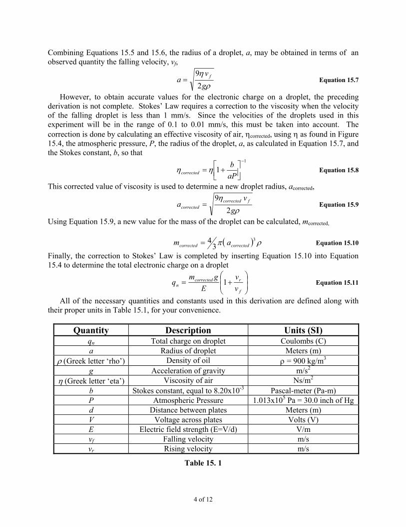
Combining Equations 15.5 and 15.6, the radius of a droplet, a, may be obtained in terms of an observed quantity the falling velocity, vf,

ρηgv

a f

29

= Equation 15.7

However, to obtain accurate values for the electronic charge on a droplet, the preceding derivation is not complete. Stokes’ Law requires a correction to the viscosity when the velocity of the falling droplet is less than 1 mm/s. Since the velocities of the droplets used in this experiment will be in the range of 0.1 to 0.01 mm/s, this must be taken into account. The correction is done by calculating an effective viscosity of air, ηcorrected, using η as found in Figure 15.4, the atmospheric pressure, P, the radius of the droplet, a, as calculated in Equation 15.7, and the Stokes constant, b, so that

1

1−

+=

aPb

corrected ηη Equation 15.8

This corrected value of viscosity is used to determine a new droplet radius, acorrected,

ρη

gv

a fcorrectedcorrected 2

9= Equation 15.9

Using Equation 15.9, a new value for the mass of the droplet can be calculated, mcorrected,

( ) ρπ 3

34

correctedcorrected am = Equation 15.10

Finally, the correction to Stokes’ Law is completed by inserting Equation 15.10 into Equation 15.4 to determine the total electronic charge on a droplet

+=

f

rcorrectedn v

vE

gmq 1 Equation 15.11

All of the necessary quantities and constants used in this derivation are defined along with their proper units in Table 15.1, for your convenience.

Quantity Description Units (SI) qn Total charge on droplet Coulombs (C) a Radius of droplet Meters (m)

ρ (Greek letter ‘rho’) Density of oil ρ = 900 kg/m3 g Acceleration of gravity m/s2

η (Greek letter ‘eta’) Viscosity of air Ns/m2 b Stokes constant, equal to 8.20x10-3 Pascal-meter (Pa-m) P Atmospheric Pressure 1.013x105 Pa = 30.0 inch of Hg d Distance between plates Meters (m) V Voltage across plates Volts (V) E Electric field strength (E=V/d) V/m vf Falling velocity m/s vr Rising velocity m/s

Table 15. 1

4 of 12

3. Laboratory Work 3.1 Apparatus Description

The apparatus used in this laboratory is a complete instrument provided by a manufacturer (see Figure 15.2). It consists of two parallel brass plates approximately one-fourth inch thick and approximately two inches in diameter. This assembly is in turn enclosed in a cylindrical plastic housing containing two windows, one for illumination of the drops and one for observation. The top plate has a small hole in its center that allows for the admission of oil droplets, which are produced by spraying oil with an atomizer (like an old perfume bottle).

To charge the plates, a power supply and a reversing switch are used; the plates are shunted by a resistor to prevent them from remaining charged when the switch is open. For observing the small oil droplets a microscopic element is used with illumination provided by a halogen lamp and condensing lens. The lamp provides back lighting so that the droplets can be seen from the light that scatters off of them. To avoid convection currents inside the apparatus, a heat absorbing filter is placed in the illuminating beam’s path.

Figure 15.2

5 of 12

The velocity of an observed droplet is determined by measuring the time required for the droplet to cover a specified number of divisions of the microscope scale (0.5mm major divisions, 0.1mm minor divisions). Care must be taken to avoid drafts and vibrations near the apparatus as the droplet might wander out of the field of view of the microscope.

Under the influence of gravity, droplets will fall at various limiting speeds. If the plates are charged, some of the drops will move down more rapidly, whereas others will reverse their direction of motion since in the process of spraying some droplets become positively charged and others negatively charged. By concentrating on one droplet, which can be controlled by the field, and manipulating the sign of the electric field so that this particular droplet is retained, it is possible to make multiple measurements of the rising and falling velocities, and from this calculate the electronic charge on this particular droplet. It is desirable to make measurements of as many different droplets as possible in order to better determine the discrete nature of the electronic charge.

Figure 15.3

3.2 Procedure 1. Level the apparatus by adjusting the leveling screws so that the air bubble is at the center of

the bubble level (see Figure 15.2). 2. Take apart the Droplet Viewing Chamber (see Figure 15.3 for an exploded view) and

carefully clean the brass plates, plastic spacer, inside surface of the chamber and other small components with soap and water. It is important to start with a clean apparatus – make sure you clean out the small hole in the top brass plate as the oil droplets must be able to flow through this orifice. Dry all the elements and reassemble. This would be a good time to measure the plate spacing, d, and record it in Section 4.2.

6 of 12

3. Make sure that the power supply is attached to the apparatus’ voltage connectors properly

(positive to positive) as shown in Figure 15.2. Connect the 12 V DC transformer to the lamp power jack in the halogen lamp housing and plug it into a wall socket.

4. Insert the Focusing Wire into the hole in the upper capacitor and then bring the reticle into

focus by turning the reticle’s focussing ring. Note, you may want to adjust the droplet focussing ring (See Figure 15.2) to ensure that both the screen and the Focusing Wire are in focus.

5. Set the voltage on the power supply to 400V, record this in Section 4.2. Note: power output

might change during the experiment, adjust accordingly. 6. Connect the multi-meter to the thermistor connectors and measure the resistance of the

thermistor. Refer to the Thermistor Resistance Table located on the platform (or Table 15.2) to find the temperature of the lower brass plate. The measured temperature will correspond to the temperature within the droplet chamber. Record the resistance and the corresponding temperature in Section 4.2.

7. Introduce oil into the chamber. Squeeze the bulb of the oil atomizer outside of the chamber

(onto paper tissue) until oil is emitted in a fine spray. Spray one small burst of oil into the chamber through the hole in the lid. Move the ionization source lever to the Spray Droplet Position to allow air to escape from the chamber.

8. Look through the viewing microscope to see if there is a shower of droplets. If there is no oil

shower then try adjusting the angle at which the lamp light enters the chamber and the droplet focussing ring (See Figure 15.2). You may also want to lift the plastic lid once to create a small disturbance of air which can help force droplets into the viewing chamber.

9. If there are no droplets in view repeat step 8. Make sure not to spray too much oil or it will

clog the entrance in the droplet hole cover. If you spray too much oil into the chamber, you will have to clean out the Droplet Viewing chamber again!

10. When you see a shower of drops through the viewing scope, move the ionization source lever

to the OFF position. 11. From the shower of drops in view, select a droplet that falls slowly and changes direction

when the Plate Charging Switch is changed from - or +. For an applied voltage of 400V, a slowly moving droplet is one with a rising time of ~ 5sec per 0.5mm and a falling time of ~ 40sec per 0.5mm. Note: If too many droplets are in view, you can clear out many of them by connecting the power to the parallel plates for several seconds which will sweep many of the droplets out of your range of view.

12. When you find an appropriately sized and charged oil droplet, fine tune the focus of the

viewing scope. Note: Make sure that the gravitational field is perpendicular to the apparatus so droplets will not drift out of focus (i.e. step 1 is really important!)

7 of 12

13. Measure the rising (plates charged) and falling (plates not charged) velocities of the selected

droplet three to four times. Maneuver the droplet as needed using the plate voltage switch. Note: The greatest accuracy of measurements is achieved if you time the interval between when the bright point of light passes behind the first major reticle line and the instant the bright point of light passes behind the second major reticle line (these lines are 0.5mm apart). The whole range of view as marked on the reticle is 3mm of separation.

14. Repeat steps 11-13 for at least two other droplets. 15. Repeat step 6 and average your temperature readings. Use this average temperature to

determine the viscosity of air, η, at the temperature of the droplet viewing chamber using Figure 15.4.

8 of 12

Name: Partners’ Names: Laboratory Section: Laboratory Section Date: Grade: Last Revised on March 30, 2003

EXPERIMENT 15

The Millikan Oil Drop Experiment 4. Post-Laboratory Work [18 pts]

4.1 Measurement Data [6pts] Record your measured times and distances for each of the droplets that you measured.

Be careful not to mix the data between the droplets.

Droplet #1 Trial #1 Trial #2 Trial #3 Trial #4 Rise Time

Rise Distance Average Rise Velocity (m/s)

Rise Velocity Fall Time

Fall Distance Average Fall Velocity (m/s)

Fall Velocity

Droplet #2 Trial #1 Trial #2 Trial #3 Trial #4 Rise Time

Rise Distance Average Rise Velocity (m/s)

Rise Velocity Fall Time

Fall Distance Average Fall Velocity (m/s)

Fall Velocity

Droplet #3 Trial #1 Trial #2 Trial #3 Trial #4 Rise Time

Rise Distance Average Rise Velocity (m/s)

Rise Velocity Fall Time

Fall Distance Average Fall Velocity (m/s)

Fall Velocity

9 of 12

4.2 Calculations [12pts]

1. Record the temperature, distance between the plates as well as the voltage across the plates below.

Temperature Initial Resistance: ____________ Initial Temperature: _______________ Final Resistance: _____________ Final Temperature: ________________ Average Temperature: _____________ Distance between the plates d: ____________

Voltage across the plates V:____________

E: ____________ 2. Calculate the uncorrected radius, a, for each of the individual droplets that you have measured using Equation 15.7. Show a sample calculation below. (2pts)

Droplet fv (m/s) η (Ns/m2) g (m/s2) ρ (kg/m3) a (m)

#1 #2 #3

3. Calculate the corrected viscosity, ηcorrected, of each of the individual droplets that you measured using Equation 15.8. Show a sample calculation below. (2pts)

Droplet η (Ns/m2) P (Pa) a (m) ηcorrected (Ns/m2) #1 #2 #3

10 of 12

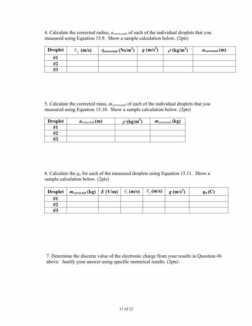
4. Calculate the corrected radius, acorrected, of each of the individual droplets that you measured using Equation 15.9. Show a sample calculation below. (2pts)

Droplet fv (m/s) ηcorrected (Ns/m2) g (m/s2) ρ (kg/m3) acorrected (m)

#1 #2 #3

5. Calculate the corrected mass, mcorrected, of each of the individual droplets that you measured using Equation 15.10. Show a sample calculation below. (2pts)

Droplet acorrected (m) ρ (kg/m3) mcorrected (kg)

#1 #2 #3

6. Calculate the qn for each of the measured droplets using Equation 15.11. Show a sample calculation below. (2pts) Droplet mcorrected (kg) E (V/m) rv (m/s) fv (m/s) g (m/s2) qn (C)

#1 #2 #3

7. Determine the discrete value of the electronic charge from your results in Question #6 above. Justify your answer using specific numerical results. (2pts)

11 of 12

Table 15.2 –Thermistor Resistance vs. Temperature

Celsius R (106 Ω) Celsius R (106 Ω) Celsius R (106 Ω) 10 3.239 20 2.300 30 1.774 11 3.118 21 2.233 31 1.736 12 3.004 22 2.169 32 1.700 13 2.897 23 2.110 33 1.666 14 2.795 24 2.053 34 1.634 15 2.700 25 2.000 35 1.603 16 2.610 26 1.950 36 1.574 17 2.526 27 1.902 37 1.547 18 2.446 28 1.857 38 1.521 19 2.371 29 1.815 39 1.496

e

Figure 15.4 – Viscosity (η) of Air vs. Temperatur

15 16 17 18 19 20 21 22 23 24 25 26 27 28 29 30 31 321.8001.8051.8101.8151.8201.8251.8301.8351.8401.8451.8501.8551.8601.8651.8701.8751.880

Visc

osity

( x1

0 -5 N

-s/m

2 )

Temperature ( oC)

12 of 12