Laslett self-field tune spread calculation with momentum dependence (Application to the PSB at 160 MeV) M. Martini

Laslett self-field tune spread calculation with momentum dependence

(Application to the PSB at 160 MeV)

M. Martini

2

Contents

06/07/2012 M. Martini

• Two-dimensional binomial distributions

• Projected binomial distributions

• Laslett space charge self-field tune shift

• Laslett space charge tune spread with momentum

• Application to the PSB

3

Two-dimensional binomial distributions

06/07/2012 M. Martini

11for0

11for1

),,,,(

2

2

2

2

2

2

2

21

2

2

2

2

2

yx

yx

m

yxyxyx

BD

a

y

a

x

a

y

a

x

a

y

a

x

aa

m

yxaam

x,yuuuma uyxyx 22,, and22with

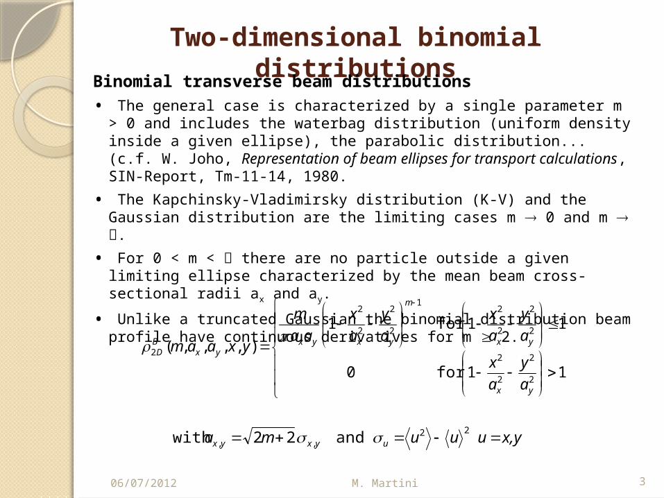
Binomial transverse beam distributions

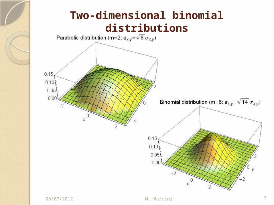
• The general case is characterized by a single parameter m > 0 and includes the waterbag distribution (uniform density inside a given ellipse), the parabolic distribution... (c.f. W. Joho, Representation of beam ellipses for transport calculations, SIN-Report, Tm-11-14, 1980.

• The Kapchinsky-Vladimirsky distribution (K-V) and the Gaussian distribution are the limiting cases m 0 and m .

• For 0 < m < there are no particle outside a given limiting ellipse characterized by the mean beam cross-sectional radii ax and ay.

• Unlike a truncated Gaussian the binomial distribution beam profile have continuous derivatives for m 2.

4


06/07/2012 M. Martini

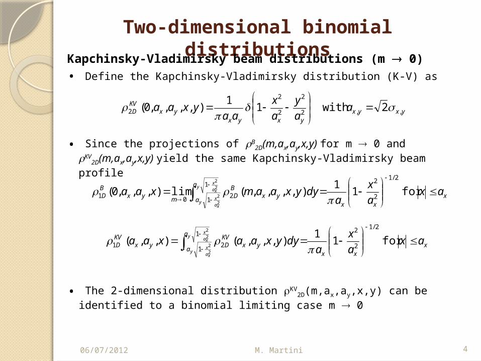
Kapchinsky-Vladimirsky beam distributions (m 0)

• Define the Kapchinsky-Vladimirsky distribution (K-V) as

• Since the projections of B2D(m,ax,ay,x,y) for m 0 and KV

2D(m,ax,ay,x,y) yield the same Kapchinsky-Vladimirsky beam profile

• The 2-dimensional distribution KV2D(m,ax,ay,x,y) can be identified to a binomial limiting

case m 0

xxx

a

ayx

BD

myx

BD ax

a

x

adyyxaamxaa xa

xy

xa

xy

for11

),,,,(lim),,,0(2/1

2

21

12

01

2

2

2

2

xxx

a

ayx

KVDyx

KVD ax

a

x

adyyxaaxaa xa

xy

xa

xy

for11

),,,(),,(2/1

2

21

121

2

2

2

2

yxyxyxyx

yxKVD a

a

y

a

x

aayxaa ,,2

2

2

2

2 2with11

),,,,0(

5


06/07/2012 M. Martini

6


06/07/2012 M. Martini

7


06/07/2012 M. Martini

8


06/07/2012 M. Martini

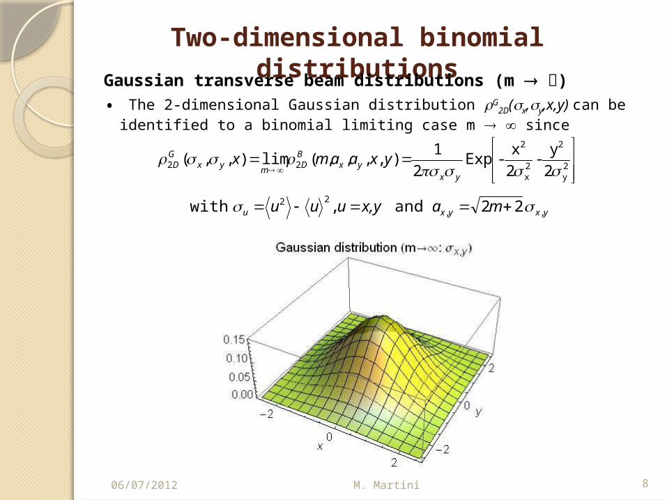
Gaussian transverse beam distributions (m )

• The 2-dimensional Gaussian distribution G2D(x,y,x,y) can be identified to a binomial

limiting case m since

2y

2

2x

2

22 2

y-

2

x-Exp

2

1),,,,(lim),,(

yxyx

BD

myx

GD yxaamx

yxyxu max,yuuu ,,

22 22and,with

9

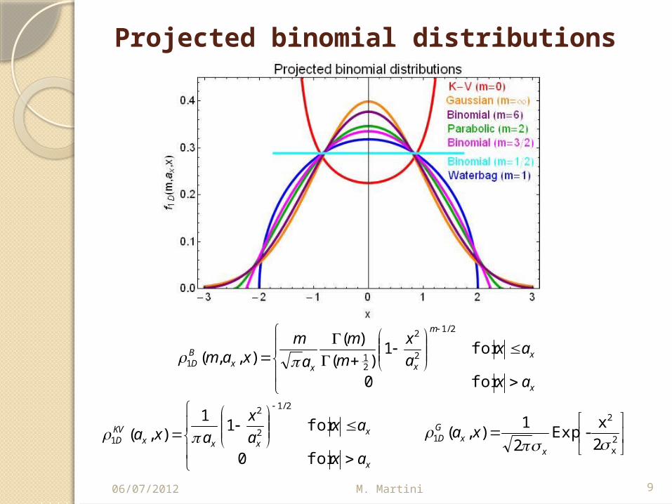
Projected binomial distributions

06/07/2012 M. Martini

x

x

m

xxxBD

ax

axa

x

m

m

a

mxam

for0

for1)(

)(),,(

2/1

2

2

21

1

x

xxxx

KVD

ax

axa

x

axa

for0

for11

),(

2/1

2

2

1

2x

2

1 2

x-Exp

2

1),(

x

xGD xa

10

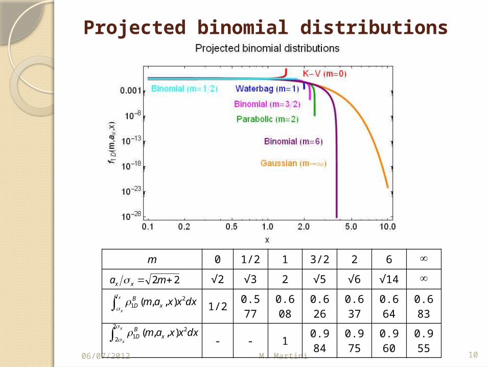
Projected binomial distributions

06/07/2012 M. Martini

m 0 1/2 1 3/2 2 6

√2 √3 2 √5 √6 √14

1/2 0.577 0.608 0.626 0.637 0.664 0.683

- - 1 0.984 0.975 0.960 0.955

x

x

dxxxam xBD

2

1 ),,(

22 ma xx

x

x

dxxxam xBD

2

2

21 ),,(

11

Laslett space charge self-field tune shift

06/07/2012 M. Martini

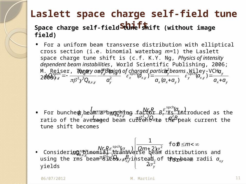
Space charge self-field tune shift (without image field)

• For a uniform beam transverse distribution with elliptical cross section (i.e. binomial waterbag m=1) the Laslett space charge tune shift is (c.f. K.Y. Ng, Physics of intensity dependent beam instabilities, World Scientific Publishing, 2006; M. Reiser, Theory and design of charged particle beams,Wiley-VCH, 2008).

• For bunched beam a bunching factor Bf is introduced as the ratio of the averaged beam current to the peak current the tune shift becomes

• Considering binomial transverse beam distributions and using the rms beam sizes x,y instead of the beam radii ax,y yields

f2

,spch,

,,0320spch

,,0peak

average )(

Ba

a

Q

RNrQ

I

IB

y

yxyx

yxyxf

yx

yyxy

yxx

yyxx

y

yxyx

yxyx aa

aa

aaa

aa

a

a

Q

RNrQ

)(

)()(

)(,

spch2

,spch

2

,spch,

,,0320spch

,,0

m

mm

BQ

RNrQ

y

y

yx

yxyxyx

for 2

1

0for)22(

1)(

2

2

f,,032

,spch,0spch

,,0

12


06/07/2012 M. Martini

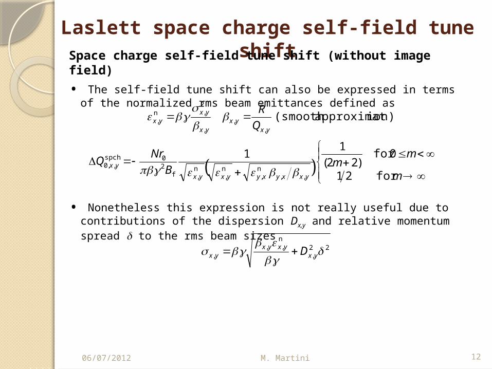
Space charge self-field tune shift (without image field)

• The self-field tune shift can also be expressed in terms of the normalized rms beam emittances defined as

• Nonetheless this expression is not really useful due to contributions of the dispersion Dx,y and relative momentum spread to the rms beam sizes

ion)approximat(smooth,

,,

2,n

,yx

yxyx

yxyx Q

R

m

mm

B

NrQ

yxxyxyyxyx

yx

for 21

0for)22(

11

,,n,

n,

n,f

20spch

,,0

22,

n,,

,

yxyxyx

yx D

13


06/07/2012 M. Martini

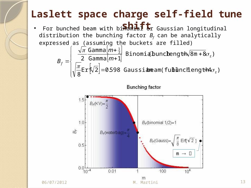
)4lengthbunch (fullbeamGaussian598.02Erf

8

)88mlength(bunch Binomial1Gamma

Gamma

2

z

z21

m

m

B f

• For bunched beam with binomial or Gaussian longitudinal distribution the bunching factor Bf can be analytically expressed as (assuming the buckets are filled)

m

14

Laslett space charge tune spread with momentum

06/07/2012 M. Martini

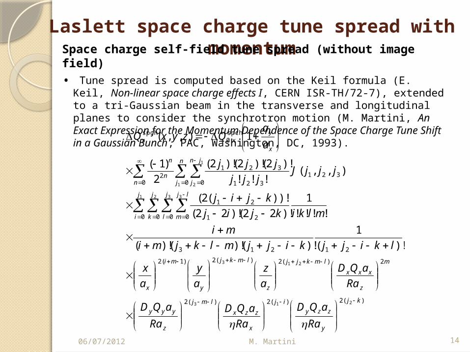
Space charge self-field tune spread (without image field)

• Tune spread is computed based on the Keil formula (E. Keil, Non-linear space charge effects I, CERN ISR-TH/72-7), extended to a tri-Gaussian beam in the transverse and longitudinal planes to consider the synchrotron motion (M. Martini, An Exact Expression for the Momentum Dependence of the Space Charge Tune Shift in a Gaussian Bunch, PAC, Washington, DC, 1993).

)(2)(2)(2

2)(2)(2)1(2

21213

0 0 0 0 21

21

0 0321

321

321

02

spch,0

spch

213

213

1 2 3 3

1

1

2

)!(

1

)!()!()!(

!!!!

1

)!22()!22(

))!(2(

),,(!!!

)!2()!2()!2(

2

)1(

1),,(

kj

y

zzy

ij

x

zzx

lmj

z

yyy

m

z

xxx

lmkjj

z

lmkj

y

mi

x

j

i

j

k

j

l

lj

m

n

j

jn

jnn

n

x

yxx

Ra

aQD

Ra

aQD

Ra

aQD

Ra

aQD

a

z

a

y

a

x

lkijjkijjmlkjmi

mi

mlkikjij

kjij

jjjJjjj

jjj

a

aQzyxQ

15

Laslett space charge tune spread with momentum

06/07/2012 M. Martini

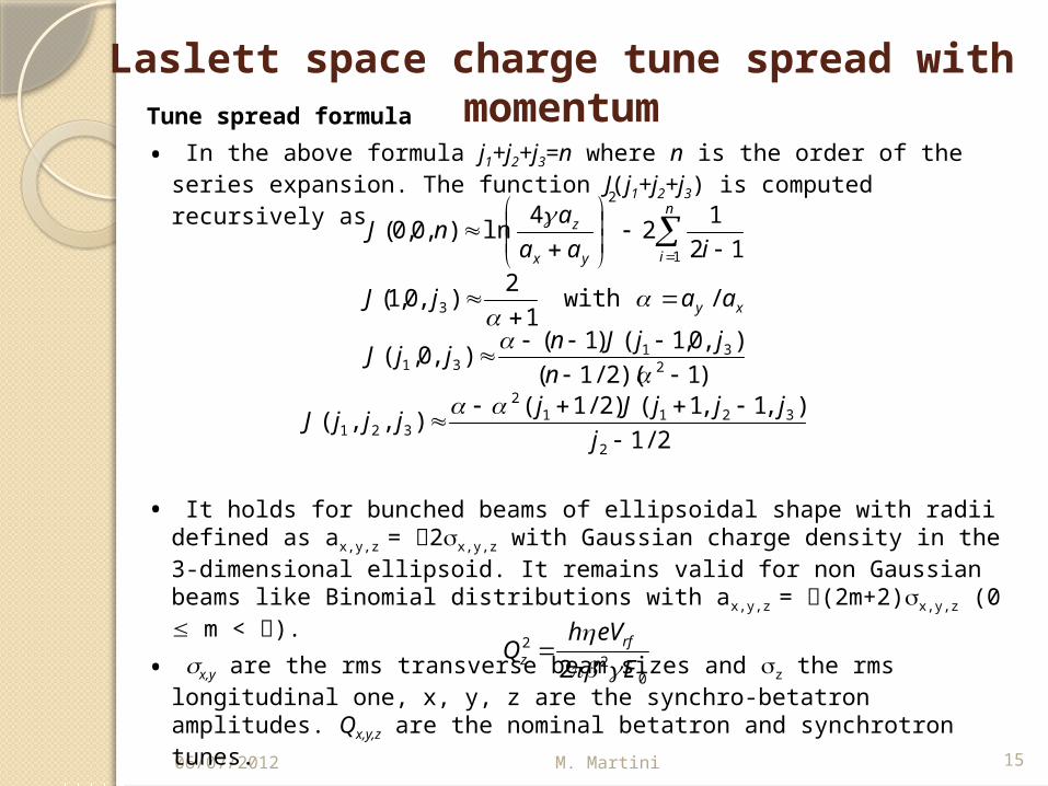
Tune spread formula

• In the above formula j1+j2+j3=n where n is the order of the series expansion. The function J(j1+j2+j3) is computed recursively as

• It holds for bunched beams of ellipsoidal shape with radii defined as ax,y,z = 2x,y,z with Gaussian charge density in the 3-dimensional ellipsoid. It remains valid for non Gaussian beams like Binomial distributions with ax,y,z = (2m+2)x,y,z (0 m < ).

• x,y are the rms transverse beam sizes and z the rms longitudinal one, x, y, z are the synchro-betatron amplitudes. Qx,y,z are the nominal betatron and synchrotron tunes.

• R is the machine radius, the other parameters Dx,y, , e, h, E0... are the usual ones.

2/1

),1,1()2/1(),,(

)1)(2/1(

),0,1()1(),0,(

/with1

2),0,1(

12

12

4ln),0,0(

2

32112

321

231

31

3

1

2

j

jjjJjjjjJ

n

jjJnjjJ

aajJ

iaa

anJ

xy

n

iyx

z

02

2

2 E

eVhQ rf

z

16

Application to the PSB

06/07/2012 M. Martini

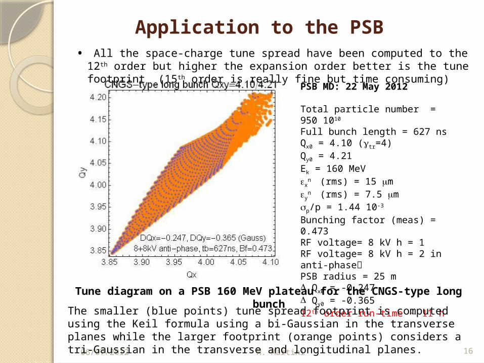
Tune diagram on a PSB 160 MeV plateau for the CNGS-type long bunch

PSB MD: 22 May 2012

Total particle number = 950 1010

Full bunch length = 627 nsQx0 = 4.10 (tr=4)Qy0 = 4.21Ek = 160 MeVx

n (rms) = 15 my

n (rms) = 7.5 mp/p = 1.44 10-3

Bunching factor (meas) = 0.473RF voltage= 8 kV h = 1RF voltage= 8 kV h = 2 in anti-phasePSB radius = 25 mD Qx0 = -0.247D Qy0 = -0.36512th order run-time 11 h

The smaller (blue points) tune spread footprint is computed using the Keil formula using a bi-Gaussian in the transverse planes while the larger footprint (orange points) considers a tri-Gaussian in the transverse and longitudinal planes.

• All the space-charge tune spread have been computed to the 12 th order but higher the expansion order better is the tune footprint (15th order is really fine but time consuming)

1706/07/2012 M. Martini

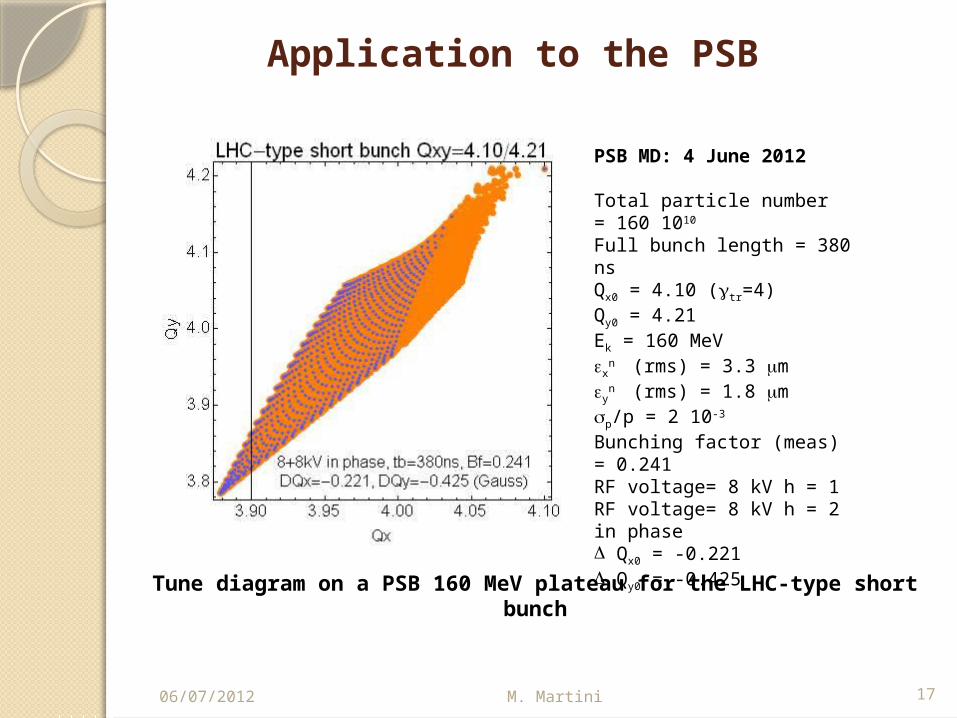
PSB MD: 4 June 2012



n (rms) = 3.3 my

n (rms) = 1.8 mp/p = 2 10-3

Bunching factor (meas) = 0.241RF voltage= 8 kV h = 1RF voltage= 8 kV h = 2 in phaseD Qx0 = -0.221D Qy0 = -0.425

Tune diagram on a PSB 160 MeV plateau for the LHC-type short bunch


1806/07/2012 M. Martini

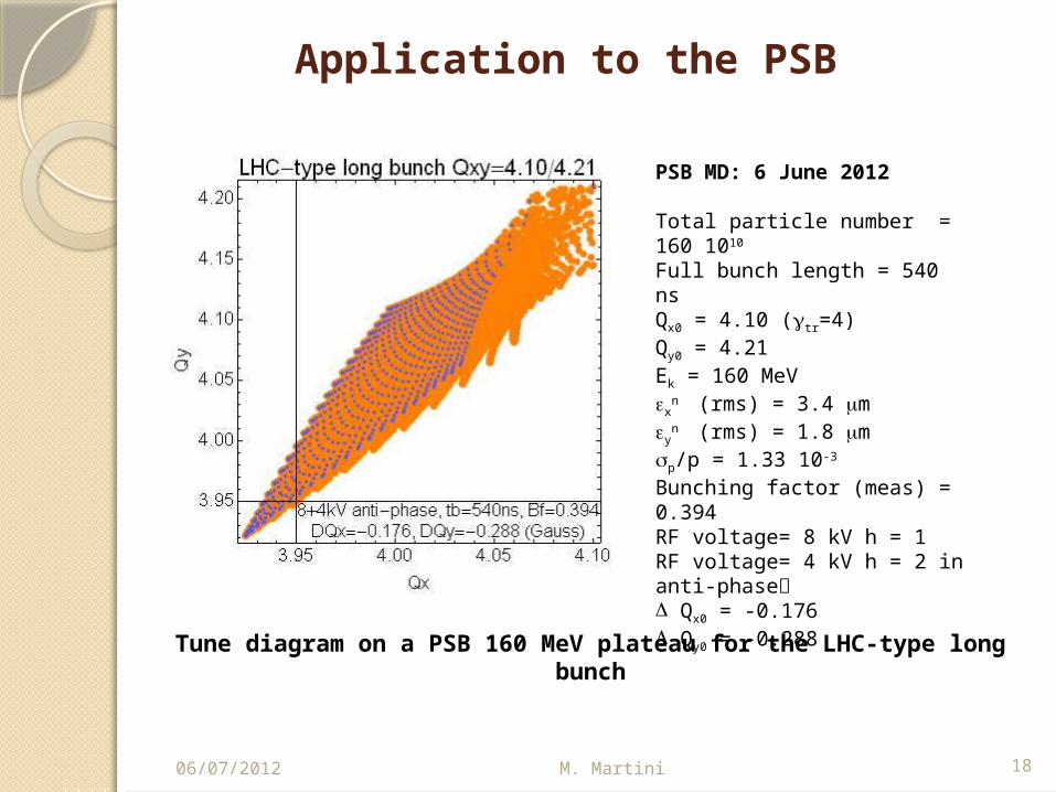
PSB MD: 6 June 2012



n (rms) = 3.4 my

n (rms) = 1.8 mp/p = 1.33 10-3

Bunching factor (meas) = 0.394RF voltage= 8 kV h = 1RF voltage= 4 kV h = 2 in anti-phaseD Qx0 = -0.176D Qy0 = -0.288

Tune diagram on a PSB 160 MeV plateau for the LHC-type long bunch


Documents

Laslett self-field tune spread calculation with momentum dependence (Application to the PSB at 160 MeV) M. Martini