Large Scale Structure in the SDSS DR1 Galaxy Surveylss.fnal.gov/archive/2003/pub/fermilab-pub-03-253-a.pdf · A. Doroshkevich et al.: Large Scale Structure in the SDSS DR1 Galaxy

arX

iv:a

stro

-ph/

0307

233v

1 1

1 Ju

l 200

3Astronomy & Astrophysics manuscript no. sdss February 2, 2008(DOI: will be inserted by hand later)

Large Scale Structure in the SDSS DR1 Galaxy Survey

A. Doroshkevich1,2, D.L. Tucker3, S. Allam3,4, and M.J. Way1,5

1 Theoretical Astrophysics Center, Juliane Maries Vej 30, DK-2100 Copenhagen Ø, Denmark2 Keldysh Institute of Applied Mathematics, Russian Academy of Sciences, 125047 Moscow, Russia3 Fermi National Accelerator Laboratory, MS 127, P.O. Box 500, Batavia, IL 60510 USA4 National Research Institute for Astronomy & Geophysics, Helwan Observatory, Cairo, Egypt5 NASA Ames Research Center, Space Sciences Division, MS 245-6, Moffett Field, CA 94035, USA

Received ..., 2003/Accepted ..., 2003

Abstract. The Large Scale Structure in the galaxy distribution is investigated using The First Data Release ofthe Sloan Digital Sky Survey. Using the Minimal Spanning Tree technique we have extracted sets of filaments,of wall–like structures, of galaxy groups, and of rich clusters from this unique sample. The physical propertiesof these structures were then measured and compared with the statistical expectations based on the Zel’dovich’theory.The measured characteristics of galaxy walls were found to be consistent with those for a spatially flat ΛCDMcosmological model with Ωm ≈ 0.3 and ΩΛ ≈ 0.7, and for Gaussian initial perturbations with a Harrison –Zel’dovich power spectrum. Furthermore, we found that the mass functions of groups and of unrelaxed structureelements generally fit well with the expectations from Zel’dovich’ theory. We also note that both groups and richclusters tend to prefer the environments of walls, which tend to be of higher density, rather than the environmentsof filaments, which tend to be of lower density.

Key words. cosmology: large-scale structure of the Universe: general — surveys

1. Introduction

With the advent of the Durham/UKST Galaxy RedshiftSurvey (DURS, Ratcliffe et al. 1996) and the LasCampanas Redshift Survey (LCRS, Shectman et al.1996), the galaxy distribution on scales up to ∼300h−1 Mpc could be studied. Now these investigations canbe extended using the public data sets from The FirstData Release of the Sloan Digital Sky Survey (SDSS DR1,Stoughton et al. 2002; Abazajian et al. 2003), which con-tains redshifts for ≈ 100 000 galaxies in four slices for dis-tances D ≤ 600h−1Mpc.

The analysis of the spatial galaxy distribution in theDURS and the LCRS has revealed that the Large ScaleStructure (LSS) is composed of walls and filaments, thatgalaxies are divided roughly equally into each of thesetwo populations (with few or no truly isolated galax-ies), and that richer walls are linked to the joint ran-dom network of the cosmic web by systems of filaments(Doroshkevich et al. 2000, 2001). Furthermore, these find-ings are consistent with results obtained for simulations ofdark matter (DM) distributions (see e.g. Cole et al. 1998;Jenkins et al. 1998) and for mock galaxy catalogues basedupon DM simulations (Cole et al. 1998).

The quantitative statistical description of the LSS isin itself an important problem. Beyond that, though, the

analysis of rich catalogues can also provide estimates forcertain cosmological parameters and for the characteris-tics of the initial power spectrum of perturbations. To doso, some theoretical models of structure formation can beused.

The close connection between the LSS and Zel’dovich’pancakes has been discussed by Thompson & Gregory(1978) and by Oort (1983). Now this connection is ver-ified by the comparison of the statistical characteris-tics of observed and simulated walls with theoretical ex-pectations (Demianski & Doroshkevich 1999, 2002, here-after DD99 and DD02) based on the Zel’dovich theoryof nonlinear gravitational instability (Zel’Dovich 1970;Shandarin & Zeldovich 1989). This approach connects thecharacteristics of the LSS with the main parameters ofthe underlying cosmological scenario and the initial powerspectrum, and it permits the estimation of some of theseparameters using the measured properties of walls. It wasexamined with the simulated DM distribution (DD99;Demianski et al. 2000), and was found that, for sufficientlyrepresentative samples of walls, a precision of better than20% can be reached.

Effective methods of the statistical description of theLSS based on the Minimal Spanning Tree (MST) tech-nique were developed by Demianski et al. (2000) and

http://arXiv.org/abs/astro-ph/0307233v1

2 A. Doroshkevich et al.: Large Scale Structure in the SDSS DR1 Galaxy Survey

Fig. 1. Four regions of the DR1 sample on the sky.

Doroshkevich et al. (2000, 2001), who applied them toDM simulations and to the DURS and the LCRS.These methods introduced in Barrow et al. (1985) andvan de Weygaert (1991) generalize the popular ”friends-of-friends” approach. In this paper we apply the sameapproach to the SDSS DR1, a sample from which wecan obtain more representative and more precise mea-sures of the properties of the LSS and the initial powerspectrum of perturbations. Alternative methods basedon Minkowski functionals are proposed by, for example,Schmalzing et al. (1999), or Sheth et al. (2002)

With the MST technique, we can quantitatively de-scribe the sample under investigation and divide the sam-ple into physically motivated subsamples of clusters withvarious threshold overdensities bounding them. Then wecan extract the LSS elements and characterize their mor-phology. In particular, this technique allows us to discrimi-nate between filamentary and wall–like structure elementslocated presumably within low and high density regionsand to estimate their parameters for the different thresh-old overdensities. The same technique allows us to extractsets of high density groups of galaxies and to measuresome of their properties.

The analysis of wall-like condensations is most in-formative. Comparison of the observed characteristics ofwalls with theoretical expectations (DD99; DD02) demon-strates that the observed galaxy distribution is consistentwith Gaussianity initial perturbations and that the wallsare the recently formed, partly relaxed Zel’dovich’ pan-cakes. The mean basic characteristics of the walls areconsistent with those theoretically expected for the ini-tial power spectrum measured by the CMB observationssummarized, for example, in Spergel et al. (2003).

In this paper we also analyse the mass functions ofstructure elements selected for a variety of boundary

Fig. 2. The radial galaxies distributions in the four sam-ples of the SDSS DR1. The selection function (1) is plottedby solid lines.

threshold overdensities. We show that these functions arequite similar to the expectations of Zel’dovich’ theory,which generalizes the Press – Shechter formalism for anystructure elements. In addition, the theory indicates thatthe interaction of large and small scale perturbations canbe important for the formation of the observed LSS massfunctions. Our analysis demonstrates that this interactionis actually seen in the influence of environment on thecharacteristics of groups of galaxies. This problem was alsodiscussed in Einasto et al. (2003a,b).

This paper is organized as follows: In Secs. 2 we de-scribe the sample of galaxies which we extracted from theSDSS DR1 and the method we have employed to correctfor radial selection effects. In Sec. 3 we establish the gen-eral characteristics of the LSS. More detailed descriptionsof the filamentary network and walls can be found in Secs.4 and 5, respectively. In Secs. 6 and 7 we discuss the prob-able selected clusters of galaxies and the mass function ofstructure elements. We conclude with Sec. 8 where a sum-mary and a short discussion of main results are presented.

2. The First Data Release of the Sloan Digital

Sky Survey

We use as our observational sample the SDSS DR1(Abazajian et al. 2003), which is the first public releaseof data from the SDSS (Fukugita et al. 1996; Gunn et al.1998; York et al. 2000). The imaging data for the SDSSDR1 encompasses 2099 sq deg of sky. The DR1 also con-tains 186,240 follow up spectra, which are available over1360 sq deg of the imaging data area. Galaxies are sit-uated within two north fields, N1 & N2, and two southfields, S1 & S2. These regions are plotted in Fig. 1 .

A. Doroshkevich et al.: Large Scale Structure in the SDSS DR1 Galaxy Survey 3

Fig. 3. The wedge diagram of galaxy distributions in thesamples S1 is real (top panel) and modified (bottom panel)radial coordinates.

We obtained our SDSS DR1 sample via the SDSS DR1Spectro query server 1. This is a web interface to the SDSSCatalog Archive Server. We selected all objects identifiedas galaxies with a ‘redshift confidence minimal level’ of95% and no maximal level. No other constraints in theselection were made at this level.

Our method for detecting LSS depends on havinglargely contiguous regions. Hence we have removed someregions and artifacts from the DR1 sample. The follow-ing are the RA and DEC areas we masked out from theoriginal DR1 query before our analysis:

• 174h<RA<179h, -4.0

<DEC<-1.22

• 159h<RA<163h, 1.1

<DEC<4.0

• 10h<RA<50h, 10

<DEC<20

• 300h<RA<355h, -12

<DEC<-4

• 250h<RA<270h, 52

<DEC<67

2.1. Correction for radial selection effects

In Figure 2 we plot the radial distributions of galaxiesin all four samples. In Figure 3 we plot the wedge di-agramm of observed galaxy distribution for the sampleS1. As is clearly seen from these Figures, at distancesD ≥ 400h−1Mpc this fraction of observed galaxies isstrongly suppressed because of the radial selection ef-fect. Note that this suppression is quite successfully fitby curves describing a selection function of the form

fgal(D) ∝ D2 exp[−(D/Rsel)3/2], Rsel ≈ 190h−1Mpc ,(1)

1 http://www.sdss.org/dr1

Fig. 4. The normalized mean galaxy density in the fourmodified samples of SDSS DR1.

where D is a galaxy’s radial distance and Rsel is the selec-tion scale (Baugh & Efstathiou 1993). These fits are alsoplotted in Fig. 2.

In some applications, like when we want to correct ameasure of the observed density to a measure of the truedensity, we would like to use equation (1) to correct for theradial selection effects after the fact. An example of sucha case is calculating a group’s or cluster’s true richnessbased upon the observed number of galaxies it contains(Sec. 6 & 7). modified

In other applications, however, like in searching forgroups or clusters in a magnitude-limited sample, we wantto make a preemptive correction for the radial selection ef-fects. For example, in a standard friends-of-friends perco-lation algorithm (e.g. Huchra & Geller 1982), this is doneby adjusting the linking length as a function of radial dis-tance. Here, instead, we employ the rather novel approachof adjusting the radial distances themselves as introducedand discussed in Doroshkevich et al. (2001). Hence, in-stead of the measured radial distance, we use a modifiedradial distance, Dmd, where

D3

md = 2R3

sel(1 − [1 + (D/Rsel)3/2] exp[−(D/Rsel)

3/2]) .(2)

The radial variations of the normalized number density ofgalaxies for all samples from Figure 2 are plotted in Figure4. As is seen from this figure, the modified radial distancesfor the galaxies suppresses the very large-scale trends. Onthe other hand the relative position of galaxies remainunchanged and the smaller scale random variations in thedensity are emphasized. The wedge diagramm of modifiedgalaxy distribution for the sample S1 is also plotted inFig. 3.

This correction does not change distances at D ≤ Rsel

and is more important for the more distant regions of oursamples (D ≥ 350h−1Mpc), which contain only ∼20% of

http://www.sdss.org/dr1


all galaxies. Thus, in the following analyses, we apply thiscorrection only to the separation of the high and low den-sity regions in the deeper samples. Of course, it cannotrestore the lost information about the galaxy distributionin these regions, but it does help compensate for the strongdrop in the observed galaxy density at these distances. Italso allows one to apply the standard methods of investi-gation for the full catalogues with a depth of 600h−1Mpc.

3. General characteristics of observed large scale

structure

To characterize the general properties of the large scalespatial galaxy distribution we use the Minimal SpanningTree (MST) technique applied to both directly observedsamples of galaxies and to samples corrected for the selec-tion effect.

In our analysis here, we consider the four fields, plottedin Fig. 1, at the distance D ≤ 420h−1Mpc with

Ngal = 79 183, 〈ngal〉 ≈ 10−2Mpc−3 , (3)

where Ngal and 〈ngal〉 are the total number of galaxiesand the mean density of the samples. This sample contains≈85% of all galaxies with moderate impact from selectioneffects. The numbers of galaxies in the separate fields are

– N1, the northern sample (35 520 galaxies)– N2, the northern sample (21 983 galaxies)– S1, the southern sample (11 225 galaxies)– S2, the southern sample (10 455 galaxies)

3.1. The MST technique

The MST technique was first discussed by Barrow et al.(1985) and by van de Weygaert (1991). The MST is a con-struct from graph theory, originally introduced by Kruskal(1956) and Prim (1957), which has been widely applied intelecommunications and similar fields. It is a unique net-

work associated with a given point sample and connects allpoints of the sample to a tree in a special and unique man-ner which minimizes the full length of the tree. Furtherdefinitions, examples, and applications of this approachare discussed in Barrow et al. (1985) and van de Weygaert(1991). More references to the mathematical results canalso be found in van de Weygaert (1991).

One of earliest uses of MST approach in the study oflarge-scale structure was that of Bhavsar & Ling (1988),who successfully applied it to extract filamentary struc-tures from the original CfA Redshift Survey. Its ap-plications for the quantitative description of observedand simulated catalogues of galaxies were discussed inDemianski et al. (2000); Doroshkevich et al. (2000, 2001).

One of the most important features of the MST tech-nique is generalization of the widely used “friends–of–friends” approach. It allows one to separate all clusters,LSS elements, with a given linking length. In spite ofthe very complex shape of the clusters, the linking length

defines for each two points the local overdensity bound-ing the clusters with a relation familiar from “friends–of–friends” algorithms (Huchra & Geller 1982):

δthr = 3/[4π〈ngal〉r3

lnk] . (4)

Further on it allows one to obtain characteristics of eachcluster and of the sample of clusters forming the LSS witha given overdensity. Further discrimination can be per-formed for a given threshold richness of individual ele-ments.

Here we will restrict our investigation to our resultsfor the probability distribution function of the MST edge

lengths WMST (l) and to the morphological description ofindividual clusters. The potential of the MST approach isnot, however, exhausted by these applications.

3.2. Wall-like and filamentary structure elements

With the MST technique we can demonstrate that the ma-jority of galaxies are concentrated within wall–like struc-tures and filaments which connect walls to the joint ran-dom network of the cosmic web. The internal structureof both walls and filaments is complex. Thus, wall–likestructures incorporate some fraction of filaments and bothwalls and filaments incorporate high density galaxy groupsand clouds. In particular, clusters of galaxies are usuallysituated within richer walls while groups of galaxies areembedded within filaments. In spite of this, the galaxydistribution can be described as a set of one, two andthree dimensional Poisson–like distributions. Naturally, aone dimensional distribution is more typical for filamentswhile two and three dimensional ones are typical for wallsand groups of galaxies, respectively. As was shown invan de Weygaert (1991) Buryak & Doroshkevich (1996),a Poissonian distribution of galaxies within the LSS ele-ments successfully reproduces the observed 3D correlationfunction of galaxies.

These result show that the probability distributionfunction of MST edge lengths (PDF MST), WMST (l),characterizes the geometry of the galaxy distribution. For1D and 2D Poissonian distributions, typical for filamentsand walls, WMST (l) is described by the following expo-nential and Rayleigh functions,

WMST (l) = We(l) = 〈l〉−1 exp(−l/〈l〉) , (5)

WMST (l) = WR(l) = 2l/〈l2〉 exp(−l2/〈l2〉) .

These PDFs remain valid for any 1D and 2D distributionswhen the galaxy separation is small as compared with thecurvature of the lines and surfaces. Comparison of mea-sured and expected PDFs MST allows one to demonstratethe existence of these two types of structure elementsand to make approximate estimates of their richness. Letus recall, however, that for the galaxy groups embeddedwithin filaments, 2D and 3D Poissonian distributions areobserved and, so, in this case we cannot see a purely 1Ddistribution. For walls this effect is less important because


Fig. 5. PDFs of MST edge lengths in redshift space aver-aged over four samples are plotted for the full sample (toppanel), HDRs (middle panel) and LDRs (bottom panel).Rayleigh and exponential fits are plotted by thin solid anddashed lines.

it only distorts the 2D distribution typical for such LSSelements.

In Fig. 5 (top panel) we plott the WMST (lMST )’s forthe entire sample of 79,183 galaxies situated at distancesD ≤ 420h−1Mpc where, as is seen from Fig. 2, the impactof the selection effect is still moderate. The error bars showthe scatter of measurements for the four subsamples. Foreach sample, N1, N2, S1, S2, we have

〈lMST 〉 = 2.5, 2.6, 2.3, 2.0 h−1Mpc . (6)

These variations demonstrate the differences in the sampleproperties (cosmic variance).

Notice in Fig. 5 that the WMST (lMST ) is well fit bya superposition of Rayleigh (at lMST ≤ 〈lMST 〉) and ex-ponential (at lMST ≥ 〈lMST 〉) functions. This confirmsresults discussed in Doroshkevich et al. (2000; 2001) inrespect to the high degree of galaxy concentration withinthe population of high density rich wall–like structuresand less rich filaments. However, as was noted in the samepapers, with this approach the approximate separation ofwall–like and filamentary structure elements can be per-formed only statistically. This is because the high densitypart of the PDF described by the Rayleigh function in-cludes high density clouds situated in both filaments andwalls. The exponential part of the PDF is related mainlyto the filamentary component.

3.3. High and low density regions

The methods for an approximate statistical decompositionof a sample into subsamples of wall–like structures and

filaments were proposed and tested in our previous publi-cations (Demianski et al. 2000; Doroshkevich et al. 2000,2001). The first step is to make a rough discrimination be-tween the high and low density regions (HDRs and LDRs).

Such discrimination can be easily performed for agiven overdensity contour bounding the clusters and agiven threshold richness of individual elements. FollowingDoroshkevich et al. (2001), in all four samples with D ≤420h−1Mpc, wall–like high density regions (HDRs) wereidentified with clusters found for a threshold richnessNthr = 40 and a threshold overdensity contour bound-ing the cluster equal to the mean density, δthr = 1. Thesesamples, N1, N2, S1, S2, of HDRs contain 49%, 47%, 51%and 47% of all galaxies. The samples of low density regions(LDRs), which are occupied mainly by filaments and poorgroups of galaxies, are complementary to the HDRs inthat the LDRs are simply the leftovers from the originaltotal samples after the HDRs have been removed.

In Figure 5 (middle panel) the WMST (l) plotted for theHDRs is very similar to a Rayleigh function, thus confirm-ing with this criterion the sheet-like nature of the observedgalaxy distribution within the HDRs. As before, the errorbars show the scatter of measurements for the four sub-samples. For 90% of objects we have

WHDR = (1 ± 0.18) WR, lMST ≤ 1.65〈lMST 〉 , (7)

where WR is the Rayleigh function (5). Larger differencebetween observed and expected PDFs for larger lMST in-dicates that the selected sample of HDRs includes somefraction of objects, ∼ 10%, which can be related to thefilamentary component with the exponential PDF.

For the LDRs, the WMST (l) is plotted in Fig. 5 (bot-tom panel). For small edge lengths, l ≤ 〈lMST 〉, it alsofits well to a Rayleigh function indicating that ∼ 60% ofLDR galaxies are concentrated within less massive 3D (el-liptical) and 2D (sheet-like) clouds. This result confirmsthe strong disruption of filaments to a system of high den-sity clouds. For larger edge lengths, however, the LDRWMST (l) appears to be closer to an exponential function,indicating that according to this criterion the spatial dis-tribution of the remaining ∼ 40% of LDR galaxies is simi-lar to a 1D Poissonian one which is typical for filamentarystructures.

The mean edge lengths, 〈lMST 〉, found for HDRs andLDRs in samples N1, N2, S1, S2 are

〈lMST 〉 = 1.2, 1.3, 1.2, 1.3 h−1Mpc , (8)

〈lMST 〉 = 2.8, 2.7, 2.6, 2.8 h−1Mpc . (9)

These values differ by about a factor of two from eachother, indicating that, as is seen from (4), the differencein the mean density within HDRs and LDRs elements isabout an order of magnitude. Of course, the volume aver-aged density of LDRs is still less.


Fig. 6. Mass functions of structure elements, fm(ǫ), ǫ =Ltr/Lsum for the structure elements selected within HDRs(top panel, solid and dashed lines) and within LDRs (bot-tom panel, solid and dashed lines).

3.4. Morphology of the structure elements

Within so defined HDRs and LDRs themselves we canextract with the MST technique subsamples of structureelements for various threshold overdensities. We can thensuitably characterize the morphology of each structure el-ement by comparing the sum all edge lengths within itsfull tree, Lsum, with the sum of all edge lengths withinthe tree’s trunk, Ltr, which is the longest path that canbe traced along the tree without re-tracing any steps. Theratio of these lengths

ǫ = Ltr/Lsum . (10)

suitably characterizes the morphology of the LSS ele-ments.

For filaments, we can expect that the lengths of thefull tree and of the trunk are similar to each other, ǫ ∼ 1,whereas for clouds and walls these lengths are certainlyvery different and ǫ ≤ 1. This approach takes into ac-count the internal structure of each element rather thanthe shape of the isodensity contour bounding it, and in thisrespect it is complementary to the Minkowski Functionaltechnique (e.g. Schmalzing et al. 1999; Sheth et al. 2002).

However, even this method cannot discriminate be-tween the wall–like and 3D (elliptical) clouds and thoserich filaments having many long branches for which againǫ ≤ 1. This means that both the PDF of this ratio, W (ǫ),and the corresponding mass function, fm(ǫ), are contin-uous functions and the morphology of structure elementscan be more suitably characterized by the degree of fil-amentarity and ‘wall-ness’. This also means that we canonly hope to distinguish statistical differences between the

morphologies of structure elements in HDRs and the mor-phologies of structure elements in LDRs.

The selection of clusters within HDRs and LDRswas performed for two threshold linking lengths, rlnk =2. & 2.4h−1Mpc for HDRs, and rlnk = 3.2 & 3.6h−1Mpcfor LDRs. These values are larger than the mean edgelengths and characterize the LSS elements with interme-diate richness when the measured difference between thewalls and filaments is maximal. As was noted above, forlower linking lengths this method characterizes mainly theinternal structure of the LSS elements while for large link-ing lengths filaments percolate and form the joint networkwith again ǫ ≪ 1.

The distribution functions of the ratio, W (ǫ), are foundto be close to Gaussian with 〈ǫ〉 ≈ 0.5 & 0.70 for HDRsand LDRs, respectively. The mass functions, fm(ǫ), plot-ted in Fig. 6 for the same linking lengths are shifted to theleft (for HDRs) and to the right (for LDRs) with respectto the middle point. Differences between these functionsfound for smaller and larger linking lengths illustrate theimpact of the percolation process and disruption of theLSS elements.

These results verify the objective nature of the differ-ences in the structure morphologies in HDRs and LDRs.

4. Statistical characteristics of filaments

Theoretical characteristics of the LSS elements relate tothe dominant dark matter (DM) component while the ob-served galaxy distribution relates to the luminous matterwhich represent only ∼ 3 – 5% of the mean density ofthe Universe. Spatial distribution of dark and luminousmatter is strongly biased. None the less, some observedcharacteristics of filamentary components of the LSS canbe compared with both available theoretical expectationsand characteristics obtained for simulated DM distribu-tions.

The most interesting ones are the PDF of the lineardensity of filaments measured as the mass or number ofobjects per unit length of filament, Σfil. The other is themean surface density of filaments σfil, defined as the meannumber of filaments intersecting a unit area of arbitraryorientation. Both characteristics depend upon the thresh-old linking length, rlnk, used for the filament selectionand upon the threshold richness of filaments. However,both characteristics are independent from the small scaleclustering of matter within filaments.

Comparison of these characteristics of filaments for ob-served and simulated catalogues allows one to test the cos-mological model used. However, the connection of quan-titative characteristics of filaments with the initial powerspectrum is complex and these measurements cannot yetbe used for estimates of the power spectrum.

4.1. Linear density of filaments

As was found in DD99 and DD02, for the CDM–like initialpower spectrum the PDF of the filament linear density can


Fig. 7. Distribution function, Nfil, for the linear densityof ’galaxies’ along a tree for filaments selected in LDRs ofthe mock catalogues with three linking lengths. Fits (11)are plotted by solid lines.

be written as follows:

Nfil dΣfil ≈1.5

〈Σfil〉exp(−

√

3Σfil/〈Σfil〉) dΣfil . (11)

However, poorer filaments cannot actually be selected ineither simulated or observed catalogues. Hence, even forhigh resolution simulations the measured PDF is well fit-ted by the relation

Nfil ≈ a0 erf4[a1(x − x0)] exp[−√

a2(x − x0)] (12)

where x = Σfil/〈Σfil〉, x0 ≈ 0.35, a1 ≈ 2 − 2.5 and a2 ≈30−40 (DD02) and 〈Σfil〉 ∼ 3/rlnk. Here the cutoff of thePDF at x = x0 reflects the limited resolution of simulatedmatter distribution.

These results can be compared with ones obtained forfor the DR1 and the mock catalogue (Cole et al. 1998)which allows one to estimate the impact of the selectioneffect for the measured linear density of filaments. In boththe cases, the linear density of objects was measured bythe ratio of the number of points and the length of theMST for each filaments of the sample.

For the mock catalogue the PDFs of the linear densityof filaments are plotted in Fig. 7 for three linking length(with δthr ≈ 1, 0.7 & 0.5). These PDFs are well fitted byexpression (12) for parameters x0 ≈ 0.6, a1 ≈ 2.5, a2 ≈80− 90. For all linking lengths we get 〈Σfil〉rlnk = 2.25±0.04. For the observed DR1 catalogue the same PDFs areplotted in Fig. 8 also for three linking length (with δthr ≈50, 5 & 0.55). They are well fitted by the same expression(12) for parameters x0 ≈ 0.5, a1 ≈ 2.5, a2 ≈ 70 − 80. Forthis sample we get 〈Σfil〉rlnk = 2.2 ± 01.

These results show that, in all the cases, the mea-sured PDFs are well fit by the same expression (12)

Fig. 8. Distribution function, Nfil, for the linear densityof galaxies along a tree for filaments selected in LDRs ofthe DR1 with three linking lengths. Fits (11) are plottedby solid lines.

which coincides with the theoretically expected one (11)at Σfil ≥ 〈Σfil〉. The mean linear density, 〈Σfil〉, clearlydepends upon the linking length used for filament selec-tion. The selection effect increases the product 〈Σfil〉rlnk

by ∼ 1.5 times as compared with results obtained for theDM simulations.

These results show that the observed galaxy distribu-tion nicely represents the expected and simulated ones.The results also indicate that the general properties offilaments are consistent with a CDM–like initial powerspectrum.

4.2. Typical size of the filamentary network

Due to the complex shape of the network of filamentsspanning the LDRs any definition of the typical size ofa network cell is mearly convenient. As was discussed inDoroshkevich et al. (2001), two definitions seem to be themost objective. One is the mean free path between fila-ments along a random straight line. The other is the meandistance between branch points of the tree along the trunkof selected filaments. The second definition tends to yieldcell sizes that are typically a factor of 1.5 smaller thanthose yielded by the mean-free-path definition.

Theoretical estimates of this size are uncertain be-cause it strongly depends upon the sample of selectedfilaments (DD02). This means that this characteristicstrongly depends upon the catalogue used. Moreover, fil-aments are connected to the network only for larger link-ing lengths; thus the typical measured cell size dependsalso upon the threshold linking length used. Hence, forthe LCRS the mean free path between filaments with a


Fig. 9. Distribution functions, N , for the distance betweenbranch points along a trunk for filaments selected in LDRs(thick solid and dashed lines). Fit (13) is plotted by thinsolid line.

variety of richness was estimated in Doroshkevich et al.(2001) as ∼ 13 − 30h−1Mpc. The mean distance betweenbranch points of the tree along the trunk was estimatedas ≈ 10h−1Mpc and it rapidly increases with the linkinglength used owing the progressive percolation of filamentsand formation of the joint LSS network.

Here with a richer sample of filaments we can also es-timate the PDFs of the cell sizes measured by the dis-tance between branch points of the tree along the trunk.These PDFs, N(lbr), are plotted in Fig. 9 for two linkinglengths, rlnk = 1.8 & 3.6h−1Mpc, which correspond to thethreshold overdensities δthr = 0.66 & 0.5. These PDFs areroughly fitted by expression

N(lbr) ≈ 270x4.5 exp(−9.1x), x = lbr/〈lbr〉 , (13)

The measured mean distance between branch points,

〈lbr〉 ≈ 4.7 & 11.9h−1Mpc .

are close to those obtained in Doroshkevich et al. (2001)and Doroshkevich et al. (1996) and those cited above. Forsmaller rlnk this estimate is decreased because of the dom-ination of short filaments which are not yet connected tothe network.

5. Parameters of the wall–like structure elements

The statistical characteristics of observed walls were firstmeasured using the LCRS and DURS (Doroshkevich et al.2000, 2001). The rich sample of walls extracted from theSDSS DR1, however, permits more refined estimates ofthese characteristics. As was discussed in Sec. 3.2 walls

dominate the HDRs, and thus these subsamples of galaxiescan be used to estimate the wall properties.

The expected characteristics of walls and methodsof their measurement were discussed in Demianski et al.(2000) so here we will only briefly reproduce the maindefinitions. It is important that these characteristics canbe measured independently in radial and transverse direc-tions, which reveals the strong influence of the velocitydispersion on other wall characteristics.

5.1. Main wall characteristics

Main characteristic of walls is their mean dimensionlesssurface density, 〈qw〉, measured by the number of galaxiesper Mpc2 and normalized by the mean density of galaxiesmultiplied by a coherent length of the initial velocity field(DD99; DD02)

lv ≈ 33h−1Mpc (0.2/Γ), Γ = Ωmh , (14)

where Ωm is the mean matter density of the Universe. ForGaussian initial perturbations, the expected probabilitydistribution function (PDF) of the surface density is

Nth(qw) =1√2π

1

τm√

qwexp

(

− qw

8τ2m

)

erf

(√

qw

8τ2m

)

, (15)

〈qth〉 = 8(0.5 + 1/π)τ2

m ≈ 6.55τ2

m .

This relation links the mean surface density of walls withthe dimensionless amplitude of perturbations, τm,

τm =√

〈qw〉/6.55 , (16)

which can be compared with those measured by othermethods (DD02, Sec. 8.2).

Other important characteristics of walls are the meanvelocity dispersion of galaxies within walls, 〈ww〉, themean separation between walls, 〈Dsep〉, the mean over-density, 〈δ〉, and the mean thickness of walls, 〈h〉. Themean velocity dispersion of galaxies, 〈ww〉, can be mea-sured in radial direction only whereas other wall character-istics can be measured both radially and along transversearcs. Comparison of the wall thickness and the overden-sity, 〈h〉 and 〈δ〉, measured in transverse (t) and radial (r)directions, illustrates the influence of the velocity disper-sion of galaxies on the observed wall thickness.

The velocity dispersion of galaxies within a wall ww

can be related to the radial thickness of the wall by thisrelation (Demianski et al. 2000):

hr =√

12H−1

0ww . (17)

For a relaxed, gravitationally confined wall, the mea-sured wall overdensity, surface density, and the velocitydispersion are linked by the condition of static equilib-rium. Consider a wall as a slab in static equilibrium, andthis slab has a nonhomogeneous matter distribution acrossit. We can then write the condition of static equilibriumas follows:

w2

w =πGµ2

〈ρ〉δ ΘΦ =3

8

Ωm

δ(H0lvqw)2ΘΦ , (18)


Here µ = 〈ρ〉lvqw is the mass surface density of the walland the factor ΘΦ ∼ 1 describes the nonhomogeneity ofthe matter distribution across the slab. Unfortunately, forthese estimates we can only use the velocity dispersion andoverdensity measured for radial and transverse directions.Hence, the final result cannot be averaged over the samplesof walls.

5.2. Measurement of the wall characteristics

The characteristics of the walls can be measuredwith the two parameter core–sampling approach(Doroshkevich et al. 1996) applied to the subsampleof galaxies selected within HDRs. With this method, allgalaxies of the sample are distributed within a set ofradial cores with a given angular size, θc, or within a setof cylindrical cores oriented along arcs of right ascensionwith a size dc. All galaxies are projected on the core axisand collected to a set of one-dimensional clusters with alinking length, llink. The one-dimensional clusters withrichnesses greater than some threshold richness, Nmin,are then used as the required sample of walls within asampling core.

Both the random intersection of core and walls and thenonhomogeneous galaxy distribution within walls lead tosignificant random scatter of measured wall characteris-tics. The influence of these factors cannot be eliminated,but it can be minimized for an optimal range of param-eters θc, dc, llink and Nmin. Results discussed below areaveraged over the optimal range of these parameters.

For the measurement of wall characteristics in the ra-dial direction four samples of HDRs galaxies were usedin each field of the DR1 catalogue. One of these sam-ples was selected as was discussed in Sec. 3.3, three othersamples were selected from the catalogues already cor-

rected for radial selection effects (Sec. 2.1) with the samethreshold overdensity δthr = 1 and for HDRs contain-ing ∼ 43%, 50%, and 56% of all galaxies in the field. Inall the cases, the wall parameters were measured in realspace for the selected samples of the HDRs. The meanwall properties were averaged over four radial core sizes(θc = 2, 2.25, 2.5 and 2.75) and for six core-samplinglinking lengths (2h−1Mpc≤ llink ≤ 4.5h−1Mpc). Final av-eraging was performed over all sixteen samples and overall θc and llink.

Due to the complex shape of the fields S2 and N2, themeasurements of wall characteristics in the transverse di-rection were performed for the fields S1 and N1 only. Themean wall properties were averaged over four core diam-eters (dc = 6.0, 6.5, 7.0, and 7.5 h−1Mpc) and five core-sampling linking lengths (2h−1Mpc ≤ llink ≤ 4.h−1Mpc).

5.3. Measured characteristics of walls

The mean radial and tranverse wall properties for all fieldsare listed separately in Table 1. Characteristics obtainedby averaging over all samples are compared with those

from the DURS and LCRS and with those from mock cat-alogues simulating the SDSS EDR (Cole et al. 1998). BothDM simulation and mock catalogues are prepared for theΛCDM cosmological model with Ωm = 0.3, ΩΛ = 0.7 andwith the amplitude of perturbations σ8 = 1.05 that exceedthe now accepted value σ8 = 0.9±0.1 (Spergel et al. 2003).This excess of the amplitude increases both the measuredτm and 〈q〉 by ∼ 10% and ∼ 20%, respectively.

The richness and geometry of these catalogues arestrongly different. Thus, DURS is an actual 3D cata-logue but it contains ∼ 2 500 galaxies at the distanceD ≤ 250h−1 Mpc and its representativity is strongly lim-ited. The LCRS include ∼ 21 000 galaxies at the distanceD ≤ 450h−1 Mpc but they are distributed within six thinslices that again distorts the measured wall characteris-tics. Moreover, both catalogues include a small number ofwalls with large scatter in richness. This leads to a signif-icant scatter of measured characteristics of walls for thesecatalogues which is a manifestation of well known cosmicvariance. Only with an actually representative cataloguesuch as the the SDSS can this effect can be suppressed.

The difference between the mean wall surface densitiesmeasured for ∼ 15–20% of samples reflects real variationsin wall properties for a limited portion of the samples.However, the scatters of mean values listed in Table 1partially include the dispersions depending on the shapeof their distribution functions. The actual scatter of themean characteristics of walls averaged over all sampleslisted in Table 1 is also ≤ 10–12%.

The amplitude of initial perturbations characterizedby values τm for the richer sample measured in the radialdirection is

τ ≈ (0.53 ± 0.05)√

Γ = (0.24 ± 0.02)

√

Γ

0.2. (19)

This is quite consistent with estimates found for simula-tions. Differences between this value and τm measured inthe transverse direction for the DR1, the LCRS and theDURS demonstrate the impact of the representativity ofthe catalogue used.

The difference between the wall thickness measured inthe radial and transverse directions, hr and ht, indicatesthat, along a short axis, the walls are gravitationally con-fined stationary objects. Just as with the ‘Finger of God’effect for clusters of galaxies, this difference characterizesthe gravitational potential of compressed DM rather thanthe actual wall thickness. The same effect is seen as a dif-ference between the wall overdensities measured in radialand transverse directions.

The difference between the wall thicknesses is com-pared with the velocity dispersions of galaxies within thewalls, 〈ww〉. Clusters of galaxies with large velocity dis-persions incorporated in walls also increase the measuredvelocity dispersion. The correlation between the wall sur-face density and the velocity dispersion confirms the relax-ation of matter within walls. This relaxation is probablyaccelerated due to strong small scale clustering of matterwithin walls.


Table 1. Wall properties in observed and simulated catalogues

sample Ngal 〈qw〉/Γ τm/√

Γ 〈δr〉〈δt〉〈hr〉〈ht〉〈ww〉〈Dsep〉h−1Mpc h−1Mpc km/s h−1Mpc

radial coresN1 41 217 2.01 ± 0.21 0.55 ± 0.03 1.3 - 10.2 ± 1.9 - 295 ± 55 69 ± 14N2 25 935 1.61 ± 0.16 0.49 ± 0.03 1.1 - 10.5 ± 2.0 - 303 ± 57 78 ± 17S1 13 215 2.21 ± 0.19 0.58 ± 0.03 1.4 - 10.5 ± 1.7 - 303 ± 50 67 ± 14S2 12 585 1.79 ± 0.33 0.51 ± 0.04 1.3 - 9.0 ± 1.8 - 260 ± 50 83 ± 20

transverse cores for the SDSS DR1N1 16 883 2.47 ± 0.51 0.61 ± 0.07 - 3.9 - 4.3 ± 0.8 - 65 ± 11S1 13 215 2.29 ± 0.64 0.58 ± 0.08 - 3.9 - 4.0 ± 0.8 - 58 ± 11

observed samplesSDSS (radial) 92 952 1.91 ± 0.32 0.53 ± 0.05 1.3 - 10.1 ± 2.0 - 291 ± 56 74 ± 17SDSS (transverse) 29 311 2.42 ± 0.67 0.60 ± 0.08 - 3.5 - 4.9 ± 1.3 - 64 ± 14LCRS 16 756 2.51 ± 0.9 0.62 ± 0.10 3.0 7.4 8.6 ± 0.8 2.8 ± 0.7 247 ± 48 60 ± 10DURS 2 500 2.23 ± 0.6 0.58 ± 0.08 1.7 6.5 9.7 ± 1.8 4.9 ± 1.2 280 ± 52 44 ± 10

mock catalogues in real and redshift spaces for the model with Γ = 0.2redshift 98 828 2.7 ± 0.5 0.63 ± 0.06 1.8 3.8 11.8 ± 2.1 6.5 ± 1.4 338 ± 65 50 ± 10real 98 828 2.1 ± 0.4 0.57 ± 0.06 4.3 4.6 4.8 ± 1.0 4.2 ± 1.0 305 ± 47 50 ± 10

DM catalogue in real space for the model with Γ = 0.2real 7.1 · 106 2.5 ± 0.4 0.63 ± 0.04 2.7 4.9 ± 0.5 245 ± 30 52 ± 5

Fig. 10. The PDFs of dimensionless surface density ofwalls, Nm(q/〈q〉), for walls selected in the DM simulation(top panel) and the mock catalogue in real (middle panel)and redshift (bottom panel) spaces. Fits (15) are plottedby solid lines.

The measured PDFs of the surface density of walls areplotted in Figs. 10 and 11 for the simulated DM distri-bution, mock catalogues in real and redshift spaces, andfour observed samples of the SDSS DR1. These are nicelyfit by the expected expression (15). Thus, for simulated

Fig. 11. The PDFs of observed dimensionless surface den-sity of walls, Nm(q/〈q〉), for walls selected in four regionsof the SDSS galaxy catalogues. Theoretically expected fitsare plotted by solid lines.

samples we have, respectively,

Nm = (1 ± 0.1)Nth, 〈q〉/〈qth〉 = 0.78, 0.87, 0.87 , (20)

where Nth and 〈qth〉 are given by (15). For the two south-ern samples of the SDSS DR1 we get:

Nm = (1.1 ± 0.2)Nth, 〈q〉/〈qth〉 = 1.07 , (21)


Fig. 12. The PDFs, Nw(w/〈w〉), of reduced velocity dis-persion within wall (24) for walls selected in four regionsof the SDSS galaxy catalogues. Gaussian fits are plottedby solid lines.

and for the two northern samples of the SDSS DR1 weget:

Nm = (1. ± 0.1)Nth, 〈q〉/〈qth〉 = 0.97 , (22)

These results verify that, the observed walls represent re-cently formed Zel’dovich’ pancakes.

Using the measured mean wall overdensity in thetransverse direction listed in Table 1 we have for the pa-rameter ΘΦ introduced in equation (18)

ΘΦ ≈ 〈δ〉3

0.3

Ωm≈ 1.1 , (23)

which is also consistent with the expected values for re-laxed and stationary walls.

As was proposed in Demianski et al. (2000) we candiscriminate between systematic variations in the mea-sured velocity dispersion due to regular variations in thesurface density along the walls (Fig. 11) and the randomvariations in the velocity dispersion which integrates theevolutionary history of each wall. Indeed, along a shorteraxis, for gravitationally bound and relaxed walls we canexpect that

w2

w ∝ q2/δ ∝ δγ−1, ww ∝ q1−1/γ .

Here we assume that the distribution of DM componentand galaxies can be approximately described by the poly-tropic equation of state with the power index γ ≈ 5/3– 2. Demianski et al. (2003) suggest for consideration areduced velocity dispersion, ωw,

ωw = | ln(wwq−pw

w )|, pw ≈ 1 − 1/γ ≈ 0.5 , (24)

Fig. 13. The PDFs, Nsep(Dsep/〈Dsep〉), of observed wallseparations for walls selected in four regions of theSDSS galaxy catalogues. Theoretically expected for thePossonian distribution exponential fits are plotted by solidlines.

corrected for variations of the wall thickness. For this func-tion the systematic variations of ww are essentially sup-pressed and, in most respects, it is similar to the entropyof compressed matter. It integrates the action of randomfactors in the course of wall formation. Hence, for thisfunction the Gaussian PDF, Nω, can be expected. Indeed,this PDF plotted in Fig. 12 for four samples of the SDSSDR1 is quite similar to a Gaussian function with a stan-dard deviation σω ≈ 2.25〈ω〉. These results show a largescatter of evolutionary histories of observed walls.

Note that, for all the samples listed in Table 1, themean wall separation, 〈Dsep〉, is close to twice that of thecoherent length of the initial velocity field,

〈Dsep〉 ≈ 2lv , (25)

for the low density cosmological models with Γ ≈ 0.2 (14).These results coincide with the estimates of the matterfraction, ∼ 50%, accumulated within walls. Due to thelarge separation of walls, the correlations of their posi-tions is small and a random 1D Poissonian PDF of theseparation can be expected. These PDFs are plotted inFig. 13 together with the exponential fits.

Finally, we would like to draw attention to the fact thatall measured properties of these walls are quite consistentwith a CDM–like initial power spectrum and Gaussiandistribution of perturbations.


6. Possible rich clusters of galaxies

The SDSS DR1 also contains a number of galaxy com-plexes of various richnesses which can be extracted bymeans of the MST technique. Due to the large velocity dis-persion of galaxies within clusters and the strong ‘Fingerof God’ effect, this extraction must be performed usingdifferent threshold linking lengths in the radial (lr) and inthe transverse (lt) directions. This is not unlike how groupcatalogs are extracted from redshift surveys using con-ventional ‘friends-of-friends’ algorithms (Huchra & Geller1982; Tucker et al. 2000).

We performed this cluster-finding in two major steps.First, we projected the observed samples onto a sphereof radius R = 100h−1Mpc with a random scatter±0.5h−1Mpc and extracted a set of candidate clus-ters from this catalog using a linking length of rt =0.3h−1Mpc. Second, we applied a radial linking lengthof rr = 3h−1Mpc to these candidate clusters using theirreal 3D coordinates. In this second step, we also employedthe threshold richness, Nmem = 10, for our final samplesof possible rich complexes. Having extracted these proba-ble rich “clusters”, we calculated a distance-independentmeasure of their richnesses by correcting their observedrichnesses Nmem for radial selection effects using equation(1); we call this corrected richness Nsel. Further discrimi-nation of the ”clusters” can be performed using their sizein transverse and radial directions as well as other char-acteristics of selected galaxies.

For the threshold parameters used 20, 12, 43and 10 possible rich clusters were selected from theS1, S2, N1 & N2 samples, respectively. The majority ofthese ”clusters” are embedded within richer walls. Letus remember that these are possible rich clusters ofgalaxies and to confirm that they are physical poten-tial wells, it is necessary to check for diffuse x-ray emis-sion. However, comparison with the list of NORAS survey(Bohringer et al. 2000) shows that only ∼ 32 of them canbe roughly related to the x-ray sources. This means thatthe method of cluster identification must be essentiallyimproved.

7. Mass function of the structure elements

The richness of the SDSS DR1 allows one to extract sev-eral different sets of high density clouds and structure el-ements with various overdensities within the HDRs andLDRs and to find their mass function. These results canbe directly compared with the theoretical expectations ofDD02. However, the richness of the SDSS DR1 does notyet allow one to estimate quantitatively the divergence be-tween the expected and observed mass functions plottedin Fig. 6.

Two samples of high density galaxy groups and twosamples of unrelaxed structure elements – walls and fila-ments – were selected separately within HDRs and LDRsintroduced in Sec. 3.3 for a threshold richness Nmem ≥ 5.Since the velocity dispersions in groups are expected to be

much smaller than those in rich clusters, we select thesesamples of structure elements using the simpler methoddescribed in Sec. 4 rather than the two-step approach de-scribed in Sec. 6. The richness of each cluster was correctedfor radial selection effects using the selection function in-troduced in Sec. 2.1.

The main properties of the selected clouds are listed inTable 2, where rlnk and 〈δ〉 are, respectively, the thresh-old linking length and the mean overdensity of clouds,fgal is the fraction of galaxies from the total (combinedHDR+LDR) sample of galaxies within the selected clouds,Ncl is the number of clouds while 〈M〉 and 〈Msel〉 are theobserved and corrected for the selection effect mean rich-ness of individual clouds.

Results listed in Table 2 illustrate the influence ofenvironment on the properties of high density clouds.In particular, in spite of the approximately equal num-ber of galaxies in HDRs and LDRs, ∼85% and ∼70%of the high density clouds selected with linking lengthsrlnk = 0.8 & 1.2h−1Mpc are situated within the HDRsand accumulate ∼90% and ∼80% of galaxies. At linkinglength rlnk = 1.8h−1Mpc the numbers of clouds selectedwithin HDRs and LDRs are comparable but again ∼80%of galaxies related to these clouds are concentrated withinHDRs. At the largest linking lengths listed in Table 2 es-sential differences are seen only for the mean masses andnumber of structure elements selected within HDRs andLDRs. These differences are enhanced by the influence ofthe selection effect which is stronger for the LDRs.

The mass functions for these samples are plotted inFig. 6. As was shown in DD02, in Zel’dovich theory andfor the WDM initial power spectrum the dark mattermass function of structure elements is independent of theirshapes and, at small redshifts, it can be approximated bythe functions

xN(x)dx = 12.5κZAx2/3 exp(−3.7x1/3) erf(x2/3)dx , (26)

xN(x)dx = 8.κZAx1/2 exp(−3.1x1/3) erf(x3/4)dx . (27)

x = µZAM

〈M〉 ,

The expression (26) relates to clouds which have becomeessentially relaxed and static by z = 0, and the expres-sion (27) relates to richer, unrelaxed filaments and wallswhich are still in the process of collapse. Here, κZA ∼1.5 – 4 and µZA ∼ 0.8 – 1.3 are fit parameters whichtake into account the incompleteness of selected samples ofclouds for small and large richnesses; this incompletenesschanges both the amplitude and mean mass of the mea-sured clouds. Comparison with simulations (DD02) hasshown that these relations fit reasonably well to the massdistribution of DM structure elements.

These relations are similar to the mass function fromthe Press– Schechter formalism,

xNPS(x)dx =8κPS

45√

πξ1/6 exp(−ξ1/3)dx , (28)


Fig. 14. Mass functions of galaxy clouds, Nm · Nmem/〈Nmem〉), selected in HDRs (left panels) andLDRs (right panels) for four threshold linking lengths. Theoretical fit (26) for relaxed clouds (rlnk =0.8&1.2h−1 Mpc) and fit (27) for unrelaxed clouds (rlnk ≥ 1.8h−1 Mpc) are plotted by solid lines.

Table 2. Parameters of groups of galaxies selected inHDRs and LDRs after correction for the selection effect.

rlnkh−1Mpc 〈δ〉 fgal Ncl 〈M〉〈Msel〉HDR

0.8 140 0.1 1 193 6.8 121.2 40 0.24 1 961 9.5 251.8 10 0.39 1 731 17.7 612.6 3 0.47 614 61.5 228

LDR0.8 220 0.014 220 4.8 141.2 61 0.05 817 5.3 181.8 16 0.15 1 805 6.4 363.6 3 0.36 2 295 12.5 106

ξ = 1.785µpsx = 1.785µpsM/〈M〉 ,

despite the fact that they use different assumptions aboutthe process of cloud formation and the shape of the formedclouds. Here again the fitting parameters κPS and µPS

take into account the incompleteness of measured sample.However, this expression relates to the CDM-like powerspectrum without small scale cutoff which is linked, forexample, with the finite mass of DM particles, and withoutcorrection for the survival probability. So, it describes onlythe massive part of the mass function.

Relations (26), & (27) characterize the mass distri-bution of dark matter clouds associated with the ob-served galaxy groups and massive structure elements.They are closely linked with the initial power spectrumand fit reasonably well the observed mass distribution.For Nsel ≤ 〈Nsel〉 the incompleteness of the sample of se-

lected clouds leads to rapid drops in the observed massfunctions as compared with theoretical expectations. Forfilaments selected within LDRs at rlnk ≤ 2 the deficit ofricher clouds is enhansed by the method of filament sep-aration. However, for the largest linking lengths, rlnk =2.6 & 3.6h−1Mpc, where the incompleteness and otherdistortions are minimal, the observed mass distribution isquite consistent with theoretical expectations.

8. Summary and discussion

Statistical analysis of large galaxy redshift surveys allowsus to obtain the quantitative characteristics of the largescale galaxy distribution, which in turn can be related tothe fundamental characteristics of the Universe and theprocesses of structure formation. The large homogeneousdata set compiled in the SDSS DR1 also permits us tochecking the results from analysis of the LCRS and theDURS and to obtain more accurate and more represen-tative estimates of the main basic characteristics of theUniverse.

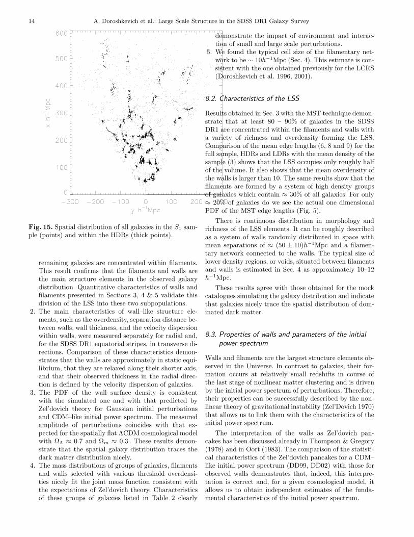
The spatial galaxy distribution for the S1 samples isplotted in Fig. 15; galaxies in HDRs are highlighted.

8.1. Main results

The main results of our investigation can be summarizedas follows:

1. The analysis performed in Sec. 3 with the MST tech-nique confirms that about half of galaxies are situatedwithin rich wall–like structures and the majority of the


Fig. 15. Spatial distribution of all galaxies in the S1 sam-ple (points) and within the HDRs (thick points).

remaining galaxies are concentrated within filaments.This result confirms that the filaments and walls arethe main structure elements in the observed galaxydistribution. Quantitative characteristics of walls andfilaments presented in Sections 3, 4 & 5 validate thisdivision of the LSS into these two subpopulations.

2. The main characteristics of wall–like structure ele-ments, such as the overdensity, separation distance be-tween walls, wall thickness, and the velocity dispersionwithin walls, were measured separately for radial and,for the SDSS DR1 equatorial stripes, in transverse di-rections. Comparison of these characteristics demon-strates that the walls are approximately in static equi-librium, that they are relaxed along their shorter axis,and that their observed thickness in the radial direc-tion is defined by the velocity dispersion of galaxies.

3. The PDF of the wall surface density is consistentwith the simulated one and with that predicted byZel’dovich theory for Gaussian initial perturbationsand CDM–like initial power spectrum. The measuredamplitude of perturbations coincides with that ex-pected for the spatially flat ΛCDM cosmological modelwith ΩΛ ≈ 0.7 and Ωm ≈ 0.3 . These results demon-strate that the spatial galaxy distribution traces thedark matter distribution nicely.

4. The mass distributions of groups of galaxies, filamentsand walls selected with various threshold overdensi-ties nicely fit the joint mass function consistent withthe expectations of Zel’dovich theory. Characteristicsof these groups of galaxies listed in Table 2 clearly

demonstrate the impact of environment and interac-tion of small and large scale perturbations.

5. We found the typical cell size of the filamentary net-work to be ∼ 10h−1Mpc (Sec. 4). This estimate is con-sistent with the one obtained previously for the LCRS(Doroshkevich et al. 1996, 2001).

8.2. Characteristics of the LSS

Results obtained in Sec. 3 with the MST technique demon-strate that at least 80 – 90% of galaxies in the SDSSDR1 are concentrated within the filaments and walls witha variety of richness and overdensity forming the LSS.Comparison of the mean edge lengths (6, 8 and 9) for thefull sample, HDRs and LDRs with the mean density of thesample (3) shows that the LSS occupies only roughly halfof the volume. It also shows that the mean overdensity ofthe walls is larger than 10. The same results show that thefilaments are formed by a system of high density groupsof galaxies which contain ≈ 30% of all galaxies. For only≈ 20% of galaxies do we see the actual one dimensionalPDF of the MST edge lengths (Fig. 5).

There is continuous distribution in morphology andrichness of the LSS elements. It can be roughly describedas a system of walls randomly distributed in space withmean separations of ≈ (50 ± 10)h−1Mpc and a filamen-tary network connected to the walls. The typical size oflower density regions, or voids, situated between filamentsand walls is estimated in Sec. 4 as approximately 10–12h−1Mpc.

These results agree with those obtained for the mockcatalogues simulating the galaxy distribution and indicatethat galaxies nicely trace the spatial distribution of dom-inated dark matter.

8.3. Properties of walls and parameters of the initial

power spectrum

Walls and filaments are the largest structure elements ob-served in the Universe. In contrast to galaxies, their for-mation occurs at relatively small redshifts in course ofthe last stage of nonlinear matter clustering and is drivenby the initial power spectrum of perturbations. Therefore,their properties can be successfully described by the non-linear theory of gravitational instability (Zel’Dovich 1970)that allows us to link them with the characteristics of theinitial power spectrum.

The interpretation of the walls as Zel’dovich pan-cakes has been discussed already in Thompson & Gregory(1978) and in Oort (1983). The comparison of the statisti-cal characteristics of the Zel’dovich pancakes for a CDM–like initial power spectrum (DD99, DD02) with those forobserved walls demonstrates that, indeed, this interpre-tation is correct and, for a given cosmological model, itallows us to obtain independent estimates of the funda-mental characteristics of the initial power spectrum.


The estimates of the mean wall surface density, 〈qw〉,and the amplitude of initial perturbations, 〈τm〉, listed inTable 1 are consistent with each other and with thosefound for the LCRS and DURS. They are also close tothose found for the simulated DM distribution and forthe mock galaxy catalogs (Cole et al. 1998) prepared fora spatially flat ΛCDM cosmological model with ΩΛ = 0.7,Ωm = 0.3 and σ8 = 1.05. As was shown in Sec. 5.3 (20),(21) and (22), the PDFs of both observed and simulatedwall surface density plotted in Figs. 10 and 11 coincidewith those theoretically expected (15) for Gaussian initialperturbations with a CDM–like power spectrum (DD99;DD02).

Averaging of both 〈qw〉 and 〈τm〉 listed in Table 1 al-lows us to estimate the mean values as follows:

〈qw〉 = (0.38 ± 0.06)(Γ/0.2) , (29)

τm = (0.24 ± 0.02)√

Γ/0.2 . (30)

These values are consistent with the best estimates of thesame amplitude (Spergel et al. 2003) for the ΛCDM cos-mological model with Γ = 0.2

σ8 ≈ 0.9 ± 0.1, τ ≈ 0.22 ± 0.02 , (31)

These results verify that galaxies nicely trace the LSSformed mainly by the dark matter distribution and theobserved walls are recently formed Zel’dovich pancakes.They also verify the Gaussian distribution of initial per-turbations and coincide with the Harrison – Zel’dovichprimordial power spectrum.

Comparison of other wall characteristics measured inradial and transverse directions indicate that the wallsare gravitationally confined and relaxed along the shorteraxis. The same comparison allows us to find the true walloverdensity, wall thickness, and the radial velocity disper-sion of galaxies within walls. As is seen from relation (18),these values are quite self–consistent.

8.4. Mass function of structure elements

The samples of walls, filaments, and groups of galaxies inthe SDSS DR1 selected using different threshold overden-sities allow us to measure their mass functions, to tracetheir dependence on the threshold overdensity and envi-ronment, and to compare them with the expectations ofZel’dovich theory.

This comparison verifies that for lower threshold over-densities for both filaments and wall–like structure ele-ments, the shape of the observed mass functions is consis-tent with the expectations of Zel’dovich theory. However,for high density groups of galaxies some deficit of low massgroups caused, in particular, by selection effects and en-hanced by the restrictions inherent in our procedure forgroup-finding leads to a stronger difference between theobserved and expected mass functions for Msel ≤ 〈Msel〉.The same factors distort the observed mass functions forgroups selected within LDRs.

Let us note that mass functions (26, 27, & 28) areclosely linked with the initial power spectrum. This ismanifested as a suppression of the PDFs at Msel ≤ 〈Msel〉and is proportional to exp[−(M/〈Msel〉)1/3] at Msel ≥〈Msel〉. They differ from the mass function of galaxy clus-ters and the probable mass function of observed galaxieswhich are formed on account of multi–step merging of lessmassive clouds and are described by a power law with anegative power index at Msel ≤ 〈Msel〉 and an exponen-tial cutoff ∝ exp[−(M/〈Msel〉) at Msel ≥ 〈Msel〉 (see e.g.Silk & White 1978).

8.5. Interaction of large and small scale perturbations

The data listed in Table 2 shows that the majority ofhigh density groups of galaxies and the main fraction ofgalaxies related to these groups (up to 80 – 90%) are sit-uated within HDRs. These results illustrate the influenceof environment on galaxy formation and the clusteringof luminous matter. It also indicates the importance ofinteractions of small and large scale perturbations for theformation of the observed LSS. This problem was also dis-cussed in Einasto et al. (2003a,b).

These differences are partly enhanced by the influenceof selection effects. Indeed, the majority of HDRs are situ-ated at moderate distances D ∼ 150 − 300h−1Mpc wherethis influence is not so strong. On the other hand the LDRsalso include all galaxies situated in the farthest low den-sity regions. However, as was shown in DD02 significantdifferences between the characteristics of clouds separatedwithin HDRs and LDRs is seen even for simulated clus-tering of dark matter.

These results are consistent with the high concentra-tion of observed galaxies within the filaments and wallsforming the LSS noted in Sec. 8.2. Bearing in mind thatthe mean density of luminous matter does not exceed 10%of the full matter density of the Universe we can con-clude that galaxies are formed at high redshifts presum-ably within compressed regions which are now seen as el-ements of LSS.

A natural explanation for both of these differences andthe high concentration of galaxies within the LSS elementsis the interaction of small and large scale perturbationswhen large scale compression of matter accelerates theformation of small scale high density clouds. Such interac-tions may also explain the existence of large voids similarto the Bootes void where formation of galaxies has beenstrongly suppressed.

8.6. Possible rich clusters of galaxies

The MST technique generalizes the standard ‘friends–of–friends’ method of the selection of denser clouds and ofprobable clusters of galaxies. However, first attempts ofsuch selection presented in Sec. 6 show that there is an es-sential difference between the selected high density cloudsand x-ray sources. The nature of this difference is not yet


clear and perhaps it will be eliminated after the intro-duction of stronger criteria for the selection of probableclusters of galaxies from the survey.

8.7. Final comments

The SDSS (York et al. 2000; Stoughton et al. 2002;Abazajian et al. 2003) and 2dF (Colless et al. 2001)galaxy redshift surveys provide deep and broad vistas withwhich cosmologists may study the galaxy distribution onextremely large scales –scales on which the imprint fromthe primordial fluctuation spectrum has not been erased.

In this paper, we have used the SDSS DR1 to investi-gate the galaxy distribution at such large scales. We haveconfirmed our earlier results, based on the LCRS andDURS samples, that galaxies are distributed in roughlyequal numbers between two different environments: fil-aments, which dominate low density regions, and walls,which dominate high density regions. Although differentin character, these two environments together form a frag-mented joint random network of galaxies – the cosmic web.

Comparison with theory strongly supports the ideathat the properties of the observed walls are consis-tent with those for Zel’dovich pancakes formed froma Gaussian spectrum of initial perturbations for a flatΛCDM Universe (ΩΛ ≈ 0.7, Ωm ≈ 0.3). These results areconsistent with the estimate of Γ = 0.20±0.03 obtained inPercival et al. (2001) for the 2dF Galaxy Redshift Survey(see also Spergel et al. 2003).

Such analysis one allows to obtain some important ba-sic conclusions regarding the properties and the process offormation and evolution of the large scale structure of theUniverse. With future public releases of the SDSS dataset, we hope to refine these conclusions.

Acknowledgments

We thank Shiyin Shen of the Max-Planck-Institut furAstrophysik and Jorg Retzlaff of the Max-Planck-Institutfur Extraterrestrial Physics for useful discussions regard-ing this work.

Funding for the creation and distribution of theSDSS Archive has been provided by the Alfred P. SloanFoundation, the Participating Institutions, the NationalAeronautics and Space Administration, the NationalScience Foundation, the US Department of Energy, theJapanese Monbukagakusho, and the Max Planck Society.The SDSS Web site is http://www.sdss.org/.The Participating Institutions are the University ofChicago, Fermilab, the Institute for Advanced Study, theJapan Participation Group, the Johns Hopkins University,the Max Planck Institute for Astronomy (MPIA), the MaxPlanck Institute for Astrophysics (MPA), New MexicoState University, Princeton University, the United StatesNaval Observatory, and the University of Washington.This paper was supported in part by Denmark’sGrundforskningsfond through its support for an establish-ment of the Theoretical Astrophysics Center.

References

Abazajian, K., Adelman–McCarthy, J. K., Agueros,M. A., Allam, S. S., & the SDSS Collaboration. 2003,ArXiv Astrophysics e-prints, 5492

Bohringer, H., Voges, W., Huchra, J. P., McLean, B.,Giacconi, R., Rosati, P., Burg, R., Mader, J., Schuecker,P., Simic, D., Komossa, S., Reiprich, T. H., Retzlaff, J.,& Trumper, J. 2000, ApJS, 129, 435

Barrow, J. D., Bhavsar, S. P., & Sonoda, D. H. 1985,MNRAS, 216, 17

Baugh, C. M. & Efstathiou, G. 1993, MNRAS, 265, 145Bhavsar, S. P. & Ling, E. N. 1988, ApJ, 331, L63Buryak, O. & Doroshkevich, A. 1996, A&A, 306, 1Cole, S., Hatton, S., Weinberg, D. H., & Frenk, C. S. 1998,

MNRAS, 300, 945Colless, M., Dalton, G., Maddox, S., Sutherland, W.,

Norberg, P., Cole, S., Bland-Hawthorn, J., Bridges, T.,Cannon, R., Collins, C., Couch, W., Cross, N., Deeley,K., De Propris, R., Driver, S. P., Efstathiou, G., Ellis,R. S., Frenk, C. S., Glazebrook, K., Jackson, C., Lahav,O., Lewis, I., Lumsden, S., Madgwick, D., Peacock,J. A., Peterson, B. A., Price, I., Seaborne, M., & Taylor,K. 2001, MNRAS, 328, 1039

Demianski, M. & Doroshkevich, A. G. 1999, MNRAS, 306,779

—. 2002, ArXiv Astrophysics e-prints, 6282Demianski, M., Doroshkevich, A. G., & Turchaninov, V.

2000, MNRAS, 318, 1189—. 2003, MNRAS, 340, 525Doroshkevich, A. G., Fong, R., McCracken, H. J.,

Ratcliffe, A., Shanks, T., & Turchaninov, V. I. 2000,MNRAS, 315, 767

Doroshkevich, A. G., Tucker, D. L., Fong, R.,Turchaninov, V., & Lin, H. 2001, MNRAS, 322,369

Doroshkevich, A. G., Tucker, D. L., Oemler, A. J.,Kirshner, R. P., Lin, H., Shectman, S. A., Landy, S. D.,& Fong, R. 1996, MNRAS, 283, 1281

Einasto, M., Einasto, J., Muller, V., Heinamaki, P., &Tucker, D. L., 2003, A&A, 401, 851

Einasto, J., Hutsi, G., Einasto, M., Saar, E., Tucker, D. L.,Muller, V., Heinamaki, P., & Allam, S. S. 2003, A&A,405, 425

Fukugita, M., Ichikawa, T., Gunn, J. E., Doi, M.,Shimasaku, K., & Schneider, D. P. 1996, AJ, 111, 1748

Gunn, J. E., Carr, M., Rockosi, C., Sekiguchi, M., & theSDSS Collaboration. 1998, AJ, 116, 3040

Huchra, J. P. & Geller, M. J. 1982, ApJ, 257, 423Jenkins, A., Frenk, C. S., Pearce, F. R., Thomas, P. A.,

Colberg, J. M., White, S. D. M., Couchman, H. M. P.,Peacock, J. A., Efstathiou, G., & Nelson, A. H. 1998,ApJ, 499, 20

Kruskal, J. B. 1956, Proc. Amer. Math. Soc., 7, 48Oort, J. H. 1983, ARA&A, 21, 373Percival, W. J., Baugh, C. M., Bland-Hawthorn, J.,

Bridges, T., Cannon, R., Cole, S., Colless, M., Collins,C., Couch, W., Dalton, G., De Propris, R., Driver, S. P.,

http://www.sdss.org/


Efstathiou, G., Ellis, R. S., Frenk, C. S., Glazebrook, K.,Jackson, C., Lahav, O., Lewis, I., Lumsden, S., Maddox,S., Moody, S., Norberg, P., Peacock, J. A., Peterson,B. A., Sutherland, W., & Taylor, K. 2001, MNRAS,327, 1297

Prim. 1957, Bell System Tech. J., 36, 1389Ratcliffe, A., Shanks, T., Broadbent, A., Parker, Q. A.,

Watson, F. G., Oates, A. P., Fong, R., & Collins, C. A.1996, MNRAS, 281, L47+

Schmalzing, J., Gottlober, S., Klypin, A. A., & Kravtsov,A. V. 1999, MNRAS, 309, 1007

Shandarin, S. F. & Zeldovich, Y. B. 1989, Reviews ofModern Physics, 61, 185

Shectman, S. A., Landy, S. D., Oemler, A., Tucker, D. L.,Lin, H., Kirshner, R. P., & Schechter, P. L. 1996, ApJ,470, 172

Sheth, J. V., Sahni, V., Shandarin, S. F., &Sathyaprakash, B. S. 2002, ArXiv Astrophysicse-prints, 10136

Silk, J. & White, S. D. 1978, ApJl, 223, L59Spergel, D. N., Verde, L., Peiris, H. V., Komatsu, E.,

Nolta, M. R., Bennett, C. L., Halpern, M., Hinshaw,G., Jarosik, N., Kogut, A., Limon, M., Meyer, S. S.,Page, L., Tucker, G. S., Weiland, J. L., Wollack, E., &Wright, E. L. 2003, ArXiv Astrophysics e-prints, 2209

Stoughton, C., Lupton, R. H., Bernardi, M., Blanton,M. R., & the SDSS Collaboration. 2002, AJ, 123, 485

Thompson, L. A. & Gregory, S. A. 1978, ApJ, 220, 809Tucker, D. L., Oemler, A. J., Hashimoto, Y., Shectman,

S. A., Kirshner, R. P., Lin, H., Landy, S. D., Schechter,P. L., & Allam, S. S. 2000, ApJS, 130, 237

van de Weygaert, M. A. M. 1991, Ph.D Thesis (Leiden:Rijksuniversiteit, —c1991)

York, D. G., Adelman, J., Anderson, J. E., Anderson,S. F., & the SDSS Collaboration. 2000, AJ, 120, 1579

Zel’Dovich, Y. B. 1970, A&A, 5, 84

Documents

Large Scale Structure in the SDSS DR1 Galaxy Surveylss.fnal.gov/archive/2003/pub/fermilab-pub-03-253-a.pdf · A. Doroshkevich et al.: Large Scale Structure in the SDSS DR1 Galaxy